ch 3: discrete rv - github pages
TRANSCRIPT
Summer 2017 UAkron Dept. of Stats [3470 : 461/561] Applied Statistics
Ch 3: Discrete RV
Contents1 PMF and CDF 2
1.1 Random Variable . . . . . . . . . . . . . . . . . . . . . . . . . . . . . . . . . . . . . . . . . . . . . . . . . . . . . . . . . . . . . . . . 3
1.2 PMF and CDF . . . . . . . . . . . . . . . . . . . . . . . . . . . . . . . . . . . . . . . . . . . . . . . . . . . . . . . . . . . . . . . . . 4
2 Expected Value and Variance 14
2.1 The Expected value (Theoretical Mean) . . . . . . . . . . . . . . . . . . . . . . . . . . . . . . . . . . . . . . . . . . . . . . . . . . . 15
2.2 Expectation is a long-run average . . . . . . . . . . . . . . . . . . . . . . . . . . . . . . . . . . . . . . . . . . . . . . . . . . . . . . . 17
2.3 How to calculate E(g(X)) . . . . . . . . . . . . . . . . . . . . . . . . . . . . . . . . . . . . . . . . . . . . . . . . . . . . . . . . . . . 21
2.4 (Theoretical) Variance . . . . . . . . . . . . . . . . . . . . . . . . . . . . . . . . . . . . . . . . . . . . . . . . . . . . . . . . . . . . . 23
3 Popular Discrete Distributions 27
3.1 Binomial Random Variable . . . . . . . . . . . . . . . . . . . . . . . . . . . . . . . . . . . . . . . . . . . . . . . . . . . . . . . . . . 29
3.2 Negative Binomial Random Variable . . . . . . . . . . . . . . . . . . . . . . . . . . . . . . . . . . . . . . . . . . . . . . . . . . . . . 41
3.3 Hypergeometric Random Variable . . . . . . . . . . . . . . . . . . . . . . . . . . . . . . . . . . . . . . . . . . . . . . . . . . . . . . 46
3.4 Poisson Random Variable . . . . . . . . . . . . . . . . . . . . . . . . . . . . . . . . . . . . . . . . . . . . . . . . . . . . . . . . . . . 56
3.5 R code for the Four Distributions . . . . . . . . . . . . . . . . . . . . . . . . . . . . . . . . . . . . . . . . . . . . . . . . . . . . . . . 65
June 19, 2017

1
. PMF and CDF
[ToC]
2

1.1 Random Variable
[ToC]
is a function whose domain is a sample space, and whose range is a real numbers.
Discrete Random Variable is a r.v. whose range is a finite or countably infinite set.
Continuous Variable is a r.v. whose range is a interval on a real line or a disjoint union of such
intervals. It also must satisfy that for any constant c, P (X = c) = 0.
Example
1. Throw a die: {1} → 1
2. Throw two dice at once and add: {2, 5} → 7
3

1.2 PMF and CDF
[ToC]
• Probability Mass Function: (pmf) of a discrete RV is defined as
p(x) = P (X = x)
• Cumulative Distribution Function: (cdf) of a discrete random variable X is defined as
F (x) = P (X ≤ x)
4
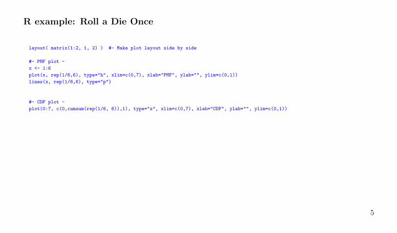
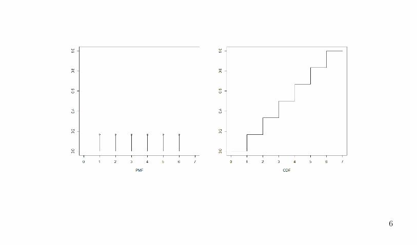
R example: Roll a Die Once
layout( matrix(1:2, 1, 2) ) #- Make plot layout side by side
#- PMF plot -
x <- 1:6
plot(x, rep(1/6,6), type="h", xlim=c(0,7), xlab="PMF", ylab="", ylim=c(0,1))
lines(x, rep(1/6,6), type="p")
#- CDF plot -
plot(0:7, c(0,cumsum(rep(1/6, 6)),1), type="s", xlim=c(0,7), xlab="CDF", ylab="", ylim=c(0,1))
5
6

R example: Roll a Die Twice
layout( matrix(1:2, 1, 2) ) #- Make plot layout side by side
#- PMF plot -
x <- 2:12
pmf1 <- c(1,2,3,4,5,6,5,4,3,2,1)/36
plot(x, pmf1, type="h", xlim=c(1,13), xlab="PMF", ylab="", ylim=c(0,1))
lines(x, pmf1, type="p")
#- CDF plot -
plot(c(1,x,13), c(0,cumsum(pmf1),1), type="s", xlim=c(1,13), xlab="CDF", ylab="", ylim=c(0,1))
7

8
PMF and CDF
• You can calculate CDF from PMF, or vice varsa.
• CDF always start at 0, and end at 1.
• pmf at any point must be ≥ 0.
• If you add all values of pmf, it must add up to 1.
9
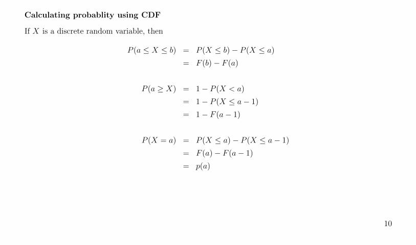
Calculating probablity using CDF
If X is a discrete random variable, then
P (a ≤ X ≤ b) = P (X ≤ b)− P (X ≤ a)
= F (b)− F (a)
P (a ≥ X) = 1− P (X < a)
= 1− P (X ≤ a− 1)
= 1− F (a− 1)
P (X = a) = P (X ≤ a)− P (X ≤ a− 1)
= F (a)− F (a− 1)
= p(a)
10
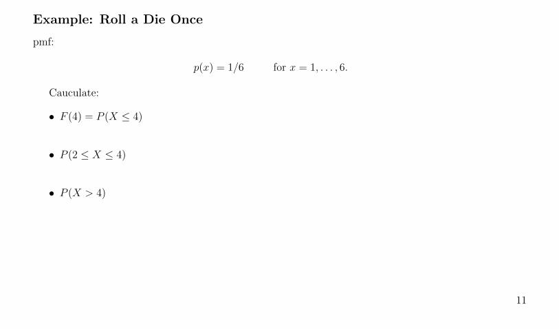
Example: Roll a Die Once
pmf:
p(x) = 1/6 for x = 1, . . . , 6.
Cauculate:
• F (4) = P (X ≤ 4)
• P (2 ≤ X ≤ 4)
• P (X > 4)
11

Exercises:
Given the CDF:
F (1) = .2, F (2) = .35, F (3) = .60, F (4) = .90, F (5) = .95, F (6) = 1
Calculate the following:
P (X > 3)
.
P (2 ≤ X ≤ 5)
.
P (2 < X < 5)
.
p(2)
12
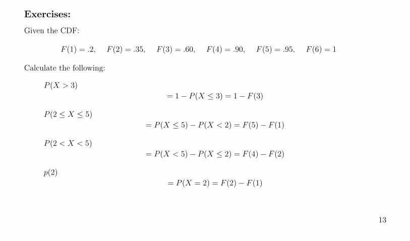
Exercises:
Given the CDF:
F (1) = .2, F (2) = .35, F (3) = .60, F (4) = .90, F (5) = .95, F (6) = 1
Calculate the following:
P (X > 3)
= 1− P (X ≤ 3) = 1− F (3)
P (2 ≤ X ≤ 5)
= P (X ≤ 5)− P (X < 2) = F (5)− F (1)
P (2 < X < 5)
= P (X < 5)− P (X ≤ 2) = F (4)− F (2)
p(2)
= P (X = 2) = F (2)− F (1)
13
2
. Expected Value and Variance
[ToC]
14

2.1 The Expected value (Theoretical Mean)
[ToC]
• Expected Value of a random variable X, whose range is x1, x2, x3, . . . xn is defined as
E(X) = µ =n∑i=1
xi · p(xi)
15

Example: Throw a Die Once
Suppose you are given pmf:
# 1 2 3 4 5 6
p(x) 16
16
16
16
16
16
Then the expectation is
E(X) = 1 · 1
6+ 2 · 1
6+ 3 · 1
6+ 4 · 1
6+ 5 · 1
6+ 6 · 1
6= 3.5
16

2.2 Expectation is a long-run average
[ToC]
Theoretical Mean (Expectation)
E(X) = 1 ·(1
6
)+ 2 ·
(1
6
)+ 3 ·
(1
6
)+ 4 ·
(1
6
)+ 5 ·
(1
6
)+ 6 ·
(1
6
)= 3.5
Sample Mean (Average)
X̄ = 1 ·(
Rel. Freq. of #1)
+ 2 ·(
Rel. Freq. of #2)
+ 3 ·(
Rel. Freq. of #3)
+ 4 ·(
Rel. Freq. of #4)
+ 5 ·(
Rel. Freq. of #5)
+ 6 ·(
Rel. Freq. of #6)
= ...
• Sample Mean converges to The Expectation as n→∞.
17
Example: Pooled Blood Testing
• Each blood sample has .1 change of testing positive.
• New procedure called ”pooled testing” combines 10 blood sample before testing.
• If comes back negative, no further test is done. If comes back positive, then 10 more test must be
done using individual samples.
• What is the long-run average of the test number in the new scheme?
18

Example: Casino Simplified
• You charge each person $1 to play this game.
• Each player has 1% chance of winning $100.
• Does this make sence as business?
• What if you change 1% chance to .5% chance?
19
Example: Casino Simplified
• You charge each person $1 to play this game.
• Each player has 1% chance of winning $100.
• Does this make sence as business?
• What if you change 1% chance to .5% chance?
1(.99) + (−99)(.01) = 0
1(.995) + (−99)(.005) = .5
20
2.3 How to calculate E(g(X))
• Expected Value of a function of random variable X, say g(X) is defined as
E(g(X)
)=
n∑i=1
g(xi) · p(xi)
• If a and b are constants, then
E(aX + b) = aE(X) + b
21

Example: Throw a Die Once
Recall Let a random variable X to be a number of the rolled die. Then
E(X2) = 12 · 1
6+ 22 · 1
6+ 32 · 1
6+ 42 · 1
6+ 52 · 1
6+ 62 · 1
6= 15.16667
Note that they are not equal to(E(X)
)2.
E(3X + 5) = (3 · 1 + 5) · 1
6+ (3 · 2 + 5) · 1
6+ (3 · 3 + 5) · 1
6
+(3 · 4 + 5) · 1
6+ (3 · 5 + 5) · 1
6+ (3 · 6 + 5) · 1
6= 15.5
Note that it is equal to 3E(X) + 5.
22
2.4 (Theoretical) Variance
[ToC]
• Variance of a random variable X is defined as
V (X) = σ2 =n∑i=1
(xi − µ)2 · p(xi) = E[(X − µ
)2]. = E(X2)−
(E(X)
)2Note that µ = E(X). Standard Deviation of X is defined as σ =
√σ2.
• Compare to Sample Variance
S2 =1
n− 1
n∑i=1
(Xi − X̄)2
23
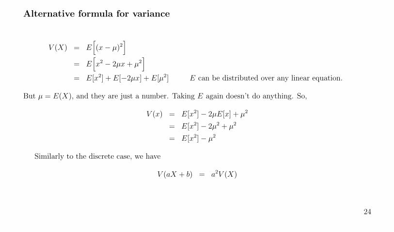
Alternative formula for variance
V (X) = E[(x− µ)2
]= E
[x2 − 2µx+ µ2
]= E[x2] + E[−2µx] + E[µ2] E can be distributed over any linear equation.
But µ = E(X), and they are just a number. Taking E again doesn’t do anything. So,
V (x) = E[x2]− 2µE[x] + µ2
= E[x2]− 2µ2 + µ2
= E[x2]− µ2
Similarly to the discrete case, we have
V (aX + b) = a2V (X)
24

Example: Throw a Die Once
Suppose you are given pmf:
# 1 2 3 4 5 6
p(x) 16
16
16
16
16
16
• Expectation was E(X) = 3.5.
• Now calcualte E(X2),
E(X2) = 12 · 1
6+ 22 · 1
6+ 32 · 1
6+ 42 · 1
6+ 52 · 1
6+ 62 · 1
6= 15.167
• So the variance is
V (X) = E(X2)− [E(X)]2 = 15.167− 3.52 = 2.917.
25
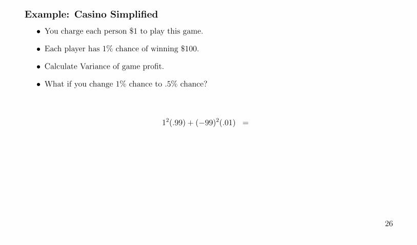
Example: Casino Simplified
• You charge each person $1 to play this game.
• Each player has 1% chance of winning $100.
• Calculate Variance of game profit.
• What if you change 1% chance to .5% chance?
12(.99) + (−99)2(.01) =
26
3
. Popular Discrete Distributions
[ToC]
27
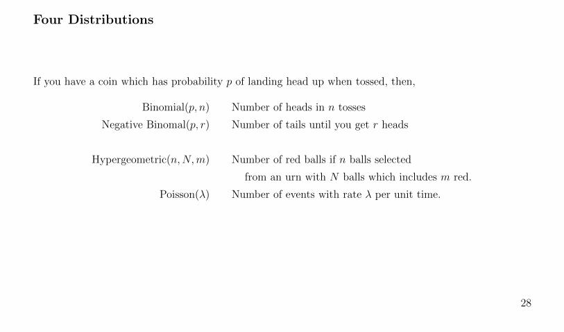
Four Distributions
If you have a coin which has probability p of landing head up when tossed, then,
Binomial(p, n) Number of heads in n tosses
Negative Binomal(p, r) Number of tails until you get r heads
Hypergeometric(n,N,m) Number of red balls if n balls selected
from an urn with N balls which includes m red.
Poisson(λ) Number of events with rate λ per unit time.
28
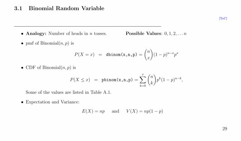
3.1 Binomial Random Variable
[ToC]
• Analogy: Number of heads in n tosses. Possible Values: 0, 1, 2, . . . n
• pmf of Binomial(n, p) is
P (X = x) = dbinom(x,n,p) =
(n
x
)(1− p)n−xpx
• CDF of Binomial(n, p) is
P (X ≤ x) = pbinom(x,n,p) =x∑k=0
(n
k
)pk(1− p)n−k,
Some of the values are listed in Table A.1.
• Expectation and Variance:
E(X) = np and V (X) = np(1− p)
29

Derivation of Binomial pmf
30

R code for Binomial(n, p)
x =[number of heads] n =[number of flip] p =[prob. of head in 1 flip]
pbinom(3,10,.5) #- F(3): CDF of Bin(n=10, p=.5) at x=3
dbinom(3,10,.5) #- p(3): pmf of Bin(n=10, p=.5) at x=3
layout( matrix(1:2, 1, 2) ) #- Make plot layout side by side
x <- 0:11
plot(x, dbinom(x, 10, .5), type="h", ylim=c(0,1)) #- PMF plot -
plot(x, pbinom(x, 10, .5), type="s", ylim=c(0,1)) #- CDF plot -
31

32
Example: Crystal Picking
A company that produces fine crystal knows from experience that 10% of its goblets have cosmetic flaws
and must be classified as “seconds”.
1. Among six randomly selected goblets, how likely is it that only one is a second?
2. Among six randomly selected goblets, what is the probability that at least two are seconds?
33
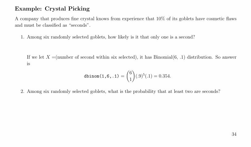
Example: Crystal Picking
A company that produces fine crystal knows from experience that 10% of its goblets have cosmetic flaws
and must be classified as “seconds”.
1. Among six randomly selected goblets, how likely is it that only one is a second?
If we let X =(number of second within six selected), it has Binomial(6, .1) distribution. So answer
is
dbinom(1,6,.1) =
(6
1
)(.9)5(.1) = 0.354.
2. Among six randomly selected goblets, what is the probability that at least two are seconds?
34
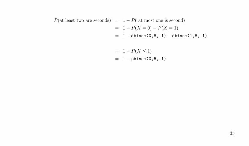
P (at least two are seconds) = 1− P ( at most one is second)
= 1− P (X = 0)− P (X = 1)
= 1− dbinom(0,6,.1)− dbinom(1,6,.1)
= 1− P (X ≤ 1)
= 1− pbinom(0,6,.1)
35
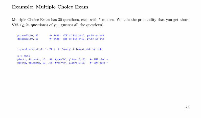
Example: Multiple Choice Exam
Multiple Choice Exam has 30 questions, each with 5 choices. What is the probability that you get above
80% (≥ 24 questions) of you guesses all the questions?
pbinom(3,10,.5) #- F(3): CDF of Bin(n=10, p=.5) at x=3
dbinom(3,10,.5) #- p(3): pmf of Bin(n=10, p=.5) at x=3
layout( matrix(1:2, 1, 2) ) #- Make plot layout side by side
x <- 0:11
plot(x, dbinom(x, 10, .5), type="h", ylim=c(0,1)) #- PMF plot -
plot(x, pbinom(x, 10, .5), type="s", ylim=c(0,1)) #- CDF plot -
36
Example: Psychic or not
One person claims to have a phychic power. He claims that when one card is chosen out of 4 cards having
different symbols, (star, triangle, circle, cross), he can tell the symbol while the chosen card is inside an
envelope.
If he is allowed to try 10 times, over what % of correct answer is impressive?
37
Example: Minority Represented in a Commitiee
Suppose among large number of students. 20% of them are minority. To form a student council, 10 students
are randomly selected. What is the probability that the minority is over-represented or under-represented?
38

Example: Best of 7
39
Example: Catch a cheater?
Suppose you flip a coin n times. When a coin is not fair, and P (Head), how many times do you have to
filp to see the difference in behavior?
40

3.2 Negative Binomial Random Variable
[ToC]
• Analogy: Number of tails until you get r th head. Possible Values: 0, 1, 2, 3,. . .
• pmf of NBin(r, p)
P (X = x) = dnbinom(x, r, p) =
(x+ r − 1
r − 1
)(1− p)xpr for x = 0, 1, 2, . . .
=
(x+ r − 1
x
)(1− p)xpr for x = 0, 1, 2, . . .
• CDF of NBin(r, p)
P (X ≤ x) = pnbinom(x, r, p)
• Expectation and Variance
E(X) =r(1− p)
pand V (X) =
r(1− p)p2
41
Derivation of Negative Binomial pmf
42

R code for Negative Binomial(r, p)
x =[number of tails before r th head]
r =[number of heads to flip to]
p =[prob. of head in 1 flip]
pnbinom(3,5,.3) #- F(3): CDF of NegBin(n=5, p=.4) at x=3
dnbinom(3,5,.3) #- p(3): pmf of NegBin(n=5, p=.4) at x=3
layout( matrix(1:2, 1, 2) ) #- Make plot layout side by side
x <- 0:30
plot(x, dnbinom(x, 5, .3), type="h", ylim=c(0,.5)) #- PMF plot -
plot(x, pnbinom(x, 5, .3), type="s", ylim=c(0,1)) #- CDF plot -
43

Figure 1: r=5, p=.3
44

Example: Shoot free throw until you make 10 shots
Suppose your free-throw percentage is 90%. Assume independence between each shots. You can’t go home
until you make 10 baskets, how many shots do you need to take before you go home?
45

3.3 Hypergeometric Random Variable
[ToC]
• Analogy: There are N balls whith m reds. Pick n balls at once. X =[# of red picked].
• Pmf of Hypergeometric(n,m,N) is
P (X = x) = dhyper(x, n, N-m, n) =
(mx
)(N−mn−x
)(Nn
)for max(0, n−N +m) ≤ x ≤ min(n,m), and 0 otherwise.
• Expectation and Mean
E(X) =nm
Nand V (X) =
N − nN − 1
nm
N
(1− m
N
)
46

Derivation of Hypergeometric pmf
47

R code for Hypergeometric(n,m,N)
x =[number of heads]
n =[number of balls picked]
m =[number of Red balls]
N =[number of total balls]
dhyper(3,4,6,5) #- p(3): pmf of Hypergeoretric(m=4, N-m=6 ,n=5) at x=3 (That means N=10)
phyper(3,4,6,5) #- F(3): CDF of Hypergeoretric(m=4, N-m=6 ,n=5) at x=3
layout( matrix(1:2, 1, 2) ) #- Make plot layout side by side
x <- 0:10
plot(x, dhyper(x, 4,6,5), type="h", ylim=c(0,1)) #- PMF plot -
plot(x, phyper(x, 4,6,5), type="s", ylim=c(0,1)) #- CDF plot -
48
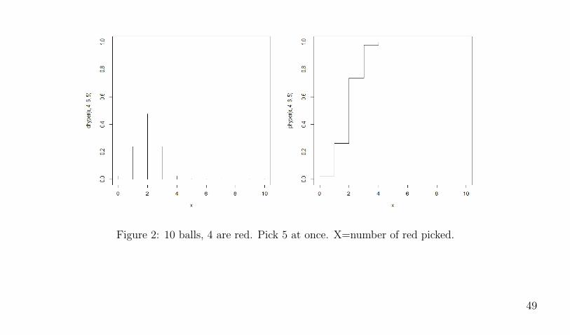
Figure 2: 10 balls, 4 are red. Pick 5 at once. X=number of red picked.
49

Example: Rock sampling
A geologist has collected 10 specimens of basaltic rock and 10 specimens of granite. The geologist instructs
a laboratory assistant to randomly select 15 of the specimen for analysis.
a What is the pmf of the number of granite specimen selected for analysis.
b What is the probability hat all specimens of one of the two types of rock are selected for analysis.
c What is the probability that the number of granite specimens selected for analysis is within 1 standard
deviation of its mean value?
50
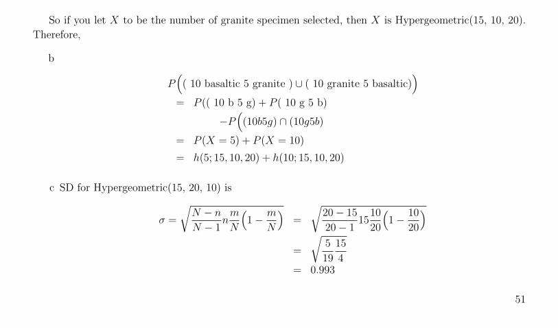
So if you let X to be the number of granite specimen selected, then X is Hypergeometric(15, 10, 20).
Therefore,
b
P(
( 10 basaltic 5 granite ) ∪ ( 10 granite 5 basaltic))
= P (( 10 b 5 g) + P ( 10 g 5 b)
−P(
(10b5g) ∩ (10g5b)
= P (X = 5) + P (X = 10)
= h(5; 15, 10, 20) + h(10; 15, 10, 20)
c SD for Hypergeometric(15, 20, 10) is
σ =
√N − nN − 1
nm
N
(1− m
N
)=
√20− 15
20− 115
10
20
(1− 10
20
)=
√5
19
15
4= 0.993
51
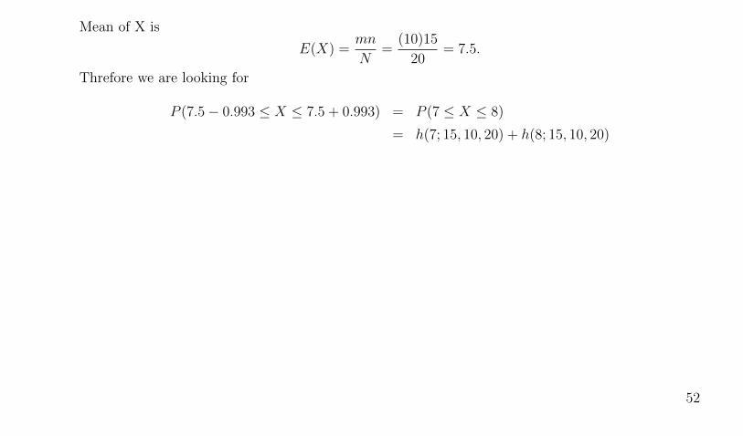
Mean of X is
E(X) =mn
N=
(10)15
20= 7.5.
Threfore we are looking for
P (7.5− 0.993 ≤ X ≤ 7.5 + 0.993) = P (7 ≤ X ≤ 8)
= h(7; 15, 10, 20) + h(8; 15, 10, 20)
52

Example: Capture-Recapture
One popular method of estimating population size of wild animal is called Capture-Recapture method.
First, you capture m subjects, tag and release them. Then sometime later, you come back and capture n
subjects. Within this n subjects, we count how many of them has a tag. Let X be the number of tagged
subjects. Our logic is that since
E(X) =nm
N,
It must be that
X ≈ E(X) =nm
N.
If we go with this logic, then our estimator for N will be N̂ = nm/X.
If we use this estmator in the case (N = 500, n = 100,m = 100), what will be the accuracy of this
estimator N̂?
53
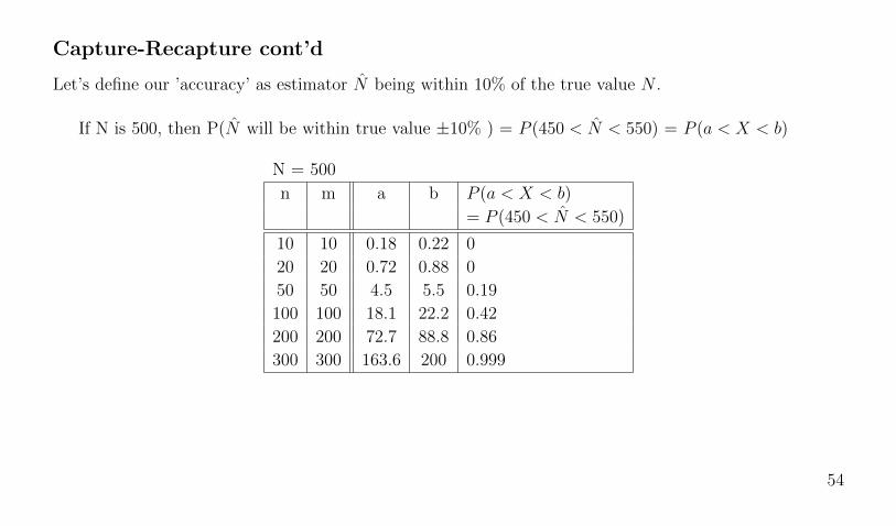
Capture-Recapture cont’d
Let’s define our ’accuracy’ as estimator N̂ being within 10% of the true value N .
If N is 500, then P(N̂ will be within true value ±10% ) = P (450 < N̂ < 550) = P (a < X < b)
N = 500
n m a b P (a < X < b)
= P (450 < N̂ < 550)
10 10 0.18 0.22 0
20 20 0.72 0.88 0
50 50 4.5 5.5 0.19
100 100 18.1 22.2 0.42
200 200 72.7 88.8 0.86
300 300 163.6 200 0.999
54
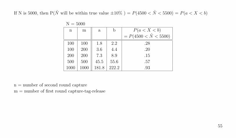
If N is 5000, then P(N̂ will be within true value ±10% ) = P (4500 < N̂ < 5500) = P (a < X < b)
N = 5000
n m a b P (a < X < b)
= P (4500 < N̂ < 5500)
100 100 1.8 2.2 .28
100 200 3.6 4.4 .20
200 200 7.3 8.9 .15
500 500 45.5 55.6 .57
1000 1000 181.8 222.2 .93
n = number of second round capture
m = number of first round capture-tag-release
55

3.4 Poisson Random Variable
[ToC]
• Analogy: events with rate λ per unit time. Possible Values: 0, 1, 2, 3, . . .
• pmf of Poisson(λ) is
P (X = x) = dpois(x, lambda) =e−λλx
x!
• Expectation and Variance:
E(X) = λ and V (X) = λ.
• Poisson as a limit If we let n→∞, p→ 0, in such a way that np→ λ, then the pmf
dbinom(x, n, p)→ dpois(x, lambda).
56

R code for Poisson(λ)
x =[number of events in a unit time] λ =[average number of events per unit time]
dpois(3,4) #- p(3): pmf of Poi(lambda=.5) at x=3
ppois(3,4) #- F(3): CDF of Poi(lambda=.5) at x=3
layout( matrix(1:2, 1, 2) ) #- Make plot layout side by side
x <- 0:12
plot(x, dpois(x, 4), type="h", ylim=c(0,1)) #- PMF plot -
plot(x, ppois(x, 4), type="s", ylim=c(0,1)) #- CDF plot -
57

58

When Time Units are Changed
59

Example: Number of Tornados
Suppose the number X of tornadoes observed in a particular region during a 1-year period has a Poisson
distribution with λ = 8.
1. What is the probability we get fewer than 4 tornados next year?
2. What is the probability we get fewer than 6 tornados in next two years?
60

Example: Number of Tornados
Suppose the number X of tornadoes observed in a particular region during a 1-year period has a Poisson
distribution with λ = 8.
1. What is the probability we get fewer than 4 tornados next year?
= P (X = 0) + P (X = 1) + P (X = 2) + P (X = 3)
= dpois(0,8) + dpois(1,8) + dpois(2,8) + dpois(3,8)
= P (X ≤ 3) = ppois(3, 8)
2. What is the probability we get fewer than 6 tornados in next two years?
For two-year period, number of tornados has Pois(16) distribution.
P (X ≤ 5) = ppois(5, 16)
�
61

Example: Aircraft arrivals
Suppose small aircraft arrive at a certain airport according to a Poisson process with rate α = 8 per hour,
so that the number of arrivals during a time period of t hours is a Poisson r.v. with λ = 8t.
1. What is the probability that exactly 6 small aircraft arrive during 1-hour period?
2. What are the expected value and standard deviation of the number of small aircraft that arrive
during a 90-min period?
3. What is the probability that at least 20 small aircraft arrive during 3 hour period?
62

Example: circuit boards
If proof testing of circuit boards, the probability that an particular diode will fail is .01. Suppose a circuit
board contains 200 diodes.
a How many diodes would you expect to fail, and what is the standard deviation of the number that
are expected to fail?
Here we have Binomial(200, .01), which can be approximated by Poisson(200 × .01). Therefore,
expected value is 2, and standard deviation is√
2.
b What is the approximate probability that at least four diodes will fail on a randomly selected board?
Since we are looking at Poisson(2),
P ( at least 4) = 1− P (X ≤ 3) = 1− .857 = .143
from the table A.2.
63
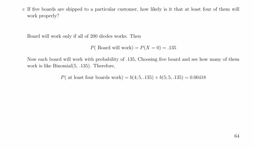
c If five boards are shipped to a particular customer, how likely is it that at least four of them will
work properly?
Board will work only if all of 200 diodes works. Then
P ( Board will work) = P (X = 0) = .135
Now each board will work with probability of .135, Choosing five board and see how many of them
work is like Binomial(5, .135). Therefore,
P ( at least four boards work) = b(4; 5, .135) + b(5; 5, .135) = 0.00418
64
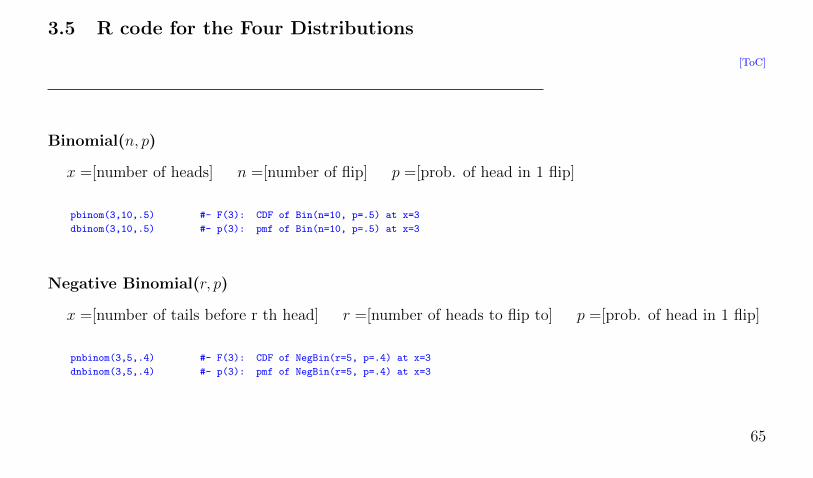
3.5 R code for the Four Distributions
[ToC]
Binomial(n, p)
x =[number of heads] n =[number of flip] p =[prob. of head in 1 flip]
pbinom(3,10,.5) #- F(3): CDF of Bin(n=10, p=.5) at x=3
dbinom(3,10,.5) #- p(3): pmf of Bin(n=10, p=.5) at x=3
Negative Binomial(r, p)
x =[number of tails before r th head] r =[number of heads to flip to] p =[prob. of head in 1 flip]
pnbinom(3,5,.4) #- F(3): CDF of NegBin(r=5, p=.4) at x=3
dnbinom(3,5,.4) #- p(3): pmf of NegBin(r=5, p=.4) at x=3
65

Hypergeometric(n,m,N)
x =[number of heads]
n =[number of balls picked]
m =[number of Red balls]
N =[number of total balls]
phyper(3,4,6,5) #- F(3): CDF of Hypergeoretric(m=4, N-m=6 ,n=5) at x=3 (That means N=10)
dhyper(3,4,6,5) #- p(3): pmf of Hypergeoretric(m=4, N-m=6 ,n=5) at x=3
Poisson(λ)
x =[number of events in a unit time]
λ =[average number of events per unit time]
ppois(3,5) #- F(3): CDF of Poi(lambda=5) at x=3
dpois(3,5) #- p(3): pmf of Poi(lambda=5) at x=3
66