1

CFD Prediction of Airflow in Buildings for Natural Ventilation

Robert N. Meroney, P.E.Wind Engineering Software

Colorado State University

Prepared for

11th Americas Conference on Wind Engineering

June 22-26, 2009

San Juan, Puerto Rico

2

Natural Ventilation

Cross flow ventilation

Single sidedSingle sided –

double opening

3

< River Huts, Mexico

First Mental Images

^ Papau, New Guinea 1945

< Philippines 1940s

4

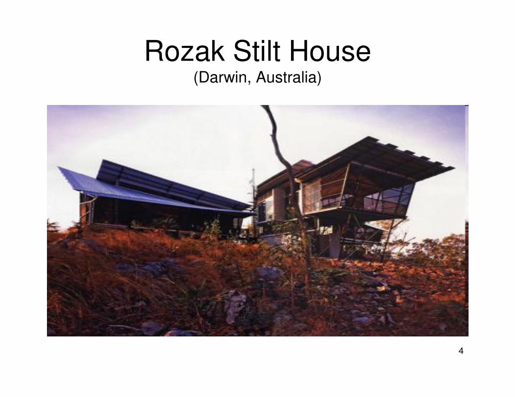
Rozak Stilt House (Darwin, Australia)

5

Luxury Villas in Pacific Islands

6

Natural Ventilation in Domestic Green Architecture

7

Natural Ventilation Multistory Buildings

Daytime stack effect Nighttime stack effect

Double facade Central atrium

8

Natural Ventilation in Commercial Buildings

Genzyme Center,

Cambridge MA

Corporate headquarters

biotechnology company

Designed from “inside – out”

9

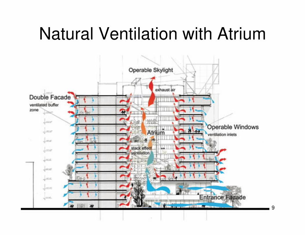
Natural Ventilation with Atrium

10

11

12

Natural Ventilation in Skyscrapers

City of Bristol Education Building - Skills Academy

Crystal Island Tower –

Norman Foster, Moscow

Gazprom Tower, St

Petersburg

Russia Tower – Norman

Foster, St. Petersburg

Encana Tower, Calgary,

Canada

13

Crystal Island “Volcano”

14

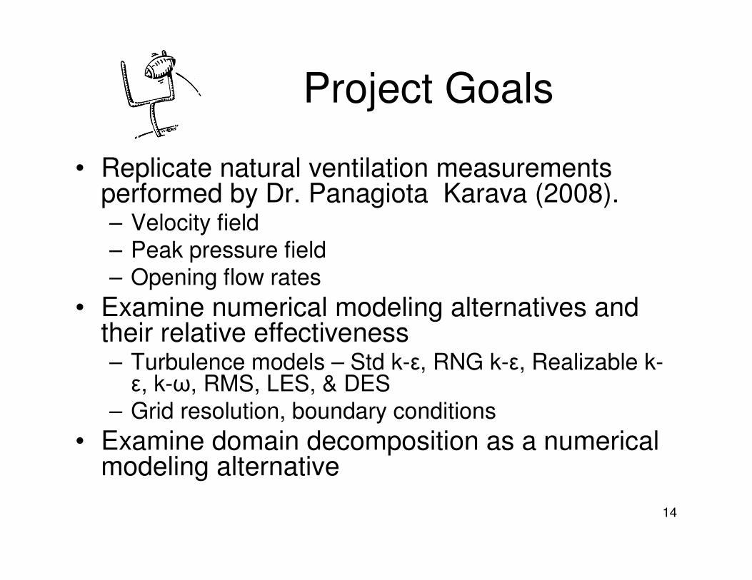
Project Goals

• Replicate natural ventilation measurements performed by Dr. Panagiota Karava (2008).– Velocity field

– Peak pressure field

– Opening flow rates

• Examine numerical modeling alternatives and their relative effectiveness– Turbulence models – Std k-ε, RNG k-ε, Realizable k-ε, k-ω, RMS, LES, & DES

– Grid resolution, boundary conditions

• Examine domain decomposition as a numerical modeling alternative

15

Karava Natural Ventilation Study

• Dr. Panagiota Karava, University of Western Ontario, – specialist in natural ventilation design.

• PhD Thesis: Airflow Prediction in Buildings for Natural Ventilation Design: Wind Tunnel Measurements and Simulation, Concordia University, 2008– Building Model 20 x 20 x 16 m high (1:200

scale ration), openings placed on different walls

– Simulated atmospheric boundary, p = 0.11

– Measurements with PIV & hot-film anemometry and fast-response pressure transducers

16

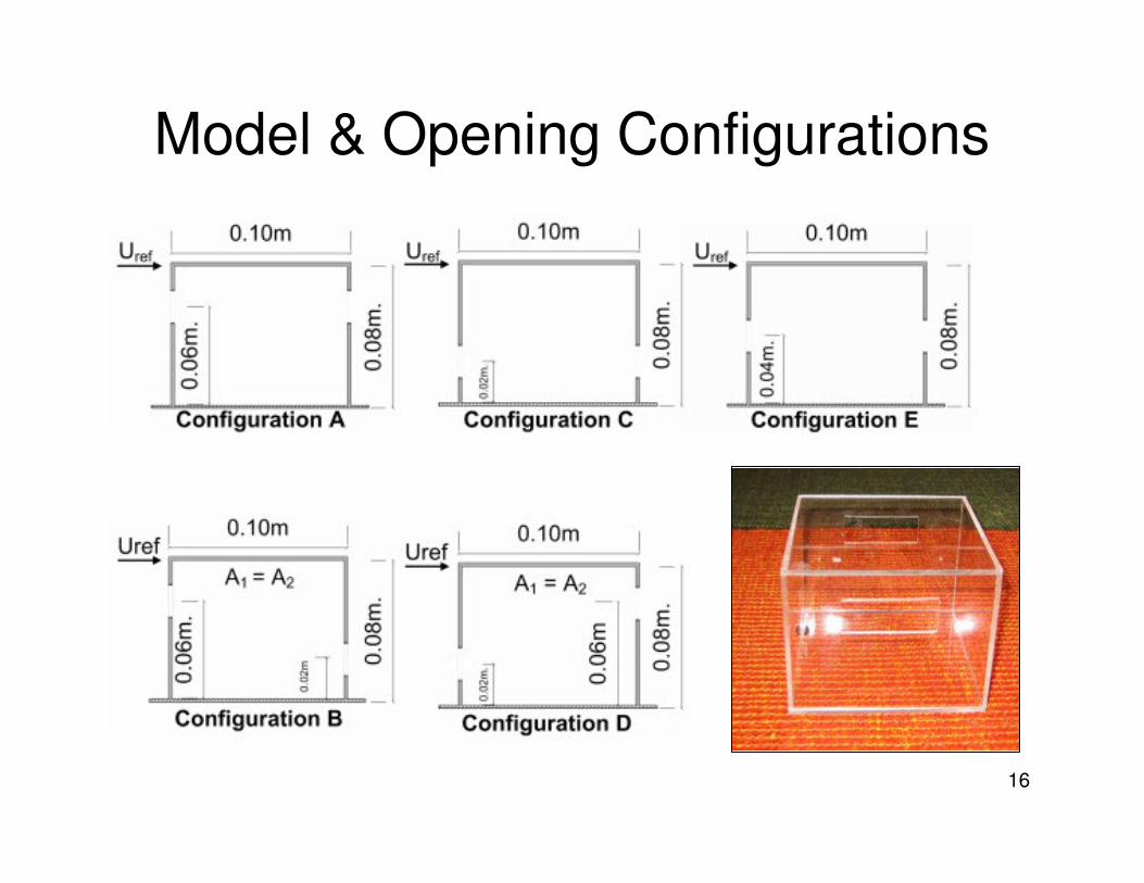
Model & Opening Configurations

17

PIV SystemHorizontal Plane Measurements Vertical Plane Measurements

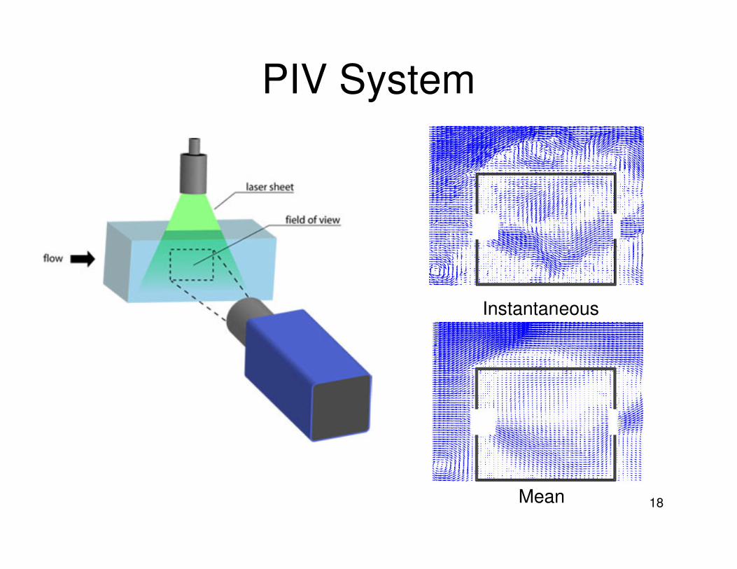
18

PIV System

Instantaneous

Mean

19

Numerical Model

• Domain size and flow conditions set to meet COST harmonization recommendations.

• Computational domain prepared with a combination of hexagonal and tetrahedral shapes totaling ~1 to 2 million cells. Cells adapted near walls to sizes less than 0.03 cm for the wind-tunnel scale model (8 x 10 x 10 cm)

• Wall boundaries had zero or 2 mm thickness.• Only configurations with wind normal to

openings considered.• All solutions obtained with the FLUENT 6.3 CFD

code.

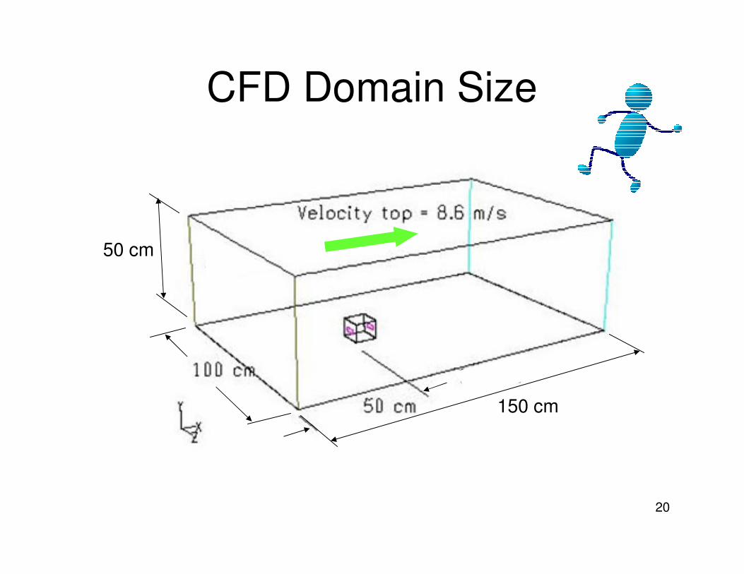
20

50 cm

150 cm

CFD Domain Size

21

Model Dimensions

A: 6 cm

C: 2 cm

E: 4 cm

2217

1.00

-

-

0.75

-

-

0.50

-

-

0.25

-

-

0.0

z/zg

1.00

-

-

0.75

-

-

0.50

-

-

0.25

-

-

0.0

z/zg

p = 0.11

Approach Flow Conditions

23

Flow field – Standard k-ε

Velocity Magnitude z = 50 cm Turbulent Intensities z = 50 cm

24

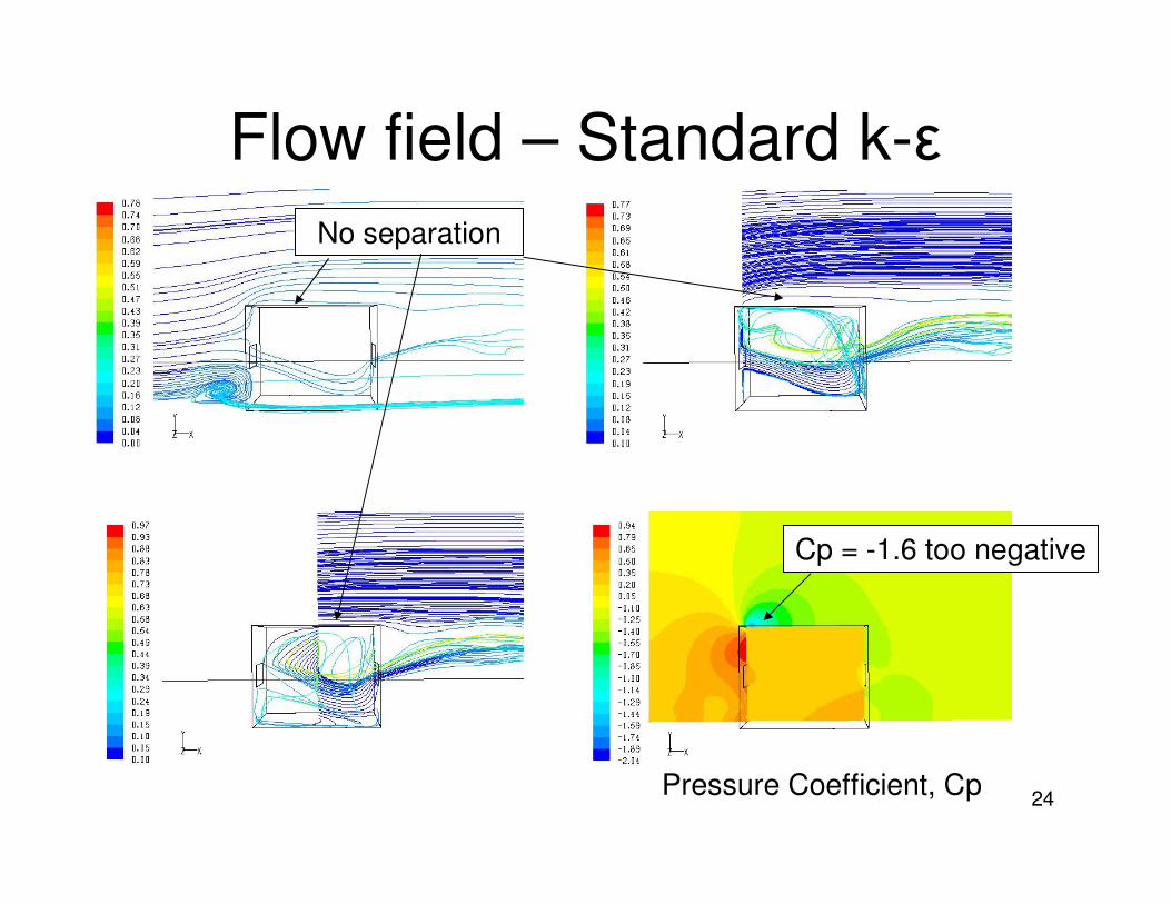
Flow field – Standard k-ε

Pressure Coefficient, Cp

No separation

Cp = -1.6 too negative

25

Path lines - Standard k-ε

26

Flow field – SST k-ω

Velocity Magnitude z = 50 cm Turbulent Intensities z = 50 cm

27

Flow field – SST k-ω

Cp = -1.4 too negative

No separation

Pressure Coefficient, Cp

28

Path lines – SST k-ω

29

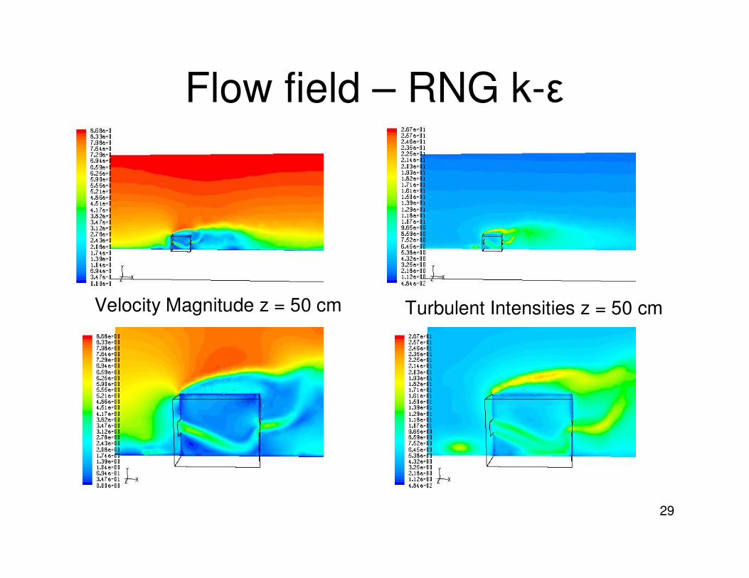
Flow field – RNG k-ε

Velocity Magnitude z = 50 cm Turbulent Intensities z = 50 cm

30

Flow field – RNG k-ε

Pressure Coefficient, Cp

Separation but no

reattachment

Cp = -0.53

31

Path lines – RNG k-ε

32

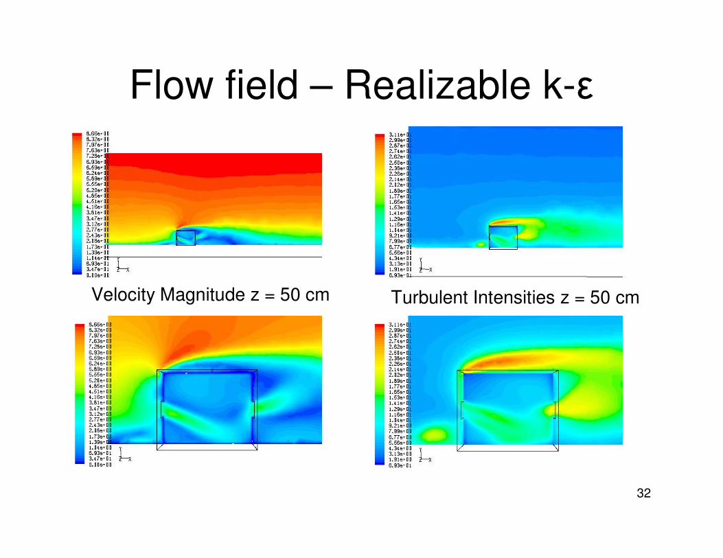
Flow field – Realizable k-ε

Velocity Magnitude z = 50 cm Turbulent Intensities z = 50 cm

33

Flow field – Realizable k-ε

Pressure Coefficient, Cp

Cp = -1.1 ok

Separation & reattach-

ment on roof

34

Path lines – Realizable k-ε

35

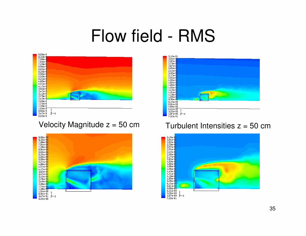
Flow field - RMS

Velocity Magnitude z = 50 cm Turbulent Intensities z = 50 cm

36

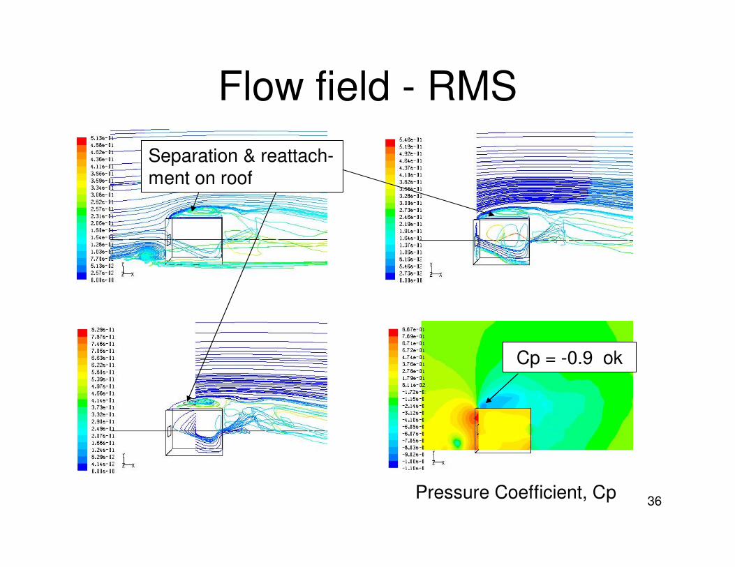
Flow field - RMS

Cp = -0.9 ok

Separation & reattach-

ment on roof

Pressure Coefficient, Cp

37

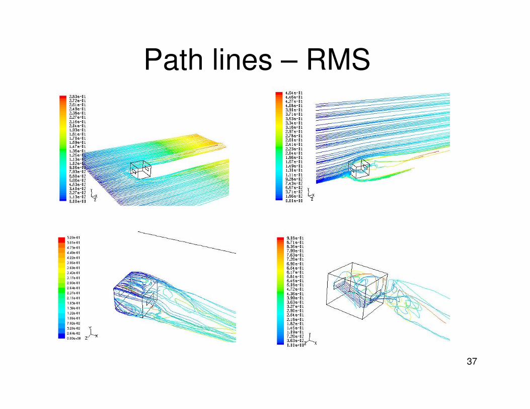
Path lines – RMS

38

Flow field – LES

Velocity Magnitude z = 50 cm RMS Velocity Magnitude z = 50 cmMean Velocity Magnitude z = 50 cm

39

Flow field – LES

Cp = -0.93 ok

Separation & reattach-

ment on roof

Pressure Coefficient, Cp

40

Path lines – LES

41

Flow field – LESFull field computation

42

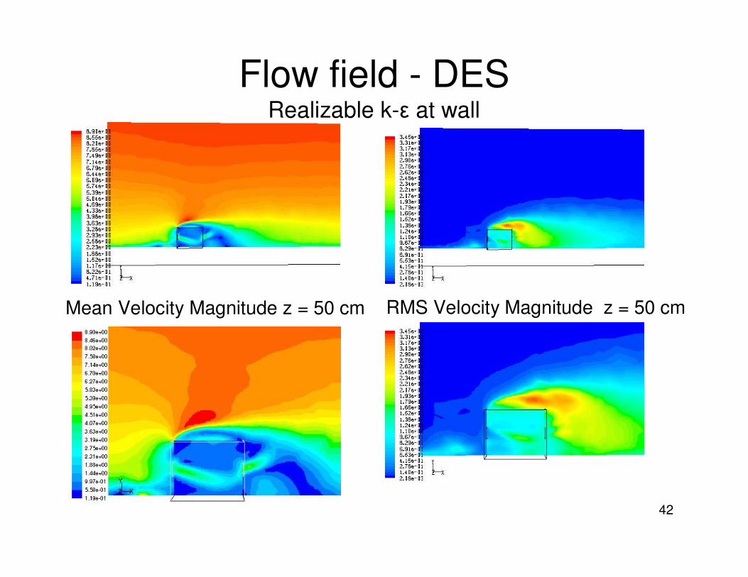
Flow field - DES Realizable k-ε at wall

RMS Velocity Magnitude z = 50 cmVelocity Magnitude z = 50 cmMean Velocity Magnitude z = 50 cm

43

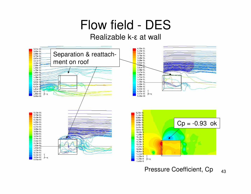
Flow field - DES Realizable k-ε at wall

Cp = -0.93 ok

Separation & reattach-

ment on roof

Pressure Coefficient, Cp

44

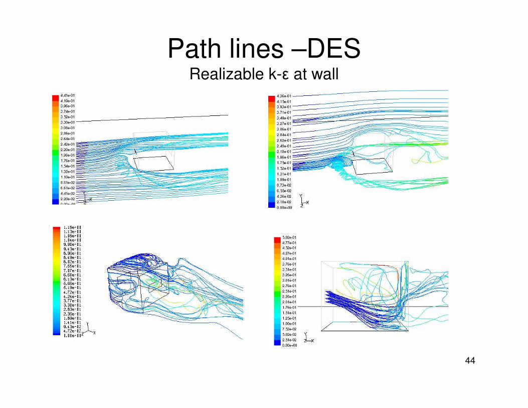
Path lines –DES Realizable k-ε at wall

45

Flow field DES

46

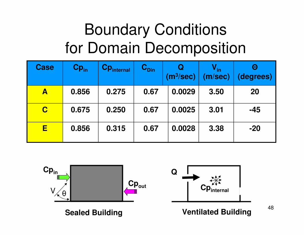
Domain Decomposition

• Kurabuchi et al. (2009) proposed one perform a full domain calculation around a sealed building, then calculate internal flows separately (fast)– Predict external flow over sealed building with CFD

– Note external pressures,

– Note adjusted internal pressure– Note tangential dynamic pressure at surface or θ

• Calculate Q and Cpinternal– Q = CDinAVH (Cpin – Cpinternal)

1/2…………...…Eq (1)

– Cpinternal = (Cpin + Cpout)/2…………………….Eq (2)

• Calculate internal flow using Q and Vtangential

47

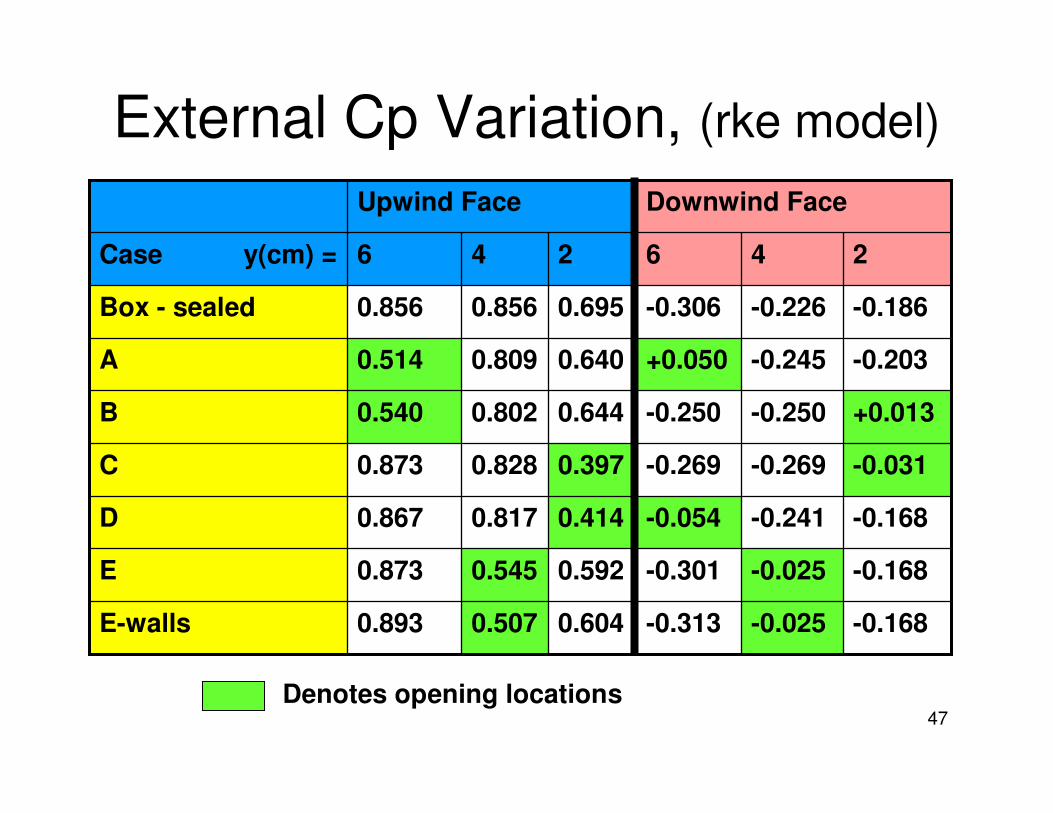
External Cp Variation, (rke model)

-0.168-0.025-0.3130.6040.5070.893E-walls

-0.168-0.025-0.3010.5920.5450.873E

-0.168-0.241-0.0540.4140.8170.867D

-0.031-0.269-0.2690.3970.8280.873C

+0.013-0.250-0.2500.6440.8020.540B

-0.203-0.245+0.0500.6400.8090.514A

-0.186-0.226-0.3060.6950.8560.856Box - sealed

246246Case y(cm) =

Downwind FaceUpwind Face

Denotes opening locations

48

Boundary Conditions for Domain Decomposition

-203.380.00280.670.3150.856E

-453.010.00250.670.2500.675C

203.500.00290.670.2750.856A

Θ

(degrees)

Vin

(m/sec)

Q

(m3/sec)

CDinCpinternalCpinCase

θV

Cpin

Cpout

Q

Cpinternal

Sealed Building Ventilated Building

49

Vector Section – Case A: rkePIV Measurements Full domain CFD calculation

Domain Decomposition

Vena Contracta

No Vena Contracta

50

Flow field – LESDomain decomposition computation

51

Vector Section – Case C: rkePIV Measurements Full domain CFD calculation

Domain Decomposition

52

Flow field – LESDomain decomposition computation

53

Vector Section – Case E: rkePIV Measurements Full domain CFD calculation

Domain Decomposition

54

Flow field – LESDomain decomposition computation

55

Velocity Ratio – VX/VH

CASE A CASE C

CASE E

PIV A, C & E

CFD full domain

CFD decomposition,

various angles

56

External Flow Characteristics

-1.220-0.2350.535RkeD

-1.090-0.2180.545RkeC

-1.280-0.2380.587RkeB

-0.930-0.2270.568RkeA

-0.940-0.1600.720KaravaBox

-0.825-0.2540.595RkeBox

-0.931-0.2520.627DESE

-0.931-0.2870.611LESE

-0.868-0.3320.581RMSE

-1.400-0.2410.829k-ωE

-0.530-0.2570.635RNGE

-1.180-0.2430.556RkeE

-1.600-0.2660.570SkeE

Cprooftop

Minimum

Cpdownwind

Average

Cp upwind

Average

Turbulence

Model

Case

Discounting Ske, RNG & k-ω, then average upwind Cp = -0.594 ±

0.027, and average downstream Cp = -0.273 ± 0.037. Deviations are

less than AIJ Working Group study in multiple wind tunnels.

Cdrag = (Cpupwind –Cpdownwind)Average. Drag coefficient for sealed

building is 0.85, whereas drag coefficient for paired openings sets is

0.80 ± 0.03. Drag coefficients for Case E over various turbulence

models ranged from 0.80 to 1.07.

57

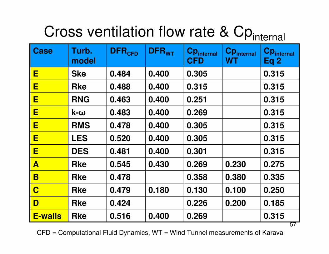
Cross ventilation flow rate & Cpinternal

0.3150.2690.4000.516RkeE-walls

0.1850.2000.2260.424RkeD

0.2500.1000.1300.1800.479RkeC

0.3350.3800.3580.478RkeB

0.2750.2300.2690.4300.545RkeA

0.3150.3010.4000.481DESE

0.3150.3050.4000.520LESE

0.3150.3050.4000.478RMSE

0.3150.2690.4000.483k-ωE

0.3150.2510.4000.463RNGE

0.3150.3150.4000.488RkeE

0.3150.3050.4000.484SkeE

Cpinternal

Eq 2

Cpinternal

WT

Cpinternal

CFD

DFRWTDFRCFDTurb.

model

Case

CFD = Computational Fluid Dynamics, WT = Wind Tunnel measurements of Karava

58

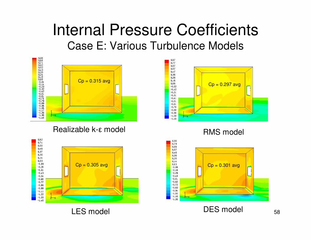
Internal Pressure Coefficients Case E: Various Turbulence Models

RMS model

Cp = 0.297 avg

LES model

Cp = 0.305 avg

DES model

Cp = 0.301 avg

Realizable k-ε model

Cp = 0.315 avg

59

Internal Pressure Coefficients Case A-D: Realizable k-ε Model

Case A

Cp = 0.269 avg

CpKARAVA = 0.230

Case B

Cp = 0.358 avg

CpKARAVA = 0.380

Case C

Cp = 0.130 avg

CpKARAVA = 0.100

Case D

Cp = 0.226 avg

CpKARAVA = 0.200

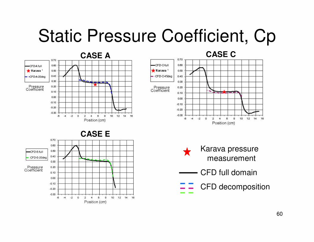
60

Static Pressure Coefficient, CpCASE A CASE C

CASE E

Karava pressure

measurement

CFD full domain

CFD decomposition

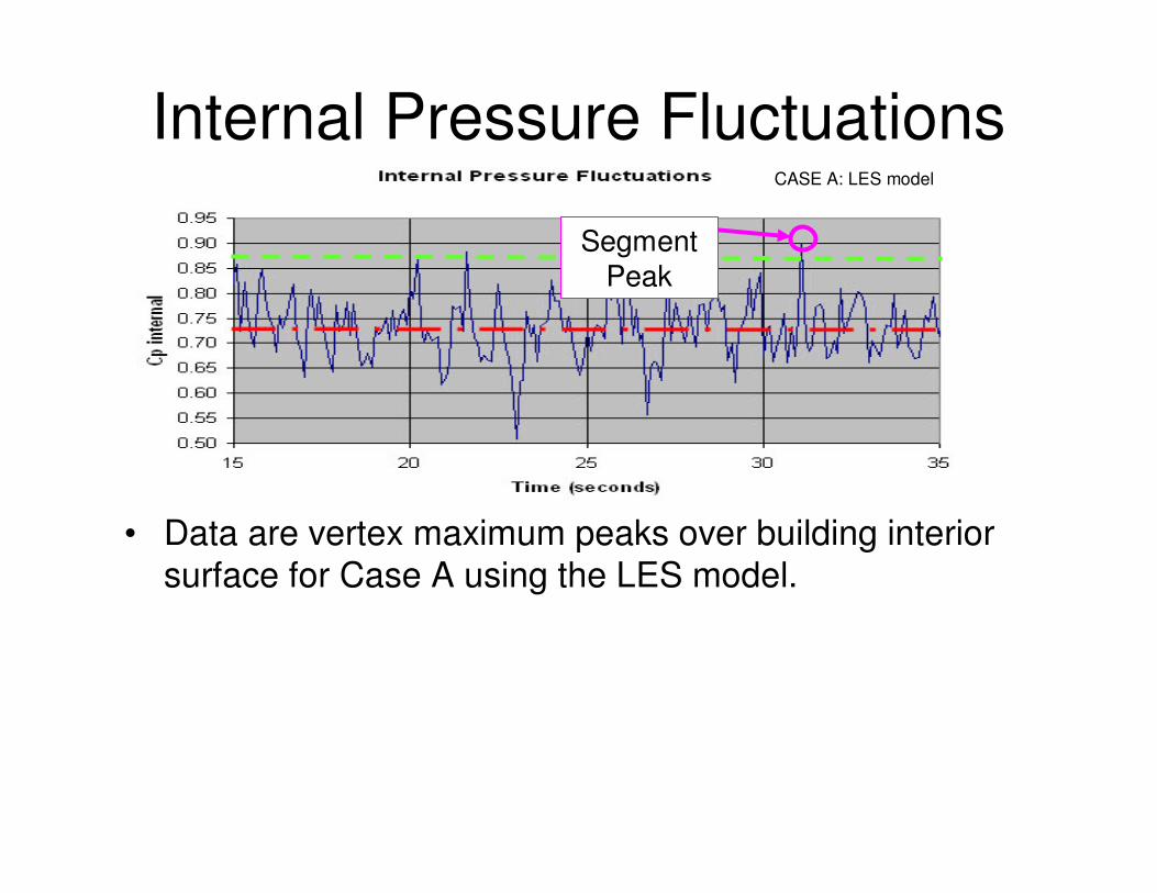
61

• Data are vertex maximum peaks over building interior

surface for Case A using the LES model.

• Average of all peaks = 0.725

• Average of segment peaks = 0.870 taken over

thirty 100 second sampling intervals

• Cppeak = Cpmean + g * CpRMS where g ≈ 5………Eq (3)

Internal Pressure FluctuationsCASE A: LES model

Segment

Peak

62

Peak & mean internal pressure coefficients

____0.882 (0.713)

0.7490.0860.319E

0.400.1000.978

(0.288)

0.2390.0260.109C

0.750.2300.870 (0.339)

0.4580.0610.153A

Cppeak

WT

Cpmean

WT

Cppeak

CFD TS#

Cppeak

Eq 3

Cprms

CFD

Cpmean

CFD

Case

CFD = Computational Fluid Dynamics,

WT = Wind Tunnel measurements of Karava, and

TS = Time Series

# Numbers are vertex maximum peaks over building interior surface

# Numbers in (italics) are peaks over five selected interior points

63

Conclusions

• CFD model replicated wind tunnel data– Internal flow field, magnitude and directions

– Internal Ux/UH profiles between openings

– Internal Cp profiles between openings

– Internal character of peak pressure variations

– External front, rear & roof pressure values

• Domain decomposition also replicated wind tunnel data within experimental and numerical uncertainty.

64

The End