cfd techniques for mixing and dispersion of desalination ... · april 2014 cfd techniques for...
TRANSCRIPT

April 2014
CFD techniques for mixing and dispersion of desalination and other marine discharges
ICDEMOS, Muscat, Sultanate of Oman, 2014
David Robinson, Matthew Wood, Matthew Piggott & Gerard Gorman

© HR Wallingford 2014
Content
Background and motivation CFD: a tool for dispersion modelling Preliminary results Planned work
April 2014
© HR Wallingford 2014
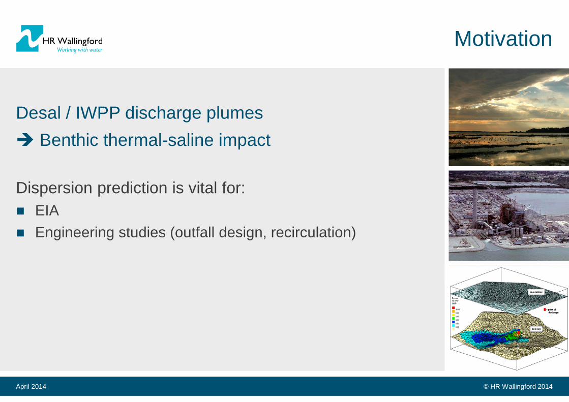
Motivation
Desal / IWPP discharge plumes Benthic thermal-saline impact Dispersion prediction is vital for: EIA Engineering studies (outfall design, recirculation)
April 2014

© HR Wallingford 2014
HR Wallingford in Oman
April 2014

© HR Wallingford 2014
Far-field dispersion
Model coupling
Near-field dilution
(mixing zone)
Dispersion modelling approaches
April 2014

© HR Wallingford 2014
Validated procedure
April 2014
Coupled studies are common
HR Wallingford framework: “Dense Jet Assessment Procedure”, Wood & Mead (2008)
Validated against newly available mid-/far-field data: “Validation of computational models for hypersaline and other dense marine discharges”, Wood et al, (2014)

© HR Wallingford 2014
Benefits & drawbacks
Benefits: Methods generally work well for smaller discharges:
Simple exchanges of mass & momentum Relatively quick to implement
Drawbacks Plume interactions / neighbouring facilities :
2-way exchange of pollutant concentrations is challenging
Potential solution: CFD Computing power increases Adaptive meshing techniques Seamless coverage of the entire domain
April 2014
Barka
Sohar

© HR Wallingford 2014
CFD
History – near-field Fluidity:
Open-source, developed by Imperial Navier-Stokes on 3D unstructured meshes Discretisation: Finite element & control volume Mesh adaptivity
Key differentiator – multi-scale:
3D CFD model + efficient coastal flow modelling system
Used to simulate ocean and tidal flows
April 2014

© HR Wallingford 2014
PhD research
Long-term goals: Extend Fluidity’s multi-scale capabilities a fully integrated CFD hydrodynamic & pollutant dispersion model
First stage: Explore near-field abilities
Horizontal buoyant jet Angled dense jet
Compared predictions with published laboratory data, or validated integral models.
April 2014

© HR Wallingford 2014
Near-field test cases
April 2014
Parameter Horizontal buoyant jet Angled dense jet
Inlet diameter (mm) 9.4 3.3 Densimetric Froude number, F 10.7 21.3 Reynolds number 6000 2500 References for comparison CorJet integral model Experimental data
Parameters for comparison • Centreline trajectory • Mean axial velocity decay
• Centreline terminal rise height • Bottom impact distance • Minimum impact dilution
Zt
Si Xi

© HR Wallingford 2014
Numerical methods
Unstructured tetrahedral elements Turbulence:
k-ε V-LES
Adaptive time-stepping and meshing
April 2014

© HR Wallingford 2014
Horizontal buoyant jet
April 2014

© HR Wallingford 2014
Horizontal buoyant jet
April 2014
Centreline trajectory
Centreline velocity decay

© HR Wallingford 2014
Angled dense jet
April 2014

© HR Wallingford 2014
Angled dense jet
April 2014
k1 = zt/dF k2 = xi/dF k3 = Si/F Zeitoun et al. (1972) - 3.19 1.12 Roberts et al. (1997) - 2.4 1.6 +/- 0.12 Nemlioglu & Roberts (2006) - 3.25 1.7 Cipollina et al. (2005) 1.77 2.25 - Kikkert et al. (2007) 1.6 2.72 1.81 Papakonstantis et al. (2011a and 2011b) 1.68 2.75 1.68 +/- 0.1
Terminal rise
height
Impact distance
Impact dilution

© HR Wallingford 2014
Summary
HR Wallingford uses a validated coupled modelling procedure involving Hydrodynamic models Near-field models
Future will involve more CFD
Preliminary work with Imperial College is encouraging:
Buoyant jet compares well (trajectories and dilutions) Dense case requires mesh refinement
Next steps of PhD: Adapt mesh to far-field Range of ambient currents Multiport diffusers
April 2014

© HR Wallingford 2014
Thank you!
Matthew Wood Principal Scientist HR Wallingford [email protected]
David Robinson Imperial College London [email protected]
January 2014 Page 17