cfd-based compartmental modeling of single phase …elektron.tmf.bg.ac.rs/mre/day 5/5.a.4 -...
TRANSCRIPT
1
CFD-Based Compartmental Modeling of Single Phase Stirred
Tank Reactors
Debangshu Guha, M.P. Dudukovic and P.A. Ramachandran
Chemical Reaction Engineering Laboratory, Washington University in St.
Louis, St. Louis, MO 63130
S. Mehta and J. Alvare
Air Products and Chemicals Inc., Allentown, PA 18195
Abstract
Mechanically agitated reactors are widely used in variety of process industries.
Traditional designs assume perfect mixing which often fails to predict the
performance of large scale industrial reactors. The effect of mixing becomes
pronounced when the time scales of some of the reactions are small compared
to the time scale of mixing. The objective of this work is to predict the
influence of mixing on the performance of stirred tank reactors by developing
a compartmental model that incorporates the flow field simulated by CFD.
This enables the coupling of the flow field, turbulent mixing and kinetics in an
appropriate way and bridges the existing gap between CFD and
phenomenological models.
Topical Heading: Reactors, Kinetics and Catalysis
Keywords: Stirred tank, Single Phase, Mixing, CFD, Compartmental Model

2
Introduction:
Traditional design of mechanically agitated reactors, which are widely used in
variety of process industries, is based on the assumption of perfect mixing.
This assumption is only justified when all the reaction time scales are much
larger than the mixing time scale. It often fails because perfect mixing at all
length scales can never be achieved and concentration gradients do exist
within the reactor over finite distances and times. This has serious
consequences for scale up of multiple reaction systems where some of the
reaction time scales are small compared to the time scale of mixing. Since
chemical reactions are molecular events, the product distributions can be
severely affected by the concentration inhomogeneities within the reactor. As
a result, the formation of undesired products can increase significantly thereby
leading to increased generation of wastes.
Mixing in a stirred tank reactor takes place through convection (at
larger length scales in the inertial subrange; commonly referred to as
macromixing), coarse-scale turbulent exchanges (at intermediate length scales
larger than the Kolmogorov scale; commonly called mesomixing), as well as
by deformation of fluid elements followed by molecular diffusion (at smaller
length scales below the Batchelor scale; commonly described as
micromixing)1. In the completely turbulent regime (Reynolds number for
impeller, 410Re >imp ) the macromixing effect on the reactor performance
depends highly on the flow field that exists within the reactor. Hence, detailed
Correspondence concerning this article should be addressed to M.P.Dudukovic

3
flow descriptions are needed to describe the mixing effects and predict the
performance in a stirred tank reactor.
Mixing effects in stirred vessels have been traditionally addressed
using phenomenological models. These models provide analysis of the effects
of mixing on the product distribution and selectivity of industrial reactions in
stirred reactors. Common phenomenological models include the Segregated
flow/ Maximum mixedness models, the Interaction by Exchange with the
mean (IEM) model2, the Engulfment Deformation Diffusion (EDD) model3,
and more recently the Population Balance model4. These models attempt to
describe the effect of micromixing on the reactor performance, but none of
them account for the detailed flow description within the reactor
(macromixing). The other usual approach is that of compartmental modeling,
which essentially attempts to describe the macromixing effects on the reactor
performance and also accounts for certain level of mesomixing through the
inclusion of the exchange coefficients. An example of this approach is the
Network of Zones model5,6, which does account for the prevalent flow field
inside the reactor. This model, however, depends on the available literature
correlations for the impeller pumping flow (the flow number) which are
needed to map the flow field in the system. It has been shown that the
uncertainties in the estimation of the flow number (which varies about 30-50%
when based on different literature correlations) can result in significant
uncertainties in the model predictions7. Mesomixing is mimicked in the
Network of Zones model by the use of exchange flows between compartments
which are taken as a fraction of the main flow through the compartment. The
number of compartments and the fractions selected for estimation of the

4
exchange flows serve as model parameters and are generally selected
arbitrarily. However, in spite of its limitations, this approach has been shown
to capture the essential features of macromixing in stirred vessels operating in
both batch8 and semi-batch9 modes. The qualitative comparison of 3-D
visualizations of passive tracer mixing using a colored dye shows reasonable
agreement with the model predictions8. More recently, CFD has emerged as
an alternative for the solution of reactive flow problems which can be used to
solve the flow field as well as the concentration field simultaneously (or
separately) in a stirred vessel10,11,12. But the CFD solutions can become
computationally intensive for industrial reactions and reactors where the
number of components involved might be significantly large and the vessels
are huge. This can be of concern for on-line prediction of product distribution
and hence, such an approach will not be suitable for process optimization and
model based advanced control.
An improved methodology (in terms of reduced computational expense
and time) can be devised if the CFD solution for the flow in the reactor is used
along with the phenomenological models, thereby decoupling the flow and the
kinetics of the system but still accounting for the effect of the hydrodynamics
on the mixing behavior of the system. There have been some modeling efforts
along these lines recently for many types of reactors including stirred
tanks13,14,15 and bubble columns16. These models have been shown to produce
reasonable predictions at much lower computational cost. This makes them
suitable for optimization of product distribution, formulation of pollution
prevention strategies and advanced model based control. The simple two-
compartment model13, however, is still a significant simplification of the flow

5
description within the reactor and therefore it is unlikely that the model will
capture the effect of different feed locations on reactor performance. Akiti and
Armenante (2004)15 used the Volume of Fluid (VOF) approach to track the
reaction zone and solved the reactive flow problem using the Engulfment
model3, where the engulfment parameter is calculated using the averaged
turbulent parameters (k and ε) in the reaction zone. Though the qualitative
trends for different feed locations are captured, quantitative comparison shows
discrepancies with the experimental results. The work presented here attempts
to develop the CFD-based compartmental approach, in which the complete
CFD solution of the flow and turbulence parameters provides the input for the
compartmental mixing model. A scheme to calculate the number of
compartments necessary for a given reactive system has also been devised
based on the time scales associated with the process. The application of the
model for single phase systems is shown in this paper but it can be extended to
model multiphase systems as well (e.g. gas-liquid or liquid-solid systems).
However, it is important to recognize that this model can only account for
macromixing and mixing due to turbulent dispersion but ignores micromixing
effects on reactor performance. The condition for which micromixing effects
can be ignored depends on micromixing time scale compared to reaction time
scale as discussed later in the text.
This paper is organized as follows: the detailed model for turbulent
reactive flows is described, followed by the model reduction to obtain the
compartment level equations along with the assumptions involved. Then the
discretization strategy and incorporation of CFD solution into the
compartmental framework is described. The next section provides the results

6
and discussions for mixing with and without reactions. Finally, the
conclusions of this work are outlined.
Detailed Model for Turbulent Reactive Systems:
The mass balance equation for any component c in the reactor is given by17
ci
cm
i
ci
c Rxc
Dxc
ut
c+
∂∂
=∂∂
+∂∂
2
2
…………….. (1)
Reynolds averaging equation (1) by decomposing the concentration as
'ccc ccc += and the velocity as '
iii uuu += results in
'2
2''
cc
i
cm
i
ci
i
ci
c RRxcD
xcu
xcu
tc
++∂∂
=∂∂
+∂∂
+∂∂ ………………. (2)
Rendering equation (2) dimensionless by using a characteristic length
scale L, velocity scale U0 and concentration scale C0 we get (* indicates
dimensionless quantities),
'**
2*
*2
0*
'*'*
*
**
*
*
cc
i
cm
i
ci
i
ci
c RDaRDaxc
LUD
xcu
xcu
tc
++∂∂
=∂
∂+
∂∂
+∂∂ …………… (3)
The second term on the LHS of equation (3) accounts for convection due to
the mean flow. The third term accounts for dispersion caused by the
fluctuations. The Reynolds averaged reaction term contains the contributions
from the mean reactant concentrations (*cR ) and the mean of the cross terms of
the fluctuating concentrations ( '*cR ). Damkohler number, Da, is the ratio of the
convection time scale to the reaction time scale ( ))(/()/( 000 CRCULDa = ).
The first term on the RHS accounts for the contribution from molecular
diffusion. 0LU
Dm is the ratio of the convection time scale to the diffusion time

7
scale, i.e. inverse of the Peclet number, Pe. For completely turbulent flows at
high Reynolds number for liquid phase systems Pe >> 1 (since Re>>1 and Sc
>> 1) and the contribution of molecular diffusion can be safely neglected.
However, the scalar-flux term (dispersion) and the second part of the reaction
term ( '*cR ) need to be closed to solve the system of equations.
The scalar flux term is commonly closed using the gradient diffusion
model18 which can be written as
*
*
0
'*'*'' ,i
ctci
i
ctci x
cLUD
cuorxcDcu
∂∂
−=∂∂
−= …..…….(4)
where Dt is defined as the turbulent diffusivity, or the eddy dispersion
coefficient, which varies from region to region within the reactor. 0LU
Dt is the
ratio of the convection time scale to the dispersion time scale (inverse of the
dispersion Peclet number), i.e. a product of the 1−TSc (turbulent Schmidt
number) and 1Re−t (
tt
LUν
0Re = ).
The contribution from the fluctuating concentration in the reaction
term ( '*cR ) is small for slow reactions (Da<<1), where the turbulent mixing
will occur before the reaction can take place18. In other cases the reaction term
can be closed using a PDF description of the scalar field. The advantage of
this method is that the total contribution to the reaction term can be directly
calculated from the composition PDF18. An example which uses the presumed
PDF method is the Turbulent Mixer model1,19 which characterizes the mixture
structure by solving the mixture fraction and the variance (decomposed into

8
different components) equations for an inert tracer. The details of the different
closures available for the reaction term can be found elsewhere20.
This differential model (equation 3) can be solved along with the
Navier-Stokes equations to compute the concentration field within the reactor.
Commercially available CFD packages like FLUENT have codes to solve
these equations based on the finite volume approach. However, as mentioned
earlier, this can become computationally intensive for multiple reactions with
complex chemistries. In such cases model reduction into compartments can be
useful.
Model Reduction and Compartment Level Equations:
The compartmental modeling approach divides the entire reactor into a
number of connected, well-mixed compartments as shown in Figure 1. Model
reduction for this work is then obtained by volume averaging equation (3) over
a defined compartment (a finite control volume V), which yields
∫∫∫∫ ∫ +=∂
∂+
∂∂
+V
cV
c
V i
ci
V V i
cic dVRDadVRDadV
xcu
dVxcudVc
dtd '**
*
'*'*
*
***
* ...…..(5)
Using the Divergence Theorem and substituting equation (4) for '*'*ci cu ,
equation (5) is modified to,
∫∫∫∫ ++∂∂
=+⟩⟨
Vc
V
c
S i
ci
t
S
ciic dVRDadVRDadS
xcn
LUD
dScundt
cdV '**
*
*
0
**
*
*
)( …..(6)
where ⟩⟨ *cc is the volume averaged concentration in the control volume
defined as VdVccV
cc ∫=⟩⟨** . The second term on the LHS of equation (6) can
9
be written as ∫ ∑=
⟩⟨⟩⟨=S k
kkmckmcii ScudScun6
1
*,
***)( , where, kmu ⟩⟨
* is the surface
average velocity and kmcc ⟩⟨*
, is the mixing-cup average (or volumetric flow
rate average) concentration on surface k of the compartment defined as
∫
∫=⟩⟨
k
k
Sk
Skii
kmdS
dSunu
*
* and
∫
∫=⟩⟨
k
k
Skii
Skcii
kmc
dSun
dScunc *
**
*,
)(
Note that the mixing-cup average concentration ( kmcc ⟩⟨*
, , for all k) is equal to
the volume averaged concentration ( ⟩⟨ *cc ) only when there is no concentration
gradient in the volume element.
The first term on the RHS (dispersion term) of equation (6) denotes
mixing due to eddy transport (mesomixing) across the cell faces. This can be
written as ∫ ∑=
⟩∂∂⟨
⟩⟨=
∂∂
S kkk
i
ckt
i
ci
t Sxc
LUD
dSxcn
LUD 6
1
*
0
*
0
, where, ktD ⟩⟨ is the surface
average turbulent diffusivity and ki
c
xc⟩
∂∂⟨
*
is the surface average gradient of the
concentration on surface k of the compartment defined as
∫
∫=⟩⟨
k
k
Sk
Skt
ktdS
dSD
D and ∫
∫ ∂∂
=⟩∂∂⟨
k
k
Skt
Sk
i
cti
ki
c
dSD
dSxcDn
xc
*
*
Note that k
i
mck
i
c
xc
xc
∂⟩∂⟨
=⟩∂∂⟨
*,
*
only when there is no concentration gradient on
the surface of the compartment and ki
c
ki
c
ki
mc
xc
xc
xc
Δ⟩⟨Δ
=∂
⟩∂⟨=
∂⟩∂⟨ ***
, when there is
no concentration gradient within the compartment volume as well. In this

10
work, the compartments are assumed to be perfectly mixed which can be
justified when the size of the compartments is small and the local Da in each
compartment is kept smaller than 1. With this assumption, equation (6)
becomes,
∫∫∑∑ ++Δ
⟩⟨Δ⟩⟨=⟩⟨⟩⟨+
⟩⟨
== Vc
V
ck
kki
ckt
kkkckm
c dVRDadVRDaSxc
LUD
Scudt
cdV '**6
1
*
0
6
1
**
*
*
…………..(7)
Some comments on the role of the dispersion term are warranted here.
Note that the inverse of the dispersion Peclet number appearing in equation (7)
can be written as
0
1111
0
ReReU
UScScLUD local
localTtTkt −−−− ==⟩⟨
where Ulocal is the characteristic velocity defined for a particular compartment
and Relocal is the local Reynolds number based on that velocity
(t
locallocal
LUν
=Re ). Turbulent Schmidt number, TSc , is taken as 0.8 for all
cases. In the regions far from the impeller, localRe and localU are both small
and the product 0
11 ReU
USc local
localT−− can be of O(1). In such a case, dispersion
will play a significant role on the predicted results. On the other hand, near the
impeller, the local Reynolds number is large ( 1Re−local <<1) and the ratio
0UU local is of O(1). In those regions the relative importance of this term is small
and convection dominates the mixing behavior of the system. This has been
shown in the results as well, where the inclusion of the dispersion term is
11
important when the reactant feed point is far from the impeller but is not
necessary when reactant feeding is close to the impeller.
The second term on the RHS of equation (6) is the reaction term due
to the mean concentration, where, )(**cc cfR = . When no concentration
gradients exist within a compartment this can be written as
VcRdVcR cc
V
cc )()( ****⟩⟨=∫ . The third term on the RHS (contribution from the
mean of the cross terms) is neglected in this work based on the fact that the
local Da in each compartment is kept smaller than 1 when the reactor is
discretized into compartments. Equation (7) then gets modified to
VcRSxc
LUD
Scudt
cdVcc
kk
ki
ct
kkkckm
c )( **6
1
*
0
6
1
**
*
*
⟩⟨+Δ
⟩⟨Δ⟩⟨=⟩⟨⟩⟨+
⟩⟨ ∑∑==
………….(8)
Equation (8) represents the mass balance for any component c in a
compartment in dimensionless form. In terms of dimensional variables
equation (8) can be represented as
……………… (9)
where, ∑=
=RN
mmmcc rR
1ν ; =RN number of reactions; =mr intrinsic rate of the
m-th reaction; mcν = stoichiometric coefficient and )1( −iexk = exchange
coefficient at the (i-1) face of the compartment (i,j,k) which is related to Dt as
kjickji
ckji
caxk
ex
kjic
kjicax
kex
kjic
kjic
jex
kjic
kjic
jex
kjic
kjic
irad
iex
kjic
kjic
irad
iex
kjiaxax
kjic
kjikjic
kjirad
irad
kjic
kjiaxax
kjic
kjikjic
kjirad
irad
kjic
kjic
kji
VRccSk
ccSkccSkccSk
ccSkccSkuScuSc
uScuScuScuScdt
dcV
,,1,,,,)1(
1,,,,)1(,1,,,)1(,1,,,)1(
,,1,,)1(,,1,,1)1(,,,,,,,,
,,,,1,,1,,,1,,1,,,11,,1,,
,,
)(
)()()(
)()(
+−−
−−−−−−
−−−−−−
−++=
++
−−++−−
++−−−
−−−−−−−
θθ
θθ
θθ
12
shown later. Equation (9) is the final compartment level model equation used
in this work.
Compartmental Model Inputs from CFD:
The CFD-based compartmental model consists of the following steps. The
complete CFD solution of the flow field is first obtained in the entire tank. The
next step is to determine the required number of compartments depending on
the time scales of the reactions studied. This is discussed in the next section.
The first six terms on the RHS of equation (9) account for the transfer of
component c by the bulk mean flows which are obtained by averaging the
complete CFD solution over the faces of the defined compartments. The next
six terms in the equation account for the transfer of mass due to turbulent
dispersion. The exchange coefficient is estimated from the turbulent
diffusivity averaged over the faces of the compartment as indicated later in the
text.
Compartment Discretization scheme:
The discretization scheme followed in this work has the following objective.
Given the kinetics of a reactive system, the compartments are created in such a
way that the overall local residence time of the liquid in a compartment is less
than the characteristic reaction time scale, i.e.
rxniin
i tQV
<,
…………….. (10)
where iV is the volume of the i-th compartment, iinQ , is the sum of all the inlet
flows to the i-th compartment and rxnt is the characteristic reaction time scale.
13
This ensures that significant concentration gradients do not develop within a
compartment due to reaction (ensures that in each compartment 1<Da ) and
hence compartments can be assumed to be macroscopically well-mixed.
To achieve the overall objective, discretization is done independently
in each coordinate direction by choosing a velocity profile along that direction.
The scheme involves the following steps:
• Selecting an appropriate velocity profile for discretization in each of
the coordinate direction, i.e. axial, radial and angular.
• Discretization along each coordinate direction is performed so that in
each direction the individual criterion is met, i.e.
rxnavg
i tv
x<
Δ …………… (11)
where avgv is the average velocity between locations i and i+1.
Note that independent discretization in each coordinate direction
essentially ensures that equation (10) is satisfied for about one-third of the
actual reaction time scale. This follows from the scaling argument presented
below. Figure 2 shows a compartment of dimensions xr , xz and xθ, and three
characteristic velocity components vr, vz and vθ through the compartment in the
three co-ordinate directions, respectively. For the given compartment
)14.......(..........~
)13(.................~)12......(............~
θ
θ
θ
θθθ
θθθ
θ
xv
xv
xv
xxxxxvxxvxxv
VQ
xxvxxvxxvQxxxV
z
z
r
r
zr
zrrzzr
zrrzzr
zr
++=++
++

14
Now, if the discretization is carried out in each direction independently
(without accounting for the contribution of the flow from the other two
directions) we have
rxnr
r tvx
< , rxnz
z tvx
< and rxntvx
<θ
θ
which then implies that
)15..(..........3
,
3
rxn
rxn
tQVor
tVQ
<
>
Therefore, a reaction time scale rxnrxn tt 3~′ can be used for discretization, still
satisfying the overall criterion given by equation (10).
Selecting the velocity profile:
To select the axial velocity profile for discretization, circumferentially-
averaged axial velocity plots ( zvsvz . ) are obtained at different radial positions
in the reactor. An average axial velocity is calculated for each of the profiles
as
p
z
rz N
vv i
i
∑= ………….. (16)
where izv is the velocity at any given point in the profile and Np is the total
number of points. The average velocity obtained using equation (16) at each of
the radial locations is compared and the profile that has the smallest value of
the mean velocity is chosen for discretization. If equation (11) can be satisfied
for a plane which has the smallest average flow, it would satisfy the criterion
15
at other planes also where the average flows are larger (the compartment
length ixΔ remaining same).
The same procedure is followed to select the radial and tangential
velocity profiles by obtaining circumferentially-averaged radial and tangential
velocity plots ( rvsvrvsvr .&. θ ) at different axial locations. The profiles with
the smallest averages are chosen for discretization.
Discretization:
The number and location of the axial compartments is obtained using the
selected axial velocity profile. Given an axial location iz (Figure 3) and the
corresponding velocity izv , , we need to find a location 1+iz such that
rxn
iziz
ii tvv
zz<
+
−
+
+
,1,
1
21
………… (17)
Since the velocity profile is known, 1+iz can be obtained by iteration so that the
above criterion is satisfied.
The same procedure is followed to determine the number and location
of the radial compartments using the radial velocity profile. The angular
direction is divided evenly and the number of compartments can be obtained
as
⎥⎥⎦
⎤
⎢⎢⎣
⎡=
rxni
i
tvr
N,
2max
θθ
π …………. (18)
where iv ,θ is the tangential velocity at ir in the selected velocity profile.
This methodology is, however, conservative and creates too many
compartments in the regions where velocities are very small (near the walls

16
and near the bottom) and in the angular direction. This is avoided by
neglecting regions of smaller velocities and dumping them into a neighboring
larger compartment. The minimum velocity used in the discretization is
determined from the corresponding velocity distribution (axial or radial or
tangential) over the entire reactor. About 5-10% of the distribution around
zero is neglected and velocities larger than that are used for discretization.
Also to obtain a more realistic number of compartments, the discretization in
the axial and radial direction is carried out using a larger time scale (compared
to the actual reaction time scale as described earlier). The number of
compartments in the angular direction is taken as a multiple of the number of
impeller blades (either 6 or 12 for the cases shown). After the compartments
are created it is checked if the overall objective (equation 10) is met.
Exchange Coefficients:
In earlier studies5,6 the dispersion due to turbulence had been described by
exchange flows between compartments which were taken as a fraction of the
mean flow through the compartment. In a recent work7 this fraction has been
estimated from the normalized energy dissipation rate. The dispersion term,
however, accounts for a larger length scale than the length scale at which
energy dissipation occurs. Using this approach to calculate the exchange
parameter the exchange term near the impeller is overestimated where most of
the energy dissipation occurs7. In this work, the exchange coefficient at each
face of each compartment is represented through the turbulent diffusivity,
which in turn was estimated from the kinetic energy and dissipation rates
obtained from the detailed CFD simulation.

17
The standard k-ε model assumes isotropic turbulence and the kinetic
energy of fluctuations is described as
2
23 uk ′= ………….. (19)
Also, the fluctuating velocity based on the same assumption of homogeneous,
isotropic turbulence (Kolmogorov’s Universal Equilibrium theory) can be
written as
3/1)(~ elu ε′ …………… (20)
where, ε is the dissipation rate and el is the characteristic length scale.
The above two relationships (equations 19 and 20) give an estimate of the
length scale of the large eddies that account for dispersion due to turbulence.
The turbulent diffusivity, which can be described as the product of the
characteristic velocity and the characteristic length scale, therefore, becomes
)(~2
εkAluD et =′ ……………… (21)
The constant A can be calculated using the standard k-ε model constant
( 09.0=μC ) and assuming ScT = 0.8, which gives A=0.1125. The surface-
averaged values of the turbulent diffusivity, tD , are obtained for each face of
the compartments and the exchange coefficient is estimated as
i
tex x
Dk
Δ= ………………. (22)
where ixΔ is the distance between the centers of two neighboring
compartments in the i-direction.

18
Results and Discussion:
The above described model has been used first to predict the mixing of an
inert tracer in the tank. The model is then applied to single reaction schemes
with linear and non-linear kinetics to test whether it shows the effect of mixing
on the performance of the reactor. The flow fields are simulated at three
different impeller speeds (150, 250 and 350 RPM)
with 000,26000,11~Re −imp . Finally a second order competitive-consecutive
kinetic scheme is studied.
The System:
The system used to simulate the flow is a cylindrical, flat-bottomed tank with
diameter T=0.2m. The height of the liquid is equal to the tank diameter. The
tank has four baffles of width T/10 and is agitated by a six-bladed Rushton
turbine of diameter D=T/3. The length of each blade is T/12 and the height is
T/15. The impeller clearance (distance from the bottom of the tank) is equal to
the impeller diameter. The schematic of the geometry is shown in Figure 4.
Flow Field:
The single phase flow field is simulated using FLUENT 6.0 for the geometry
shown in Figure 4. The Multiple Reference Frame (MRF) approach21 is used
with the standard k-ε model for turbulence. The top surface of the liquid is
modeled as a free surface. The physical properties of the liquid are taken as
that of water.

19
Inert Tracer Mixing:
The inert tracer is injected at the top free surface of the liquid near the wall as
a pulse injection. The mixing time to achieve 99% homogeneity in the tank
(when the concentration in each compartment is not varying more than 1% of
the mean concentration) is predicted. The level of mixing achieved is
monitored through the variance of the tracer concentration in the tank. Based
on this, the criterion used to assure the desired level of homogeneity in the
entire tank is given by
2/1
1)1( ⎟
⎠⎞
⎜⎝⎛
−−≤
NNcpσ ………………. (23)
where σ is the standard deviation defined as
2/1
1
2
1
)(
⎥⎥⎥⎥
⎦
⎤
⎢⎢⎢⎢
⎣
⎡
−
−=∑=
N
ccN
ii
σ , p is the
desired degree of homogeneity, c is the mean tracer concentration when
complete mixing is achieved and N is the total number of compartments. The
total number of compartments used for the simulations were varied from 120
(5×4×6:axial×radial×angular) to 720 (12×10×6:axial×radial×angular) where
each of the coordinate directions is divided equally in length into the number
of compartments in that direction, i.e. the center to center distance between
any two neighboring compartments in a given direction is same throughout the
domain. The predicted mixing time decreases as the number of compartments
is increased and approaches at each RPM an asymptotic value as shown in
Figure 5. The convergence is achieved with 480 (10×8×6) compartments for
150 RPM and with 432 (9×8×6) compartments for 250 and 350 RPM. Further

20
results presented in this section have been simulated using this numbers of
compartments for which mixing time convergence was achieved.
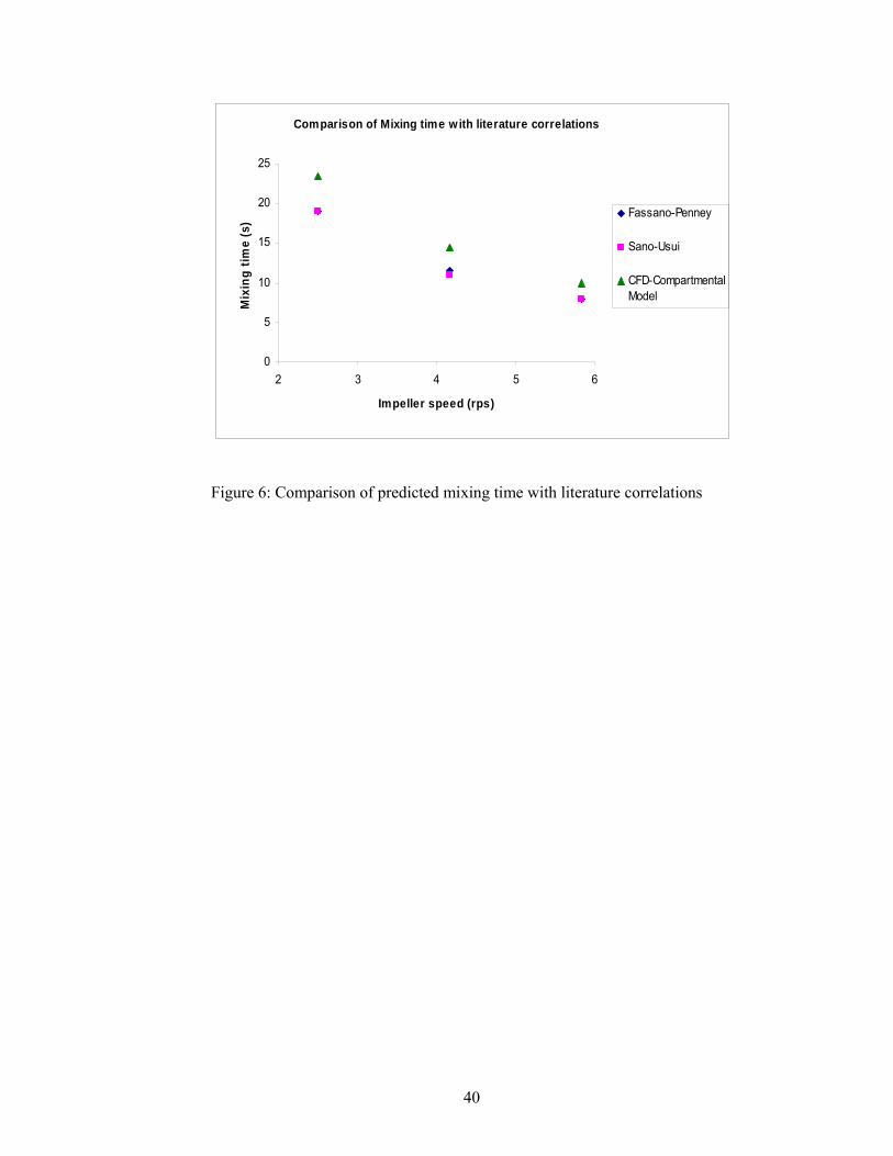
The mixing times predicted by the model at different impeller speeds
for 99% homogeneity (p=0.99) are compared with two correlations from the
literature. These correlations from Fasano and Penney (1994)22 and Sano and
Usui (1985)23 are respectively given by
5.017.2
06.1
)1ln(
⎟⎠⎞
⎜⎝⎛
⎟⎠⎞
⎜⎝⎛
−−=
HT
TDN
pt
imp
m ……………….. (24)
imp
b
m N
nTb
TD
t
47.051.080.1
8.3 −−−
⎟⎠⎞
⎜⎝⎛
⎟⎠⎞
⎜⎝⎛
= ……………….. (25)
The constants for equation (24) are valid for fully turbulent regime
(Reimp>10,000). At lower Reynolds Number the mixing time would be greater
than that predicted by this equation. For equation (25), all the measurements
were done for Reimp>5000 and the constants are valid only for 99%
homogeneity in the tank.
Comparison of the predicted mixing times at different impeller speeds
with the two correlations is shown in Figure 6. The model predictions
compared reasonably well with the correlation values to achieve 99%
homogeneity in mixing. Studies on mixing in stirred tank reactors also show
that in the completely turbulent regime, the dimensionless mixing time defined
as mimptN becomes constant when plotted against the impeller Reynolds
number. Such a plot based on the predicted mixing time in Figure 7 also
exhibits essentially a constant value. The average value of the dimensionless
mixing time as predicted by the model is about 59.
21
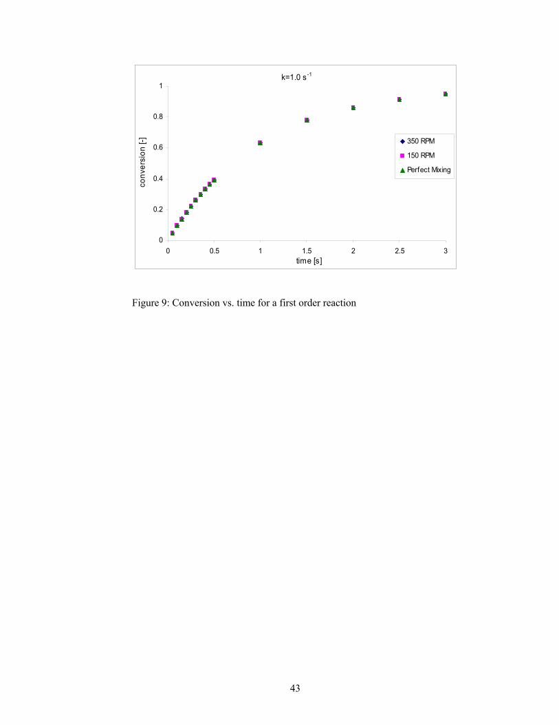
First and Second Order Kinetics:
In order to test the model developed, single reactions of first and second order
kinetics are studied at two different impeller speeds (150 and 350 RPM) for a
batch system. The reaction time scale is taken as 1 second. It has to be noted
that the inert mixing times at 150 and 350 RPM are around 19 seconds and 9
seconds, respectively, i.e. the reaction time scale is kept small compared to the
time scale of mixing. It is therefore expected that mixing should have an
influence on reactor performance under these conditions.
First Order Kinetics:
The reaction stoichiometry for this case is given by B Products. The
reactant B is added as a pulse to solvent A present in the reactor. The
concentration of the reactant B in the pulse is 100 mol/m3 , which would result
in a mean B concentration of 10 mol/ m3. The ratio of the added volume of
reactant B to the total liquid volume in the reactor is ~0.1. It is assumed that
the reactor volume and the flow field do not change significantly due to the
addition of reactant B. The number of compartments used for simulation is
594 (11×9×6: axial×radial×angular) at 150 RPM and 216 (6×6×6:
axial×radial×angular) at 350 RPM.
The difference in the mixing behavior of the system at different
impeller speeds is visible in Figure 8 which shows a plot of the dimensionless
standard deviation of the concentration of B in the reactor vs. conversion. The
conversion is calculated based on the volume averaged mean concentration of
the reactant in the reactor. The standard deviation is larger at lower impeller
speed, i.e. as expected mixing is poorer under this condition. On the other

22
hand, Figure 9 shows a comparison of the reactor performance at the two
speeds and that predicted by the classical perfectly mixed stirred tank model
(instantaneous mixing at all length scales). The plots can be seen to overlap
each other. This confirms the fact that conversion of a first order reaction is
always independent of the mixing behavior of the system.
Second Order Kinetics:
The reaction stoichiometry for this case is A+B Products, and the reaction
is first order in each reactant and is second order overall. The conditions are
the same as stated in the preceding section. The mean concentration of
reactant A already present in the reactor is 10 mol/ m3 so that the molar ratio of
the two reactants fed to the system is equal to 1.
As before, the difference in the mixing behavior at the two conditions
can be observed in Figure 10. However, now the reaction kinetics being non-
linear, mixing should have an influence on reactor performance. This is shown
in Figure 11. Since this is a batch process, the slower the mixing the larger is
the time needed to achieve a desired level of conversion (up to 90%
conversion is shown in the plot).
Effect of Mixing on Multiple Reactions:
Mixing effects on the performance of chemical reactors become much more
significant when there are multiple reactions taking place in the system with
widely varying time scales. The formation of the desired products can be
increased if mixing effects in such reactions can be predicted. From an

23
environmental point of view, this can lead to the minimization of waste
generation as well.
Paul and Treybal (1971)24 had performed experiments with a second
order, competitive-consecutive reaction scheme and showed the effect of feed
location and mixing for a homogeneous, multiple-reaction system. The
reaction used in that study was the iodination (B) of L-tyrosine (A) to produce
3-iodo-L-tyrosine (R) and 3,5-diiodo-L-tyrosine (S). The reaction scheme can
be written as
SBRRBA
k
k
⎯→⎯+
⎯→⎯+2
1
The component R is the desired product of the reaction. The kinetic constants
for the two reactions, as obtained from their study at 298K, are
1131 035.0 −−= smolmk and 113
2 0038.0 −−= smolmk . The first reaction is an
order of magnitude faster than the second reaction. These reactions are slow
enough to ignore micromixing effects (as shown later) and have been used
earlier to demonstrate the effect of macromixing using the Network of Zones
model25 as well.
The system comprises of semi-batch addition of reactant B (iodine)
into pre-charged A (L-tyrosine) which has an initial concentration
of 3200 −molm . The concentration of reactant B in the feed is 32000 −molm . The
feeding time for B is 15 seconds and the molar ratio of reactant A to the total
amount of B fed to the system is 1. The impeller speed is 1600 RPM. The
number of compartments used for simulation is 1560 (13×10×12:
axial×radial×angular). A schematic of the geometry used for the experimental
study is shown in Figure 12. Two feed lines were used for the addition of

24
reactant B, one at the top and the other below the impeller. The semi-batch
injection of B is modeled as a series of discretized feeds at small intervals of
time. The time interval between two feeds is taken as 0.5 seconds. No
significant difference is observed by decreasing the time interval further.
An estimate of the micromixing time scale can be obtained as26
εν24.17=microt ………………….. (26)
where ν is the kinematic viscosity and ε is the average kinetic energy
dissipation rate given by
153 −= Timp VDPoNε …………………. (27)
Assuming Po as 5 for a Rushton turbine operating in the completely turbulent
regime, the estimated micromixing time scale for the condition simulated turns
out to be ~0.007 s. The reaction time scale based on the fastest reaction can be
estimated as
01
1
Arxn Ck
t = ………………… (28)
which is ~0.143 s. Since the micromixing time scale is much smaller than the
time scale of the fastest reaction, performance will be limited by macromixing,
and micromixing effects can be neglected.
The effect of the feed location on the mixing behavior of the system is
shown in Figure 13. Mixing is poorer when the feeding is done from the top as
evidenced by a much higher standard deviation of concentration of B
compared to the bottom feed. Figure 14 shows the yield of R (defined as
0AR CC ) as a function of time. The yield is lower when the top feed-line is
25
used, thereby producing more of the undesired product S due to local over-
reaction.
In their experimental study, Paul and Treybal24 measured the yield of
the product R when the reaction reached completion. Figure 15 shows a
quantitative comparison of the measured yield of R and the yield predicted by
the compartmental model and the perfectly mixed model at the end of the
reaction for the two feed points. The conventional perfectly mixed model
would predict a yield of 75.5% when there is no mixing limitation24. The
compartmental model does a better job in predicting the product yield for
different feed locations. The agreement between the experimental result and
model prediction is reasonable, though the performance is slightly under-
predicted for the top feed-line. Under-predicting the yield of R implies that
mixing is under-predicted for that case (since poorer mixing produces less R).
One of the reasons for this could be the under-estimation of the exchange
coefficient term in the model equation. To check the sensitivity of the
predictions to this term, simulations were done by dropping the exchange
terms completely (retaining only the mean flow) and also by increasing the
exchange coefficients by a factor of 2. The results are shown in Figure 16. The
top-feeding turns out to be quite sensitive to the exchange term, while the
bottom one is almost independent of the exchange term. This is in line with
the discussion presented earlier.
Summary and Conclusions:
In this work, the CFD-based compartmental model is developed and employed
to predict the effect of mixing on the performance of stirred tank reactors. The

26
model has been shown to capture the essential features of macromixing in the
reactor. For reactive systems, a discretization scheme has been developed
based on the time scales of the system. The effect of the feed location on the
product yield and selectivity is also captured for multiple reaction system and
the results are in reasonable agreement with those experimentally observed.
Based on the results obtained it can be concluded that the dispersion term
(mesomixing) in the model equation is important when reactant feeding is far
from the impeller. When feeding is close to the impeller, convection
(macromixing) dominates and the contribution of the dispersion term is not
significant.
Acknowledgement
The support by the NSF-ERC award (EEC-0310689) from the National
Science Foundation is hereby greatly acknowledged by the Washington
University team. Additional support from Air Products and Chemicals Inc.
through CREL membership is appreciated. We also appreciate the useful
discussions and technical inputs from Carlos Valenzuela, Bernie Toseland and
Tony Cartolano of Air Products and Chemicals Inc.

27
Nomenclature:
A: Constant
b: Blade height (m)
C: Clearance of impeller from tank bottom (m)
cc: Concentration of component c (mol-m-3)
cc : Mean concentration of component c (mol-m-3)
'cc : Fluctuating concentration (mol-m-3)
⟩⟨ cc : Volume averaged concentration (mol-m-3)
⟩⟨ mcc , : Cup-mixing concentration (mol-m-3)
D: Impeller diameter (m)
Dm: Molecular diffusivity (m2-s-1)
Dt: Turbulent dispersion coefficient (m2-s-1)
H: Liquid height (m)
k: Turbulent kinetic energy (m2-s-2)
kex: Exchange coefficient (m-s-1)
le: Eddy length scale (m)
nb: Number of blades
N: Number of compartments
Nimp: Impeller speed (rps)
NR: Number of reactions
p: Degree of homogeneity, i.e. local concentrations do not vary more than
(1-p)% of the mean concentration
Q: Volumetric flow rate (m3-s-1)
S: Surface area (m2)
T: Tank diameter (m)

28
t: Time (s)
tm: Mixing time (s)
iu : Mean velocity (m-s-1)
'u : Fluctuating velocity (m-s-1)
⟩⟨ mu : Surface average velocity (m-s-1)
uax: Axial velocity (m-s-1)
urad: Radial velocity (m-s-1)
uθ: Circumferential velocity (m-s-1)
V: Compartment volume (m3)
VT: Total fluid volume (m3)
ε: Kinetic energy dissipation rate (m2-s-3)
σ: Concentration standard deviation (mol-m-3)
ν: Kinematic viscosity (m2-s-1)
Dimensionless Numbers:
Da: Damkohler Number
Pe: Peclet Number
Re: Reynolds Number
Sc: Schmidt Number
ScT: Turbulent Schmidt Number
Po: Power Number

29
Time Scales:
Reaction time scale: )(/ 00 CRC
Convection time scale: 0U
L
Mean Residence time: inQ
V
Dispersion / Mesomixing time scale: tD
L2

30
References:
1. Vicum, L., Ottiger, S., Mazzotti, M., Makowski, L. and Baldyga, J., Multi-
scale modeling of a reactive mixing process in a semibatch stirred tank,
Chemical Engineering Science, 2004; 59: 1767
2. David, R. and Villermaux, J., Interpretation of Micromixing Effects on fast
Consecutive-Competing Reactions in Semi-Batch Stirred Tanks by a Simple
Interaction Model, Chem. Eng. Commun., 1987; 54: 333
3. Baldyga, J. and Bourne, J.R., A Fluid Mechanical Approach to Turbulent
Mixing and Chemical Reaction: II; Micromixing in the light of Turbulence
Theory, Chem. Eng. Commun., 1984a ; 28: 243
4. Madras, G. and McCoy, B.J., Kinetics and reactive mixing: Fragmentation
and coalescence in turbulent fluids, AIChE J., 2004; 50, 4: 835
5. Mann, R. and Hackett, L.A., Fundamentals of Gas liquid mixing in a stirred
vessel: An analysis using network of back-mixed zones, 6th European
Conference on Mixing, 1988
6. Holden, P.J. and Mann, R., Turbulent 3-D mixing in a stirred vessel:
Correlation of a Networks-of-Zones image reconstruction approach with
pointwise measurements, IChemE Symposium Series, 1996; 140: 167
7. Boltersdorf, U., Deerberg, G. and Schluter, S., Computational studies of the
effects of process parameters on the product distribution for mixing sensitive
reactions and on distribution of gas in stirred tank reactors, Recent Res.
Devel. Chemical Engg., 2000; 4: 15
8. Rahimi, M., Senior, P.R. and Mann, R., Visual 3-D modeling of stirred
vessel mixing for an inclined blade impeller, Trans IChemE, 2000; 78, Part A:
348

31
9. Rahimi, M. and Mann, R., Macro-mixing, partial segregation and 3-D
selectivity fields inside a semi-batch stirred reactor, Chemical Engineering
Science, 2001; 56: 763
10. Smith III, F.G., A model of transient mixing in a stirred tank, Chemical
Engineering Science, 1997; 52, 9: 1459
11. Brucato, A., Ciofalo, M., Grisafi, F. and Tocco, R., On the simulation of
stirred tank reactors via computational fluid dynamics, Chemical Engineering
Science, 2000; 55: 291
12. Bujalski, J.M., Jaworski, Z., Bujalski, W. and Nienow, A.W., The
influence of the addition position of a tracer on CFD simulated mixing times
in a vessel agitated by a Rushton turbine, Trans IChemE, 2002; 80, Part A:
824
13. Alexopoulos, A.H., Maggioris, D. and Kiparissides, C., CFD analysis of
turbulence non-homogeneity in mixing vessels: A two-compartment model,
Chemical Engineering Science, 2002; 57: 1735
14. Bezzo, F., Macchietto, S. and Pantelides, C.C., General hybrid
multizonal/CFD approach for bioreactor modeling, AIChE J., 2003; 49, 8:
2133
15. Akiti, O. and Armenante, P.M., Experimentally-validated micromixing-
based CFD model for fed-batch stirred tank reactors, AIChE J., 2004; 50, 3:
566
16. Rigopoulos, S. and Jones, A., A hybrid CFD-reaction engineering
framework for multiphase reactor modeling: basic concept and application to
bubble column reactors, Chemical Engineering Science, 2003; 58: 3077

32
17. Bird, R.B., Stewart, W.E. and Lightfoot, E.N., Transport Phenomena,
John Wiley and Sons, 1994
18. Fox, R.O., Computational methods for turbulent reacting flows in the
chemical process industry, Revue De L’ Institut Francais Du Petrole, 1996;
51, 2: 215
19. Baldyga, J., Turbulent mixer model with application to homogeneous
instantaneous chemical reactions, Chemical Engineering Science, 1989; 44, 5:
1175
20. Fox, R.O., Computational models for turbulent reacting flows, Cambridge
University Press, 2003
21. Ranade, V.V., Computational Flow Modeling for Chemical Reactor
Engineering, Academic Press, 2002
22. Fasano, J.B., Bakker, A. and Penney, W.R., Advanced Impeller Geometry
Boosts Liquid Agitation, Chemical Engineering, Aug 1994
23. Sano, Y. and Usui, H.., Interrelations among mixing time, power number
and discharge flow rate number in baffled mixing vessels, Journal of Chem
Engg of Japan, 1985; 18: 47
24. Paul, E.L. and Treybal, R.E., Mixing and product distribution for a liquid-
phase, second-order, competitive-consecutive reaction, AIChE J., 1971, 17, 3:
718
25. Mann, R. and El-Hamouz, A.M., Effect of macromixing on a
competitive/consecutive reaction in a semi-batch stirred vessel, Proc. Euro.
Conf. on Mixing, 1991

33
26. Assirelli, M., Bujalski, W., Eaglesham, A. and Nienow, A.W., Study of
micromixing in a stirred tank using a Rushton turbine: Comparison of feed
positions and other mixing devices, Trans IChemE, 2002; 80, Part A: 855

34
List of Figure Captions:
Figure 1: Configuration of a single backmixed compartment showing
neighboring interconnected compartments
Figure 2: A discretized compartment in the compartmental framework
Figure 3: Discretization in the axial direction
Figure 4: Schematic diagram of the geometry used
Figure 5: Convergence of predicted mixing time with number of
compartments
Figure 6: Comparison of predicted mixing time with literature correlations
Figure 7: Dimensionless mixing time (predicted) vs. Reynolds Number
Figure 8: Dimensionless standard deviation vs. conversion for a first order
reaction
Figure 9: Conversion vs. time for a first order reaction
Figure 10: Dimensionless standard deviation vs. conversion for a second order
reaction
Figure 11: Conversion vs. time for a second order reaction
Figure 12: Details of the geometry used for the simulation of multiple
reactions (Paul and Treybal, 1971)
Figure 13: Dimensionless standard deviation vs. time for a semi-batch second
order, competitive-consecutive reaction scheme
Figure 14: Yield of R as a function of time for the multiple reaction scheme
Figure 15: Comparison between measured and predicted yield of R at the end
of the reaction for the two feed locations
Figure 16: Sensitivity of the exchange term on the prediction of yield

35
Figure 1: Configuration of a single backmixed compartment showing
neighboring interconnected compartments

36
Figure 2: A discretized compartment in the compartmental framework
xθ
xz

37
Figure 3: Discretization in the axial direction

38
Figure 4: Schematic diagram of the geometry used

39
0
5
10
15
20
25
30
35
0 100 200 300 400 500 600 700 800
Number of compartments
Mix
ing
time
(s)
150 RPM
250 RPM
350 RPM
Figure 5: Convergence of predicted mixing time with number of
compartments
40
Comparison of Mixing time with literature correlations
0
5
10
15
20
25
2 3 4 5 6
Impeller speed (rps)
Mix
ing
time
(s)
Fassano-Penney
Sano-Usui
CFD-CompartmentalModel
Figure 6: Comparison of predicted mixing time with literature correlations

41
20.0
30.0
40.0
50.0
60.0
70.0
10000 12000 14000 16000 18000 20000 22000 24000 26000 28000
Re
Nim
ptm
Figure 7: Dimensionless mixing time (predicted) vs. Reynolds Number

42
k=1.0 s-1
0
0.5
1
1.5
2
2.5
3
3.5
0 0.2 0.4 0.6 0.8 1conversion [-]
σ / C
B [-
]
350 RPM
150 RPM
Figure 8: Dimensionless standard deviation vs. conversion for a first order
reaction
43
k=1.0 s-1
0
0.2
0.4
0.6
0.8
1
0 0.5 1 1.5 2 2.5 3time [s]
conv
ersi
on [-
] 350 RPM
150 RPM
Perfect Mixing
Figure 9: Conversion vs. time for a first order reaction

44
kCa0=1.0 s-1
0
0.5
1
1.5
2
2.5
3
3.5
0 0.1 0.2 0.3 0.4 0.5 0.6 0.7 0.8 0.9 1conversion [-]
σ / C
B [-
]
350 RPM
150 RPM
Figure 10: Dimensionless standard deviation vs. conversion for a second order
reaction

45
kCa0=1.0 s-1
0
0.2
0.4
0.6
0.8
1
0 2 4 6 8 10 12 14time [s]
conv
ersi
on [-
]
150 RPM
350 RPM
Perfect Mixing
Figure 11: Conversion vs. time for a second order reaction

46
Figure 12: Details of the geometry used for the simulation of multiple
reactions (Paul and Treybal, 1971)

47
0
1
2
3
4
0 5 10 15 20time [s]
σ / C
B [-
]
top [1]
bottom [2]
Figure 13: Dimensionless standard deviation vs. time for a semi-batch second
order, competitive-consecutive reaction scheme

48
0
0.2
0.4
0.6
0.8
0 5 10 15 20time [s]
CR
/ C
A0 [-
]
top [1]
bottom [2]
Figure 14: Yield of R as a function of time for the multiple reaction scheme

49
0
10
20
30
40
50
60
70
80
Yiel
d of
Des
ired
Prod
uct [
%]
Top Bottom
Feed Locations
Experiment (Paul &Treybal,1971)
Compartmental Model
Perfect Mixing Assumption
Figure 15: Comparison between measured and predicted yield of R at the end
of the reaction for the two feed locations

50
0
10
20
30
40
50
60
70
80
Yie
ld o
f R [%
]
Top Bottom
Model (f=0)
Model (f=1)
Model (f=2)
Experiment
Figure 16: Sensitivity of the exchange term on the prediction of yield ( f
denotes the multiplication factor to the normal exchange coefficients obtained
earlier, i.e. f=0 signifies no exchange term is used)