ceve 310/510 principles of environmental engineering

Changha Lee

School of Chemical and Biological Engineering

Seoul National University

http://artlab.re.kr

고도산화환원환경공학연구실

Advanced Redox Technology (ART) Lab

Water Pollution-4-Surface Water Quality

Sources Sinks

Atm. Reaeration Discharge (BOD) respiration

Photosynthesis Nitrification

Advection (confluence) Benthal O2 demand (sediments)

Oxygen Depletion in Rivers

• River health is directly related to DO concentration profile.

• The critical level for DO is ~3 mg/L.

• No fish will survive if DO < 1 mg/L.

• Lower DO: floating sludge, odors and fungal growth

• Factors Affecting DO profile:

• Temperature also a factor (less DO at high T)

√ Oxygen Depletion in Rivers

DO Sag Curve and Aquatic Wildlife

√ Consider a waste discharge mixing with a stream flow

DO Model: Discharge and Mixing

BOD of mixed stream (x = 0)w w r ro

w r

Q L Q LL

Q Q

+= =

+

• Initial DO deficit (D0) in combined flow is the saturation value

minus the actual DO.

rw

rrww

satQQ

DOQDOQDOD

+

+−=

)()(0

Do not confuse DO with D0

DO Model: Discharge and Mixing

√ O2 depletion is primarily due to heterotrophic respiration.

• Deoxygenation can occur rapidly and results in an oxygen deficit (relative to

typical levels)

• Deoxygenation rate (proportional to BOD) = kdLt = kdL0exp(-kdt)

kd = deoxygenation rate coefficient ( k)

Lo = ultimate carbonaceous biochemical O2 demand

DO Model: Deoxygenation

O

tt

ktt

dLkL

dt

L L e−

=

=

k = kd

Recall the BOD degradation rate

= dD/dt

• River was characterized as BOD = 7 mg/L, flow = 6 m3/s.

Discharge into the river at City A: BOD = 40 mg/L, inflow = 1 m3/s.

What is the BOD just after discharge and at city B, 20 hours after discharge

at City A? (kd = 0.15 d-1)

Qm = total flow = 7 m3/s

Lo = (6 m3/s)(7 mg/L) + (1 m3/s)(40 mg/L)

7 m3/s

Lo= 11.7 mg/L just downstream

At City B, L = 11.7 e -0.15 (20/24) = 10.3 mg/L

Example

City A

City B(20 h away from City A)

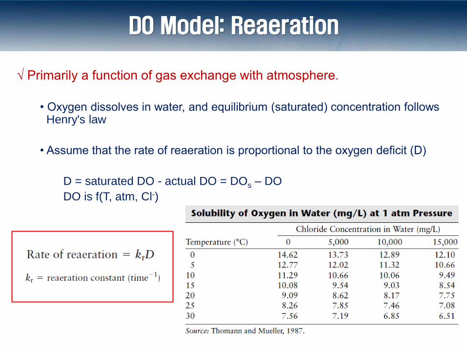
√ Primarily a function of gas exchange with atmosphere.

• Oxygen dissolves in water, and equilibrium (saturated) concentration followsHenry's law

• Assume that the rate of reaeration is proportional to the oxygen deficit (D)

D = saturated DO - actual DO = DOs – DO

DO is f(T, atm, Cl-)

DO Model: Reaeration

• Reaeration rate = krD

- Where kr = reaeration coefficient (depends on mixing and flow rate)

0.1 to 0.23/day for small pounds

0.69 to 1.5/day for swift streams

• Generally slower than DO consumption (i.e., deoxygenation) when the BOD is high

(e.g., near the discharge point).

kr =3.9 u

H32

kr – reaeration rate (1/day)

u – average stream velocity (m/s)

H – average stream depth (m)

DO Model: Reaeration

√ The combination of the deoxygenation and reaeration rates represent

the O2 behavior.

• Assumptions

- Mixing occurs across the river cross-section y and z

- No mixing in x direction (no dispersion in flow direction)

- Point source, plug flow conditions:

Solution to plug flow is the first order expression

DO Model: Deoxygenation & Reaeration

• Rate of increase of oxygen deficit = rate of deoxygenation – rate of reaeration

• Solution:

dk t

d o r

dDk L e k D

dt

−= −

Do : initial DO deficit of river-sewage mixture

tk-o

tk-tk-

dr

od rrd e D + )e - (ek-k

Lk = D

Streeter-Phelps Oxygen Sag Equation

• Quantify Deficit (in dissolved oxygen) progressing downstream (in terms of time

or distance)

• Distance is easier to conceptualize and can be easily substituted

Distance = (velocity) x (time)

x = u x t

x/uk-

o

/xk-/xk-

dr

0d rrd e D + )e - (ek-k

Lk = D

uu

Streeter-Phelps Equation

Deoxygenation > reaeration

Deoxygenation = reaeration

Deoxygenation < reaeration


• Deoxygenation > reaeration at the beginning

• At some point the rates are equal – this is when DO is a minimum

(determined by setting dD/dt = 0)

Critical point,

• Later, deoxygenation rate decreases (with BOD) and reaeration becomes faster.

tc =1

kr − kdlnkr

kd1−Do kr − kd( )kdLo

dD

dt= kdLoe

−kt − krD


DO Sag Curve and BOD Profile

• Where will the critical point occur if

Lo= BOD of river/sewage mix = 10.9 mg/L

DO at mix. point = 7.6 mg/L

u = 0.3 m/s, depth = 3.0 m

T = 20 °C, kd = 0.2 /day

Example

tc =1

kr − kdlnkr

kd1−Do kr − kd( )kdLo

For kr use the O’Connor-Dobbins empirical formula

To find the critical point

with the given flow rate and stream size

x = u t = 0.3 m/s * 3600*24*2.67 days

= 69,300 m

1/2

3 3/2 1.52

3.9 3.9 u 3.9 0.3 = = 0.41/day

H 3r

uk

H

= =

( )1ln 1

1 0.41 1.5(0.41 - 0.2) = ln 1 - = 2.67 days

0.41 - 0.2 0.2 0.2 10.9

o r drc

r d d d o

D k kkt

k k k k L

−= − −

Example (Solution)

First, we need to find kr and Do

Do = DOs (from the table) – DO = 9.1 − 7.6 mg/L = 1.5 mg/L

• What will be the minimum DO in this river? Could find the minimum DO value

tc = 2.67 days

Using the oxygen sag equation with this value of t,

we find that the maximum oxygen deficit is 3.1 mg/L.

If the deficit is 3.1 mg/L and DO saturation is 9.1 mg/L

DOmin = 9.1 − 3.1 = 6.0 mg/L

Example

tk-o

tk-tk-

dr

od rrd e D + )e - (ek-k

Lk = D

• The model can be used to determine the assimilative capacity of rivers, or to set

permits for sewage discharge.

−If the proposed discharge results in DO that is too low, allowed sewage is

should be reduced (lower BOD concentration and/or inflow rate).

• Temperature effects are important - in hot weather the DOsat is lower and

respiration is faster.

• More complex models consider photosynthesis and diurnal variations (sine

functions). Other factors such as benthal DO demand by sludge and

nitrification can also be considered.

(http://en.wikipedia.org/wiki/Streeter-Phelps_equation#Expanded_model)

Remarks

Water Quality of Lakes & Reservoirs

• Lakes and Reservoirs require special attention because they are not moving

or flowing (no easy flushing) so inputs and oxygenations process have

different effects

• Oligotrophic

− A new body of water (young lake)

− “little nutrients”

• Eutrophic

− “well fed”

− Phytoplankton grow and die (drop to the bottom)

− Organic matter decays, using up oxygen

− Silt and organic matter accumulate at bottom

→ lake becomes more shallow and warms up

→ also becomes murky

→ eventually becomes a marsh or a bog

• Eutrophication: natural aging process takes thousands of years.

How Do Humans Affect Eutrophication?

• Generation of:

− municipal wastewater

− industrial wastes

− agricultural runoff

• Accelerated eutrophication due to human

activities

= cultural eutrophication

All these inputs

stimulate algae growth

How Do Humans Affect Eutrophication

• Algae blooms

− Odor & taste problems

− Algal toxins (e.g., microcystin)

− DO consumed with algal decay

• Low dissolved oxygen may drive out fish

• Anaerobic conditions – odor (H2S), dissolution of heavy metals

pH drop due to fatty acids

√ Result of eutrophication:

Eutrophication Factors

• Sunlight affects photosynthesis (algae need light).

• Oligotrophic lakes (e.g.,. Lake Tahoe)

− Clear and photosynthesis occurs down to 100 m +

• Eutrophic lakes

− Murky and photosynthesis may be limited to upper layer.

√ Sunlight

• Layers based on photosynthesis activity

− Euphotic Zone:

O2 input by photosynthesis

> O2 removed by respiration

− Aphotic Zone:

little light (little photosynthesis,

mainly benthic activity)

• Many nutrients are important to life

− C, N, P, S, Ca, Mg, K, Se, Pb, Zn, Cu….

− To control algae growth we can control nutrient levels,

but which one(s)?

phosphorus (P) or nitrogen (N)

• Liebig’s Law of the Minimum –

– Total biomass of any organism is determined

by the nutrient present in the lowest concentration

relative to the organism’s stoichiometric requirement

(which is determined by the organism’s elemental

composition)

√ Nutrient


• If you determine which is the limiting nutrient and make it scarcer, the algae

population will be reduced.

• Eutrophic lakes have primarily blue-green algae (cyanobacteria), which can

get N from the atmosphere

− Need to focus on limiting P

0.01 mg/L-P “acceptable”

0.02 mg/L-P “excessive” → cause algal blooms

• Very deep lakes

− Less recirculation of P, tend to be oligotrophic.


√ Nutrient

• Consider empirical elemental composition of algae:

– C106H263O110N16P

• N/P = 16 (14 g/mol) / 1 (31 g/mol) = 7.2

– For every 7.2 g of N utilized, 1 g of P is used

• Rule of thumb:

N/P > 10 → P is limiting

N/P < 5 → N is limiting

• No algae blooms will occur if:

– P < 0.015 mg/L

– N < 0.3 mg/L


√ Nutrient

S = rate of P addition from all point-source(s) (g/s)

Q = inflow/outflow rate from lake (m3/s)

Vs = P settling rate (m/s)

A = surface area of lake (m2)

C = concentration of phosphorus (g/m3)

in

s

QC SC

Q v A

+=

+

• For well mixed lakes at steady state, small S, and Qin = Qout, sink term is

mainly due to settling

Rate of P addition = Rate of P removal

QCin + S = QC + vSAC


√ Phosphorus

• Temperature affects water density.

− Water has a maximum density at 4 degrees C

• Density ↓ for T < 4℃

• Density ↓ for T > 4℃


√ Temperature

• In the summer:

– Water is warmed by the sun > 4℃

– Top layer warms up, becomes less dense than bottom layer

→ Top warmer layer stays at the top of the lake

• In the winter:

– Top water is colder than 4℃

– As top layer cools, it becomes less dense than bottom layer

→ Top layer (ice) stays at top of the lake

• In both extremes, there is little vertical mixing due to temperature related

density differences – this is known as thermal stratification

Thermal Stratification

• To get from summer temperature profile to the winter temperature profile

(and vice versa), top layer must pass through a point when the

temperature is 4℃ (denser, sinks and displaces bottom layer water which

rises)

• This allows for periodic mixing (and nutrient recycling) in climates where it

gets cold enough to freeze and/or warm enough to thaw.

• Due to thermal stratification, the warm and cold parts of the lake act

independently


• Epilimnion – (usually) upper warmer layer, uniform T, mixing is affected by

waves and wind

• Hypolimnion – cold, lower layer

• Transition happens in the thermocline/metalimnion

• For both eutrophic and oligotrophic lakes, warm upper layer (epilimnion) can

get oxygen from reaeration and photosynthesis

• In the hypolimnion, DO only from photosynthesis, this may happen in a

oligotrophic lake but unlikely in a eutrophic (turbid) lake

√ How does this stratification affect DO?


Acidification

• Rainwater in equilibrium with CO2 has a pH of 5.5

• Northeastern US rain can have a pH < 4

• California fogs have pH around 3

• Low pH values primarily due to S and N oxide emissions

(generate sulfuric and nitric acid)

• The term acid deposition includes both acid rain and the deposition

of acid gases and particles

• Acid deposition effects

– Materials : attacks marble, limestone as well as metals

– Terrestrial ecosystems : stresses plants, hinders growth

– Aquatic ecosystems : fish & aquatic life

Acid Rain

• Lakes (fish)

• Soil (agriculture)

• Art

Acid Rain and Lakes

• If the pH of a lake falls below 5.5, aquatic life becomes stressed.

• Few species will survive in a pH below 5.

• Some lakes have natural buffers or chemicals to neutralize the H+

• Carbonates are important buffers: H2CO3 ↔ H+ + HCO3-

• As H+ is added to the aquatic system, carbonic acid is formed and

pH does not change if there is an infinite source of bicarbonate (buffering).

• There is a documented correlation between the pH and the fish population

– Bicarbonate lakes are well populated.

– Many acidic lakes are barren.

Acid Rain and Lakes

• Bicarbonate buffering strongly resists acidification until pH drops below 6.3.

As more H+ ions are added, pH decreases rapidly after the point.

Acid Rain and Lakes

• What determines the bicarbonate concentration and vulnerability to acidification?

– Soils, size of water body, vegetation and geography

• Soils are important because they are the source of limestone for buffering; lakes

with calcareous soils (lots of limestone) are well neutralized

• Soils of nearby land are also important

– If soils are thin and impermeable, the runoff will enter the water

body with little contact between the precipitation and natural buffers

• Local vegetation can also affect acidification

– Deciduous trees (loose leaves annually) tend to decrease acidity

– Conifers (pine trees) tend to increase it

Acid Rain and Lakes

• Acidification also has effects on heavy metal mobility.

– Metals dissolve as the pH drops

e.g., Gibbsite

Al(OH)3 + 3 H+ ↔ Al3+ + 3H2O

• Aluminum is toxic to fish, and even if the pH doesn't kill them

the aluminum could.

– Air pollution control is mitigating acid rain

ceve 310/510 principles of environmental engineering

Documents