central simple algebras - biuu.math.biu.ac.il/~vishne/publications/doct.pdf · central simple...
TRANSCRIPT
Central Simple Algebras
Uzi Vishne
Department of Mathematics
Ph.D. Thesis
Submitted to the Senate of Bar-Ilan University
Ramat-Gan, Israel Jul. 2000

This work was carried under the supervision of Prof. Louis H. Rowen(Department of Mathematics), Bar-Ilan University.


Dedicated to my wife Tali,and to Gal, Ariel, Hadar and Rotem,who didn’t help much with the mathematics,but are invaluable in any other aspect.
I deeply thank Professor L. Rowen for being a truly great teacher.His support and guidance go way beyond the scope of this work.

Contents
Preface i
Chapter 1. p-Algebras 11. Field Extensions in Characteristic p 21.1. Inseparable Extensions 21.2. Cyclic Separable Extensions 31.3. Composite Extensions 51.4. Relative H groups 71.5. Counting Cyclic Extensions 121.6. Going Up One Stage 152. Cyclic p-Algebras 183. Presentation for pBr(F ) 213.1. The Merkurjev-Suslin Theorem 213.2. Generators and Relations for pBr(F ) 224. Generators of p-Algebras 264.1. Generators of Cyclic p-Algebras 264.2. The Connection Theorem 294.3. Generators of Products of Symbols 304.4. Quaternions in Characteristic 2 325. Generators of pBr(K) 335.1. The Subgroup [K,F 345.2. The Trace Map 365.3. Quaternions over C2-fields of Characteristic 2 375.4. Two Types of Symbols 386. Hilbert’s Theorem 90 for pBr(K) 396.1. Hilbert’s Theorem 90 in the Prime-to-p Case 406.2. Elementary Results 416.3. A Quantitative Theory 446.4. Hilbert’s Theorem 90 for pBr(K) 476.5. The Invariant Subgroup pBr(K)σ 526.6. Remarks on Corestriction 56
Chapter 2. Brauer Algebras 591. Introduction 59
1
2. The Leading Monomial Technique 593. The Generic Elements Construction 614. Brauer’s Example 625. Property D(p) for Algebras of Degree p2 666. Brauer’s Example in Degree n = p3 67
Chapter 3. Dihedral Crossed Products With Involution 711. Introduction 712. Involutions 723. Dihedral Crossed Products 76
Bibliography 79

Preface
Pick a finite dimensional algebra over a field F . Compute its (Ja-cobson) radical, and factor it out. What you get is a direct sum ofideals, each one a simple algebra. Each of these components is a fullmatrix ring over a division algebra, finite dimensional over F .
Finite dimensional division algebras are the building blocks of ringtheory. Make a list of all the possible division rings, learn how to liftproperties back from the semiprimitive case to the general case, andyou can study Artinian rings in general.
Emerging from the general structure theory of rings, the study ofdivision algebras started from isolated constructions (like that of thecyclic algebras by Dickson), and expanded during the thirties and for-ties to results like the structure theory of p-algebras, the description ofdivision algebras of low degree (both by A. Albert), the connection tocohomology (E. Noether), and the Albert-Brauer-Hasse-Noether theo-rem, which had great influence on the development of field arithmetic.
The vivid activity nowadays studies division algebras in their ownright, counting on the machinery of generic matrices, the connections toK-theory or field arithmetic, homology or algebraic geometry. There isa counter play between division algebras and many current branches ofmathematics, such as involutions and quadratic forms, Galois theory,local fields, Azumaya algebras, field arithmetic and number theory, andmany others.
If A is a simple algebra with center F , then F is a field, and we saythat A is central over F . Let K/F be a field extension, then A⊗FK iscentral simple over K.
Suppose A/F is finite, then we have the equality of dimensions[A⊗FK :K] = [K :F ]. By Wedderburn’s structure theorem, A =Mm(D) where D is a central division algebra over F . Let K = F ,the algebraic closure of F . Since there are no non-trivial finite dimen-sional division algebras over F , A⊗FF is a matrix algebra over F , sayA⊗FF =Mn(F ). It follows that the dimension [A :F ] = [A⊗FF :F ] =
n2. The degree of A is defined by deg(A) =√[A :F ]. The index of
A is the degree of the underlying division algebra, ind(A) = deg(D).
i

ii
The best way to hold all the information on finite central simplealgebras over F in one object is by means of the the Brauer group.Identify two algebras if they have the same underlying division algebra,and define multiplication by [A][B] = [A⊗FB]. The Brauer groupBr(F ) is the set of all classes [A] for A finite-dimensional central simpleover F . Inversion of elements is by [A]−1 = [Aop] (where Aop is thealgebra with the same additive structure and reversed multiplication;then A⊗Aop =M[A:F ](F )). Moreover, by means of the so-called Brauer
factor sets it can be shown that A⊗F ind(A) is a matrix algebra, so thatBr(F ) is a torsion group.
Suppose A is a division algebra. If B ⊆ A in an F -subalgebra,then CA(CA(B)) = B, and [B :F ] · [CA(B) :F ] = [A :F ]. As a result,the dimension of every subfield of A/F is bounded by the degree of A.Every subfield of A/F is contained in a maximal subfield, which hasdimension deg(A) over F . L/F of dimension n splits A (i.e. A⊗L ismatrices over L) iff L is a maximal subfield in an algebra B, similar toA in the Brauer group, with deg(B) = n [1, p. 60].
A is called a p-algebra if the underlying base field is of characteristicp, and the dimension of A over its center is a power of p. The basicstructure theorems of p-algebras were discovered around 1940, mostlyby Albert [1] and Jacobson, whereas in the harder case of prime-to-pdegree the progress was much slower. The breakthrough came around1980, with theorems of Amitsur (the construction of noncrossed prod-ucts) and Merkurjev-Suslin (connecting the Brauer group to algebraicK-theory), with the use of geometric methods that was possible mainlyin characteristic 0. While there was a lot of activity in the theory ofAzumaya algebras over commutative rings in characteristic p (e.g. Salt-man’s thesis [36] or [18]), certain aspects in the study of the p-part ofthe Brauer group itself seem to have been left behind.
Undoubtedly, the main method in the study of central simple alge-bras is by means of their subfields.
Our contribution in this work is in several directions. The mainsubject in Chapter 1 is the p-part of the Brauer group of fields withcharacteristic p. We begin with field extensions of p-power dimensionin characteristic p, starting from well-known facts, and going deeperinto classifying and counting composite extensions, thus producing anew proof for Witt’s theorem that the p-part of the absolute Galoisgroup of F is a free pro-p group, for the finitely generated case. Wethen discuss standard couples of generators of cyclic algebras of degreep, and give a description by generators and relations for the exponent-ppart of the Brauer group. In Section 4 we study various presentations
iii
of a given cyclic algebra of degree p, and show that an isomorphism oftwo cyclic p-algebras of degree p becomes tame (in the sense definedthere) if we tensor by Mp(F )
⊗2(p−2). In Section 5 we show that if K/Fis a finite separable extension, then the p-part of the Brauer group ofK is generated by the classes of symbol algebras of the form [a, β),where a ∈ K and β ∈ F . Moreover, [K :F ] + 1 symbols of this formare enough to express any symbol algebra of degree p over K. In thesixth section we study Hilbert’s theorem 90 in a general context, anddevelop some elementary tools which apply to any Abelian group ofexponent p equipped with an action of a cyclic group. Given any cyclicextension K/F , with arbitrary characteristic, these tools enable us tosuggest two interesting filtrations of subgroups of pBr(K), and studytheir connections. Special attention is given to the case charF = p. Weshow that under very mild assumption, Hilbert’s theorem 90 fails for
pBr(K). In Subsection 6.5 we study the invariant subgroup of pBr(K),and discuss some generic examples. Some easy results on corestrictionof cyclic algebras down odd dimension extensions are given in the lastsubsection, and used to give a counterexample to Hilbert’s theorem 90for groups of the form nBr(K).
In Chapter 2 we closely study a class of cyclic algebras, suggestedby Brauer as examples with arbitrary degree and exponent. We give aprecise formulation for the technique of passing to the leading mono-mial, and discuss some suggested construction of a noncrossed productof exponent p (a problem which is still open).
The last Chapter discusses algebras with involution. We study thepresentations of involutions in crossed products, and show that givenenough roots of unity, a dihedral crossed product with involution hasan Abelian maximal subfield.


CHAPTER 1
p-Algebras
Central simple algebras of degree a power of p over a field of char-acteristic p, are called p-algebras.
The theory of (finite-dimensional) central simple algebras naturallysplit into two parts. While the basic structure theory of p-algebras wasderived, mainly by Albert, back in the 40s, the theory of algebras withprime to p index still contains some very difficult open questions. Onthe other hand, some deep theorems from the 80s, most notably theMerkurjev-Suslin theorem, hold only for characteristic not dividing theindex (and in the presence of enough roots of unity).
The main theme of this chapter is to introduce some of the recentresults on prime-to-p index to the theory of p-algebras.
In the first section we describe the well-known Galois theory in char-acteristic p, and continue to study composite extensions, with resultson the number of subgroups of various types of the absolute Galoisgroup. The construction and basic properties of p-algebras of degree pare given in section 2.
In the third section we give a presentation of pBr(F ) by genera-tors (p-symbols) and relations. In the fourth section we define tameisomorphisms between cyclic p-algebras of degree p, following simi-lar ideas from the theory of the automorphism groups of polynomialrings. This is generalized to tensor product of cyclics of degree p, andthe main question is, given [a, b)∼=[a′, b′), what is the minimal m suchthat [a, b)⊗Mp(F )
⊗m∼=[a′, b′)⊗Mp(F )⊗m is tame. We show that the
m ≤ 2(p− 2) is always enough. Some special results for the case p = 2are also given.
In section 5 we show that if K/F is separable, then every p-symbolover K can be expressed as a sum of no more than [K :F ] + 1 symbolsof the form [a, β, where a ∈ K and β ∈ F . This is used to define atrace map on pBr(K) if K/F is Galois. Applications to the case of C2
fields of characteristic 2 are also given.Let K/F be a cyclic extension of fields. In section 6 we study to
what extent does Hilbert’s theorem 90 fail for the group pBr(K). Wedevelop some elementary but useful tools, and use them to show that
1
2 1. p-ALGEBRAS
Hilbert’s theorem 90 holds iff every invariant algebra of exponent p isthe restriction from F of an algebra of the same exponent. If bothstatements fail, we can match the two failures in the sense explainthere. We show that if [K :F ] is divisible by p, then under very weakassumptions Hilbert’s theorem 90 does fail for pBr(K). Elements ofthe invariant subgroup of pBr(K) are studied in the subsection 6.5, andproperties of the corestriction are used in the last subsection to showthat Hilbert’s theorem 90 does fail in some cases.
1. Field Extensions in Characteristic p
Let F be a field with charF = p > 0. In this section we brieflydescribe the (well known) theory of field extensions of such fields, ofdimension an exponent of p. In subsections 1.3 and 1.4 we study com-posite extensions, and use the results in subsections 1.5–1.6 to countextensions of various types, and bound the number of correspondingsubgroups in the absolute Galois group. The results can be used to givea new proof of Witt’s theorem that the p-part of the absolute Galoisgroup of F is a free pro-p group.
In subsequent sections we only use the basic facts from the first twosubsections, and the properties of HK/F defined in the third.
1.1. Inseparable Extensions. In every finite dimensional exten-sion L/F , there is an intermediate subfield F ⊆ K ⊆ L such that K/Fis separable, and L/K is purely inseparable. [L :K] is a power of p.
Lemma 1.1. Let b ∈ F . g(λ) = λp − b is either irreducible over F ,or splits in F .
Proof. Let y be a root of g in a splitting field, g1 the minimalpolynomial over F , and d = deg(g1).
g(λ) = λp − yp = (λ− y)p, and since g1 divides g (in F [y][λ]), it isa power of (λ− y). Then yd ∈ F as the constant coefficient of g1.
If d = p we are done. Otherwise, write αd + βp = 1, then y =(yd)αbβ ∈ F .
Corollary 1.2. F [λ]/⟨λp − b⟩ is either a field or a local ring ofdimension p over its residue field.
Every inseparable extension of dimension p of F is constructed inthis way: let S/F be such an extension, then some y ∈ S satisfiesyp ∈ F , y ∈ F , so that λp− b is the minimal polynomial of y. Then welet S = F [ p
√b].

1. FIELD EXTENSIONS IN CHARACTERISTIC p 3
If b1, b2 belong to the same class in F ∗/(F ∗)p , then obviouslyF [ p
√b1]∼=F [ p
√b2] . For a complete classification we need to introduce a
certain subfield of F .
The p-power map F → F , defined by x 7→ xp, is a homomorphismof fields (and thus monic). The image is denoted by F p = xp : x ∈ F,so that F∼=F p.
For example, suppose b1, b2 ∈ F , and denote Si = F [y : yp = bi].Then S1
∼=S2 iff F p[b1]∼=F p[b2], since Spi = F p[bi].
The exponent of a purely inseparable extension S/F is the leastq (a power of p), for which Sq ⊆ F .
The p-power map is used to define F 1/p = F [x1/p : x ∈ F ], anextension of F which contains all the exponent-p extensions. This canbe done over and over, to get
· · · ⊆ F p2 ⊆ F p ⊆ F ⊆ F 1/p ⊆ F 1/p2 ⊆ · · ·— a chain of isomorphic fields.
Let K/F be a finite separable extension. If b1, . . . , bm is a basis ofK/F , then the p-power isomorphism carries it to a basis bp1, . . . , bpmof Kp/F p. Writing K =
∑Fbi and Kp =
∑F pbpi , we get that the
composite of the two subfields F,Kp is FKp =∑Fbpi = K. It fol-
lows that F⊗F pKp∼=K, and similarly F 1/p⊗FK∼=K1/p. In particular,[F :F p] = [K :Kp].
It also follows that b1, . . . , bm is a basis for K1/p/F 1/p, so thatbp1, . . . , bpm is a basis for K/F .
Corollary 1.3. If γ ∈ K, then F [γ] = F [γp].
Proof. 1, γ, . . . , γm−1 is a basis for F [γ]/F for some m, so that
1, γp, . . . , γp(m−1)is a basis too.
1.2. Cyclic Separable Extensions. Let ℘(λ) denote the expres-sion λp − λ. Note the following trivial properties.
Remark 1.4. If u, v are elements of a field of characteristic p, then:a. ℘(u+ v) = ℘(u) + ℘(v).b. If j is an integer, ℘(ju) = j℘(u).c. ℘(u) = ℘(v) iff u− v is an integer.
Remark 1.5. Let a ∈ F . f(λ) = λp − λ − a is either irreducibleover F , or splits in F .
Proof. f(λ) is separable. Let x be a root of f in a splitting field,then the roots are x, x + 1, . . . , x + p− 1. Let f1(λ) be the minimal

4 1. p-ALGEBRAS
polynomial of x over F . If deg(f1) = 1 we are done; otherwise let x+ jbe another root of f1. If σ is an automorphism sending x 7→ x+ j thenx+ 2j, x+ 3j, . . . are roots of f1, and deg(f1) = p.
Corollary 1.6. F [λ]/⟨λp − λ− a⟩ is either a Galois extension ofF of dimension p, or the split ring F×p.
A full description of Galois extensions of dimension p of F is givenby the following.
Theorem 1.7 (Artin-Schreier). Every cyclic extension of dimen-sion p over F is of the form K = F [λ]/⟨λp − λ− a⟩ for some a ∈ F .
Proof. Let σ be a generator of the Galois group Gal(K/F ). Ob-viously trK/F (1) = p = 0, so by the additive analogue of Hilbert’stheorem 90, we have that 1 = σ(x)− x for some x ∈ K.
K = F [x] since x ∈ F . Note that σ(xp − x) = (x+ 1)p − (x+ 1) =xp − x, so that x is a zero of f(λ) = λp − λ − a for a = xp − x ∈ F ,and since deg(f) = p this is the minimal polynomial of x over F .
Lemma 1.8. Let a1, a2 ∈ F , fi = λp − λ−ai, and Ki = F [λ]/⟨fi(λ)⟩(i = 1, 2).
If K1∼=K2, then a2 = ja1 + up − u for some 0 < j < p and u ∈ F .
Proof. If fi are reducible, then ai are both of the form ai =ui
p − ui for ui ∈ F , and the result follows. Assume K1∼=K2 are fields,
and let xi ∈ K1 be a root of fi = λp − λ − ai. Let σ be an au-tomorphism of K1 such that σ(x1) = x1 + 1. Since the roots of f2are x2 + j, j = 0, . . . , p− 1, it follows that σ(x2) = x2 + j for some0 ≤ j < p (but j = 0 for x2 ∈ F ). Now u = x2 − jx1 ∈ F , anda2 = ℘(x2) = ℘(jx1 + u) = ja1 + ℘(u).
The set ℘(F ) = ℘(u)u ∈ F is a vector subspace of F over theprime field Zp, and so is the quotient group F/℘(F ). For a ∈ F , let
ΛF (a) = F [λ]/⟨λp − λ− a⟩be the corresponding extension of dimension p. By the above dis-cussion, ΛF maps F/℘(F ) onto the set of cyclic extensions of di-mension p of F , where the elements in the projective point Z∗pa =a, 2a, . . . , (p− 1)a are mapped to the same extension.
More generally, there is a bijection from subspaces of dimension d ofF/℘(F ), to Galois extensions of F with Galois group Zd
p. Let a denotethe image of a in F/℘(F ). If a1, . . . , ad generate a d-dimensional sub-space of F/℘(F ), then F [λ1, . . . , λd]/⟨λ1p − λ1 − a1, . . . , λd
p − λd − ad⟩is in fact a Galois extension of F with Galois group Zd
p, and this is thegeneral form of such an extension.

1. FIELD EXTENSIONS IN CHARACTERISTIC p 5
We now give an alternative description, using only one generator.Let q = pd. Fq denotes the finite field with q elements.
Theorem 1.9. Suppose Fq ⊆ F .a. Let c ∈ F . λq − λ− c is either irreducible over F , or completely
splits. If λq−λ−c is irreducible, then K = F [λ]/⟨λq − λ− c⟩ is Galoisover F , with Gal(K/F ) = Zd
p.b. Let K/F be a Galois extension, with Galois group Gal(K/F ) =
Zdp. Then K = F [λ]/⟨λq − λ− c⟩ for some c ∈ F .
Proof. a. Same as in 1.5 and 1.6. If α is a root of λq −λ− c, thenso are α + r for every r ∈ Fq. This implies Gal(K/F )∼=(Fq,+).
b. Let σ1, . . . , σd be generators for Gal(K/F ), and let
Fi = Kσ1,...,σi−1,σi+1,...,σd .
Fi/F is cyclic of dimension p, so we can write Fi = F [ui], upi − ui =
ci ∈ F . Note that σi(uj) = uj + δij.Let r1, . . . , rd be a basis for Fq over Zp. Consider u = r1u1 + · · · +
rdud. For any r = k1r1 + · · · + kdrd (ki ∈ Zp), let σ = σk11 . . . σkd
d andcompute that σ(u) = u+ r.
Thus u+ r (r ∈ Fq) are all roots of the minimal polynomial of u. Itfollows that [F [u] :F ] ≥ q, so that F [u] = K. Since uq − u is invariant,the minimal polynomial of u is λq − λ − c for c = uq − u ∈ F , asasserted.
Remark 1.10. The splitting field of λq − λ− c over F always con-tains Fq. Suppose F ∩ Fq = Fq0 , then the splitting field over F isK = F [u]⊗Fq0
Fq, where u is a root of the polynomial. Gal(K/F ) is
a semidirect product of (Fq,+)∼=Zdp and ⟨σFR⟩ = Gal(Fq/Fq0)
∼=Zq/q0 ,where σFR is the Frobenius automorphism acting on (Fq,+) as expo-nentiation by q0.
1.3. Composite Extensions. We now address the following ques-tion. Given a cyclic extension K/F , which cyclic extensions of dimen-sion p over K are cyclic over F as well? Recall that if a ∈ K, a is theclass of a in K/℘(K), and ΛK(a) = K[λ]/⟨λp − λ− a⟩ (note that thisfield indeed depends on a only).
Proposition 1.11. Let a ∈ K, where K/F is Galois. L = ΛK(a)is Galois over F iff Gal(K/F ) acts on Z∗pa = ka : 0 < k < p, that is,for every τ ∈ Gal(K/F ), τ(a) ∈ Z∗pa.
Proof. First observe that in general, if L is the splitting field off(λ) ∈ K[λ], then L/F is Galois iff for every τ ∈ Gal(K/F ), τ(f(λ))

6 1. p-ALGEBRAS
splits in L (here Gal(K/F ) acts on K[λ] by the action on the coeffi-cients).
Now, L = ΛK(a) is Galois iff λp − λ−τ(a) splits for τ ∈ Gal(K/F ),and we are done by Lemma 1.8.
Fix a ∈ K, and let L = ΛK(a). Assume that L is indeed Galoisover F . Then Gal(L/F ) has a normal subgroup Gal(L/K)∼=Zp, withquotient group Gal(K/F ).
Definition 1.12. A Galois extension L/F is said to be central overK/F , if K ⊆ L and Gal(L/K) is central in Gal(L/F ).
Proposition 1.13. Suppose L/F is Galois.L/F is central Galois over K/F iff the action of Gal(K/F ) on Z∗pa
is trivial.
Proof. Write L = K[α], where ℘(α) = αp − α = a. Let σ ∈Gal(L/K) be a generator, such that σ(α) = α+1. Given µ ∈ Gal(L/F ),we have that µ(a) = ia for some i ∈ Z∗p. Write µ(a) = ia + xp − x for
some x ∈ K, and take ℘−1 on both sides to get µ(α) = iα + x′, wherex′−x ∈ Zp. Now, µ
−1σµ(α) = µ−1σ(iα+x′) = µ−1(iα+ i+x′) = α+ i.It follows that the centralizer CGal(L/F )(σ) is the stabilizer of a, so σ iscentral iff the action is trivial.
It is clear that for Gal(L/F ) to be cyclic, Gal(K/F ) must be cyclictoo, and from now on we assume this is the case. Let τ be a generatorfor Gal(K/F ), and q = [K :F ] the order of τ .
The following object is very important in the classification of p-extensions of K over F .
Definition 1.14. HK/F is the lift of the τ -invariant subgroup ofK/℘(K) to K:
HK/F = a ∈ K : τ(a)− a ∈ ℘(K).
Note that HK/F/℘(K) is a subgroup of K/℘(K).
Corollary 1.15. In this language, ΛK(a) is central Galois overK/F iff a ∈ HK/F .
Let a ∈ HK/F . Then we have that
(1) τ(a)− a = xp − x
for some x ∈ K.Taking trK/F on both sides, we see that trK/F (x) is a root of
λp − λ = 0, and is thus an integer.

1. FIELD EXTENSIONS IN CHARACTERISTIC p 7
Remark 1.16. If trK/F (x) = 0, then a can be adjusted (leavingL = ΛK(a) unchanged) to satisfy a ∈ F .
Proof. By Hilbert’s Theorem 90, x = τ(y) − y for some y ∈ K,and then τ(a)−a = xp − x = (τ(y)p − τ(y))−(yp − y). Thus a−℘(y) ∈F .
Suppose q = [K :F ] is prime to p.The only central extension of Zp by Zq is Zp × Zq
∼=Zpq, so thatequation (1) is enough for L/F to be cyclic:
Theorem 1.17. Let K/F be a cyclic extension of order prime top, and let a ∈ K/℘(K).
L = ΛK(a) is cyclic over F iff τ(a) = a.
Moreover, if trK/F (x) = i, we can replace x by x − q−1i and thenapply Remark 1.16 to get a ∈ F . Thus we have proved
Corollary 1.18. If [K :F ] is prime to p, then HK/F = F +℘(K).
Note that if q is prime to p there is a one-to-one correspondencebetween p-cyclic extensions of F and cyclic extensions of F which havedimension p over K, by L0 7→ L0⊗FK, where the opposite direction isby taking the unique subfield of dimension p over F .
Now assume that p divides q.The central extensions of Zp by Zq are Zpq and Zp × Zq.As before, let L = ΛK(a) = K[α], αp − α = a. From Equation (1)
it follows that we can extend τ to L by τ : α → α + x. It is easilycomputed that τ q(α) = α + trK/F (x). Gal(L/F ) is cyclic iff τ q is anon-trivial element of Gal(L/F ), that is if trK/F (x) = 0.
Thus we have proved
Theorem 1.19. Let K/F be a cyclic extension of dimension divis-ible by p, and let a ∈ HK/F . Then ΛK(a) is Galois over F .
The Galois group is Zp × Zq if a ∈ ℘(K) + F , and Zpq otherwise.
1.4. Relative H groups. In this subsection we study the groups℘(K) = ap − a and HK/F (defined in 1.14). This will be used in thenext subsection to count extensions of various types.
We first compute F ∩ ℘(K) where K/F is a cyclic extension ofdimension p.
Set δp|q = 1 if p | q, and δp|q = 0 otherwise. If U ⊆ V are groups,[V :U ] denotes the index of U in V (we use the same notation fordimension over subfields, but no confusion should result of that).

8 1. p-ALGEBRAS
Proposition 1.20. If q is prime to p then F ∩ ℘(K) = ℘(F ).Otherwise, let a ∈ F be an element such that Kτp = F [λ]/⟨λp − λ− a⟩(so that a ∈ ℘(F )); then F ∩ ℘(K) = ℘(F ) + Zpa. To summarize,
[F ∩ ℘(K) :℘(F )] = pδp|q .
Proof. Define ϕ′ : ℘(K)∩F → Zp as follows. Let u ∈ K such that℘(u) ∈ F . Then ℘(τ(u)−u) = τ(℘(u))−℘(u) = 0, so that j = τ(u)−uis an integer. Set ϕ′(℘(u)) = j. If ℘(u) = ℘(u′) then u−u′ ∈ Zp, and soϕ′ is well defined. If q is prime to p then τ(u) = u for u = τ q(u) = u+qj,so ϕ′ = 0. Otherwise, let α be a root of λp − λ− a; then τ(α)− α is anon-zero integer, and u − iα = f for some i ∈ Zp and f ∈ F (thus ϕ′
is onto). It follows that ℘(u) = ia+ ℘(f), as asserted. This can be generalized.
Proposition 1.21. Let T/F be finite Galois extension, with anarbitrary finite Galois group G. Then (F ∩ ℘(T ))/℘(F )∼=G/G′Gp
Proof. Let N = G′Gp, so that G/N is the maximal Abelian quo-tient of exponent p of G. Let u ∈ T , and suppose ℘(u) ∈ F . Forevery σ ∈ G we have that ℘(σ(u) − u) = σ(℘(u)) − ℘(u) = 0, so thatσ(u) = u+ jσ for some jσ ∈ Zp. Note that the map σ 7→ jσ is a grouphomomorphism from G to Zp, so that N is in the kernel of this map,and we have that u ∈ TN .
In particular, ℘(T )∩F = ℘(TN)∩F . Let σ1N, . . . , σdN be a basisfor G/N as a vector space over Zp, and α1, . . . , αd a standard set ofgenerators for TN/F , that is σi(αj) = αj + δij, ai = ℘(αi) ∈ F .
Check that f = u−∑
1≤i≤d jσiαi ∈ F , so that ℘(T ) ∩ F = ℘(F ) +
Zpa1+ · · ·+Zpad. Factoring out ℘(F ) we get the result, since a1, . . . , adare independent modulo ℘(F ).
From now on we assume K/F is cyclic. Recall that if [K :F ] isprime to p, then HK/F = F + ℘(K) (Corollary 1.18). We now assumep divides [K :F ], and study HK/F .
Remark 1.22. If K/F is separable, then trK/F is onto. (This is awell known consequence of Artin’s lemma).
Theorem 1.23. If p divides q = [K :F ], then
HK/F/(F + ℘(K))∼=Zp.
Proof. Given a ∈ HK/F , write τ(a) − a = ℘(x) for x ∈ K, andconsider the map ϕ : a 7→ trK/F (x). This is well defined since if τ(a)−a = ℘(x′), then x− x′ ∈ Zp and tr(x) = tr(x′). Since ℘(trK/F (x)) = 0,ϕ is into Zp. Note that if a ∈ F + ℘(K), then trK/F (x) = 0. By
1. FIELD EXTENSIONS IN CHARACTERISTIC p 9
Remark 1.16, Ker(ϕ) = F + ℘(K). Finally, let x ∈ K be an elementwith trK/F (x) = 1, then trK/F (℘(x)) = ℘(trK/F (x)) = 0, and thereexist a ∈ K such that σ(a) − a = ℘(x). Obviously a ∈ HK/F anda 7→ 1.
We have the following commutative diagram for the maps ϕ and ϕ′
defined in the proofs of the last theorem and Proposition 1.20. Therows are exact if p divides [K :F ].
0 // F + ℘(K) //
tr
HK/Fϕ //
tr
Zp// O
0 // ℘(F ) // ℘(K) ∩ F ϕ′// Zp
// 0
The leftmost trace map is readily seen to be onto, so by the ’5lemma’ we also have
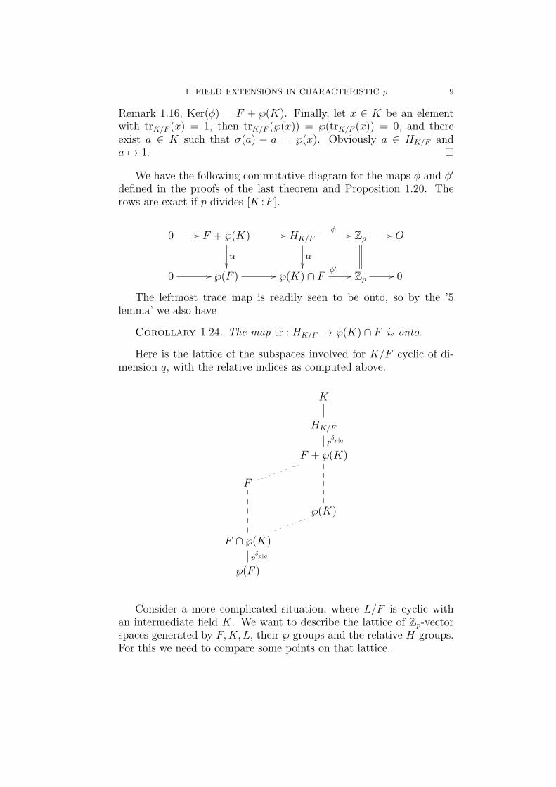
Corollary 1.24. The map tr : HK/F → ℘(K) ∩ F is onto.
Here is the lattice of the subspaces involved for K/F cyclic of di-mension q, with the relative indices as computed above.
K
HK/F
pδp|q
F + ℘(K)
F
℘(K)
F ∩ ℘(K)
pδp|q
℘(F )
Consider a more complicated situation, where L/F is cyclic withan intermediate field K. We want to describe the lattice of Zp-vectorspaces generated by F,K,L, their ℘-groups and the relative H groups.For this we need to compare some points on that lattice.

10 1. p-ALGEBRAS
Recall that the lattice of subspaces of a given space is modular, i.e.,for every three subspaces A,B,C, if A ⊆ C then
A+ (B ∩ C) = (A+B) ∩ C.In this case we write A+B ∩ C and omit parenthesis.
Theorem 1.25. Let L/F be a cyclic extension, with F ⊆ K ⊆ L.Then the following equalities hold:
a. K ∩HL/F = HK/F .b. HK/F ∩ ℘(L) = K ∩ ℘(L).c. HL/F +K = HL/K.d. ℘(L) +HK/F = ℘(L) +K ∩HL/F .e. HK/F + ℘(L) = F + ℘(L) if p | [L :K] or [K :F ] prime to p, and
[HK/F + ℘(L) :F + ℘(L)] = p otherwise.f. ℘(L) ∩K ⊆ HK/F .g. F + ℘(L) ∩HK/F = F + ℘(L) ∩K.
Proof. Let m = [K :F ]. Denote by τ a generator of Gal(L/F ),and let θ : L → L denote the map θ = 1 + τ + · · · + τm−1. Note thatthe restriction of θ to K is trK/F , and that trL/K θ = trL/F . Also,(τm − 1) = θ(τ − 1).
a. The inclusion K ∩HL/F ⊇ HK/F is trivial. Let a ∈ K ∩HL/F .Then τ(a)−a = ℘(l) for some l ∈ L. Compute that 0 = trK/F (τa−a) =trK/F℘(l) = ℘(θl), so that θl ∈ Zp ⊆ F . Now τm(l)−l = τ(θl)−θl = 0,so that l ∈ K and a ∈ HK/F .
b. By part a., HK/F ∩ ℘(L) = HL/F ∩ K ∩ ℘(L) = K ∩ ℘(L) as℘(L) ⊆ HL/F .
c. The inclusion HL/F +K ⊆ HL/K is trivial. Let a ∈ HL/K , thenτm(a)− a = ℘(l) for some l ∈ L. As before ℘(trK/L(l)) = trK/L℘(l) =trK/L(τ
m(a) − a) = 0 so trK/L(l) ∈ Zp ⊆ F . By Remark 1.22, wecan find l1 ∈ L such that trL/F (l1) = trL/K(l). Since trL/Kθ = trL/F ,we have that trL/K(l − θl1) = trL/K l − trL/F l1 = 0, and there is somer ∈ L such that l − θl1 = (τm − 1)(r). Let l0 = l1 + (τ − 1)(r),then θl0 = θl1 + θ(τ − 1)r = θl1 + (τm − 1)(r) = l. Compute thattrL/F℘(l0) = ℘(trL/F l1) = ℘(trL/K l) = trL/K(τ
ma− a) = 0. Thus thereis some b ∈ L such that τ(b) − b = ℘(l0), so that b ∈ HL/F . Now,τm(b)− b = θ(τ − 1)(b) = θ℘(l0) = ℘(θl0) = ℘(l) = τm(a)− a, so thatτm(a− b) = a− b, and a− b ∈ K. Thus a ∈ K +HL/F , as asserted.
d. Immediate from part a.

1. FIELD EXTENSIONS IN CHARACTERISTIC p 11
e. Consider the spaces K + ℘(L) and HL/F . Their sum is, by partc., equal to HL/K + ℘(L) = HL/K . By part d., their intersection isHK/F + ℘(L). Thus HL/F/(HK/F + ℘(L))∼=HL/K/(K + ℘(L)). Thisquotient is of size pδp|[L:K] by Corollary 1.18 and Theorem 1.23. Fromthe same reasons
∣∣HL/F/(F + ℘(L))∣∣ = pδp|[L:F ] . Dividing, we find out
that [HK/F + ℘(L) :F + ℘(L)] is as asserted.
f. Let ℘(l) ∈ K for some l ∈ L. Then 0 = (τm − 1)℘(l) =℘((τm − 1)l), so that (τm − 1)l ∈ Zp ⊆ F . Thus (τm − 1)(τ − 1)l =(τ−1)(τm−1)l = 0, and (τ−1)l ∈ K. Now, τ℘(l)−℘(l) = ℘((τ−1)l) ∈℘(K), so that ℘(l) ∈ HK/F .
g. The inclusion F + ℘(L) ∩HK/F ∩ F + ℘(L) ∩K is obvious, andthe other direction follows from part f.
With all these facts put together, we get the following lattice (inwhich the intersection and sum of spaces always appears in its properplace). We set ϵ1p to be p if [L :K] is prime to p and [K :F ] is divisibleby p, and 1 otherwise. Similarly ϵp1 = p if [L :K] is divisible by p and[K :F ] prime to p, and 1 otherwise. Also, ϵpp = p if [L :K] and [K :F ]are both divisible by p, and 1 otherwise. Finally, we set ϵp = ϵp1ϵ
pp, and
ϵp = ϵ1pϵpp. The numbers in the diagram denote relative indices.

12 1. p-ALGEBRAS
L
HL/K
ϵpnnnnnn
n
;;
;;
;;
K + ℘(L)
AA
AA
AA
A
K
EE
EE
EE
EE HL/F
ϵprrrrr
HK/F + ℘(L)ϵ1p
HK/F
ϵ1p
F + ℘(L)
;;;;
;;;;
;;;;
;;;;
;;;;
;;;;
F + ℘(L) ∩K
ϵppllll
lll
EEEE
EEEE
EEEE
EE
EEEE
EEEE
EEEE
EE
F + ℘(K)
EEEE
EEEE
EEEE
EE
EEEE
EEEE
EEEE
EE℘(L)
F
22222222222
22222222222 K ∩ ℘(L)
ϵppllll
lll
℘(K) + F ∩ ℘(L)ϵp1
F ∩ ℘(L)ϵp1
℘(K)
F ∩ ℘(K)ϵp
℘(F )
1.5. Counting Cyclic Extensions. In subsection 1.2 it was men-tioned that Galois extensions of F with Galois group Zd
p are parame-terized by d-dimensional subspaces of F/℘(F ). If
dF = dimZp F/℘(F )
is finite, we can actually count the extensions. The simplest exampleis where F is finite — then dF = 1. Note that by [15, Prop. 4.4.8], thep-part of the Brauer group Br(F ) is trivial when dF is finite.
Let K/F be a cyclic extension. The lines of K/℘(K) correspond to
cyclic extensions of dimension p over K, and there are pdK−1p−1 such ex-
tensions. Similarly, by Corollary 1.15 there are exactly[HK/F :℘(K)]−1
p−1 =

1. FIELD EXTENSIONS IN CHARACTERISTIC p 13
pdF−1p−1 central Galois extensions of F which are p-dimensional over K
(the equality follows from Theorem 1.23).The possible Galois groups for these extensions over F are Zp ×Zq
and Zpq (the two types coincide if q is prime to p). By Theorem 1.19,extensions of the first type correspond to the classes (F +℘(K))/℘(K).
The following follows from Proposition 1.20.
Remark 1.26.
[F + ℘(K) :℘(K)] = pdF−δp|q .
Proof.
[F + ℘(K) :℘(K)] = [F :F ∩ ℘(K)]
= [F :℘(F )]/[F ∩ ℘(K) :℘(F )]
= pdF−δp|q .
Corollary 1.27. Suppose K/F is a cyclic extension. From Re-mark 1.26 we have that
[F + ℘(K) :℘(K)] = pdF−δp|q ,
so that there are exactly pdF−δp|q−1
p−1 Galois extensions L of F , containing
K as a subfield, such that Gal(L/F )∼=Zp × Zq.
For example, if dF = 1, let K be the only extension of dimension p.Then F ⊆ ℘(K), and, as expected, there are no extensions of F withGalois group Zp × Zp.
Now assume p | q, and count the extensions of the second type (thosewhich are cyclic over F ). From Theorem 1.23 we have
Corollary 1.28. Suppose K/F is cyclic of dimension divisible byp.
The number of extensions of K which are cyclic of dimension p ·[K :F ] over F , equals pdF−1.
Proof. By Remark 1.26 and Theorem 1.23, we have that [HK/F :℘(K)] =[HK/F :F + ℘(K)] · [F + ℘(K) :℘(K)] = pdF . Now subtract the num-ber of extensions with Galois group Zp × Zq (Corollary 1.27) from thenumber of central Galois extensions:
[HK/F :℘(K)]− 1
p− 1− pdF−1 − 1
p− 1=pdF − pdF−1
p− 1= pdF−1.

14 1. p-ALGEBRAS
In particular, if F has at least one cyclic extension, then pdF−1 ≥ 1,and we can inductively define a chain of cyclic extensions of F ,
F = F0 ⊆ F1 ⊆ F2 ⊆ . . .
and inspect F = ∪Fi:
Corollary 1.29. Every cyclic extension K/F of dimension a power
of p is embedded in an extension F /F such that Gal(F /F ) = lim← Zpn
is the Abelian pro-p group of rank 1 (i.e. the additive group of the p-adicintegers).
This last corollary is usually deduced by the construction of Wittvectors, e.g. [14].
In particular, if dF = 1 then pdF−1 = 1 and we have
Corollary 1.30. Suppose F has a unique cyclic extension of orderp.
Then F has a unique cyclic extension of any order pn. Moreover,F has a unique extension F with Gal(F /F ) = lim← Zpn.
Remark 1.31. In the case dF = 1, the field F has no cyclic exten-sions of dimension p.
Proof. Let θ ∈ F . Then θ ∈ Fi for some i, and λp − λ − θ has asolution in Fi+1, and thus in F .
Corollary 1.32. Let K be a separably closed field of characteristicp. Then the absolute Galois group Λ = Gal(K/Zp) has no finite p-subgroups.
Proof. Otherwise, let σ ∈ Λ be an element of order p. ThenF = Kσ has a cyclic extension, so that dF ≥ 1 and by the theoremdK ≥ 1. But dK = 0 by assumption.
The information in Corollary 1.28 can also be interpreted in termsof subgroup growth of the absolute Galois group of F , denoted by ΓF .For a groupG, let Cn(G) denote the number of normal subgroupsNGof index n with cyclic quotient group.
Theorem 1.33.
Cpn(ΓF ) =pdF − 1
p− 1p(dF−1)(n−1).
In particular,logCpn (ΓF )
log pn−→ dF − 1.

1. FIELD EXTENSIONS IN CHARACTERISTIC p 15
Proof. Every normal subgroup with quotient ΓF/N = Zpn is con-tained in exactly one normal subgroup with quotient Zpn−1 , so that
Cpn(ΓF ) = Cpn−1(ΓF ) · pdF−1. But Cp(ΓF ) =pdF−1p−1 by definition of dF ,
so the result follows by induction. 1.6. Going Up One Stage. We now discuss the number of p-
cyclic extensions of F and K when F ⊆ K. We treat two easy cases(K/F Galois of dimension prime to p, or K/F purely inseparable), anda harder and more fruitful one, when K/F is itself cyclic of dimensionp.
Proposition 1.34. If K/F is Galois and [K :F ] is prime to p,then dF ≤ dK.
Proof. The map L 7→ L⊗FK (taking cyclic extensions of dimen-sion p over F to cyclic extensions of the same dimension over K) isinjective, since the (normal) subgroup of elements of prime-to-p orderin Zp ×Gal(K/F ) is unique.
Theorem 1.35. Let K/F be a purely inseparable extension. Thena. K = F + ℘(K).b. ℘(K) ∩ F = ℘(F ).c. dK = dF .
Proof. We may assume K/F is of exponent p (and then use in-duction).
a. For every k ∈ K, k = kp − (kp − k) ∈ F + ℘(K).b. If kp − k ∈ F , then k ∈ Kp + F = F .c. K/℘(K) = (F + ℘(K))/℘(K)∼=F/(℘(K) ∩ F ) = F/℘(F ). And now, the cyclic case. The result we give here follows from
Witt’s theorem that the Galois group of the maximal pro-p extensionover F is a free pro-p group [25, Cor. 3.2]. Since our theorem countssubgroups of index p, it is equivalent to Witt’s theorem for the finitely-generated case by a result of A. Lubotzky.
Theorem 1.36. Let K = F [u], up − u = θ ∈ F , be a cyclic exten-sion of dimension p over F . Then
dK = p(dF − 1) + 1.
Proof. In order to compute dK = logp |K/℘(K)| we construct aset of representatives for K/℘(K).
Since θ ∈ ℘(F ), Θ = (Zpθ + ℘(F ))/℘(F ) is a subgroup of orderp of F/℘(F ). Pick a set BF of representatives for the quotient group(F/℘(F ))/Θ, so that BF + Zpθ is a complete set of representatives forF/℘(F ). In particular, pdF = |F/℘(F )| = p|BF |.

16 1. p-ALGEBRAS
Another way to put it: every element f ∈ F is expressible in theform
(2) f = gp − g + b+ iθ
for g ∈ F, b ∈ BF , i ∈ Zp, where b, i are unique (and g is unique up toadding integers). In a more graphic form, F = ℘(F )⊕BF ⊕ Zpθ.
Let BK = BF +BFu+ · · ·+BFup−1 +Zpθu
p−1. We claim that BK
is a complete set of representatives for K/℘(K). Let fK =∑p−1
i=0 fiui ∈
F [u] be an arbitrary element of K. We shall use reverse induction onthe degree of fK in order to show that fK is expressible as
(3) fK = ℘(gK) + bK
for unique bK ∈ BK , and unique gK ∈ K up to adding integers.Write bK =
∑p−1i=0 biu
i + jθup−1, bi ∈ BF , and gK =∑p−1
i=0 giui, gi ∈
F . Note that in general, the upper monomial of (ui)p = (up)i = (u+θ)i
(considered as a polynomial in u over F ) is ui. Hence, the coefficientof up−1 in gK
p − gK is gp−1p − gp−1. Comparing coefficients of up−1 in
(3), we have the equation
(4) fp−1 = gp−1p − gp−1 + bp−1 + jθ,
which by (2) has a solution with unique bp−1 and j, and gp−1 uniqueup to adding integers.
Now let i ≤ p−1. Suppose j ∈ Zp, bp−1, . . . , bi ∈ BF , gp−1, . . . , gi+1 ∈F are fixed, and gi is fixed up to adding integers. Write gi = gi0 + ji,where gi0 is already fixed and ji ∈ Zp is yet to be determined. We solvefor bi−1,ji, and gi−1 up to integers, by comparing coefficients of ui−1
after removing the fixed part from (3). If h ∈ K = F [u], we denote by[ui]h the coefficient of ui in h.
Let f ′i−1 = [ui−1](fK − ℘(∑p−1
l=i+1 glul)), and compute using (3):

1. FIELD EXTENSIONS IN CHARACTERISTIC p 17
f ′i−1 = [ui−1](fK − ℘(
p−1∑l=i+1
glul))
= [ui−1](℘(i∑
l=0
glul) +
p−1∑i=0
blul + jθup−1)
= [ui−1](i∑
l=0
(gpl ulp − glu
l)) + bi−1
= [ui−1](i∑
l=0
gpl (u+ θ)l −i∑
l=0
glul) + bi−1
= [ui−1](i∑
l=i−1
gpl (u+ θ)l −i∑
l=i−1
glul) + bi−1
= [ui−1](gpi (u+ θ)i − giui + gpi−1(u+ θ)i−1 − gi−1u
i−1) + bi−1
= [ui−1](igpi θui−1 + (gpi−1 − gi−1)u
i−1) + bi−1
= (gpi−1 − gi−1) + i(gi0p + ji)θ + bi−1
Subtracting igpi0θ, we get the equation
(5) f ′i−1 − igi0θ = gpi−1 − gi−1 + bi−1 + ijiθ.
By the choice of BF this equation has a solution, with unique bi−1 ∈BF and ji ∈ Zp, and gi−1 unique up to adding integers. After fixing jiwe know gi, and the next induction step can be performed.
We have shown that BK is indeed a basis for K/℘K, so that pdK =|K/℘(K)| = |BK | = |BF |pp = pp(dF−1)+1, and we are done.
Corollary 1.37. If F = F0 ⊂ · · · ⊂ Fn is a chain of cyclicextensions of dimension p, then dFn = pn(dF − 1) + 1.
This result too is related to subgroup growth of Γ = ΓF , the ab-solute Galois group of F . Let Sn(G) denote the number of subnormalsubgroups of index n in G.
Theorem 1.38.
Spn(Γ) <
(p
p− 1
)n
ppn−1p−1
(dF−1).
In particular,log logSpn (Γ)
log pn< 1 + o(1) whenever dF is finite.
18 1. p-ALGEBRAS
Proof. Note that if N ≤ G is a subnormal group of p-power index,then N = Nt Nt−1 . . . N1 N0 = G, where Ni/Ni−1 is of orderp. In particular, Spn(G) is bounded by the sum of numbers of normalsubgroups of index p of all the subnormal subgroups of index pn−1 in
G. By the last corollary we have that Spn(Γ) ≤ Spn−1(Γ)ppn(dF−1)+1−1
p−1 ,
and by induction
Spn(Γ) ≤ Πn−1i=0
ppi(dF−1)+1 − 1
p− 1
< Πn−1i=0
ppi(dF−1)+1
p− 1
= (p− 1)−npn+(dF−1)(1+p+···+pn−1).
Remark 1.39. In the special case where F has no prime-to-p ex-tensions, Γ is a pro-p group and every subgroup is subnormal. In thiscase Spn(Γ) is the number of subgroups of index pn.
2. Cyclic p-Algebras
A simple algebra A/F is cyclic if it contains a maximal subfieldK which is cyclic over F . See [22] for a survey of the history of cyclicalgebras.
The main structure theorem on p-algebras (algebras over F withdeg(A) a power of char(F ) = p) is that every p-algebra is similar (inthe Brauer group) to a cyclic algebra ([1, VII.31], [15, 4.5.7]). Non-cyclic p-algebras (with degree ≥ p2) were first constructed by Amitsurand Saltman [4].
If exp(A) = p, then A is similar to a tensor product of cyclic al-gebras of degree p [15, 4.2.17]. It follows that the exponent-p partof Br(F ) is generated by (the classes of) cyclic algebras of degree p.Whether or not every p-algebra of degree p is cyclic is still wide open.
Every p-algebra A has a finite dimensional purely inseparable sub-field S/F [15, 4.1.10], and exp(A) equals the minimal exponent of sucha field over F . If S = S ′[u] where up ∈ S ′, and [F [u] :F ] = pe, and S ′
does not split A, then A⊗C is split by S ′ for C a cyclic p-algebra ofdegree pe over F [15, 4.2.11].
This is used as an induction mechanism to show, for example, thefollowing. If [F ∗ :F ∗p] = pd, then A is similar to a product of at mostd cyclic algebras of degree p (since F 1/p splits A, and is of dimensionpd over F ). More generally we have

2. CYCLIC p-ALGEBRAS 19
Remark 2.1. Suppose exp(A) = pe, where [F ∗ :F ∗p] = pd. ThenA is split by F 1/pe , which has dimension pde over F . It follows that Ais similar to a product of at most de cyclic algebras, at most d of anydegree pi (i = 1 . . . e). At least one cyclic algebra of degree pe must bepresent.
If S/F is purely inseparable, then the map [A] 7→ [A⊗S] from Br(F )to Br(S) is surjective [15, 4.1.5]. In particular for S = F 1/p, we havethat the map [A] 7→ [A⊗F 1/p] = [A]p is surjective, so that Br(F ) isp-divisible. This is an important step in showing that every p-algebrais similar to a product of cyclic algebras.
We now discuss the presentation of cyclic algebras of degree p bymeans of generators and relations. We give full details of this oldconstruction, in order to make the computations more accessible in thesequel.
Let A be a cyclic p-algebra of degree p, with maximal subfield K,generated by x ∈ K such that xp − x = a ∈ F (Theorem 1.7). Theautomorphism σ ∈ Gal(K/F ) acts on K by σ(x) = x+ 1. By Skolem-Noether, there exists an element y ∈ A such that yxy−1 = x+ 1.
Lemma 2.2. F [y] is an inseparable extension of degree p over F ,and as a maximal subfield, it splits A.
Proof. It is easy to compute that yjxy−j = x+j, so that for everyf(λ) ∈ F [λ], xf(y) − f(y)x = −yf ′(y), where f ′ denote the standardderivative of f .
Now let g(λ) ∈ F [λ] be the minimal polynomial of y over F . Sinceg(y) = 0, we also have g′(y) = 0. But deg(g′) < deg(g), so we musthave g′(λ) = 0, and p | deg(g). Thus [F [y] :F ] ≥ p, but since F [y] is
commutative, [F [y] :F ] ≤√[A :F ] = p, so that [F [y] :F ] = p. F [y] is
inseparable since g(λ) = λp − (yp).
We have seen that no element of F [y]−F commutes with x, so thatF [x] ∩ F [y] = F . Counting dimensions we see that F [x, y] = A. Nowyp commutes with x and with y, so that b = yp ∈ F .
The relations
xp − x = a, yp = b, yxy−1 = x+ 1(6)
fully determine the multiplication in A, and we may use them to definethe symbol p-algebra
[a, b) = F [x, y : xp − x = a, yp = b, yx = xy + y].
Note that it is always central simple over F .

20 1. p-ALGEBRAS
As mentioned above, the classes of [a, b), a, b ∈ F , generate pBr(F )(the exponent-p part of Br(F )). We now give a list of relations satisfiedby these generators.
Lemma 2.3. If a ∈ ℘(F ) = up − u : u ∈ F, or b ∈ (F ∗)p, then[a, b) is split.
Proof. Since [a, b) is of prime degree, it is either a division algebraor the split algebra Mp(F ).
Thus, it is enough to show that [a, b) is not a division algebra. In-deed, if λp − λ−a is reducible over F , let α ∈ F be a root (Proposition1.5). Then Πp−1
i=0 (x− α− i) = ℘(x− α) = a− a = 0, and we have zerodivisors. If b = βp for β ∈ F , then (β−1y − 1)p = 0 and again we havezero divisors.
The next theorem is responsible for the other identities. Its proofwill be used in section 4.
Theorem 2.4. a. [a1, b1)⊗ [a2, b2)∼=[a1 + a2, b1)⊗ [a2, b−11 b2).
b. [a1, b1)⊗ [a2, b2)∼=[a1, b1b2)⊗ [a2 − a1, b2).
Proof. The left hand sideR is generated in both cases by x1, x2, y1, y2,satisfying xi
p − xi = ai, ypi = bi, x1x2 = x2x1, y1y2 = y2y1, yixjy
−1i =
xj + δij.a. It is easy to check that R1 = F [x1+x2, y1] and R2 = F [x2, y
−11 y2]
are commuting subalgebras which generate R, R1∼=[a1 + a2, b1), and
R2∼=[a2, b
−11 b2).
b. The same argument, with R1 = F [x1, y1y2], R2 = F [x2 − x1, y2].
Corollary 2.5. a. [a1, b)⊗ [a2, b)∼=[a1 + a2, b)⊗Mp(F ).b. [a, b1)⊗ [a, b2)∼=[a, b1b2)⊗Mp(F ).
Proof. Substitute b1 = b2 in Theorem 2.4.a, a1 = a2 in 2.4.b, anduse 2.3.
A final computation:
Remark 2.6. [a, a)∼=Mp(F ).
Proof. Consider the elements x, x−1y in [a, a) = F [x, y : xp − x =yp = a, yxy−1 = x + 1]. They satisfy xp − x = a, (x−1y)x(x−1y)−1 =x−1(yxy−1)x = x−1(x+ 1)x = x+ 1, and finally,
(x−1y)p = NF [x]/F (x)−1yp = a−1a = 1.
Thus [a, a)∼=[a, 1)∼=Mp(F ).

3. PRESENTATION FOR pBr(F ) 21
Did we miss an identity? In the next section it will be shown thatthe results 2.3,2.5 and 2.6 are enough to prove any relation satisfied byp-symbols.
3. Presentation for pBr(F )
3.1. The Merkurjev-Suslin Theorem. Let R be a ring, andlet GL(R) denote the direct limit of the groups GLn(R) of invertiblen × n matrices, under the canonical injections GLn(R) → GLn+1(R)by A 7→ A⊕ 1.
The generators eij(r) = 1 + reij (r ∈ R, i, j ≥ 1) of GL(R) satisfycertain identities, e.g. eij(r)ejk(s) = eik(r+ s). It is not surprising thatsome relations depend on the arithmetic of the ring R.
The Steinberg group St(R) of R is defined by generators xij(r),and certain relations which apply to eij(r) over every ring R. K2(R)is defined as the kernel of the map xij(r) 7→ eij(r) from St(R) ontoGL(R), and is a measure of how ’general’ is the ring from an arith-metical point of view. It turns out that K2(R) is always an Abeliangroup, and that K2 : R 7→ K2(R) is a functor from the category of ringsto the category of abelian groups.
Matsumoto has proved (cf. [26, Thm. 4.3.15]) that if F is a field(of arbitrary characteristic), then K2(F ) is the abelian group generatedby the symbols a, b (a, b ∈ F ∗), subject to the relations
a, b1+ a, b2 = a, b1b2,
a1, b+ a2, b = a1a2, b,a, 1− a = 0.
The connection to simple algebras is evident, since symbol algebrasin characteristic 0 obey the same rules. For every n, if charF is primeto n and F has primitive n’th roots of unity, there is a canonical mapfrom K2(F ) to nBr(F ), sending the symbol a, b to the cyclic algebra(a, b)n;F = F [x, y|xn = a, yn = b, yxy−1 = ρx].
The precise result has very far reaching consequences.
Theorem 3.1 (Merkurjev-Suslin [24]). Let n be an integer, and Fa field with characteristic prime to n, containing n’th roots of unity.
Then the natural map sending a, b to the symbol algebra (a, b)ninduces an isomorphism K2(F )/nK2(F ) → nBr(F ).
Essentially, this is a description of nBr(F ) in terms of generators(the cyclic algebras) and relations. As a result, if charF = 0 and F hasall the roots of unity, then K2(F )∼=Br(F ) (since the above mentionedmaps are coherent).
22 1. p-ALGEBRAS
There are partial results for the case where F does not have rootsof unity. Merkurjev [23] has proved that if q is a prime = charF ,then qBr(F ) is generated by the classes of algebras of index q. Also if[F [µq] :F ] ≤ 3, then qBr(F ) is generated by the classes of cyclic algebrasof degree q.
In connection with this result, it was proved by Merkurjev that inthe case [E :F ] ≤ 3, K2(E) is generated by the symbols a, β, a ∈ E,β ∈ F . The same is true if F has no prime-to-[E :F ] extensions [7].
Even today, after several simplifications of the proof have beenmade, the Merkurjev-Suslin theorem is still considered very hard. Themost difficult part is a K2 analog for Hilbert’s theorem 90: if K/Fis cyclic, Gal(K/F ) = ⟨σ⟩, and r ∈ K2(K) satisfies
∑σir = 0, then
r = σs−s for some s ∈ K2(K). The proofs of this result use heavy ma-chinery from etale cohomology, including higherK functors, the Braun-Gerstein-Quillen spectral sequence, and analysis of Chern classes (cf.[40]). A proof can be found in [38]. We discuss Hilbert’s theorem 90for subgroups of prime exponent of Br(K) in Section 6.
Motivated by the description of nBr(F ) by generators and relationsfor the prime-to-p case, we give in this section a similar description for
pBr(F ) where p = charF . The presentation we describe below was firstproved by Teichmuller. In a more modern language, it can be derivedfrom the Cartier map Ω1
F → Ω1F/d(Ω
0F ) defined by xdy
y7→ (xp − x)dy
y,
cf. [17]. Our proof is rather similar to that of Teichmuller, and weinclude it for completeness.
3.2. Generators and Relations for pBr(F ). Let F be a field ofcharacteristic p.
In this subsection we give a presentation of pBr(F ) in terms ofgenerators and relations. As generators we use the p-cyclic algebras— they generate pBr(F ) by Albert’s structure theory for p-algebras,proved back in the 40’s.
Definition 3.2. K2(F ) is defined as the free abelian group gen-erated by all formal p-symbols [a, b (a, b ∈ F , b = 0), subject to thefollowing relations (a, a1, a2, b1, b2 ∈ F , b, b1, b2 = 0):
[a1 + a2, b = [a1, b+ [a2, b(7)
[a, b1b2 = [a, b1+ [a, b2(8)
[b, b = 0(9)
[ap − a, b = 0.(10)

3. PRESENTATION FOR pBr(F ) 23
Remark 3.3. From Equations (7) and (8), we see that [a, bp =p[a, b = [pa, b = [0, b = 0.
Another useful computation is given by
Remark 3.4. For every a, b, c ∈ F , b, c = 0,
[apbc, b = −[apbc, c(11)
Proof. If a = 0 we are done. Otherwise, compute that [apbc, b =[apbc, b − [apbc, apbc = [apbc, 1
cap = −[apbc, c.
It is evident that (a, b) → [a, b defines a map from (F,+)⊗ZpF ∗
onto K2(F ). Actually, this induces a map of abelian groups,
F/℘(F )⊗ZF∗/F ∗p → K2(F ),
whose kernel is generated by the couples (a, a) (cf. [10, Lemma 11.14]).Define a map RF : K2(F ) → pBr(F ) by RF : [a, b 7→ [a, b), where
[a, b) = F [x, y : xp−x = a, yp = b, yx = (x+1)y] is the cyclic p-algebra.This map is a well defined homomorphism by the basic computationalrules satisfied by cyclic p-algebras (Corollary 2.5 and Remark 2.6).
RF is onto by Albert’s structure theory, so it remains to show thatRF is one-to-one.
We start with an example for values of a for which [a, b 7→ 0.
Lemma 3.5. If a = γp0 − γ0 +∑p−1
i=1 γpi b
i for γi ∈ F , then [a, b = 0.
Proof. [u, v = [u, v − [u, u = [u, vu. Now compute:
[a, b = [γp0 − γ0 +
p−1∑i=1
γpi bi, b
= [γp0 − γ0, b+p−1∑i=1
[γpi bi, b
=
p−1∑i=1
[γpi bi, b
=
p−1∑i=1
[1
iγpi b
i, bi
= 0.
where the last equality follows from Remark 3.4 (with c = 1).
It turns out that this example is the most general one:
24 1. p-ALGEBRAS
Fact 3.6. LetB be an C-algbera, and C a commutative subalgebra.Let δ : C → C be the derivation induced by z ∈ B: zf − fz = δ(f) forall f ∈ C.
Then (z + f)p = zp + fp + δp−1(f).
Theorem 3.7 (Teichmuller [39]). If [a, b) splits then a = γp0 −γ0+∑p−1i=1 γ
pi b
i for some γi ∈ F .
Proof. By assumption [a, b) ∼= Mp(F ) ∼= [0, b), so there are x, y ∈Mp(F ) such that xp − x = a, yp = b and yx = (x + 1)y, and z′, y′ ∈Mp(F ) such that y′p = b, z′p − z′ = 0 and y′z′ = (z′ + 1)y′. But sinceF [y] ∼= F [y′], there is some t ∈ Mp(F ) such that y = ty′t−1. Settingz = tz′t−1, we have that zp − z = 0 and yz = (z + 1)y.
Now y(x − z) = ((x + 1) − (z + 1))y = (x − z)y, so that x − zcommutes with y and x− z ∈ CMp(F )F [y] = F [y]. Thus, x− z = f(y)
for some polynomial f(λ) ∈ F [λ]. Write f(y) =∑p−1
i=0 γiyi.
In 3.6 take B =Mp(F ) and C = F [y]. The derivation δ induced byz satisfies δ(y) = −y, and more generally δ(f(y)) = −yf ′ where f 7→ f ′
is the ordinary derivation of polynomials. δp−1(yi) = (−i)p−1yi = yi
for every i > 0, so that δp−1(f(y)) = f(y)− f(0).We can now compute: a + z + f(y) = a + x = xp = (z + f(y))p =
zp+f(y)p+f(y)−f(0), so that a = f(y)p−f(0) =∑p−1
i=0 γpi b
i−γ0.
Remark 3.8. Let F p ⊆ F be the subfield of all p−powers in F . Ifa = γp0 − γ0 +
∑p−1i=1 γ
pi b
i then γ0 ∈ F p(a, b).
For the induction step we need the following lemma.
Lemma 3.9. If [a1, b1) ⊗ · · · ⊗ [an, bn) splits, then [a1, b1 + · · · +[an, bn can be written as a sum of n− 1 symbols in K2(F ).
Proof. Let S = F [b1/p2 , . . . , b
1/pn ], a purely inseparable extension of
F . Obviously S splits [ai, bi) for all i = 2, . . . , n, but since [a1, b1) ⊗· · · ⊗ [an, bn) is split, S splits [a1, b1) too. By Theorem 3.7, there existγ0, . . . , γp−1 ∈ S with a1 = γp0 − γ0 +
∑p−1i=1 γ
pi b
i1, where by the above
remark γ0 ∈ Sp(a1, b1)=F.
Let G = Zn−1p be the split abelian group of exponent p. If g ∈ G,
gj is the j’th component of g (j = 2, . . . , n).Define a function β : G → S by βg = (bg22 . . . bgnn )1/p. The elements
βg : g ∈ G form a basis for S over F . Of course, βpg = bg22 . . . bgnn ∈ F .
For i = 1, . . . , p − 1, write γi =∑
g∈G γi,gβg, γi,g ∈ F . Then γpi =∑g∈G γ
pi,gβ
pg . Now compute:

3. PRESENTATION FOR pBr(F ) 25
[a1, b1 = [γp0 − γ0 +
p−1∑i=1
γpi bi1, b1 =
= [γp0 − γ0, b1+p−1∑i=1
[γpi bi1, b1 =
=
p−1∑i=1
∑g∈G
[γpi,gβpgb
i1, b1 =
=
p−1∑i=1
∑g∈G
[1
iγpi,gβ
pgb
i1, b
i1 =
= −p−1∑i=1
∑g∈G
[1
iγpi,gβ
pgb
i1, β
pg,
the last equality follows from Remark 3.4 with c = βpg .
Now compute that
[a1, b1 + [a2, b2+ · · ·+ [an, bn =
= −p−1∑i=1
∑g∈G
[1
iγpi,gβ
pgb
i1, b
g22 . . . bgnn + [a2, b2+ · · ·+ [an, bn =
= −n∑
j=2
p−1∑i=1
∑g∈G
[gjiγpi,gβ
pgb
i1, bj+ [a2, b2+ · · ·+ [an, bn =
=n∑
j=2
[aj −p−1∑i=1
∑g∈G
gjiγpi,gb
i1β
pg , bj.
Thus [a1, b1+ · · ·+[an, bn is the sum of n−1 symbols, as asserted.
Theorem 3.10. K2(F )∼=pBr(F ).
Proof. We need to show that RF is one-to-one, that is, that[a1, b1) ⊗ · · · ⊗ [an, bn) ∼ F implies [a1, b1 + · · · + [an, bn = 0. Thecase n = 1 is Teichmuller’s Theorem 3.7 (combined with Lemma 3.5).
Assume the assertion holds for sums of n− 1 symbols, and suppose[a1, b1+ · · ·+[an, bn 7→ 0, i.e. [a1, b1)⊗· · ·⊗ [an, bn) splits. By Lemma3.9, [a1, b1+ · · ·+ [an, bn is a sum of n− 1 symbols with split image,so by the induction hypothesis [a1, b1+ · · ·+ [an, bn = 0.

26 1. p-ALGEBRAS
4. Generators of p-Algebras
Among the basic notions in the study of the automorphisms groupof polynomial rings (e.g. over fields) are that of elementary automor-phisms, which are those who stabilize all but one of the variables, andthat of tame automorphisms, which are compositions of elementaryones.
In this section we suggest a similar notion as a tool to study thevariety of sets of standard generators of a p-algebra, which is a ten-sor product of symbol p-algebras. Since the automorphisms group of acentral simple algebra A is already known, we consider the possible pre-sentation of an algebra by standard generators, and use isomorphismsas a device holding two presentations of an algebra at the same time.
This approach is motivated by the fact that axioms (7)–(10) are allwe need to make computations in pBr(F ) (Theorem 3.10), and that thecorresponding relations between p-algebras are proved (in 2.3–2.6) interms of explicit generators. It follows that every equality in pBr(F ) canbe explained in terms of simple changes of generators, if we add enoughmatrices in both sides. A natural question is how many matrices areneeded in order to make room for the elementary changes. An answer(and precise formulation of the question) are given in Theorem 4.16.
The standard presentations of symbol p-algebras were describedin Section 2. In subsection 4.1 we discuss the elementary switchesbetween standard sets of generators of symbol p-algebras, define tameisomorphisms, and prove some basic facts about sets of generators.This is generalized later to tensor products of several symbol p-algebras.
In the second subsection we prove (Theorem 4.9) that if two p-symbols are equal in the Brauer group, then there is a way to rewriteevery symbol as sum of at most p − 1 symbols, such that the isomor-phism becomes, in a sense, obvious.
This result is used in the third subsection to show that if [a, b)∼=[a′, b′)are two presentations of the same algebra, then there is a chain of ele-mentary switches of sets of generators which goes from the presentation[a, b)⊗Mp(F )
⊗2(p−2) to [a′, b′)⊗Mp(F )⊗2(p−2).
4.1. Generators of Cyclic p-Algebras. Let A/F be a cyclicp-algebra of degree p.
Definition 4.1. x, y ∈ A form a standard couple of generators(SCOG) of A if F [x, y] = A, and
(12) yxy−1 = x+ 1.
It should be noted that (12) gives a presentation of A as a p-symbol,A = [xp − x, yp), by the following easy computation.

4. GENERATORS OF p-ALGEBRAS 27
Lemma 4.2. If x, y form a SCOG, then x satisfies
(13) xp − x ∈ F
and y satisfies
(14) yp ∈ F
Proof. From (12) compute that ypxy−p = x, and that y(xp − x)y−1 =xp − x. It follows that xp − x, yp ∈ CA(F [x, y]) = Cent(A) = F .
Write A = [a, b) where a = xp − x and b = yp. Note that for anyt ∈ A, the SCOG txt−1, tyt−1 gives the same presentation. Since weare interested mainly in the symbols, we identify two SCOGs if theyare conjugate.
Remark 4.3. If x, y and x′, y′ are two SCOGs of A, with xp − x =x′p − x′ and yp = y′p, then by Skolem-Noether there is a conjugationthat takes x → x′ and y → y′. In other words, there is a one-to-onecorrespondence between SCOGs-up-to-conjugation, and presentationsof A as a symbol algebra.
For a symbol p-algebra A, let
XA = x ∈ A : xp − x ∈ F, x ∈ F,
YA = y ∈ A : yp ∈ F, y ∈ F.Every SCOG of A consists of x ∈ XA and y ∈ YA. Going from aSCOG x, y to a SCOG x′, y′ is called an elementary switch if x′ = xor y′ = y. This amounts to a change of presentation [a, b)∼=[a, b′) or[a, b)∼=[a′, b), and these are called elementary isomorphisms.
As a framework, we form the graph of SCOGs of A, with verticesthe ordered couples (x, y) ∈ XA × YA such that yxy−1 = x + 1, wherewe connect every two points (x, y), (x, y′) or (x, y), (x′, y). We work inthe quotient graph, identifying (x, y) and (x′, y′) if they are conjugatein A.
Let [a0, b0)∼=[an, bn) be an isomorphism, with respective SCOGs x, yand x′, y′.
Theorem 4.4. There is a path connecting the SCOGs x, y to x′, y′
in the graph, iff there is a chain of elementary isomorphisms
[a0, b0)∼=[a1, b1)∼= . . .∼=[an, bn).
Proof. A path in the graph corresponds to a chain of presenta-tions, where each step is an elementary isomorphism, i.e. one of thedefining constants remains the same.

28 1. p-ALGEBRAS
For the other direction, start from x, y, and replace one generatorat a time, until reaching a SCOG of [an, bn) (which is possibly differentfrom the target x′, y′). Now use Remark 4.3.
An isomorphism [a, b)∼=[a′, b′) is called tame, if it satisfies the con-ditions of the above theorem, i.e. it is a composition of elementaryisomorphisms.
Question 4.5. Let A be a symbol p-algebra. Is the isomorphismbetween any two presentations of A tame? In other words, is the graphof SCOGs of A connected?
Remark 4.6. The graph of SCOGs of Mp(F ) is connected.
Proof. Suppose [a, b)∼=Mp(F )∼=[a′, b′) are two presentations of thesplit algebra. Use
[a, b)∼=[0, b)∼=[0, b′)∼=[a′, b′).
It follows that if A∼=A′ is tame (where A,A′ are presentations of a
given algebra), then the isomorphism A⊗Mp(F )∼=A′⊗Mp(F ) is tametoo, and there is no need to specify the presentations of Mp(F ) inboth sides. This observation motivates the definition of stably-tameisomorphisms in the third subsection. In subsection 4.4 we answeraffirmatively Question 4.5 for p = 2.
We end this subsection with a closer look on elementary switches.First, we remark that for every x ∈ XA there is some y ∈ YA such
that x, y form a SCOG, and vice versa:
Remark 4.7. a. If x ∈ XA, then there is some y ∈ A such thatx, y form a SCOG of A.
b. If y ∈ YA, then there is some x ∈ A such that x, y form a SCOGof A.
Proof. a. By Remark 1.5, F [x] is either a subfield of A, or thesplit ring F×p. In both cases the automorphism induced by x 7→ x+ 1is inner (Skolem-Noether or the generalization to maximal separablecommutative subalgebras in [9]), say induced by y. y ∈ F [x], so thatF [x, y] = A.
b. This is [1, Theorem IV.17]. The following is a characterization of elementary switches for sym-
bol p-algebras, in terms of elements of the subfields involved.
Lemma 4.8. Let x, y be a SCOG of A.a. x, y1 is a SCOG iff y1 = ky for some k ∈ F [x].
4. GENERATORS OF p-ALGEBRAS 29
b. x1, y is a SCOG iff x1 = x+ u for some u ∈ F [y].
Proof. a. y1xy−11 = x+ 1 iff y1y
−1 ∈ CA(F [x]) = F [x].b. yx1y
−1 = x1 + 1 iff x1 − x ∈ CA(F [y]) = F [y].
4.2. The Connection Theorem.Suppose we have the equalities
[ck, b1 = [kck, b2,
for ck ∈ F (k = 1, . . . , p− 1). Then obviously
[
p−1∑k=1
ck, b1 = [
p−1∑k=1
kck, b2.
It turns out that every equality of p-symbols can be explained bythis observation.
Theorem 4.9 (Connection Theorem). Suppose [a1, b1 = [a2, b2,a1, b1, a2, b2 ∈ F .
Then there exist c1, . . . , cp−1 ∈ F such that
(15) [ck, b1 = [kck, b2
and
(16) [a1, b1 =
p−1∑k=1
[ck, b1 =
p−1∑k=1
[kck, b2 = [a2, b2.
Proof. If b2 is a p-power in F then we can take ck = 0, so assume
L = F [b1/p2 ] is a field. Since [a1, b1)⊗L∼=[a2, b2)⊗L ∼ L, we can apply
Theorem 3.7 and write a1 = γ0p − γ0 +
∑p−1i=1 γ
pi b
i1 for γi ∈ L. By
Remark 3.8, γ0 ∈ F . For every i > 0, write γi =∑p−1
j=0 γijbj/p2 , γij ∈ F .
Now let ck =∑−j/i≡k (mod p) γ
pijb
i1b
j2 (k = 0, 1, . . . , p− 1), and note that
[c0, b1 = 0. Then
[a1, b1 = [γ0p − γ0 +
p−1∑k=0
ck, b1 =
p−1∑k=1
[ck, b1.
Since ck ∈ F p·(b1b−k2 )+· · ·+F p·(b1b−k2 )p−1, we have that [ck, b1b−k2 = 0,
from which (15) follows. Finally,
[a2, b2 = [a1, b1 =∑
[ck, b1 =∑
[kck, b2
by assumption.
30 1. p-ALGEBRAS
4.3. Generators of Products of Symbols. Let A be a tensorproduct of symbol p-algebras.
Definition 4.10. Elements
(x1 x2 . . . xky1 y2 . . . yk
)∈ A form a stan-
dard vector of generators (SVOG) of A if x1, . . . , xk commute, y1, . . . , ykcommute, F [x1, . . . , xk, y1, . . . , yk] = A, and
(17) yixjy−1i = xj + δij.
The change
(x1 x2 . . . xky1 y2 . . . yk
)→(x′1 x′2 . . . x′ky′1 y′2 . . . y′k
)of SVOGs
is called an elementary switch if, for some 1 ≤ i0 ≤ k, either xi = x′ifor all i = i0 and yi0 = y′i0 , or yi = y′i for all i = i0 and xi0 = x′i0 (i.e. weallow one change in each column, as long as one of the lines has onlyone change in it).
Definition 4.11. Let X, Y and X ′, Y ′ be SVOGs of A.An isomorphism F [X,Y ]∼=F [X ′, Y ′] is tame if there is a sequence
(X, Y ) = (X0, Y0), (X1, Y1), . . . , (Xm, Ym) = (X ′, Y ′) of SVOGs, suchthat each change (Xi, Yi) → (Xi+1, Yi+1) is elementary.
A1∼=A2 is stably-tame of level ≤ d ifA1⊗Mp(F )
⊗d∼=A2⊗Mp(F )⊗d
is tame.
The last definition needs a little clarification. Indeed, the notionof tameness refers to an isomorphism between two presentations ofan algebra, and Mp(F ) is given without any specific presentation. Butaccording to Remark 4.6, one can change generators of each of the splitcomponents inside itself, so the choice of SCOGs for them is irrelevant.Note that a stably-tame isomorphism of level 0 is tame.
Remark 4.12. If A = F [X,Y ]∼=F [X ′, Y ′] = A′ is tame, then
A⊗Mp(F )∼=A′⊗Mp(F )
is tame too.
To be precise, if z, u and z′, u′ are SCOGs of Mp(F ), the statementis that F [X, z, Y, u]∼=F [X ′, z′, Y ′, u′] is tame.
Proof. Glue z, u to any SVOG in the chain going from A toA′. You get a chain of SVOGs from F [X, z, Y, u] = A⊗Mp(F ) toF [X ′, z, Y ′, u]. Now make three more steps without touching X ′, Y ′ togo from z, u to z′, u′, as in Remark 4.6.
Lemma 4.13. Suppose the isomorphisms A1∼=A′1 and A2
∼=A′2 arestably-tame of levels m1,m2, respectively. Then A1⊗A2
∼=A′1⊗A′2 isstably-tame of level ≤ maxm1,m2.

4. GENERATORS OF p-ALGEBRAS 31
Proof. Letm = maxm1,m2. SinceAi⊗Mp(F )⊗mi∼=A′i⊗Mp(F )
⊗mi
are tame, we may by the above remark assume that m1 = m2 = m.Let U1, U
′1, U2, U
′2 be the corresponding SVOGs of A1, A
′1, A2 and
A′2. By the assumption, there are SVOGs W1,W′1,W2,W
′2 of Mp(F )
⊗m
with chains of elementary switches from Ui ∪Wi to U′i ∪W ′
i .It is easily seen that the chain from U1∪U2∪W1 to U
′1∪U2∪W ′
1, then(using Remark 4.6) to U ′1∪U2∪W2, and then to U ′1∪U ′2∪W ′
2, is a chainof elementary switches, so that A1⊗A2⊗Mp(F )
⊗m∼=A′1⊗A′2⊗Mp(F )⊗m
is tame. Lemma 4.14. Let k ≥ 1, a, b ∈ F .a. [a, b)⊗k∼=[a, bk)⊗Mp(F )
⊗(k−1) is tame.
b. [a, b)⊗k∼=[ka, b)⊗Mp(F )⊗(k−1) is tame.
c. [a, bk)∼=[ka, b) is stably-tame of level ≤ k − 1.
Proof. Note that by Remark 4.6 we do not need to specify the
presentation of matrix components. Let
(x1 . . . xky1 . . . yk
)be a SVOG
of A = [a, b)⊗k, where xpj − xj = a, ypj = b, and F [xj, yj], F [xj′ , yj′ ]commute if j = j′.
a. Check that
(x1 x2 − x1 . . . xk − x1
y1y2 . . . yk y2 . . . yk
)is a SVOG of
A, which gives the presentation [a, bk)⊗[0, b)⊗(k−1) = [a, bk)⊗Mp(F )⊗(k−1).
b. Similarly,
(x1 + · · ·+ xk x2 . . . xk
y1 y−11 y2 . . . y−11 yk
)is a SVOG which
gives the presentation [ka, b)⊗[a, 1)⊗(k−1) = [ka, b)⊗Mp(F )⊗(k−1).
c. Immediate from parts a. and b. Taking k = p, we get the special case
Corollary 4.15. [a, b)⊗p∼=Mp(F )⊗p is tame.
We are ready for the main result of this subsection.
Theorem 4.16. Every isomorphism of the form [a, b)∼=[a′, b′) isstably-tame of level ≤ 2(p− 2).
Proof. We use the Connection theorem 4.9, where (16) gives anisomorphism of p-algebras of degree (p− 1)p:
[a1, b1)⊗Mp(F )⊗(p−2) ∼= [c1, b1)⊗ . . .⊗[cp−1, b1)
∼= [c1, b2)⊗ . . .⊗[cp−1, bp−12 )
∼= [c1, b2)⊗ . . .⊗[(p− 1)cp−1, b2)
∼= [a2, b2)⊗Mp(F )⊗(p−2).
32 1. p-ALGEBRAS
Let xk, yk by SCOGs for [ck, b1), so that
(x1 x2 . . . xp−1y1 y2 . . . yp−1
)is
a SVOG for [c1, b1)⊗ . . .⊗[cp−1, b1).By an inductive argument using Theorem 2.4,(
x1 + · · ·+ xp−1 x2 . . . xp−1y1 y−11 y2 . . . y−11 yp−1
)is a SVOG for [a1, b1)⊗Mp(F )
⊗p−2. It follows that the first isomor-phism is tame. The last isomorphism is treated similarly.
The second isomorphism
[c1, b1)⊗ . . .⊗[cp−1, b1)∼=[c1, b2)⊗ . . .⊗[cp−1, bp−1)
is easily seen to be tame.In the third isomorphism, every [ck, b
k2)∼=[kck, b2) is stably-tame of
level ≤ k− 1 by the last lemma, so by Lemma 4.13 the isomorphism isstably-tame of level ≤ p− 2.
It follows that the isomorphism [a1, b1)∼=[a2, b2) is stably-tame oflevel ≤ 2(p− 2).
We can define a hierarchy of equivalence relations on the collectionof SCOGs of a given symbol p-algebra A: two SCOGs of A are equiv-alent in level m if the isomorphism between the symbol algebras theygenerate is stably-tame of level ≤ m. Obviously the relations becomecoarser as the level increases, and by the theorem all the classes uniteeventually.
An isomorphism scheme which is not obviously tame appears in[28, Lemma 3.2]. If x, y form a SCOG of an algebra A, then x inducesa derivation of F [y], and for any u ∈ F [y] we have that v = ux− xu ∈F [y]. It follows that xv−1u, u form a SCOG of A. A natural questionis of what level of tameness is the isomorphism F [x, y]∼=F [xv−1u, u].
4.4. Quaternions in Characteristic 2. We now apply and in-terpret the results of the previous subsections to the case p = 2.
By Theorem 4.16, every isomorphism of symbol 2-algebras is tame.Indeed, the connection theorem for p = 2 reads:
Suppose [a1, b1 = [a2, b2 . Then there exists c ∈ F such that
(18) [a1, b1 = [c, b1 = [c, b2 = [a2, b2.Note that [3, Lemma 6.3] is essentially the same result for quater-
nion algebras over a field k with chark = 2: if (a1, b1)2∼=(a2, b2)2, then
(a1, b1)2∼=(c, b1)2∼=(c, b2)2∼=(a2, b2)2
for some c ∈ k.
5. GENERATORS OF pBr(K) 33
We can explain Equation (18) in terms of generators. Recall thatx, y is a standard couple of generators for [a, b)2 if x2 − x = a, y2 = b,and yx = xy + y. Now suppose
[a1, b1) ∼= [a2, b2).
By the usual argument, we can write a1 = µ20 − µ0 + µ2b1 for µ0 ∈ F
and µ ∈ F [√b2]. Expressing µ = µ1 + µ2
√b2 for µ1, µ2 ∈ F , we have
(19) a1 = µ20 + µ0 + µ2
1b1 + µ22b1b2.
By symmetry, one can also solve
(20) a2 = η20 + η0 + η21b2 + η22b1b2.
By the proof of the connection theorem, [a1, b1)∼=[c, b1)∼=[c, b2)∼=[a2, b2)for c = µ2
2b1b2. Let x, y be a standard couple of generators for [a1, b1),and set x′ = x+ µ0 + µ1y, and y
′ = µ2b2c−1x′y.
One can check that x′, y′ is a SCOG for [c, b2). There is a SCOGx, y for [a2, b2), so by Skolem-Noether, y′ = zyz−1 for some z ∈ R. Setx′′ = zxz−1. This completes the chain of SCOGs:
x, y is a SCOG for [a1, b1);x′, y is a SCOG for [c, b1);x′, y′ is a SCOG for [c, b2);x′′, y′ is a SCOG for [a2, b2).
Corollary 4.17 (answer to Question 4.5 for p = 2). The graph ofSCOGs of a quaternion algebra is connected.
Now write x′′ = q+rx′+sy′+tx′y′, and solve (x′′)2−x′′ = a2, y′x′′+
x′′y′ = y′ for the variable q, r, s, t. One gets r = 1, t = 0, so thatx′′ = q + x′ + sy′. Now computing a2 = (x′′)2 − x′′ = q2 + q + s2b2 + c,we proved
Corollary 4.18. If [a1, b1)∼=[a2, b2), then it is possible to solve(19),(20) with µ2 = η2.
5. Generators of pBr(K)
Let K/F be finite extension.The subgroup of pBr(K)∼=K2(K) (Definition 3.2) generated by sym-
bols of the form [a, β (a ∈ K, β ∈ F ) is denoted by [K,F. The mainresult of this section is that if K/F is separable, then K2(K) = [K,F.Moreover, every symbol in K2(K) = [K,K can be written as sum ofno more than [K :F ] + 1 symbols from [K,F.
The immediate application is that it is easy to compute the core-striction. More on that — in subsection 5.2.
34 1. p-ALGEBRAS
It is known that if F is a C2-field of characteristic 0, then everycentral simple algebra of exponent 2 over F is similar to a quaternionsymbol algebra [6]. In subsection 5.3 we extend this result to charac-teristic 2, and show that if K/F is separable of dimension 2 and F isC2, then every 2-algebra of exponent 2 over K is similar to a symbol[a, β where β ∈ F .
The last subsection is just a quick reference for the translation be-tween ’our’ symbols and the so-called differential symbols.
5.1. The Subgroup [K,F.Lemma 5.1. Let b ∈ K, and suppose F [b]/F is separable. If a ∈
F [b], then [a, b ∈ [K,F.Proof. Let n = [F [b] :F ].First show that it is possible to write a as a polynomial in b, without
any monomials of the form αibi with p | i. Indeed, since F [b]/F is
separable, F [bp] = F [b] (Corollary 1.3), and for every 0 ≤ j < nwe have that bj−1 ∈ F [bp] =
∑0≤i<n Fb
ip. Multiplying by b, we get
bj ∈∑
0≤i<n Fbip+1.
It follows that F [b] =∑
0≤i<n Fbip+1, and writing a =
∑0≤i<n αib
ip+1
we have that
[a, b =∑
0≤i<n
[αibip+1, b
=∑
0≤i<n
[αibip+1, bip+1
=∑
0≤i<n
[αibip+1,
1
αi
=∑
0≤i<n
[−αibip+1, αi ∈ [K,F.
Remark 5.2. Under the conditions of the above lemma, [a, b can
be expressed as a sum of n symbols from [K,F.Question 5.3. Suppose K/F is inseparable. Is it still true that
[K,K = [K,F? Inspecting the monomials one finds that if a ∈ F [b],then [a, b ∈ [K,F+ [F [bp], K.
Corollary 5.4. If [K :F ] is prime = p, then K2(K) = [K,K =[K,F.
Proof. Let [a, b ∈ [K,K. If b ∈ F , we are done. OtherwiseF [b] = K and a ∈ F [b], so we are done by Lemma 5.1.
5. GENERATORS OF pBr(K) 35
Remark 5.5. If K is a finite field, then K2(K) = 0.
Proof. Since |K∗| is prime to p, every b ∈ K is a p-power, andevery symbol [a, b is trivial.
Theorem 5.6. Suppose K/F is a finite separable extension. ThenK2(K) = [K,F.
Proof. If F is finite then K is finite too, and K2(K) = 0 byRemark 5.5. Assume henceforth that F is infinite.
Let [a, b ∈ [K,K. The idea is to replace [a, b by an equivalentsymbol with the property a ∈ F [b], where we can use Lemma 5.1.
Consider the collection of subfields F [b(a+αb)] ⊆ K, where α ∈ F .Since K has only finitely many subfields containing F , there are α1 =α2 ∈ F such that L = F [b(a + α1b)] = F [b(a + α2b)]. Subtracting, wesee that ab, b2 ∈ L, and so a2 = (ab)2b−2 ∈ L.
Now suppose p = charF = 2. Then
[a+ α1b, b = [a+ α1b, b(a+ α1b) = [(a+ α1b)2, b(a+ α1b),
but (a+ α1b)2 = a2 + α2
1b2 ∈ L, so by Lemma 5.1
[a, b = [a+ α1b, b − [α1b, b = [a+ α1b, b+ [α1b, α1 ∈ [K,F.The same trick works for arbitrary p, inspecting the subfield F [b(a+
αb)p−1], but technically it is a little more complicated. We give aslightly simpler proof for the case p = 2.
There must be three scalars α1, α2, α3 ∈ F such that the three
fields F [ (a+αib)2
b] = F [a
2
b+2αia+α
2i b] are equal. Since the Vandermonde
matrix of α1, α2, α3 is invertible, this field contains a2
b, 2a, b (but 2 = 0).
Then a+ α1b ∈ F [ b(a+α1b)2
], and
[a, b = [a+ α1b, b − [α1b, b =
= [a+ α1b,b
(a+ α1b)2+ [α1b, α1 ∈ [K,F.
Corollary 5.7. If K/F is separable of dimension n, then every
symbol [a, b can be expressed as a sum of at most n+ 1 symbols from[K,F.
Proof. By the proof of the last theorem, one symbol is needed inorder to reach a symbol [a, b with a ∈ F [b], and then by Remark 5.2,[F [b] :F ] ≤ n symbols suffice.
If K/F has no intermediate subfield, then Remark 5.2 applies di-rectly, and we never need more than n symbols from [K,F. Thefollowing question is natural.
36 1. p-ALGEBRAS
Question 5.8. For what extensions K/F are [K :F ] + 1 symbolsreally needed?
5.2. The Trace Map. Fix some field extension K/F . By Theo-rem 3.10, RK : K2(K) → pBr(K) defined by RK : [a, b → [[a, b)] is anisomorphism. We define resF→K : K2(F ) → K2(K) by sending everysymbol [α, β over F to the same symbol over K. Note that this is notnecessarily injective, as illustrated by the case when K is the algebraicclosure of F . It is easily seen that
(21) resF→K RF = RK resF→K ,
where the restriction in the left hand side is the usual restriction ofBrauer groups, [A] 7→ [A⊗FK].
For any separable extension K/F , there is a homomorphism cor :Br(K) → Br(F ) called the corestriction (see, e.g., [30, Section 7.2]).For [A] ∈ Br(F ), we have that cor(resF→KA) ∼ A⊗[K:F ]. Anotherimportant property is the projection formula, that cor[a, β)K =[tra, β)F and cor[β, a)K = [β,NK/Fa)F for a ∈ K, β ∈ F , where trK/F
denotes the usual trace map of fields..We use the usual corestriction of the Brauer groups to define a
corestriction map from K2(K) to K2(F ) by
(22) corK/F = R−1F corK/F RK .
Remark 5.9. By (21) and (22), corK/F resF→K : K2(F ) → K2(F )is multiplication by [K :F ].
Remark 5.10. From Corollary 5.7 it follows that corK/F [a, b is asum of no more than [K :F ] + 1 symbols in K2(F ). Note that P. Mam-mone [19] showed that [K :F ] symbols are enough.
Suppose K/F is Galois. For symbols of the form [a, β (β ∈ F ), weget from the projection formula (for corestriction of symbol algebras)that
corK/F [a, β = R−1F corK/F [a, β) = R−1F [trK/Fa, β) = [trK/Fa, βF .
Gal(K/F ) acts on K2(K) by σ : [a, b → [σa, σb. We define atrace map TrK/F : K2(K) → K2(K) by
TrK/F (u) =∑
σ∈Gal(K/F )
σ(u).
Remark 5.11. Suppose K/F is Galois. Then
(23) TrK/F = resF→K corK/F .
5. GENERATORS OF pBr(K) 37
Proof. Let u ∈ K2(K). Use Theorem 5.6 to write u =∑
[ai, βi,βi ∈ F . Now,
resF→KcorK/F (u) = resF→KcorK/F
∑[ai, βi
= resF→K
∑[trK/Fai, βiF
=∑i
[trK/Fai, βiK
=∑i
∑σ
[σai, βiK
=∑σ
σ
(∑i
[ai, βiK
)=
∑σ
σu = TrK/F (u).
Theorem 5.12. If K/F is finite Galois, then
corK/F : K2(K) −→ K2(F )
is onto.
Proof. Let v ∈ K be an element such that trK/F (v) = 1 (such anelement exists by Remark 1.22). Then for every α, β ∈ F ,
corK/F [vα, β = [trK/F (v)α, β = [α, β.
5.3. Quaternions over C2-fields of Characteristic 2. A field Fis a Cn-field if any system of homogeneous equations, with the numberof variables greater than the sum of n-powers of the total degrees ofthe equations, has a non-trivial solution [12, Chap. 19]. For example,a field which has transcendence degree n over an algebraically closedfield is Cn.
In [6, section 6] it is proved that if F is a C2 field of characteristic0, then for every central simple algebra A of degree 2a3b, we have thatexp(A) = ind(A).
Proposition 5.13. Let p = 2 or 3. Assume F is a C2 field withcharF = p. If A/F is a p-algebra, then exp(A) = ind(A).
Proof. If exp(A) = p, thenA ∼ D1⊗ · · ·⊗Dt whereDi are symbolp-algebras. By Step 3 in the Appendix of [6] (which is characteristicfree), every Di, Dj has a common splitting field of dimension p over F ,

38 1. p-ALGEBRAS
so that ind(A) = p. The induction argument in [6] works here too, sothe result apply for any exponent pt.
Some new cyclicity results for central simple algebras over C2 fieldsappear in [32].
Theorem 5.14. Let K/F be a separable extension of dimension 2,where F is a C2-field of characteristic 2.
Every 2-symbol R = [a, b) over K (a, b ∈ K), can be written asR∼=[c, γ), where c ∈ K and γ ∈ F .
Proof. Let x, y be the standard generators of the 2-symbol R =F [x, y : x2−x = a, y2 = b, yxy−1 = x+1]. Write u = q+ rx+sy+ txy.By direct computation, we see that u2 ∈ K iff r = 0. Note that ifu ∈ F , then u2 ∈ F ensures u ∈ K, since K/F is separable. Let θ bea generator of K/F , and write q = q0 + q1θ, s = s0 + s1θ, t = t0 + t1θ,for q0, q1, s0, s1, t0, t1 ∈ F . Set q0 = 0, so that u ∈ F unless u = 0. Nowcompute that
u2 = (q + sy + txy)2 = q2 + bst+ bs2 + abt2,
so substituting, the coefficient of θ in u2 is immediately seen to be ahomogeneous quadratic form in the five variables q1, s0, s1, t0, t1 over F .Since F is C2 and 5 > 22, there is a non-trivial solution for γ = u2 ∈ F .
By Remark 4.7.b, there is a v ∈ R such that uvu−1 = v + 1, andR = F [v, u]∼=[c, γ).
Remark 5.15. Using similar arguments, the same result holds
when charF = 2.
Question 5.16. Do we really need K/F to be separable?
5.4. Two Types of Symbols. The special form of p-symbols weused to define cyclic p-algebras of degree p is, of course, a matter of con-venience. Other authors (e.g. [15], [36]) prefer the so-called differentialsymbols. For example, Teichmuller’s result was reproved by Jacobson[16] in the differential setting. This short subsection is intended toserve as a quick reference for the two languages and the translationsbetween them.
Definition 5.17.[a, b) = F [x, y| xp − x = a, yp = b, yxy−1 = x+ 1].(α, β) = F [u, v| up = α, vp = β, vu− uv = 1].
The transformation of defining generators is by x = uv, y = v(u = xy−1, v = y), so that
[a, b) = (ab−1, b),

6. HILBERT’S THEOREM 90 FOR pBr(K) 39
(α, β) = [αβ, β) = [αβ, α−1).
The defining relations for K2(F ) are listed in (7)-(10). The parallelrelations for the differential symbols are
(a1 + a2, b) = (a1, b) + (a2, b)(24)
(a, b1b2) = (ab1, b2) + (ab2, b1)(25)
(1, a) = 0(26)
(apb−1, b) = (ab−1, b)(27)
Note that taking a = 1 in axiom (25) and using axiom (26), we getthe antisymmetry relation
(b1, b2) = −(b2, b1).(28)
Inducting on (25) and (24), we get (a, bp) = p(abp−1, b) = 0. Byantisymmetry, (26) is now obsolete.
Thus we can use (24),(25),(27) and (28) as defining relations. Inparticular, pBr(F ) is now seen to be a quotient group of F ∧F , or evenbetter, of (F ∧ F )/(F p ∧ F p).
If F ⊆ K, then [K,F = (K,F ) = (F,K), so Theorem 5.6 reads(K,K) = (K,F ) (assuming K/F is separable). The trace of a sym-bol from [K,F or [F,K is a symbol. The same is true, of course, for(K,F ). The differential symbols parallel to [F,K are (α, β) : αβ ∈ F,for which corK/F (α, β) = (αβNK/F (β)
−1, NK/F (β)).
6. Hilbert’s Theorem 90 for pBr(K)
Let K/F be a cyclic extension of fields, Gal(K/F ) = ⟨σ⟩. Theorem90 in Hilbert’s classical book on Number theory [13] asserts that everya ∈ K with NK/F (a) = 1 is of the form a = σ(u)u−1 (u ∈ K).
Similarly, every element a ∈ K with trK/F (a) = 0 is of the forma = σ(u)− u for some u ∈ K.
As mentioned in subsection 3.1, a similar result about the tracemap of K2(K) (where charF is prime to [K :F ]) plays a key role in theproof of the Merkurjev-Suslin theorem.
It should be noted, however, that Hilbert’s theorem 90 does notin general hold for relative K2 groups K2(F )/nK2(F )∼=nBr(F ). This isdiscussed and demonstrated in Subsection 6.6.
The main purpose of this section is to study to what extent doesHilbert’s theorem 90 apply to pBr(K). It is trivial that the elements
40 1. p-ALGEBRAS
of the form (1 − σ)(r) (r ∈ pBr(K)) are in the kernel of TrK/F , so wefocus on the quotient Ker(TrK/F )/Im(1− σ).
In the first subsection we give a very simple computation, which,assuming [K :F ] is coprime to p, gives for every u ∈ K2(K)∼=pBr(K)with TrK/F (u) = 0, an explicit v ∈ K2(K) such that u = v − σ(v).
In the second subsection we rephrase Hilbert’s theorem 90 in thecontext of modules, and give some general elementary results, whichshow that Hilbert’s theorem 90 holds iff the invariant submodule isthe image of the trace. Then we dissect the modules in question intopieces, and get a quantitative connection between the ’Hilbert defect’and ’Galois defect’ of the module.
The results are applied in the fourth subsection to the group pBr(K).We discuss the quotient modules defined in the general case, and givesome more details for the p-power dimension case. We also show thatunder very weak hypothesis, Hilbert’s theorem 90 does fail for pBr(K).In Subsection 6.5 we study the invariant subgroup pBr(K)σ, and showthat in some cases, invariant p-symbol algebras have special structure.The relations to the Eilenberg-MacLane description of the invariantsubgroup of the Brauer group are also discussed.
In the last subsection we use properties of the corestriction to giveexamples of failures of Hilbert’s theorem 90 in nBr(K) in characteristicprime to n.
6.1. Hilbert’s Theorem 90 in the Prime-to-p Case. Supposed = [K :F ] is prime to p.
Let r ∈ K2(K) be an element such that TrK/F (r) = 0. SinceK2(K) = [K,F (Theorem 5.6), we can write r =
∑mi=1 [ai, βi for
ai ∈ K and βi ∈ F .Now note that for every a ∈ K, trK/F (a−d−1 ·trK/F (a)) = 0, so that
for every i, there is some ci ∈ K such that ai−d−1·trK/F (ai) = σ(ci)−ci.An explicit formula for elements in Ker(TrK/F ) follows. It is probablynot new, but we include the short proof here for completeness.
Theorem 6.1. Let r ∈ K2(K) satisfy TrK/F (r) = 0. Write r =∑mi=1 [ai, βi, let ci be as above, and u =
∑mi=1 [ci, βi.
Then r = σ(u)− u.

6. HILBERT’S THEOREM 90 FOR pBr(K) 41
Proof. Compute
σ(u)− u = σ
(m∑i=1
[ci, βi
)−
m∑i=1
[ci, βi =
=∑
[σ(ci)− ci, βi =
=∑
[ai − d−1 · trK/F (ai), βi =
=∑
[ai, βi − d−1 ·∑
[trK/F (ai), βi =
= r − d−1 · TrK/F (r) = r.
6.2. Elementary Results. Let R be an arbitrary commutativering, andM an R-module. The idea is to use knowledge of the structureof R to get information on the submodules ofM . We identify elementsof R with the module homomorphism of multiplication from the left.We are mainly interested in results of the form Ker(ϕ) ⊆ Im(ψ), whereπ, ψ ∈ R, and the main result will be used later to give necessary andsufficient conditions for the validity of Hilbert’s theorem 90 in K2(K)where K/F is a cyclic extension.
Let π ∈ R be an element. Trivially,
Ker(π) ⊆ Ker(π2) ⊆ · · · ⊆ Ker(πm),
andIm(πm) ⊆ Im(πm−1) ⊆ · · · ⊆ Im(π).
Proposition 6.2. Let 0 < k < m. Then Ker(πk+1) ⊆ Im(πm−k)iff Ker(πk) ⊆ Im(πm−k+1).
Proof. Suppose Ker(πk+1) ⊆ Im(πm−k). Let v ∈ M such thatπkv = 0. Then πk+1v = 0, so by the assumption v = πm−ku forsome u ∈ M . Compute that 0 = πkv = πmu = πk+1(πm−k−1u), soagain by the assumption πm−k−1u = πm−kw for some w ∈ M , andv = ππm−k−1u = ππm−kw ∈ Im(πm−k+1).
Now assume Ker(πk) ⊆ Im(πm−k+1), and let v ∈ M such thatπk+1v = 0. Then πv ∈ Ker(πk) ⊆ Im(πm−k+1); write πv = πm−k+1u.It follows that πk(v − πm−ku) = 0, so that v − πm−ku = πm−k+1w forsome w ∈M , and v = πm−k(u+ πw).
By induction, we have
Corollary 6.3. The relations
Ker(πk) ⊆ Im(πm+1−k) (0 < k ≤ m)

42 1. p-ALGEBRAS
are all equivalent. In particular, Ker(π) ⊆ Im(πm) iff Ker(πm) ⊆Im(π).
We say that ϕ, ψ ∈ R are coprime if Rϕ + Rψ = R, that is, thereare α, β ∈ R such that αϕ+ βψ = 1.
Lemma 6.4. If ϕ, ψ ∈ R are co-prime, thena. M = Im(ϕ) + Im(ψ),b. Ker(ϕ) ∩Ker(ψ) = 0, andc. Ker(ϕ) ⊆ Im(ψ) and Ker(ψ) ⊆ Im(ϕ).
Proof. Write αϕ+ βψ = 1.a. Every x ∈M can be written as x = (αϕ+βψ)x = ϕ(αx)+ψ(βx).b. If ϕx = ψx = 0, then x = (αϕ+ βψ)x = α(ϕx) + β(ψx) = 0.c. If ϕx = 0, then x = (αϕ + βψ)x = ψ(βx) ∈ Im(ψ); similarly
Ker(ψ) ⊆ Im(ϕ). Lemma 6.5. If ϕ, ψ ∈ R are co-prime, thena. Im(ϕψ) = Im(ϕ) ∩ Im(ψ), andb. Ker(ϕψ) = Ker(ϕ) + Ker(ψ).
Proof. Write αϕ+ βψ = 1.a. The inclusion Im(ϕψ) ⊆ Im(ϕ) ∩ Im(ψ) is trivial. Let v =
ϕx = ψy for x, y ∈ M . Then x = (αϕ + βψ)x = α(ϕx) + βψx =α(ψy) + βψx = ψ(αy + βx), and v = ϕx = ϕψ(αy + βx) ∈ Im(ϕψ).
b. Again Ker(ϕψ) ⊇ Ker(ϕ) + Ker(ψ) is trivial. Let x ∈ M satisfyϕψx = 0. Then x = (αϕ + βψ)x = (αϕx) + (βψx) ∈ Ker(ψ) + Ker(ϕ)since ψ(αϕx) = α(ϕψx) = 0 and ϕ(βψx) = β(ϕψx) = 0.
Remark 6.6. The last lemma can be generalized as follows. Saythat ϕ, ψ have greatest common divisor if there is some χ ∈ R suchthat ϕ = χϕ′, ψ = χψ′, and ϕ′, ψ′ are co-prime (when R is a domain,ϕ, ψ have greatest common divisor iff Rϕ+Rψ is principal).
Suppose ϕ, ψ have greatest common divisor and let [ϕ, ψ] = χϕ′ψ′.It can be shown that
a. Im([ϕ, ψ]) = Im(ϕ) ∩ Im(ψ), andb. Ker([ϕ, ψ]) = Ker(ϕ) + Ker(ψ).
The motivation for the following result comes from Proposition 6.20in subsection 6.4, describing the trace element in some suitable ring R.
Corollary 6.7. Suppose ϕ, π ∈ R are co-prime, and θ = πmϕ.Then Ker(π) ⊆ Im(θ) iff Ker(θ) ⊆ Im(π).
Proof. Note that ϕ is coprime to πm. By Lemma 6.4.c, Ker(π) ⊆Im(ϕ). Thus, Ker(π) ⊆ Im(θ)
Lemma 6.5.a= Im(πm) ∩ Im(ϕ) iff Ker(π) ⊆

6. HILBERT’S THEOREM 90 FOR pBr(K) 43
Im(πm). This relation holds iff Ker(πm) ⊆ Im(π) (Corollary 6.3), butsince Ker(ϕ) ⊆ Im(π) (again Lemma 6.4.c), it happens iff Ker(πm) +
Ker(ϕ)Lemma 6.5.b
= Ker(θ) ⊆ Im(π). Remark 6.8. If ϕ, ψ ∈ R, ϕψ = 0, then Im(ψ) ⊆ Ker(ϕ) and
Im(ϕ) ⊆ Ker(ψ). If, moreover, ϕ, ψ are co-prime, then Im(ψ) = Ker(ϕ),Im(ϕ) = Ker(ψ), and M = Im(ϕ)⊕ Im(ψ) (by Lemmas 6.4 and 6.5).
The following proposition shows that in the special case θπ = 0(which will be important in Subsection 6.4), the last corollary is aspecial case of Corollary 6.3.
Proposition 6.9. Suppose ϕ, π ∈ R are co-prime, θ = πmϕ, andθπ = 0.
Then Im(θ) = Im(πm) ∩Ker(π) and Ker(θ) = Ker(πm) + Im(π).
Proof. Since ϕ is coprime to πm+1, we get from Remarks 6.5 and6.8 that Im(θ) = Im(πm)∩ Im(ϕ) = Im(πm)∩Ker(πm+1). But Im(θ) ⊆Ker(π) ∩ Im(πm) ⊆ Ker(πm+1) ∩ Im(πm), so we get an equality.
Similarly, Ker(θ) = Ker(πm) + Ker(ϕ) = Ker(πm) + Im(πm+1) ⊆Ker(πm) + Im(π) ⊆ Ker(θ).
It is comfortable to be able to lift properties of the submodules ofgiven exponent, to the whole module, as in the following proposition.We adopt the notation eM for Ker(e) for every e ∈ R (but usuallye ∈ Z).
Proposition 6.10. Let θ, π, e,m ∈ R be elements such that θπ = 0,and M is e-divisible.
If
eM ∩Ker(θ) ⊆ Im(π), mM ∩Ker(θ) ⊆ Im(π),
then
meM ∩Ker(θ) ⊆ Im(π).
Proof. Let x ∈ meM satisfy θx = 0. Then ex ∈ mM ∩ Ker(θ) ⊆Im(π). Write ex = πy. By e-divisibility, y = ey′ for some y′ ∈ M .Now ex = πy = eπy′, so that e(x − πy′) = 0. But also θ(x − πy′) =θx− θπy′ = 0, and thus x− πy′ ∈ eM ∩Ker(θ) ⊆ Im(π).
It follows that x ∈ Im(π), as asserted. Corollary 6.11. Let θ, π, e ∈ R be elements such that θπ = 0,
and M is e-divisible. Let Me = eM ∪ e2M ∪ . . . .If
eM ∩Ker(θ) ⊆ Im(π),
thenMe ∩Ker(θ) ⊆ Im(π).

44 1. p-ALGEBRAS
Proof. Show that eiM ∩Ker(θ) ⊆ Im(π) by induction on i.
Suppose M =M1+M2 where M1,M2 are submodules. The follow-ing result can be used to combine properties of submodules into resulton M , even though the assumption on ϕ is very restrictive.
Proposition 6.12. Suppose ϕ, ψ ∈ R are co-prime, and ϕψ = 0.Then Ker(ϕ) = (Ker(ϕ) ∩M1) + (Ker(ϕ) ∩M2).
Proof. Write αϕ+ βψ = 1.Let x1 + x2 ∈ M where xi ∈ Mi, and suppose ϕ(x1 + x2) = 0.
Compute that ϕ(βψxi) = ϕψ(βxi) = 0, so that βψxi ∈ Ker(ϕ) ∩Mi.Now x1 + x2 = (αϕ+ βψ)(x1 + x2) = αϕ(x1 + x2) + βψ(x1 + x2) =
βψx1 + βψx2 ∈ (Ker(ϕ) ∩M1) + (Ker(ϕ) ∩M2).
6.3. A Quantitative Theory. One of the main results in the lastsubsection is Corollary 6.7, that if ϕ, π ∈ R are co-prime, and θ = πmϕ,then Ker(π) ⊆ Im(θ) iff Ker(θ) ⊆ Im(π).
In this subsection we add the assumption θπ = 0, and strengthenthe result to show that |Kerθ/Imπ| = |Kerπ/Imθ|.
Multiplication by ϕ ∈ R induces the isomorphism M/Kerϕ∼=Imϕ.Let us generalize this. We use the standard notation
ϕ−1D = v ∈M : ϕv ∈ D.
Remark 6.13. Let B ⊆ A, D ⊆ C be submodules of M . Multipli-cation by ϕ induces an isomorphism ϕ : A/B → C/D iff the followingconditions hold:
(1) ϕA ⊆ C (the map is into C/D)(2) ϕB ⊆ D (the map is well defined)(3) A ∩ ϕ−1D ⊆ B (the map is one-to-one)(4) C ⊆ ϕA+D (the map is onto)
From the above assumptions it follows that
A ∩ ϕ−1ϕB ⊆ A ∩ ϕ−1D ⊆ B ⊆ A ∩ ϕ−1ϕB
and
D + ϕA ⊆ C ⊆ D + ϕA.
Thus the most general isomorphism possible is
Corollary 6.14. Multiplication by ϕ induces an isomorphism
ϕ : A/(A ∩ ϕ−1D) −→ (ϕA+D)/D.

6. HILBERT’S THEOREM 90 FOR pBr(K) 45
For convenience, set π0 = 1.Let
Uk = Ker(πk) + Imπ,
Lk = Im(πk) ∩Kerπ.
Then
Imπ = U0 ⊆ U1 ⊆ . . . ⊆ Um = Ker(πm) + Imπ,
Kerπ = L0 ⊇ L1 ⊇ . . . ⊇ Lm = Im(πm) ∩Kerπ.
The following is useful:
Remark 6.15. We have that
Uk = π−k(Im(πk+1))
and
Lk = πk(Ker(πk+1)).
Proof. Trivially Ker(πk), Imπ ⊆ π−kIm(πk+1), so that we haveUk ⊆ π−kIm(πk+1). Now let x ∈ π−kIm(πk+1), then πkx = πk+1y forsome y ∈M , and x = (x− πy) + πy ∈ Ker(πk) + Imπ = Uk.
Likewise, it is trivial that πkKer(πk+1) ⊆ Im(πk),Kerπ, so thatπkKer(πk+1) ⊆ Lk. If x ∈ Lk, write x = πky where πk+1y = πx = 0.Thus y ∈ Ker(πk+1), and x ∈ πkKer(πk+1).
Theorem 6.16. Uk/Uk−1∼=Lk−1/Lk (1 ≤ k ≤ m).
Proof. We check that πk−1 : Uk/Uk−1 → (Lk−1 + Im(πk))/Im(πk)is a (well defined) isomorphism. Then
Uk/Uk−1 ∼= (Lk−1 + Im(πk))/Im(πk)∼= Lk−1/(Lk−1 ∩ Im(πk))
= Lk−1/Lk,
and we are done. Let A = Uk = Ker(πk) + Imπ and D = Im(πk).By Corollary 6.14, we have to check that A∩π−(k−1)D = Uk−1, and
that πk−1A+D = Lk−1 + Im(πk).By the remark, πk−1D = Uk−1 ⊆ A, so that A ∩ π−(k−1)D = Uk ∩
Uk−1 = Uk−1.Finally D = Im(πk) = πk−1Imπ ⊆ πk−1A, so that
πk−1A+D = πk−1A
= πk−1(Ker(πk) + Imπ) =
= πk−1(Ker(πk)) + πk−1Imπ = Lk−1 + Im(πk).
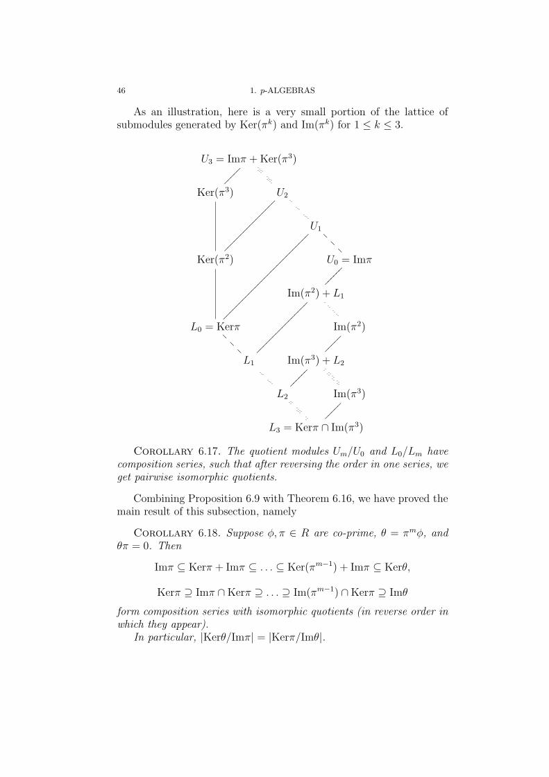
46 1. p-ALGEBRAS
As an illustration, here is a very small portion of the lattice ofsubmodules generated by Ker(πk) and Im(πk) for 1 ≤ k ≤ 3.
U3 = Imπ +Ker(π3)
U2
U1
??
?
U0 = Imπ
Ker(π3)
Im(π2) + L1
Im(π2)
Ker(π2)
Im(π3) + L2
Im(π3)
L0 = Kerπ
??
?
L1
L2
L3 = Kerπ ∩ Im(π3)
Corollary 6.17. The quotient modules Um/U0 and L0/Lm havecomposition series, such that after reversing the order in one series, weget pairwise isomorphic quotients.
Combining Proposition 6.9 with Theorem 6.16, we have proved themain result of this subsection, namely
Corollary 6.18. Suppose ϕ, π ∈ R are co-prime, θ = πmϕ, andθπ = 0. Then
Imπ ⊆ Kerπ + Imπ ⊆ . . . ⊆ Ker(πm−1) + Imπ ⊆ Kerθ,
Kerπ ⊇ Imπ ∩Kerπ ⊇ . . . ⊇ Im(πm−1) ∩Kerπ ⊇ Imθ
form composition series with isomorphic quotients (in reverse order inwhich they appear).
In particular, |Kerθ/Imπ| = |Kerπ/Imθ|.

6. HILBERT’S THEOREM 90 FOR pBr(K) 47
6.4. Hilbert’s Theorem 90 for pBr(K). Let K/F be a cyclicfield extension of degree n, with σ a generator of Gal(K/F ). We donot assume anything on charF .
Abelian groups of exponent p with a σ-action can be viewed asmodules over R = Zp[σ|σn = 1]. Let M be such a module. Later inthis subsection we specialize to M = pBr(K).
From now on, Σ = 1 + σ + · · · + σn−1 ∈ R is the trace element,so that left multiplication by Σ induces TrK/F : M → M . Also letπ = 1− σ, so that Σ · π = 0, and obviously Im(π) ⊆ Ker(Σ). Hilbert’stheorem 90 for M is precisely the statement Ker(Σ) = Im(π).
In this general setup, Theorem 6.1 has the following proof:
Proposition 6.19. If n is prime to p, then Hilbert’s theorem 90holds for M :
Ker(Σ) = (1− σ)M.
Proof. Σ, 1− σ are co-prime since the image n of Σ in R/⟨1− σ⟩is invertible. We are done by Lemma 6.4.
We now factor the trace element in R in the general case. Writen = [K :F ] = prd, where (p, d) = 1.
Proposition 6.20. Let π = 1−σ. The trace element Σ ∈ R factorsas Σ = πpr−1ϕ, where ϕ is coprime to π in R. Also Σ · π = 0.
Proof. That Σπ = σn − 1 = 0 is obvious. Work in the preimageR1 = Zp[λ] of R: 1− λn = (1− λd)p
r= (1− λ)p
r(1 + λ+ · · ·+ λd−1)p
r,
so that 1 + λ + · · · + λn−1 = (1 − λ)pr−1(1 + λ + · · · + λd−1)p
r. The
image in R is Σ = πpr−1(1 + σ + · · ·+ σd−1)pr.
As before, ϕ = (1+σ+ · · ·+σd−1)pris coprime to π since the image
dprin R/⟨π⟩ = Zp is invertible. We define the ’Hilbert defect’ of the R-module M as a measure of
how badly does Hilbert’s theorem 90 fail for M :
DH(M) = Ker(Σ)/Im(π).
The dual quotient (cf. Corollary 6.18) is Ker(π)/Im(Σ). The kernel ofπ = 1− σ is simply the invariant subgroup Mσ. We define the ’Galoisdefect’ as the quotient
DG(M) =Mσ/Im(Σ).
Now apply Corollary 6.18 to get filtrations of DH(K/F ) and DG(K/F ).Recall that n = [K :F ] = prd where (p, d) = 1, and set m = pr − 1. Asin subsection 6.3, let
Lk = πk(M) ∩Mσ,
48 1. p-ALGEBRAS
Uk = Ker(πk) + πM
ThenMσ = L0 ⊇ L1 ⊇ . . . ⊇ Lm = Im(Σ),
πM = U0 ⊆ U1 ⊆ . . . ⊆ Um = Ker(Σ),
where the equalities in the right come from Proposition 6.9. Checkthat DH(M) = Um/U0, while DG(M) = L0/Lm.
By Theorem 6.16, the quotients are isomorphic after reversing or-der: Uk/Uk−1∼=Lk−1/Lk (1 ≤ k ≤ m).
Corollary 6.21. DH(M) and DG(M) have decomposition serieswith isomorphic quotients after reversing order in one of them.
In particular, DH = 1 iff DG = 1.
If [K :F ] is prime to p, then by Proposition 6.19, DH(M) = 1 andDG(M) = 1. On the other extent we have that if n = [K :F ] = pr, thenπn = 0 and Im(πn−k) ⊆ Ker(πk) always holds, so by Corollary 6.3 wehave that DH(M) and DG(M) vanish iff Ker(πk) = Im(πn−k) for some0 < k < n.
Remark 6.22. If p = 2 and n = [K :F ] = 2, then DH(M) = DG(M)since π = TrK/F (and the above filtration has only one level).
Example 6.23. A possible application of the above results is for themodule M = pBr(K). Note that Br(K) is a module over Z[σ|σn = 1](where σ acts on Br(K) by the action on the base field, and Z acts byexponentiation). The kernel of p ∈ Z[σ] is the subgroup of classes ofexponent dividing p, i.e. M = pBr(K). As required, this is a moduleover R = Zp[σ|σn = 1].
In the special case M = pBr(K) we write DH(K/F ) instead ofDH(pBr(K)), and similarly for DG.
Corollary 6.21 gives corresponding filtrations for the quotients
DH(K/F ) = Ker(TrK/F )/πpBr(K)
andDG(K/F ) = pBr(K)σ/Im(TrK/F ).
DG(K/F ) can be given a new form if charF = p.
Remark 6.24. If charF = p, then corK/F : pBr(K) → pBr(F ) isonto by Corollary 5.12. Thus Im(TrK/F ) = Im(resF→K corK/F ) =Im(resF→K), and this group is denoted by [F, F ⊆ K2(K) = [K,F(the last equality is Theorem 5.6).
In this case
DH(K/F ) = Ker(TrK/F )/[F, F.

6. HILBERT’S THEOREM 90 FOR pBr(K) 49
We can show that very frequently DG, and thus also DH, are non-trivial. Recall that for an extension F1/F , Br(F1/F ) denotes the kernelof resF→[1
/F ] : Br(F ) → Br(F1), that is, the subgroup of Br(F ) con-sisting of algebras split by F1.
Theorem 6.25. Assume charF = p. Let K/F be a cyclic ex-tension, and F ⊂ F1 ⊆ K the subfield of dimension p over F . IfBr(F1/F ) = 1, then DG(K/F ) = 1, that is, the map
resF→K : pBr(F ) → pBr(K)σ
is not onto.
By Corollary 6.21, we also have DH(K/F ) = 1, so that Hilbert’stheorem 90 fails in this case. We need two lemmas before a proof ofthe theorem is given.
Lemma 6.26. Let A ∈ Br(K). For all the algebras B over F withresF→KB = A, the number lcmexp(B), [K :F ] is a constant.
Proof. Let n = [K :F ]. Suppose the algebras B1, B2 over F havethe same restriction to K. Then B′ = B2⊗B1
op is split by K, so that
exp(B2) = exp(B1⊗B′) | lcmexp(B1), exp(B′) | lcmexp(B1), n,
and alsolcmexp(B2), n | lcmexp(B1), n.
Note that the same result holds with exp(Br(K/F )) instead of
[K :F ].
Lemma 6.27. Let L/F be a cyclic extension of degree pt+1 withGal(L/F ) = ⟨σ⟩, and let b ∈ F . Set F1 = Lσp
, an intermediate subfieldof dimension p over F . Then the cyclic algebra C = (L/F, σ, b) satisfies
C⊗pt ∼ (F1/F, σ, b).
Proof. Let ω = (α0, . . . , αt) denote the Witt vector (over F ) cor-responding to L, so that C = [ω, b) — a symbol p-algebra of degreept+1 (see [20] for some basic properties of such symbols). Then
C⊗pt
= [(α0, . . . , αt), b)⊗pt
∼ [pt(α0, . . . , αt), b)
= [(0, . . . , 0, α0), b)
∼ [α0, b),
the last symbol is of degree p over F , and contains F1 = F [x|xp − x =α0].
50 1. p-ALGEBRAS
Proof of Theorem 6.25. Let K1 be a subfield of K such that[K :K1] is prime to p, and n1 = [K1 :F ] is a power of p. Then F ⊂F1 ⊆ K1 ⊆ K.
Let L/K1 be an extension of dimension p over K1, which is cyclicover F (such an extension always exist, by Corollary 1.29). Let σ bea generator of Gal(L/F ). Pick some 1 = u ∈ Br(F1/F ), then u is theclass of an algebra containing F1 as a maximal subfield, which is thusof the form (F1/F, σ, b) for some b ∈ F .
Consider the cyclic algebra C = (L/F, σ, b). By Lemma 6.27,C⊗n1 ∼ (F1/F, σ, b) which is non split by the choice of b. Thusexp(C) = pn1.
Let A = resF→KC. Since C contains K1 as a subfield and is ofdegree pn1, we have that exp(A) | ind(A) divides p, and so [A] ∈ pBr(K),and is obviously invariant. Let B ∈ Br(F ) such that resF→KB = A. ByLemma 6.26, we have that n1p = exp(C) divides (exp(C), [K :F ]) =(exp(B), [K :F ]), but since n1p does not divide [K :F ], we see thatexp(B) cannot divide [K :F ], and so cannot be equal to p.
Thus A is not a restriction from pBr(F ), as asserted.
We now move into a more complicated setting. The results belowcan be formulated for general modules of exponent p, but we prefer tospecialize to charF = p and M = K2(K).
The fact that Σ is a power of π when n = pr enables us to go alittle deeper in that case. Let F ⊆ L ⊆ K be an intermediate field,where [L :F ] = n1 and [K :L] = n2 are powers of p. As before π = 1−σwhere Gal(K/F ) = ⟨σ⟩, so that Gal(K/L) = ⟨σn2⟩.
Agree that [L, F ⊆ K2(K) denotes the image of resL→K : K2(L) →K2(K) (this is a different object than K2(L)). DH(L/F ) is a quotientof submodules of K2(L). We can generalize it to measure the quotientof submodules of [L, F ⊆ K2(K), by defining
DH(K,L/F ) = u ∈ [L, F : TrL/Fu = 0/π[L, F,so that the usual Hilbert defect is DH(K/F ) = DH(K,K/F ).
Theorem 6.28. If [K :F ] is a p power and F ⊆ L ⊆ K, then
DH(K,L/F ) =Ker(TrL/F )
π[L, F∼=
Ker(TrK/F )
Ker(TrL/F ) + π[K,F.
In particular, DH(K,L/F ) is a quotient of DH(K/F ).
Proof. Similarly to the definition of Uk, we set
Vk = v ∈ [L, F : πkv = 0+ π[L, F.
6. HILBERT’S THEOREM 90 FOR pBr(K) 51
Since n2 = [K :L] is a p power, ΣK/L = 1 + σn1 + · · ·+ σn1(n2−1) =(1 − σn1)n2−1. But n1 is a p power too, so that (1 − σn1) = (1 − σ)n1
and ΣK/L = πn1(n2−1). Thus multiplication by πn1(n2−1) induces the thetrace map TrK/L from K2(K), onto [L, F.
It follows that ΣK/L ·Un1(n2−1)+k = Vk for 0 ≤ k < n1. Fortunately,Ker(ΣK/L) ⊆ Un1(n2−1) by definition of Un1(n2−1), so that multiplicationby ΣK/L maps
Un1n2−1/Un1(n2−1) = Ker(TrK/F )/(KerK/L + π[K,F)
(a quotient of DH(K/F ) = Ker(TrK/F )/π[K,F) bijectively to
Vn1−1/V0 = Ker(TrL/F )/π[L, F = DH(K,L/F ).
For the dual (and much easier) result on DG, define DG(K,L/F ) tobe the Galois defect of [L, F over [F, F inside K2(K):
DG(K,L/F ) = [L, Fσ/[F, F.
Proposition 6.29. DG(K,L/F ) is a submodule of DG(K/F ).
Proof. By definition
DG(K,L/F ) = [L, Fσ/[F, F ⊆ [K,Fσ/[F, F.
Note that in the decomposition series of length n− 1 of DH(K/F ),the upper n1 − 1 components correspond to DH(K,L/F ). Likewise, inthe decomposition of DG(K/F ) to isomorphic (in reverse order) quo-tients, the lower n1 − 1 components belong to DG(K,L/F ).
We end this subsection with a description of DH(K,K/L) in thespecial case [K :L] = [L :F ] = 2, p = 2. Letting π = 1 − σ, we havethat π4 = 0, TrK/F = 1 + σ + σ2 + σ3 = π3, TrL/F = π, and TrK/L =1 − σ2 = π2. The (modular) lattice generated by the submodulesKer(π) ⊆ Ker(π2) ⊆ Ker(π3) and Im(π3) ⊆ Im(π2) ⊆ Im(π) of K2(K)is similar to that of page 46:
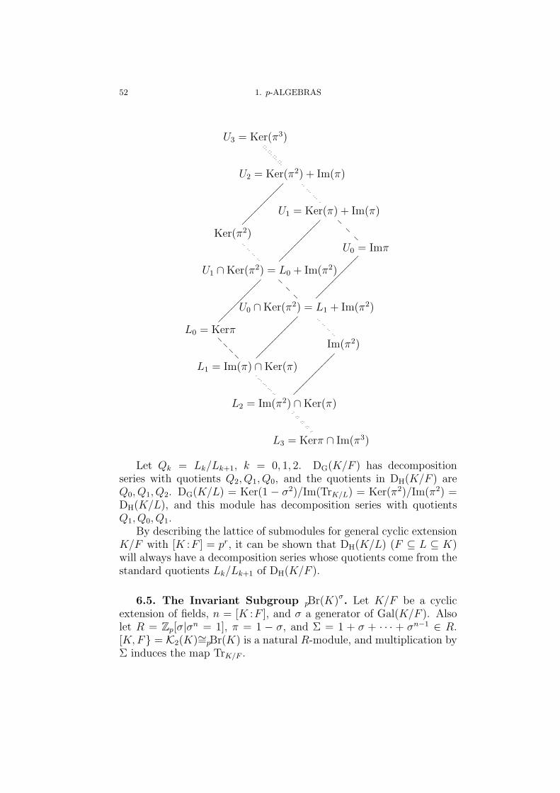
52 1. p-ALGEBRAS
U3 = Ker(π3)
U2 = Ker(π2) + Im(π)
U1 = Ker(π) + Im(π)
??
?
U0 = Imπ
Ker(π2)
U1 ∩Ker(π2) = L0 + Im(π2)
??
?
U0 ∩Ker(π2) = L1 + Im(π2)
Im(π2)
L0 = Kerπ
??
??
L1 = Im(π) ∩Ker(π)
L2 = Im(π2) ∩Ker(π)
L3 = Kerπ ∩ Im(π3)
Let Qk = Lk/Lk+1, k = 0, 1, 2. DG(K/F ) has decompositionseries with quotients Q2, Q1, Q0, and the quotients in DH(K/F ) areQ0, Q1, Q2. DG(K/L) = Ker(1 − σ2)/Im(TrK/L) = Ker(π2)/Im(π2) =DH(K/L), and this module has decomposition series with quotientsQ1, Q0, Q1.
By describing the lattice of submodules for general cyclic extensionK/F with [K :F ] = pr, it can be shown that DH(K/L) (F ⊆ L ⊆ K)will always have a decomposition series whose quotients come from thestandard quotients Lk/Lk+1 of DH(K/F ).
6.5. The Invariant Subgroup pBr(K)σ. Let K/F be a cyclicextension of fields, n = [K :F ], and σ a generator of Gal(K/F ). Alsolet R = Zp[σ|σn = 1], π = 1 − σ, and Σ = 1 + σ + · · · + σn−1 ∈ R.[K,F = K2(K)∼=pBr(K) is a natural R-module, and multiplication byΣ induces the map TrK/F .

6. HILBERT’S THEOREM 90 FOR pBr(K) 53
As seen in the last subsection (Corollary 6.21), the R-module
DH(K/F ) = Ker(TrK/F )/π[K,Fwhich measures the failure of Hilbert’s theorem 90 for K2(K)∼=pBr(K)has a composition series which, after reversing the order of quotients,is the same as that of DG(K/F ) = K2(K)σ/[F, F.
In this subsection we study the invariant subgroup pBr(K)σ =K2(K)σ. We describe a special subgroup of K2(K)σ, and study somegeneric examples.
It was proved by Eilenberg-MacLane [11] that for every Galois ex-tension K/F (regardless of charF ), the quotient Br(K)σ/Im(resF→K)embeds into H3(Gal(K,F ), K∗). If K/F is cyclic then H3 = 1, and soevery invariant class in Br(K) is a restriction from Br(F ). It should beemphasized that the relation to the relative invariant groups nBr(K)is not too tight: the fact that an invariant [A] ∈ nBr(K) is a restric-tion, does not show that it is a restriction from nBr(F ). In generalA = resF→KB with exp(A) | exp(B), and, in view of Theorem 6.25, oneshould not expect to have an equality.
The situation in prime-to-p extensions do not reflect the generalcase:
Proposition 6.30. If n = [K :F ] is prime to p, then K2(K)σ =[F, F.
Proof. By Theorem 6.1 we have that DH(K/F ) = 1, so thatDG(K/F ) = 1 too.
Recall that HK/F = a ∈ K : σ(a)− a ∈ ℘(K) (Subsection 1.3),where ℘(K) = αp − α : α ∈ K. HK/F/(F + ℘(K))∼=Zp if p dividesn (Theorem 1.23), and HK/F = F + ℘(K) otherwise (Corollary 1.18).We assume that p divides [K :F ].
Proposition 6.31. We have that [HK/F , F ⊆ K2(K)σ. Also, ev-ery class of [HK/F , F/[F, F has a representative which is one symbol.
Proof. Let a ∈ HK/F , β ∈ F . Then σ(a) − a = ℘(k) for somek ∈ K, and σ([a, β)) = [a+ ℘(k), β) = [a, β).
Recall that there is some a0 ∈ K such that HK/F = F+℘(K)+Zpa0(Proposition 1.23). Thus for every a ∈ HK/F , we have that a = ja0 +℘(k) + α for some j ∈ Zp, k ∈ K and α ∈ F , so for every β ∈ Fwe can write [a, β = [ja0 + α, β ≡ [a0, β
j mod [F, F. Sum of suchsymbols can thus be given the same form.
From the proof it follows that the map β 7→ [a0, β + [F, F fromF ∗ to [HK/F , F is onto, so that [HK/F , F/[F, F is a quotient groupof F ∗.

54 1. p-ALGEBRAS
Remark 6.32. By Corollary 1.15, if a ∈ HK/F , then for everyx ∈ [a, β) such that xp − x = a, we have that K[x] is Galois over F .
By Theorem 5.6, pBr(K) is generated by the symbol algebras [a, β)where a ∈ K, β ∈ F . We now study an invariant algebra of this form.Again we emphasize that by the Eilenberg-MacLane result, [a, β) isthe restriction of some algebra B over F , which has exponent boundedby p[K :F ]. Essentially we ask if it is a restriction of an algebra ofexponent p (or even better — of index p).
Let a ∈ K, β ∈ F , and R = [a, β) ∈ pBr(K)σ.Let x, y be a SCOG (Definition 4.1) of [a, β), and u′, y′ a SCOG
of [σ(a), β). We may assume this is the same algebra, so that u′, y′ ∈[a, β). Now, F [y]∼=F [y′], so there is a conjugation that carries y′ toy; let u be the image of u′ under this conjugation. Now extend σ(the generator of Gal(K/F )) to an automorphism of R, by σ(x) = uand σ(y) = y (this can be done since the defining relations xp − x =a, yp = β and yxy−1 = x + 1, are preserved). In this context it isworth mentioning that a central simple algebra over F is invariant iffthe automorphisms of K over F can be extended to automorphisms ofA ([10, Section 23, (12)]).
We assume henceforth that p |n = [K :F ].
Proposition 6.33. Suppose a ∈ ℘(K) (otherwise [a, β) is split),and let x, y, u ∈ R be as above.
If σn(x) ∈ K[x], then [a, β ∈ [HK/F , F (moreover, we can write[a, β = [α, β for α ∈ HK/F ).
Proof. From Lemma 4.8 it follows that u = σ(x) = x+γ0+γ1y+· · ·+ γp−1y
p−1 for γi ∈ K. Now compute that σn(x) = x+ trK/F (γ0) +· · · + trK/F (γp−1)y
p−1, but since σn acts trivially on K, we have thatσn(x) satisfies ℘(σn(x)) = σn(℘(x)) = a = ℘(x). By the assumptionσn(x) and x commute, so that ℘(σn(x) − x) = 0 and it follows thatσn(x) = x+j for some j ∈ Zp. Thus trK/F (γi) = 0 for every i > 0. Usethis to write γi = δi − σδi (i > 0), and let z = x + δ0 + · · · + δp−1y
p−1
(δ0 ∈ K can be arbitrary).Compute that σ(z) = z+(γ0+σδ0−δ0). (If j = 0, z could be made
an element of Rσ). Set α = ℘(z) = a+ δp0 − δ0 + δp1β + · · ·+ δpp−1βp−1,
and compute that σ(α)− α = ℘(γ0 + σδ0 − δ0). Thus α ∈ HK/F .Since z, y form a SCOG of [α, β), we are done.
Remark 6.34. If, in the above setting, σn(x) = x, then [a, β =[α, β for α ∈ F . In particular, [a, β)K = [α, β)F⊗FK.
6. HILBERT’S THEOREM 90 FOR pBr(K) 55
Proof. In the above computations, we have j = σn(x)−x = 0, sothat trK/F (γ0) = 0 and we can choose δ0 ∈ K such that σ(α) = α andα ∈ F . This completes the proof.
The fact that σ extends to an automorphism of R of the same or-der, enables us to give another proof. The invariant subalgebra Rσ
is an F -subalgebra of R, such that R∼=Rσ⊗FK [30, 7.2.14]. Count-ing dimensions, deg(Rσ/F ) = p. Since y ∈ Rσ satisfies yp ∈ F , wecan apply Albert’s Theorem [1, VII.24], and find some z ∈ Rσ suchthat α = zp − z ∈ F , yz = zy + y. Then Rσ∼=[α, β)F and we have[a, β)∼=[α, β)F⊗FK = [α, β)K .
We illustrate the method in the last remark by an example.
Example 6.35. Let k be a field of characteristic 2, λ1, λ2 transcen-dental over k, K = k(λ1, λ2), σ : K → K the automorphism definedby σ : λ1 ↔ λ2, and F = Kσ.
Then r = [λ1, λ1 + λ2 is σ-invariant, for [λ1, λ1 + λ2 = [λ2, λ1 + λ2.Taking a SCOG x, y for R = [λ1, λ1 + λ2) (so that x2 − x = λ1, y
2 =λ1+λ2 and yxy
−1 = x+1), we look for u ∈ R such that yuy−1 = u+1and u2−u = λ2. Writing u = x+γ0+γ1y, it is easy to guess u = x+y.
Then σ is extended to an automorphism of R by σ : x 7→ u, y 7→y, so we compute that σ2(x) = σ(u) = x. Applying the zero-trace
argument of Remark 6.34, we find out that λ1 =λ1λ2
λ1+λ2+(
λ1
λ1+λ2
)2(λ1+
λ2), so that
[λ1, λ1 + λ2 = [λ1λ2λ1 + λ2
, λ1 + λ2 ∈ [F, F.
Note that in this example Gal(K[x]/F ) = Z22 (by Theorem 1.19, as
x2 − x ∈ F + ℘(K)).
The next example is generic for [HK/F , F, and we suspect it doesnot belong to [F, F.
Example 6.36 (A generic element of [HK/F , F). Let k be a field ofcharacteristic 2, µ, η transcendental variables over k, and K = k(µ, η).Define σ ∈ Aut(K) by σ : µ 7→ µ+ 1, σ : η 7→ η, and let F = Kσ.
Let a = µ2(1 − µ). Then a ∈ HK/F , since σ(a) − a = ℘(µ). Andindeed, r = [a, η is invariant: σ(r)− r = [σ(a)− a, η = [µ− µ2, η =0.
Note that a ∈ F +℘(K) (for tr(µ) = 1, cf. Theorem 1.23). Thus ifx ∈ [a, η) satisfies x2 − x = a, then Gal(K[x]/F )∼=Z4.
56 1. p-ALGEBRAS
6.6. Remarks on Corestriction. We make some remarks on thecorestriction in Brauer groups for cyclic extensions, and use them toshow that Hilbert’s theorem 90 does fail for the Brauer groups.
Proposition 6.37. Let K/F be a cyclic extension of odd dimensionn, such that F has n-roots of unity.
Then corK/F : nBr(K) → nBr(F ) is onto Br(K/F ).
Proof. Let u ∈ Br(F ) be a class split by K, then some algebraA ∈ u has K as a maximal subfield. Writing K = F [α|αn = a], wesee that A is a cyclic algebra A = (a, b)n;F for some b ∈ F . The cyclicalgebra (α, b)n;K over K satisfies corK/F (α, b)n;K = (Nσ(α), b)n;F =((−1)n−1a, b)n;F = (a, b)n;F .
If [K :F ] = 2 and K/F is generated by α =√1 + t2 for some t ∈ F ,
then a = α2 = NK/F (α2+tα) is a norm, so that corK/F covers Br(K/F )
by the same argument.However, this result is not true for [K :F ] = 2 in general:
Example 6.38. The class of the standard quaternions [H] ∈ Br(C/R)is not a corestriction from Br(C) = 1.
More can be said if Br(K) = 1.
Corollary 6.39. Let K/F be a (solvable) Galois extension of odddimension n = [K :F ]. Suppose F has n-roots of unity.
If Br(K) = 1, then Br(F ) = 1.
Proof. By induction we may assume K/F is cyclic.Let u ∈ Br(F ), then resF→K(u) ∈ Br(K) = 1, so that u ∈ Br(K/F ).
By the proposition, u is a corestriction from Br(K) = 1, so thatu = [F ].
Note that if F0 ⊆ F , then Br(F0) = Br(F/F0) since Br(F ) = 1.Here is a diagram of the groups involved in the next setting.
Br(K)
corK/F
TrK/F
%%JJJJ
JJJJ
J
0 // Br(K/F ) // Br(F )resF→K// Br(K)σ
Proposition 6.40. Let K/F be a cyclic extension of odd dimensionn, Gal(K/F ) = ⟨σ⟩, such that F has n-roots of unity.
If Br(K/F ) = 1 then Hilbert’s theorem 90 does not hold for nBr(K)over nBr(F ), that is, there are u ∈ nBr(K) with zero trace (whereTrK/F = resF→K corK/F ), which are not of the form u = (1 − σ)vfor any v ∈ Br(K).

6. HILBERT’S THEOREM 90 FOR pBr(K) 57
Proof. Let 1 = [A] ∈ Br(F ) be split by K. By proposition 6.37one can write [A] = [corK/F (A1)]. Then
TrK/F ([A1]) = resF→KcorK/F [A1] = resF→K [A] = 0.
Assuming Hilbert’s theorem 90 holds, we can write [A1] = (1− σ)[A2]for some [A2] ∈ Br(K); but then
[A] = [corK/F (A1)] = [corK/F (A2)]− [corK/F (σA2)] = 0,
a contradiction. Suppose charF = 0 and F has all the roots of unity. By Merkurjev-
Suslin theorem, nBr(K)∼=K2(K)/nK2(K). Let u denote an elementin K2(K) corresponding to [A] of the proposition; we have chosen Asuch that TrK/F (u) ≡ 0 in the relative K2 group, that is TrK/F (u) ∈nK2(K). As we have seen, it does not follow that u ≡ (1 − σ)v(mod nK2(K)) for some v ∈ K2(K).


CHAPTER 2
Brauer Algebras
1. Introduction
Let p be a prime number, F a field with char(F ) = p. Building onAmitsur’s famous example [2], Saltman [34] proved that the genericdivision algebra of degree pν and exponent pµ is not a crossed productwith respect to any group for ν ≥ µ ≥ 3 (µ = 2 for p an odd prime,if F has no p-roots of unity). The situation for exponent p and degreepν , ν ≥ 3, remained open (except for degree 8 and exponent 2, whereit is a crossed product with respect to Z2 × Z2 × Z2, [29]).
In this chapter we study Brauer algebras of degree pν and exponentp, making several reductions on possible sets of generators of a Zν
p-Galois extensions of the center.
The base fields in the examples we study contain finitely many rootsof unity of p-power order. Using the ultraproduct argument at the endof [33], it is possible to produce an algebra with similar properties,such that the center contains the whole group µp∞ .
Once one produces a central simple algebra of the required degreeand exponent which is not a Zν
p-crossed product, the generic divisionalgebra would be a noncrossed product, for it is known that the genericdivision algebra of degree pν and arbitrary exponent is not a crossedproduct with respect to any other group. An example was presentedin [27] and [30], but there were several major gaps. We continue theinvestigation of this example in a more general situation described in§4, closing some of the gaps. One gap remains, so the problem ofproducing a noncrossed product of exponent p is still open.
2. The Leading Monomial Technique
The technique of the leading monomial enables one to pass fromgood elements of a generic algebra to homogeneous good elements of amore concrete algebra. This was used numerous times, for example [3]or [33].
Let M be a commutative linearly ordered monoid, and T an M-graded ring without zero divisors: T = ⊕α∈MTα, with TαTβ ⊆ Tα+β.
59
60 2. BRAUER ALGEBRAS
Let Φ = ϕ be a set of grading-preserving automorphisms of T(that is ϕ(Tα) ⊆ Tα for all ϕ ∈ Φ, α ∈ M), such that the fixed subringTΦ ⊆ Cent(T ).
For any element r =∑rα ∈ T , the upper component of r is µ(r) =
rα0 , where α0 is maximal in α : rα = 0.Remark 2.1. a. If f ∈ TΦ and fg ∈ TΦ, then g ∈ TΦ.b. µ(fg) = µ(f)µ(g).c. If f ∈ TΦ then µ(f) ∈ TΦ.d. If f, g commute in T , then so do µ(f), µ(g).
Let θ > 1 be an integer, θ = 0 in T . An element f ∈ T is θ-invariantif f θ ∈ TΦ, but f i ∈ TΦ for any 0 < i < θ.
Proposition 2.2. If f ∈ T is θ-invariant, then so is µ(f).
Proof. µ(f)θ = µ(f θ) is invariant since f θ is.We first show that if f is θ-invariant then µ(f) ∈ TΦ. Write f =
g + z where z is the sum of the invariant components in f , and g thesum of noninvariant components. In particular z ∈ Cent(T ), so thatz, g commute. By assumption, g = 0.
Assume µ(f) is a summand in z. The upper component of f θ−zθ =(g + z)θ − zθ = θzθ−1g + · · ·+ gθ is the upper component of θzt−1g, sothat µ(θzθ−1g) = θµ(z)θ−1µ(g) is invariant. Now µ(g) is invariant forµ(z) is, a contradiction to the definition of g.
Finally, suppose µ(f)i ∈ TΦ, then replacing i with (i, θ) we mayassume i | θ, and f i is θ/i-invariant. By what we have just proved,µ(f i) ∈ TΦ unless θ/i = 1, so that i = θ.
We call f1, . . . , fν a θ-set if f1, . . . , fν are pairwise commuting,f θi ∈ TΦ, and f i1
1 · · · f iνν ∈ TΦ for all 0 ≤ i1, . . . , iν < θ, unless i1 =
· · · = iν = 0. Note that if f belongs to a θ-set then f is θ-invariant. IfTΦ is a field containing θ-roots of unity, then a θ-set is a standard setof generators for a Zν
θ -Galois field extension of TΦ.
Proposition 2.3. If the set f1, . . . , fν is a θ-set, then so is theset µ(f1), . . . , µ(fν).
Proof. In general, f i11 · · · f iν
ν ∈ TΦ iff every ij ≡ 0 (mod θ).Suppose µ(f1)
i1 · · ·µ(fν)iν = µ(f i11 · · · f iν
ν ) ∈ TΦ, then f i11 · · · f iν
ν
cannot be θ-invariant by the previous proposition, so that i1 ≡ · · · ≡iν ≡ 0 (mod θ).
Let ρθ denote a (fixed) θ-root of unity in T .
Proposition 2.4. Let f1, . . . , fν be a θ-set, and g a θ-invariantelement such that for every i = 1, . . . , ν, gfig
−1 = ραiθ fi. Assume θ is

3. THE GENERIC ELEMENTS CONSTRUCTION 61
a power of some prime p. Then T has a θ-set of the same size, with gas one of its elements.
Proof. Case 1: f1, . . . , fν commute with g. The intersection ofthe subalgebras Li = TΦ[f1, . . . , fi−1, fi+1, . . . , fν ], i = 1, . . . , ν, is TΦ,so that for some i we have gθ/p ∈ Li. Then f1, . . . , fi−1, fi+1, . . . , fν , gform a θ-set of size ν, as asserted.
Case 2: Not every fi commute with g; for example assume αν = 0.
Then fi = f−1i fαi/αν (mod θ)ν , i = 1, . . . , ν − 1, commute with g. Since
L = TΦ[f1, . . . , ˜fν−1] ⊂ TΦ[f1, . . . , fν ], g does not belong to L (for
otherwise fν , g would commute). Thus, f1, . . . , ˜fν−1, g form a θ-set.
3. The Generic Elements Construction
We apply the leading monomial technique to an important specialcase.
Let R = (K/F, σ, b) be a cyclic algebra of degree n and exponentθ, and let z ∈ R be an element such that
(∀k ∈ K)zkz−1 = σ(k), zn = b.
Let λ be an indeterminate over K, and extend σ to K(λ) by as-signing σ(λ) = λ. R = R⊗F F (λ) = K(λ)[z] = (K(λ)/F (λ), σ, b) is ofcourse cyclic of the same degree and exponent asR. The idea is to mix λwith elements of R: take K = K(λθ) and R = K(λθ)[λz] ⊆ R. Alsolet F = Cent(R) = F (λθ). Note that R ∼= (K(λθ)/F (λθ), σ, λnb) isagain cyclic of degree n.
Theorem 3.1. exp(R) = θ.
Proof. ByWedderburn’s criterion, bθ ∈ NK/F (K), but bi ∈ NK/F (K)for any 0 < i < θ.
We apply the same criterion for λnb in the extension K(λθ)/F (λθ).Write bθ = NK/F (β), thenNK(λθ)/F (λθ)(λ
θβ) = (λnb)θ, so that exp(R) ≤θ. On the other hand, suppose (λnb)i = NK(λθ)/F (λθ)(f/g) where
f, g ∈ K[λθ], 0 ≤ i < θ. Multiplying by NK(λθ)/F (λθ)(g) and comparingdegrees of λ, we see that nθ |ni, so that i = 0.
Note that R is the ring of central quotients of T = K[λθ][λz],which is N-graded as a ring of polynomials in λ. Let k ∈ K be agenerator of K/F . Conjugation by z or by k induce grading-preservingautomorphisms, and the invariant subring under the conjugations isF.
Note that for any f ∈ K[λθ][λz] ⊆ R, µ(f) ∈ K[zθ]zα ·λu for some0 ≤ α < θ.
62 2. BRAUER ALGEBRAS
Suppose F contains θ-root of unity, denoted by ρθ. Let k1 be agenerator for the field extension Kσθ
/F , such that σ(k1) = ρθk1. Inparticular, kθ1 ∈ F .
Note that K[zθ] is the centralizer of k1 in R.
Lemma 3.2 (Going down R → R). If R contains a θ-set of size ν,then R has a θ-set f1, . . . , fν such that f1 = k1 and f2, . . . , fν ∈ K[zθ].
Proof. Let g1, . . . , gν ∈ R be a θ-set. Multiplying by centralelements, we may assume gi ∈ K[λθ][λz]. The leading monomials ofg1, . . . , gν (relatively to λ) form a θ-set by Proposition 2.3. We can thusassume gi ∈ K[zθ] · (λz)αi ⊆ R. Moreover, dropping the appropriatepowers of λ we have a θ-set f1, . . . , fν ∈ R, fi ∈ K[zθ] · zαi .
But now conjugation by k1 multiplies each fi by ραiθ , so we can
apply Proposition 2.4.
Remark 3.3 (Going up R → R). If f1, . . . , fν is a θ-set in R, suchthat k1 = f1, then it is a θ-set in R too.
Proof. Since fi commute with k1, we have that f2, . . . , fν ∈ CR(k1) =
K[zθ]. Now fi =∑n/θ−1
j=0 k(j)i zjθ =
∑n/θ−1j=0 (k
(j)i λ−jθ)(λz)jθ ∈ K(λθ)[λz] =
R.
4. Brauer’s Example
We now focus on the Brauer algebra.Recall the definition, following the notation in [30, Chap 7.3]. Fix
a prime number p, and let t, θ be powers of p. Denote by ρθ a primitiveθ-root of unity (over Q), and let µ0, ..., µt−1 be indeterminates overQ[ρθ]. The field Eθ,t = Q[ρθ](µ0, ..., µt−1) has an automorphism σ oforder t defined by σ : µi 7→ µi+1(mod t), σ : ρθ 7→ ρθ.
For any divisor n of t, let Kθ,n,t be the fixed subfield of Eθ,t underσn. The generalized Brauer example is the cyclic algebra Rθ,n,t =(Kθ,n,t/Kθ,1,t, σ, ρθ), of degree n over its center Kθ,1,t = Eσ
θ,t. In whatfollows we work with subalgebras of Rθ,t,t. Picking an element z ∈ Rθ,t,t
such that conjugation by z induce σ on Eθ,t and zt = ρθ, we can write
Rθ,t,t = Eθ,t[z].Note that zn commutes withKθ,n,t, so thatKn = Kθ,n,t[z
n] is a field.This is a maximal subfield of Rθ,t,t, of dimension t over the center F .Moreover, (zn)t/n = ρθ so that zn is a θt/n-root of unity in Kn, and wesometimes denote ρθt/n = zn. In particular, Kn
∼= Kθt/n,n,t.Let Rn = Kn[z], a cyclic algebra of degree n, with center Fn =
Kσn = Kθ,1,t[z
n] ∼= Kθt/n,1,t.
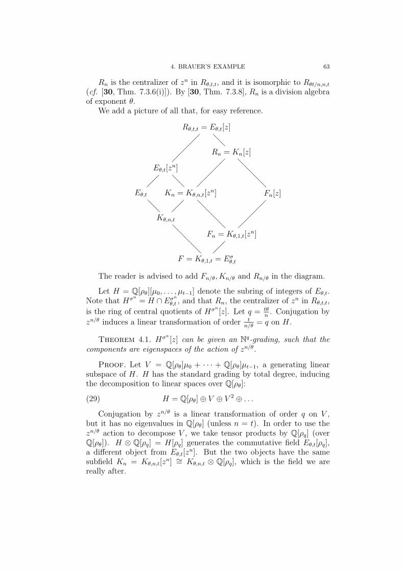
4. BRAUER’S EXAMPLE 63
Rn is the centralizer of zn in Rθ,t,t, and it is isomorphic to Rθt/n,n,t
(cf. [30, Thm. 7.3.6(i)]). By [30, Thm. 7.3.8], Rn is a division algebraof exponent θ.
We add a picture of all that, for easy reference.
Rθ,t,t = Eθ,t[z]
????
?
Rn = Kn[z]
????
????
????
Fn[z]
Eθ,t[zn]
????
?
Kn = Kθ,n,t[zn]
????
????
????
Fn = Kθ,1,t[zn]
Eθ,t
????
??
Kθ,n,t
????
????
????
F = Kθ,1,t = Eσθ,t
The reader is advised to add Fn/θ, Kn/θ and Rn/θ in the diagram.
Let H = Q[ρθ][µ0, . . . , µt−1] denote the subring of integers of Eθ,t.Note that Hσn
= H ∩ Eσn
θ,t , and that Rn, the centralizer of zn in Rθ,t,t,
is the ring of central quotients of Hσn[z]. Let q = tθ
n. Conjugation by
zn/θ induces a linear transformation of order tn/θ
= q on H.
Theorem 4.1. Hσn[z] can be given an Nq-grading, such that the
components are eigenspaces of the action of zn/θ.
Proof. Let V = Q[ρθ]µ0 + · · · + Q[ρθ]µt−1, a generating linearsubspace of H. H has the standard grading by total degree, inducingthe decomposition to linear spaces over Q[ρθ]:
(29) H = Q[ρθ]⊕ V ⊕ V 2 ⊕ . . .
Conjugation by zn/θ is a linear transformation of order q on V ,but it has no eigenvalues in Q[ρθ] (unless n = t). In order to use thezn/θ action to decompose V , we take tensor products by Q[ρq] (overQ[ρθ]). H ⊗ Q[ρq] = H[ρq] generates the commutative field Eθ,t[ρq],a different object from Eθ,t[z
n]. But the two objects have the samesubfield Kn = Kθ,n,t[z
n] ∼= Kθ,n,t ⊗ Q[ρq], which is the field we arereally after.
64 2. BRAUER ALGEBRAS
Over Q[ρq], we have the decomposition
(30) V = V0 ⊕ · · · ⊕ Vq−1,
where zn/θ acts on Vj as multiplication by ρjq.Substituting (30) in (29), we see that H[ρq] is a sum of all prod-
ucts V n00 · · ·V nq−1
q−1 . In order to see that this sum is direct, pick a basis
v(j)0 , . . . , v(j)n/θ−1 for Vj, then v(j)u 0≤j<q,0≤u<n/θ generateH (as a ring).
The transcendence degree of H is t, so that the v(j)u must be alge-braically independent. It is now obvious that every element is expressedin a unique way.
Let e0, . . . , eq−1 be the standard basis of Zq. The degree function
defined on monomials by v(j)u 7→ ej makes H[ρq] an Nq-graded ring,
with homogeneous components V n00 · · ·V nq−1
q−1 .Consider the ring H[ρq][u], subjected to the relations uhu−1 = σ(h)
(h ∈ H), un = ρq. It decomposes into a direct sum H[ρq][u] = H[ρq] +H[ρq] · u + · · · + H[ρq] · un−1. Since conjugation by u preserves thelinear components Vj, it preserves all the components, so that H[ρq][u]is (Nq × Zn)-graded. The same is true for the subalgebra Hσn
[ρq][u](and the only non-zero components are the products V n0
0 · · ·V nq−1
q−1 withn1 + 2n2 + · · ·+ (q − 1)nq−1 ≡ 0 (mod q/θ)).
Since Hσn[ρq] ∼= Hσn
[zn], we also have that Hσn[ρq][u] ∼= Hσn
[z],so that Hσn
[z] is (Nq × Zn)-graded. In particular, Hσn[z] is Nq-graded
with the components V n00 · · ·V nq−1
q−1 [z].
The reason we can’t use the same proof to decompose into eigenspacesof zn/k, k > θ, is that Hσn
[ρtk/n] ∼= Hσn[znθ/k]: the leftmost ring is com-
mutative, while the other is not.
Notation 4.2. From now on we assume θ = p. Also let n = pν,ν ≥ 2.
When ν = 2, Rn is a crossed product, as shown by the followingwell known fact (also see Example 1.1 in Chapter 3):
Remark 4.3. Let F be a field of characteristic = p, with p-rootsof unity. Any cyclic algebra R = (K/F, σ, b) = K[z] of degree p2 overF is a Zp × Zp-crossed product, by inspecting the subfield Kσp
[zp].
A final remark before we dive into the reductions: we have thechains of inclusions
Ft ⊂ · · · ⊂ Fn ⊂ Fn/p ⊂ · · · ⊂ F1,
Rt ⊃ · · · ⊃ Rn ⊃ Rn/p ⊃ · · · ⊃ R1,

4. BRAUER’S EXAMPLE 65
but the fields Kn (n = 1, p, p2, . . . , t) do not contain each other. Itfollows that the R
n = Kn(λp)[λz] do not satisfy any natural inclusion
relation among them.
Proposition 4.4. Suppose Rn has a p-set of size ν, then Rn has
a p-set of the same size, with k1, zn/p as two of the elements.
Proof. Recall that k1 is a generator of the extension Kp,p,t/Kp,1,t,such that σ(k1) = ρpk1. In particular, kp1 ∈ Kp,1,t. At the same time,Kσp
n = Fn[k1] and k1p ∈ Fn.
By Lemma 3.2, we have
Reduction 1. Rn contains a p-set f1, . . . , fν such that f1 = k1 andf2, . . . , fν ∈ Kn[z
p].
Reduction 2. We may assume that zn/pfiz−n/p = ραi
p fi for someαi.
Proof. Viewing fi as elements of Rp,t,t, we may multiply by suit-able central elements, and assume fi ∈ H[zp]∩Rn = Hσn
[zp] ⊂ Hσn[z].
We apply Theorem 4.1 to grade Hσn[z] with components which are
eigenspaces of zn/p. Note that we may choose k1 =∑t−1
i=0 ρ−ip µi ∈ V0,
so that f1 = k1 is homogeneous.Let kν be a generator of Kθ,n,t/Kθ,n/p,t, such that σn/p(kν) = ρpkν .
Since Rn = Fn[kν , z], central elements in Rn are exactly those invariantunder conjugation by z and kν . Moreover, since z, kν are eigenvectorsof zn/p, conjugation by them takes Vj (of the grading) to itself, and sois grading-preserving. This is enough to apply Proposition 2.3.
Replacing f1, f2, . . . , fν by their upper homogeneous parts, we stillhave a p-set, where every fi is an eigenvector of zn/p. Finally, since fiare p-central, the eigenvalues are powers of ρp, as required.
Reduction 3. We may assume that f2 = zn/p.
Proof. Note that f1 = k1 and zn/p commute.By the previous reduction fi are eigenvectors of zn/p, so we can
apply Proposition 2.4 with g = zn/p. This finishes the proof of Proposition 4.4. Corollary 4.5. Suppose ν ≥ 3. If R
n = Kn(λp)[λz] is a Zν
p-
crossed product, then Rn/p is a Zν−1
p -crossed product.
Proof. Suppose Rn has a p-set of size ν. By the last proposition,
Rn has a homogeneous p-set of the same size, with one of the elementsequals zn/p (and another equal k1).

66 2. BRAUER ALGEBRAS
Then CRn(zn/p) = Rn/p has a p-set of size ν − 1, and by Remark
3.3 so does Rn/p.
As already mentioned in Remark 4.3, Rp2 contains the p-set k1, z
p,
so we are led to study the next case, n = p3 (which we hope is not aZ3
p-crossed product for p = 2). This is done in Section 6.
Note that for p = 2, k1, z4, z2 + z−2 is a 2-set in R
8 .
5. Property D(p) for Algebras of Degree p2
A cyclic algebra R = (K/F, σ, b) = K[z|zkz−1 = σ(k), zn = b] ofdegree n is said to satisfy property D(f), f a divisor of n, if it decom-poses into a tensor product of cyclic subalgebras, one that containsKσf
and the other that contains F [zf ]. The property was introducedand studied in [33].
Suppose deg(R) = [K :F ] = p2, and that F contains a p-root ofunity. Choose a generator k1 for Kσp
/F such that kp1 ∈ F . Considerthe subfield L = F [k1, z
p], which is Z2p-Galois over F . We use square
brackets to denote the multiplicative commutator. By Skolem-Noether,there exist u, v ∈ R such that
(31) [u, k1] = 1, [u, zp] = ρp,
and
(32) [v, k1] = ρp, [v, zp] = 1.
Note that letting k2 be a cyclic generator for K/Kσp, u = k2 and
v = z is a solution to (31)+(32).We now add another constraint:
(33) [u, v] = 1.
Lemma 5.1. Property D(p) for R is equivalent to the existence ofa solution for (31)+(32)+(33).
Proof. Assume property D(p) is satisfied. Then there exist com-muting central simple subalgebras R1, R2 ⊂ R with R1 ∩ R2 = F ,R1R2 = R, k1 ∈ R1, z
p ∈ R2. We can thus find u ∈ R1 = CR(R2) suchthat [u, k1] = ρp and v ∈ R2 satisfying (32), and (33) is also clear.
Now suppose u, v commute, and satisfy (31),(32). We first showthat L[u, v] = R. Indeed, u ∈ L (for it does not commute with zp), sothat [L[u] :F ] ≥ p3. If L[u] = R, we are done. Otherwise, k1 is in thecenter of L[u], but does not commute with v — so that v ∈ L[u], andL[u, v] = R.
6. BRAUER’S EXAMPLE IN DEGREE n = p3 67
From (33) it now follows that up commutes with k1, zp, u, v, so that
up ∈ F . Similarly vp ∈ F , and F [k1, u], F [zp, v] are the commuting
subalgebras we are looking for.
We may look for a special kind of element: consider the constraint
(34) up ∈ F.
Proposition 5.2. If equations (31)+(34) has a solution, then sodo (31)+(32)+(33).
Proof. By the assumption, F [zp, u] is a (cyclic) central subalge-bra of R, of dimension p2. Its centralizer is of dimension p2, and con-tains the cyclic subfield F [k1]. Applying Skolem-Noether to this cen-tralizer we find v ∈ CR(F [z
p, u]) such that [v, k1] = ρp. u, v satisfy(31)+(32)+(33).
6. Brauer’s Example in Degree n = p3
Suppose Rp3 has a p-set of size 3. By Proposition 4.4, Rp3 has
the p-set zp2, k1, f3, where f3 ∈ Rp3 . Actually by the choice of f3 in
Reduction 2, f3 ∈ Hσp3
[zp].
Lemma 6.1. f3 does not commute with zp.
Proof. We draw a picture of the subalgebras of Rp3 appearing inthe sequel (this is a zoom into the rightmost square in the previousdiagram).
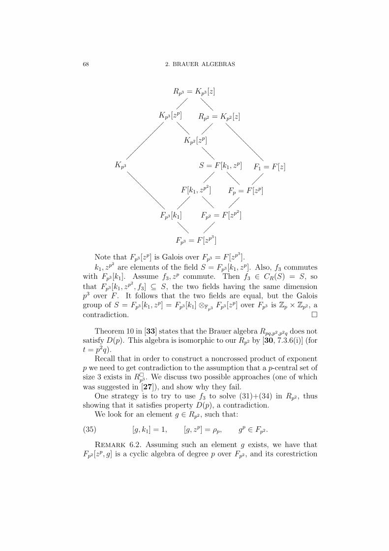
68 2. BRAUER ALGEBRAS
Rp3 = Kp3 [z]
????
??
Rp2 = Kp2 [z]
????
????
????
????
?
F1 = F [z]
Kp3 [zp]
????
??
Kp2 [zp]
????
??
S = F [k1, zp]
????
??
Fp = F [zp]
F [k1, zp2 ]
????
?
Fp2 = F [zp2]
Kp3
????
????
????
????
?
Fp3 [k1]
????
?
Fp3 = F [zp3]
Note that Fp3 [zp] is Galois over Fp3 = F [zp
3].
k1, zp2 are elements of the field S = Fp3 [k1, z
p]. Also, f3 commuteswith Fp3 [k1]. Assume f3, z
p commute. Then f3 ∈ CR(S) = S, so
that Fp3 [k1, zp2 , f3] ⊆ S, the two fields having the same dimension
p3 over F . It follows that the two fields are equal, but the Galoisgroup of S = Fp3 [k1, z
p] = Fp3 [k1] ⊗Fp3Fp3 [z
p] over Fp3 is Zp × Zp2 , a
contradiction.
Theorem 10 in [33] states that the Brauer algebra Rpq,p2,p2q does notsatisfy D(p). This algebra is isomorphic to our Rp2 by [30, 7.3.6(i)] (fort = p2q).
Recall that in order to construct a noncrossed product of exponentp we need to get contradiction to the assumption that a p-central set ofsize 3 exists in R
p3 . We discuss two possible approaches (one of which
was suggested in [27]), and show why they fail.One strategy is to try to use f3 to solve (31)+(34) in Rp2 , thus
showing that it satisfies property D(p), a contradiction.We look for an element g ∈ Rp2 , such that:
(35) [g, k1] = 1, [g, zp] = ρp, gp ∈ Fp2 .
Remark 6.2. Assuming such an element g exists, we have thatFp2 [z
p, g] is a cyclic algebra of degree p over Fp2 , and its corestriction

6. BRAUER’S EXAMPLE IN DEGREE n = p3 69
down the extension Fp2/Fp3 is
corFp2/Fp3(zp
2
, g) = (ρp, g).
Since f3 commutes with k1, zp2 , it belongs to Hσp2
[zp]. Apply the-
orem 4.1 with n = p2 to grade Hσp2
[z] ⊂ Rp2 with components whichare eigenspaces of zp.
It seems natural to continue as in Reduction 2, and replace f3 by aneigenvector of zp. Indeed, conjugation by z and by k2 (a cyclic generator
of Kσp2
p3 /Kσp
p3 ) preserve the grading (since z,k2 are eigenvectors of zp2),
so the p-power of an upper homogeneous component µ(f3) of f3 will
be in CentRp3(F [z, k2]) = Fp3 [z
p2 ] = Fp2 . But this is not enough, for
we cannot exclude the possibility that µ(f3),zp commute (consider zp
itself as a candidate for µ(f3); for p = 2 we do have f3 = z2 + z−2).This cannot be pursued further to show that µ(f3)
p ∈ Fp3 sinceconjugation by k3 does not preserve the grading (for example, k3zk
−13 ∈
V0 · z in the above grading). Fortunately the condition (34) does notrequire gp ∈ Fp3 .
We withdraw one step backwards and present a second approach.Apply Theorem 4.1 with n = p3 and q = t/p2, to get a decomposition
V = V0 ⊕ · · · ⊕ Vq−1 to eigenspaces of zp2over F [zp
3]. By Reduction 3
and the proof of Reduction 2, we can assume f3 ∈ V α00 · · ·V αq−1
q−1 [zp] forsome α0, . . . , αq−1 ∈ N.
Let W = V α00 · · ·V αq−1
q−1 . Since W commutes with zp2, conjuga-
tion by zp is a linear transformation of order p on W , so we havea decomposition W = W0 ⊕ · · · ⊕ Wp−1 over Q[ρp], where Wi is theeigenspace of the eigenvalue ρip. Consider the Np-graded algebra A =⊕
Q[ρp]W β0
0 . . .Wβp−1
p−1 [zp]. Check that conjugation by zp and by k2 are
grading-preserving (for zpWiz−p = Wi, k2 commutes with Wi, and
k2zpk−12 = ρ−1p zp).The invariant subalgebra under these conjugations in contained in
the center Cent(A) (for A ⊆ Hσp2
[zp], and the invariant subalgebra
is contained in the invariant subalgebra of Hσp2
[zp] under the same
conjugations, which is the center Hσp[zp
2] of Hσp2
[zp]).This is enough to apply Proposition 2.2: since f3 is p-invariant, so
is any upper component of f3. But since f3 does not commute withzp (Proposition 6.1), it has a non-zero component in some Wi (i = 0),and this component satisfies
(36) [g, k1] = 1, [g, zp] = ρp, gp ∈ Fp2 [k1].

70 2. BRAUER ALGEBRAS
Compare this to (35) — we need gp ∈ Fp2 , but this could be achievedonly if conjugation by z was grading preserving, and this is not thecase.
Summarizing, we have that if Rp3 has a p-set of size 3, then Rp3 has
a p-set consisting of k1 (the cyclic generator of Kσp/F ), zp
2and f3. We
have that f3 ∈ W [zp], W = V α00 · · ·V αq−1
q−1 for some α0, . . . , αq−1, where
Vi are eigenspaces of zp2 . We can decompose W = W0 ⊕ · · · ⊕Wp−1 to
eigenspaces of zp, and f3 has a component g ∈ Wi[zp] (i = 0) such that
g commutes with k1, zp2 , zpgz−p = ρipg, and g
p ∈ Fp3 [k1, zp2 ].

CHAPTER 3
Dihedral Crossed Products With Involution
1. Introduction
One of the best ways to understand central simple algebras is tostudy their maximal subfields. If an algebra happen to have a maximalsubfield K Galois over the center F , it has an easy description via thesecond cohomology group H2(G,K∗), where G = Gal(K/F ). Such analgebra is called a crossed product of G over K/F . For example, acyclic algebra is a crossed product of a cyclic group.
In the early days every known division algebra was constructed asa crossed product, and by classical theorems of Wedderburn, Albertand Dickson, all division algebras of degree 2, 3, 4, 6 or 12 are crossedproducts.
An interesting question concerning crossed products is to describein what cases will every crossed product of a given group be a crossedproduct of some other group too. If all the Galois maximal subfieldsof a suitable central simple algebra have the same Galois group G, thisgroup is termed rigid. Amitsur showed that the elementary abeliangroups are rigid, and this was a key step in his construction of non-crossed products [2]. Since then it was shown by Saltman [35] andAmitsur-Tignol [5] that every noncyclic abelian group is rigid.
We use the notation G −→ H to say that every crossed product ofG is also a crossed product of H.
Example 1.1. Let n = m1m2 be integers and assume F has m2-roots of unity. Then Zn −→ Zm1 × Zm2 , that is, every Zn-crossedproduct is also a Zm1 × Zm2-crossed product.
Proof. Let R = (K/F, σ, b) be a cyclic algebra of degree n overF , b ∈ F , with z ∈ R inducing σ on K. Obviously Kσm1 [zm1 ] =Kσm1⊗FF [z
m1 ] is a maximal subfield of R, Galois over F with Galoisgroup Zm × Zn/m.
It was shown by Rowen and Saltman [31] that if n is odd, thenevery Dn-crossed product is cyclic (assuming charF is prime to n, andF has n roots of unity). Their proof is constructive; a few years laterMammone and Tignol [21] gave another proof, using the corestriction.
71

72 3. DIHEDRAL CROSSED PRODUCTS WITH INVOLUTION
If char(F ) divides n, then any semidirect product of a cyclic groupacting on Zn is abelian. This is a result of Albert, proved by what isin modern language a relatively easy use of the corestriction.
Brussel [8] has shown thatD4, and more generally the dihedral-typegroups of order p3, are all rigid.
In this chapter we show that if one assumes the algebra has aninvolution, then a dihedral crossed product is also an abelian crossedproduct.
2. Involutions
Recall the standard description of crossed products. Let K/F beGalois extension of fields, with Galois group G = Gal(K/F ). Let R bea central simple F -algebra, with a maximal subfield K. By Skolem-Noether, for every g ∈ G there is an element zg ∈ R that inducesg on K. We say that zg is a G-basis of R. Now, zgh and zgzhinduce the same automorphism, so that cg,h = zgzhz
−1gh ∈ CR(K) =
K defines a 2-cocycle c ∈ H2(G,K∗). Obviously cg,h determines themultiplication in K[zg], and we denote (K,G, c) = K[zg : zgkz
−1g =
g(k), zgzh = cg,hzgh]. The map c 7→ (K,G, c) induces an isomorphismH2(G,K∗)∼=Br(K/F ).
This construction can be refined for algebras with involution. LetR be a central simple F -algebra, with a maximal subfield F ⊆ K ⊆ R,and an automorphism τ ∈ G = Gal(K/F ) such that τ 2 = idK .
Proposition 2.1 ([30, Prop. 7.2.45]). If R has an involution ofthe first kind, then there is an involution whose restriction to K is τ .
Let zg : g ∈ G be a G-basis. Let u 7→ u∗ be an involution of Rwhose restriction to K is τ . We denote gτ = τgτ−1, and g−τ = (gτ )−1.Note that g 7→ gτ is an automorphism of order 2 of G.
Let sg = z∗gzgτ .
Proposition 2.2. The elements sg are in K.
Proof. We show that sg ∈ CR(K) = K. Let k ∈ K.
sgksg−1 = z∗gzgτkzgτ
−1z∗g−1
= z∗gτgτ−1(k)z∗g
−1
= z∗g(gτ−1k)∗(z−1g )∗
= (z−1g (gτ−1k)zg)∗
= (g−1gτ−1k)∗
= (τ−1k)∗ = k.
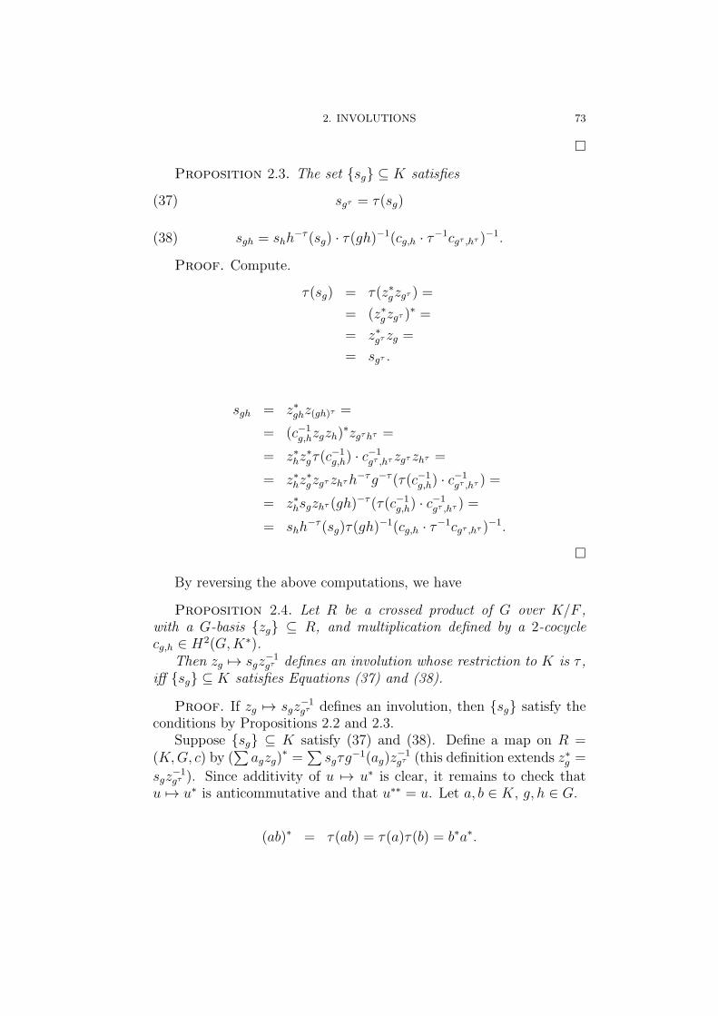
2. INVOLUTIONS 73
Proposition 2.3. The set sg ⊆ K satisfies
(37) sgτ = τ(sg)
(38) sgh = shh−τ (sg) · τ(gh)−1(cg,h · τ−1cgτ ,hτ )−1.
Proof. Compute.
τ(sg) = τ(z∗gzgτ ) =
= (z∗gzgτ )∗ =
= z∗gτ zg =
= sgτ .
sgh = z∗ghz(gh)τ =
= (c−1g,hzgzh)∗zgτhτ =
= z∗hz∗gτ(c
−1g,h) · c
−1gτ ,hτ zgτ zhτ =
= z∗hz∗gzgτ zhτh−τg−τ (τ(c−1g,h) · c
−1gτ ,hτ ) =
= z∗hsgzhτ (gh)−τ (τ(c−1g,h) · c−1gτ ,hτ ) =
= shh−τ (sg)τ(gh)
−1(cg,h · τ−1cgτ ,hτ )−1.
By reversing the above computations, we have
Proposition 2.4. Let R be a crossed product of G over K/F ,with a G-basis zg ⊆ R, and multiplication defined by a 2-cocyclecg,h ∈ H2(G,K∗).
Then zg 7→ sgz−1gτ defines an involution whose restriction to K is τ ,
iff sg ⊆ K satisfies Equations (37) and (38).
Proof. If zg 7→ sgz−1gτ defines an involution, then sg satisfy the
conditions by Propositions 2.2 and 2.3.Suppose sg ⊆ K satisfy (37) and (38). Define a map on R =
(K,G, c) by (∑agzg)
∗ =∑sgτg
−1(ag)z−1gτ (this definition extends z∗g =
sgz−1gτ ). Since additivity of u 7→ u∗ is clear, it remains to check that
u 7→ u∗ is anticommutative and that u∗∗ = u. Let a, b ∈ K, g, h ∈ G.
(ab)∗ = τ(ab) = τ(a)τ(b) = b∗a∗.
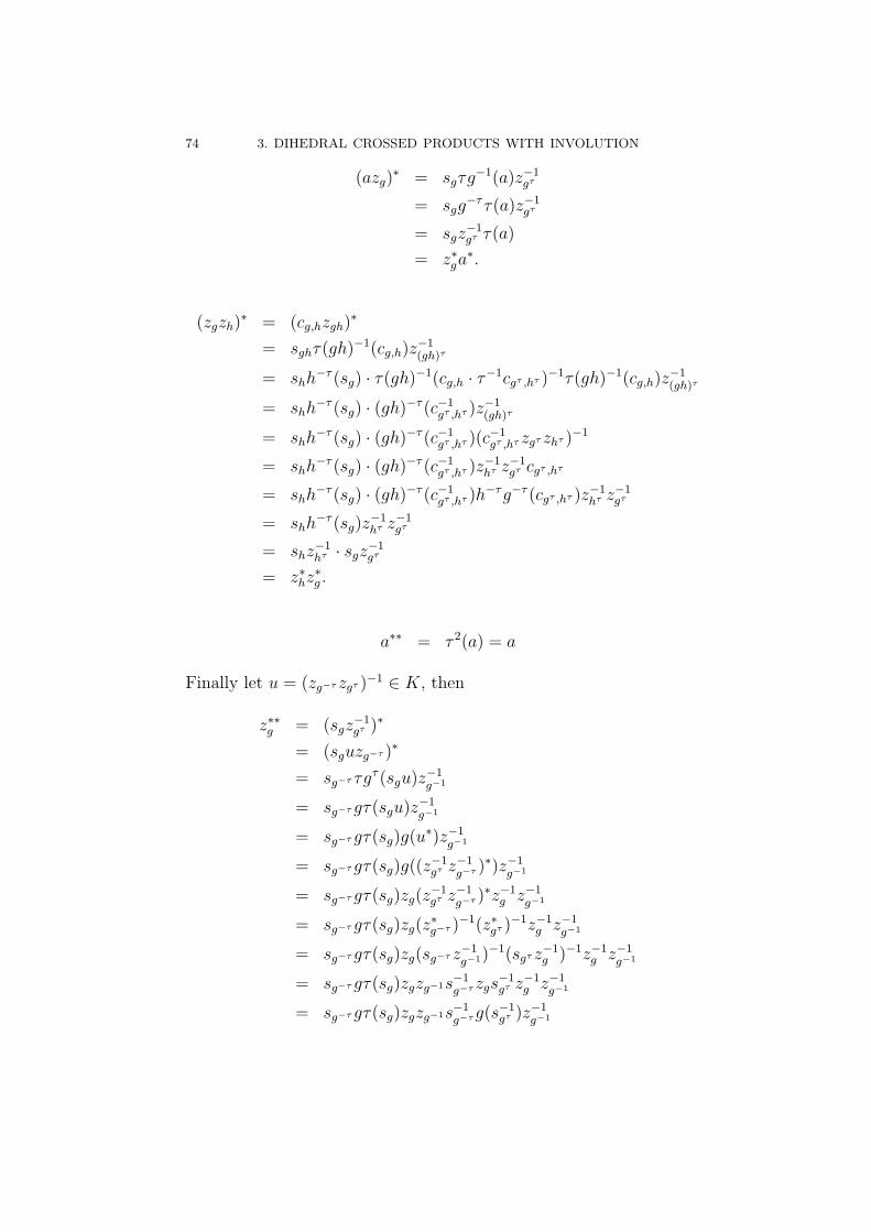
74 3. DIHEDRAL CROSSED PRODUCTS WITH INVOLUTION
(azg)∗ = sgτg
−1(a)z−1gτ
= sgg−ττ(a)z−1gτ
= sgz−1gτ τ(a)
= z∗ga∗.
(zgzh)∗ = (cg,hzgh)
∗
= sghτ(gh)−1(cg,h)z
−1(gh)τ
= shh−τ (sg) · τ(gh)−1(cg,h · τ−1cgτ ,hτ )−1τ(gh)−1(cg,h)z
−1(gh)τ
= shh−τ (sg) · (gh)−τ (c−1gτ ,hτ )z
−1(gh)τ
= shh−τ (sg) · (gh)−τ (c−1gτ ,hτ )(c
−1gτ ,hτ zgτ zhτ )−1
= shh−τ (sg) · (gh)−τ (c−1gτ ,hτ )z
−1hτ z
−1gτ cgτ ,hτ
= shh−τ (sg) · (gh)−τ (c−1gτ ,hτ )h
−τg−τ (cgτ ,hτ )z−1hτ z−1gτ
= shh−τ (sg)z
−1hτ z
−1gτ
= shz−1hτ · sgz−1gτ
= z∗hz∗g .
a∗∗ = τ 2(a) = a
Finally let u = (zg−τ zgτ )−1 ∈ K, then
z∗∗g = (sgz−1gτ )∗
= (sguzg−τ )∗
= sg−τ τgτ (sgu)z−1g−1
= sg−τgτ(sgu)z−1g−1
= sg−τgτ(sg)g(u∗)z−1g−1
= sg−τgτ(sg)g((z−1gτ z
−1g−τ )
∗)z−1g−1
= sg−τgτ(sg)zg(z−1gτ z
−1g−τ )
∗z−1g z−1g−1
= sg−τgτ(sg)zg(z∗g−τ )−1(z∗gτ )
−1z−1g z−1g−1
= sg−τgτ(sg)zg(sg−τ z−1g−1)−1(sgτ z
−1g )−1z−1g z−1g−1
= sg−τgτ(sg)zgzg−1s−1g−τ zgs−1gτ z
−1g z−1g−1
= sg−τgτ(sg)zgzg−1s−1g−τg(s−1gτ )z
−1g−1

2. INVOLUTIONS 75
= sg−τgτ(sg)zgg−1(s−1g−τ g(s
−1gτ ))
= sg−τgτ(sg)s−1g−τg(s
−1gτ )zg
= gτ(sg)g(s−1gτ )zg
= g(τ(sg)s−1gτ )zg
= zg.
Example 2.5. For cyclic algebras G = ⟨g|gn = 1⟩, and we can
choose zgi = zi for z = zg. Then the cocycle becomes cgi,gj = 1 ifi+ j < n, cgi,gj = b1 otherwise, where b = zn ∈ F
For τ = 1, the conditions above translates to NK/F (η) = b2 where
η = sg ∈ K. If n is even and τ = gn/2, then η = sg ∈ Kτ and againNK/F (η) = b2.
Proposition 2.4 is a generalization of the computations done byAlbert [1, Theorems X.16–17] for the case τ = 1, in his proof that Rhas an involution iff exp(R) | 2.
Now let rg = z∗gz−1g−τ = sg(zg−τ zgτ )
−1 ∈ K.
Proposition 2.6.
(39) rg−τ = gτ(r−1g )
Proof. Compute:
gτ(rg) = zg(rg)∗z−1g
= zg(z∗gz−1g−τ )
∗z−1g
= zg(z∗g−τ )−1zgz
−1g
= (z∗g−τ z−1g )−1
= (rg−ta)−1
Corollary 2.7. z∗τ = ±zτ .Proof. We have that τ−τ = τ , so by Equation (39), rτ
2 = 1, thatis z∗τ = ±zτ .
Note that any element zg of a G-basis can be replaced by anotherelement kzg, k ∈ K. If G has exponent 2, then every element of Gsatisfies g−τ = g. In [3, Theorem 2.1] it is shown that in this case zgcan be chosen such that z∗g = ±zg. This can be slightly improved.
Proposition 2.8. If g ∈ G, g = τ , satisfies g−τ = g, then we canchoose zg to satisfy z∗g = zg.
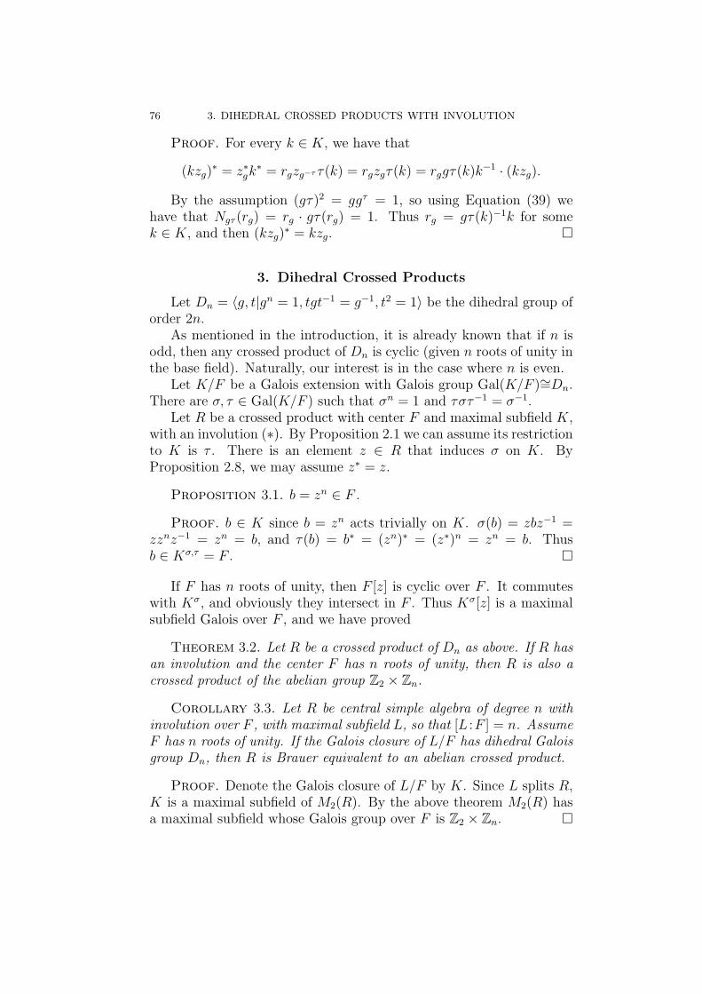
76 3. DIHEDRAL CROSSED PRODUCTS WITH INVOLUTION
Proof. For every k ∈ K, we have that
(kzg)∗ = z∗gk
∗ = rgzg−τ τ(k) = rgzgτ(k) = rggτ(k)k−1 · (kzg).
By the assumption (gτ)2 = ggτ = 1, so using Equation (39) wehave that Ngτ (rg) = rg · gτ(rg) = 1. Thus rg = gτ(k)−1k for somek ∈ K, and then (kzg)
∗ = kzg.
3. Dihedral Crossed Products
Let Dn = ⟨g, t|gn = 1, tgt−1 = g−1, t2 = 1⟩ be the dihedral group oforder 2n.
As mentioned in the introduction, it is already known that if n isodd, then any crossed product of Dn is cyclic (given n roots of unity inthe base field). Naturally, our interest is in the case where n is even.
Let K/F be a Galois extension with Galois group Gal(K/F )∼=Dn.There are σ, τ ∈ Gal(K/F ) such that σn = 1 and τστ−1 = σ−1.
Let R be a crossed product with center F and maximal subfield K,with an involution (∗). By Proposition 2.1 we can assume its restrictionto K is τ . There is an element z ∈ R that induces σ on K. ByProposition 2.8, we may assume z∗ = z.
Proposition 3.1. b = zn ∈ F .
Proof. b ∈ K since b = zn acts trivially on K. σ(b) = zbz−1 =zznz−1 = zn = b, and τ(b) = b∗ = (zn)∗ = (z∗)n = zn = b. Thusb ∈ Kσ,τ = F .
If F has n roots of unity, then F [z] is cyclic over F . It commuteswith Kσ, and obviously they intersect in F . Thus Kσ[z] is a maximalsubfield Galois over F , and we have proved
Theorem 3.2. Let R be a crossed product of Dn as above. If R hasan involution and the center F has n roots of unity, then R is also acrossed product of the abelian group Z2 × Zn.
Corollary 3.3. Let R be central simple algebra of degree n withinvolution over F , with maximal subfield L, so that [L :F ] = n. AssumeF has n roots of unity. If the Galois closure of L/F has dihedral Galoisgroup Dn, then R is Brauer equivalent to an abelian crossed product.
Proof. Denote the Galois closure of L/F by K. Since L splits R,K is a maximal subfield of M2(R). By the above theorem M2(R) hasa maximal subfield whose Galois group over F is Z2 × Zn.
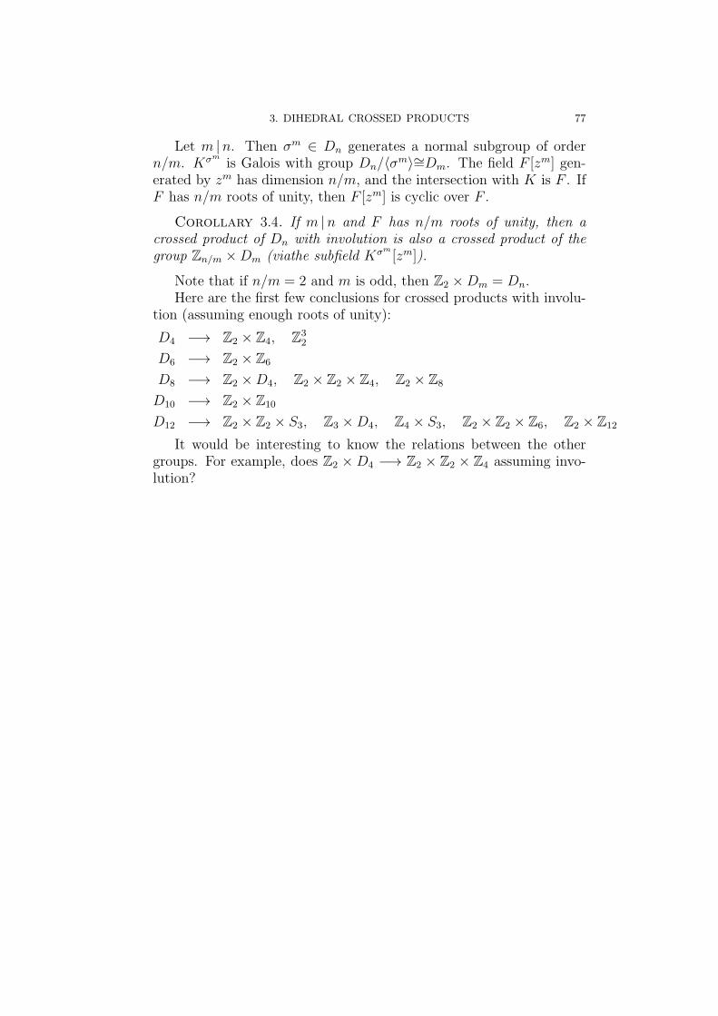
3. DIHEDRAL CROSSED PRODUCTS 77
Let m |n. Then σm ∈ Dn generates a normal subgroup of ordern/m. Kσm
is Galois with group Dn/⟨σm⟩∼=Dm. The field F [zm] gen-erated by zm has dimension n/m, and the intersection with K is F . IfF has n/m roots of unity, then F [zm] is cyclic over F .
Corollary 3.4. If m |n and F has n/m roots of unity, then acrossed product of Dn with involution is also a crossed product of thegroup Zn/m ×Dm (viathe subfield Kσm
[zm]).
Note that if n/m = 2 and m is odd, then Z2 ×Dm = Dn.Here are the first few conclusions for crossed products with involu-
tion (assuming enough roots of unity):
D4 −→ Z2 × Z4, Z32
D6 −→ Z2 × Z6
D8 −→ Z2 ×D4, Z2 × Z2 × Z4, Z2 × Z8
D10 −→ Z2 × Z10
D12 −→ Z2 × Z2 × S3, Z3 ×D4, Z4 × S3, Z2 × Z2 × Z6, Z2 × Z12
It would be interesting to know the relations between the othergroups. For example, does Z2 ×D4 −→ Z2 × Z2 × Z4 assuming invo-lution?

Bibliography
[1] A. A. Albert, Structure of Algebras, Amer. Math. Soc. Coll. Publ., Vol. XXIV,Providence, 1961.
[2] S. Amitsur, On Central Division Algebras, Israel J. Math., 24, 408–420, (1972).[3] S. Amitsur, L. H. Rowen and J.-P. Tignol, Division Algebras of Degree 4 and
8 with Involution, Israel J. Math., 33(2), 133–148, (1979).[4] S. Amitsur and D. Saltman, Generic Abelian Crossed Products and p-Algebras,
J. Algebra, 51(1), 76–87, (1978).[5] S. Amitsur and J.-P. Tignol, Kummer subfields of Malcev-Neumann division
algebras, Israel J. Math., 50, 114–144, (1985).[6] M. Artin, Brauer Severi Varieties, in Brauer groups in ring theory and alge-
braic geometry (Wilrijk, 1981), LNM 917, 194–210, 1982.[7] H. Bass and J. Tate, The Milnor Ring of a Global Field, in Algebraic K-
theory, II: ”Classical” algebraic K-theory and connections with arithmetic(Proc. Conf., Seattle, Wash., Battelle Memorial Inst., 1972), LNM 342, 349–446, 1973.
[8] E. Brussel, Noncrossed Products and Nonabelian crossed products over Q(t)and Q((t)), Amer. J. Math., 117(2), 377–393, (1995).
[9] S. U. Chase, Two Results on Central Simple Algebras, Comm. Algebra, 12,2279–2289, (1984).
[10] P. K. Draxl, Skew Fields, London Math. Soc. Lec. Notes Ser. 81, 1983.[11] S. Eilenberg and S. MacLane, Cohomology and Galois Theory, I. Normality of
Algebras of Teichmuller’s Cocycle, Trans. Amer. Math. Soc., 64, 1–20, (1948).[12] M. D. Fried and M. Jarden, Field Arithmetic, Springer-Verlag, 1986.[13] D. Hilbert, Die Theorie der Algebraichen Zahlk orper, Jahresb. Deut. Math.
Ver., 4, 175–546, (1897).[14] N. Jacobson, Basic Algebra II, W. H. Freeman and Co., San Francisco, Calif.,
1980.[15] N. Jacobson, Finite Dimensional Division Algebras over Fields, Springer, 1996.[16] N. Jacobson, p-algebras of exponent p, Bull. AMS, 43, 667–670, (1937).[17] K. Kato, Galois Cohomology of Complete Discrete Valuation Fields, in Alge-
braic K-theory, Part II (Oberwolfach, 1980), LNM 967, 215–238, 1982.[18] M. A. Knus, M. Ojanguren and D. J. Saltman, On Brauer Groups in Charac-
teristic p, in Brauer groups (Proc. Conf., Northwestern Univ., Evanston, Ill.,1975), LNM 549, 25–49, 1976.
[19] P. Mammone, Sur la corestriction des p-symboles, Comm. Alg., 14(3), 517–529,(1986).
[20] P. Mammone and A. Merkurjev, On the corestriction of pn-symbol, Israel J.Math., 76(1–2), 73–79, (1991).
79

80 BIBLIOGRAPHY
[21] P. Mammone and J.-P. Tignol, Dihedral Algebras are Cyclic, Proc. Amer.Math. Soc., 101(2), 217–218, (1987).
[22] J. C. McConnel, Division Algebras Beyond the Quaternions, Amer. Math.Mont., 105(1), 154–162, (1998).
[23] A. S. Merkurjev, Brauer Groups of Fields, Comm. Alg., 11(22), 2611–2624,(1983).
[24] A. S. Merkurjev, A. A. Suslin, K-cohomology of Severi-Brauer varieties andthe norm residue homomorphism, Izv. Akad. Nauk. SSSR ser. Mat., 46(5),1011–1046, 1135–1136. Trans. Math USSR Izv., 21(2), 307–340, (1983).
[25] L. Ribes, Introduction to profinite groups and Galois cohomology, Queen’sPapers in Pure and Applied Mathematics, 24. Queen’s University, Kingston,ON, 1999.
[26] J. Rosenberg, Algebraic K-Theory and its Applications, Springer-Verlag, 1994.[27] L. H. Rowen, Cyclic Division Algebras, Israel J. Math., 41, 213–234, corr. ibid.
43, 277–280, (1982).[28] L. H. Rowen, Are p-Algebras Having Cyclic Quadratic Extensions Necessarily
Cyclic?, J. Algebra, 215, 205–228, (1999).[29] L. H. Rowen, Central Simple Algebras, Israel J. Math., 29(2–3), 285–301,
(1978).[30] L. H. Rowen, Ring Theory, Academic Press, 1988.[31] L. H. Rowen and D. J. Saltman, Dihedral Algebras are Cyclic, Proc. Amer.
Math. Soc., 84(2), 162–164, (1982).[32] L. H. Rowen and D. J. Saltman, Division Algebras over C2- and C3-fields,
preprint, (2000).[33] L. H. Rowen, J.-P. Tignol, On the Decomposition of Cyclic Algebras, Israel J.
Math., 96, 553–578, (1996).[34] D. J. Saltman, Noncrossed Products of Small Exponent, Proc. Amer. Math.
Soc., 68, 165–168, (1978).[35] D. J. Saltman, Noncrossed product p-algebras and Galois p-extensions, J. Al-
gebra, 52, 302–314, (1978).[36] D. J. Saltman, Azumaya Algebras over Rings of Characteristic p,Doctoral Dis-
sertation, Yale University, 1976.[37] R. L. Snider, Is the Brauer Group Generated by Cyclic Algebras?, in Ring
theory (Proc. Conf., Univ. Waterloo, Waterloo, 1978), LNM 734, 279–301,1979.
[38] A. A. Suslin, Torsion in K2 of fields, K-Theory, 1(1), 5–29, (1987).[39] O. Teichmuller, p-Algebren, Deutsche Math., 1, 362–388, (1936).[40] W. van der Kallen, The Merkurjev-Suslin Theorem, in Orders and their Ap-
plications (Oberwolfach, 1984), LNM 1142, 157–168, 1985.