Central Place Theory and Zipf’s Law

Wen-Tai Hsu∗

July 17, 2008

Abstract

This paper provides a theory of the location of firms and, as cities are groups of firms,the emergence of cities. Using a model of equilibrium entry, this paper provides amicrofoundation for central place theory and the conditions under which Zipf’s lawfor cities emerges. Central place theory describes how a hierarchical city system withdifferent layers of cities serving different sized market areas forms from a uniformlypopulated space. Zipf’s law for cities, that is, the size distribution of cities followingthe Pareto distribution with a tail index close to 1, is a robust empirical regularity. Inthe model, the main force driving the size difference of cities is the tradeoff betweentransportation cost and scale economies, which differs across goods due to differentfixed costs of production. Since a central place hierarchy also implies a hierarchy offirms, Zipf’s law for firms is also approximated. The theory is also consistent witha newly discovered empirical regularity, the number-average-size rule, which is a log-linear relationship between the number of cities and the average size of cities where anindustry is located.

JEL: R12; L11; R13

Keywords: central place theory, Zipf ’s law, number-average-size rule

∗Department of Economics, University of Minnesota, Twin Cities. 1035 Heller Hall, 271 19th Ave S.,Minneapolis, MN 55455. Email: wentai@umn.edu. I am grateful to Tom Holmes, Sam Kortum, and ErzoG. J. Luttmer for their advice and encouragement. I benefit from the discussions and comments fromseminar participants at the University of Minnesota, Federal Reserve Bank of Minneapolis, the University ofChicago, the University of Toronto, and the Doctoral Poster Session of the American Real Estate and UrbanEconomics Association. In particular, I would like to thank Marcus Berliant, V.V. Chari, Gilles Duranton,Willie Fuchs, Xavier Gabaix, Patrick Kehoe, Wen-Chi Liao, Roger Myerson, Derek Neal, Shi Qi, ChristianRedfearn, Maryam Saeedi, Robert Shimer, Aloysius Siow, Nancy Stokey, Evsen Turkay, Matt Turner, HaraldUhlig, Ping Wang, Tianxi Wang, and William Wheaton. All errors are mine. Updated version of this paperis available at http://www.econ.umn.edu/∼tedhsu75/papers.htm.

1

1 Introduction

The distribution of city sizes is highly skewed: there are many more small cities than there

are large cities. Remarkably, the distribution obeys the rank-size rule by which the product

of the rank and the size of a city is a constant. This empirical relationship is also named

Zipf’s law and is shown to be robust across historical and cross-country studies.1

The existence of such a striking empirical relationship calls for explanations, and there

has been much recent theoretical work aimed at providing them. Deriving Zipf’s law from

a steady-state distribution of a random growth process has been the dominant approach,

e.g., Gabaix (1999) and Rossi-Hansberg and Wright (2007).2 In a random growth process,

large cities arise due to long histories of favorable productivity shocks; however, since the

probability of such events are low, there are not many large cities, i.e., a skewed distribution.

Gabaix (1999) explains why the steady state distribution should be Zipf’s. One criticism

concerning this literature is that there is little sense that cities of different sizes play different

roles in the economy.3 Moreover, there are no spatial elements or spatial interactions across

cities. What drives the size differences of cities is simply randomness.

This paper explains Zipf’s law in a spatial model in which cities of different sizes serve

different functions in the economy. It builds on the insights of central place theory, first

developed by the German geographers Christaller (1933) and Losch (1940). The idea of the

theory is that goods differ in the degree of scale economies relative to market size. Goods

with substantial scale economies, e.g., stock exchanges or symphony orchestras, will only

be found in a few places, while other goods with low scale economies, e.g., gas stations

or convenience stores, will be found in many places. Moreover, large cities tend to have

a wide range of goods, while small cities only provide goods with low scale economies.

Naturally, small cities are in the market areas of large cities for those goods that they do

not provide. In Christaller’s scheme, the hierarchy property4 holds if larger cities provide all

goods that smaller cities provide. We can readily see that this setup implies a skewed city

size distribution.

In this paper, a city system has multiple layers of cities, and the cities of the same layer

1Zipf’s law has its name following Zipf (1949). However, the discovery of Zipf’s law may be as early asAuerbach (1913). For more details regarding Zipf’s law, see Section 2 or Gabaix and Ioannides (2004).

2Early explanations date back to Zipf (1949), Champernowne (1953), and Simon (1955). Gabaix (1999),Cordoba (2003), and Rossi-Hansberg and Wright (2007) based their theories on providing a microfoundationfor Gibrat’s law. Also see Berliant and Watanabe (2007), Brakman, Garretsen, and van den Berg (1999,2001), Chen (2004), Duranton (2006, 2007), Eeckhout (2004), Reed (2001; 2002), Reed and Huges (2002).See Kali (2003) for a random graph approach.

3Combining the random growth approach and the type-of-cities theory of Henderson (1974), Rossi-Hansberg and Wright (2007) are an exception. Nonetheless, their model has the feature that any cityspecializes in only one industry. More discussion about this will follow.

4This is often referred to as the hierarchy principle in the literature.

2

have the same functions, i.e., host the same set of industries. For simplicity, the geographic

space is assumed to be the real line. The model can be viewed as a multiple-good extension

to Lederer and Hurter (1986), in which firms play a two-stage game: firms compete in

price at each local market after making their location choices. The driving force behind

the differentiation of cities is the heterogeneity of scale economies among goods, which is

modeled by heterogeneity in the fixed cost of production.5 Two important results are that a

class of equilibria consistent with the hierarchy property exists, and that there is always only

one next-layer city in between two neighboring larger cities. The second result, for which

I call the central place property, implies that the ratio of the market areas of one layer to

the next is 2, and it is analogous to the K = 3 market principle of Christaller (1933).6 In

this paper, a central place hierarchy is a city system in which both the hierarchy and central

place properties hold .

This paper does four things.

First, it microfounds central place theory. Although central place theory has a long

history in economic geography, its modeling has been mechanical. (See Chapter 3.1 of

Fujita et al. (2001) and Berliant (2005) for critiques of the lack of microfoundations in

this literature.) A few attempts to formalize central place theory have been made in the

economics literature. Fujita, Krugman, and Mori (1999) generated a hierarchical city system

through an evolutionary approach to extend a core-periphery model of Fujita and Mori

(1997). Given the existence of the first and largest city, Fujita et al. (1999) successfully

modeled the hierarchy property.7 Compared to this paper, however, their model is relatively

complicated, the location pattern of cities does not feature the central place property, and

their model do not lead to Zipf’s law.

Second, this paper specifies the conditions under which the city size distribution is not

only skewed, but in fact, obeys Zipf’s law. Note that this is not the first paper explaining

Zipf’s law via central place theory, since Beckmann (1958) already did so through a mathe-

matical treatment of a hierarchical structure.8 Nonetheless, similar to most previous central

place theory studies, he did not provide a microfoundation for his treatment. I prove that

Zipf’s law emerges when the number of layers in a city hierarchy is large enough. The fun-

damental reasoning behind Zipf’s law is that the rank of cities doubles from one layer to the

next (i.e., the central place property), while the sizes of cities shrink at a rate close to one

5Alternatively, one can model the heterogeneity of scale economies by the heterogeneity in demands acrossgoods. The model in this paper can be easily transformed in this way.

6In the extension to the plane, which can be easily done, if there is always only one next-layer city locatedin the equilateral triangle area in between three neighboring larger cities, this ratio of market areas is 3.

7Another attempt is by Eaton and Lipsey (1982), who modeled the co-location of two retail stores (eachselling a distinct good) and their coexistence with one-store locations in a spatial competition model.

8Fujita et al. (2001) were obviously aware of the link between central place theory and Zipf’s law, butthey could not establish this link. See Chapter 11 and 12.

3

half, since when this rate is exactly one half, the rank-size rule holds. A numerical exercise

conducted in this paper verifies the result and shows how fast the convergence to Zipf’s law

is achieved.

Third, the model is also consistent with a newly discovered empirical regularity called the

number-average-size (NAS) rule, which was first documented from Japanese urban-industrial

data by Mori, Nishikimi, and Smith (2007). The NAS rule states that the relationship

between the number of cities and the average size of cities where an industry is located is

linear on a log-log scale with a negative slope. To illustrate the definition, suppose Major

League Baseball is an industry. Since there are 26 cities (MSA’s) that host at least one

baseball team, the number of concern is 26, and the average size of concern is the average

population of these 26 cities.9 In this paper, I document that the NAS rule also holds for the

US. Notice that central place theory already implies that the number and average sizes are

negatively related. Moreover, Mori et al. (2007) show that this new empirical regularity is

essentially equivalent to Zipf’s law, provided that the hierarchy property holds.10 Therefore,

since the model in this paper has both the hierarchy property and Zipf’s law, the NAS

rule holds. It is worth emphasizing that the link between Zipf’s law and the NAS rule

demonstrates the importance of the insights of central place theory regarding the formation

of an urban system. In contrast, urban theories based on the random growth approach and/or

the type-of-cities approach have little explanatory power in this respect. In the type-of-cities

theory of urban systems, e.g., Henderson (1974) and Rossi-Hansberg and Wright (2007),

each city specializes in only one industry, and city size differs due to industrial differences in

production technology.

Fourth, this paper also derives Zipf’s law for firms.11 Notice that a central place hierarchy,

indeed, also leads to a hierarchy of firms since those firms located exclusively in large cities

serve larger market areas (i.e., more consumers) and must be larger. Using US data, Holmes

and Stevens (2004) established a robust fact that within an industry, areas of industrial

concentration tend to have larger plants. This provides a different angle from the literature

of explaining Zipf’s law for firms, which also predominantly draws upon random growth

processes. See, for examples, Luttmer (2007) and Simon and Bonini (1958).

There are two steps in the modeling in this paper. In the first step, a basic model is

developed to deliver the fundamental hierarchical structure. Simple closed form solution is

9On the other hand, it is obvious that for the industry of gas stations, the number is larger than 26, andthe average size is smaller.

10In Mori et al. (2007), the hierarchy property (they called it the hierarchy principle) states that if anindustry is present in a city of a certain size, it is present in all cities of larger sizes. Note that this isequivalent to the hierarchy property of Christaller (1933) – cities of higher order provide all goods that citiesof lower order provide, assuming that the relationship between “industries” and “goods” is one-to-one.

11For evidence on Zipf’s law for firms, see Axtell (2001) and Luttmer (2007). Also, see the discussion inSection 2.

4

readily obtained in the basic model, and this provides a tractable framework for studying

the conditions for Zipf’s laws and the NAS rule. Nonetheless, the equilibria giving rise to

central place hierarchies are only a subset of all possible equilibria, and there is no particular

argument favoring this special type of equilibria. Moreover, the hierarchies in the basic

model emerges from the interactions of two types of agents: firms and farmers. There is no

role for city workers, and, hence, the size definitions of cities is not by populations in cities.

The general model provides remedies for both problems, by incorporating workers and using

the home market effect (because firms sell to local workers) to provide an agglomeration

force favoring the type of equilibria with hierarchical structure. The drawback of the general

model is that it no longer has a closed form solution, and one needs numerical exercises to

check the robustness of the Zipf’s law results.

The model, as is, has an empirical implication regarding the distribution of economic

activities within a metropolitan area. More discussions on this implication will follow in the

conclusion.

This paper models central place hierarchies as equilibrium results. A companion paper

(Hsu, 2008) presents a detailed examination of the efficiency properties of central place

hierarchies. In particular, central place hierarchy equilibria are, in general, suboptimal.

However, conditional on the hierarchy property, the optimal central place hierarchy exhibits

similar location pattern to that in equilibrium and, hence, delivers Zipf’s law and the NAS

rule.

The rest of this paper is organized as follows. Section 2 describes the empirical regularities

that concern this paper in greater detail, especially the NAS rule for the US, since it is first

documented here. Section 3 lays out the basic model and derives central place hierarchies as

equilibrium results. Section 4 specifies the conditions under which Zipf’s laws and the NAS

rule hold. Section 5 generalizes the model to add workers’s location decisions and shows the

robustness of the Zipf’s law results. Section 6 concludes.

2 Empirical Regularities

The purpose of this section is two-fold: to provide more details of the empirical evidence on

Zipf’s laws and central place theory, and to document the NAS rule for the US.

2.1 Zipf’s laws and central place theory

Zipf’s law for cities has been well-documented. Detailed empirical issues, as well as a survey

of the theoretical literature, may be found in Gabaix and Ioannides (2004). The following

quickly gives readers an idea.

5

0.1 1 10 1001

10

100

1000

Size (millions; log scale)

Ran

k (lo

g sc

ale)

Zipf’s Plot for All MSA’s (2000 US Census)

OLS: y= − 0.9491*x+16.88, R2=0.9857Adjusted OLS: y= − 0.9699*x+17.14

Figure 1: Zipf’s plot for all 362 Metropolitan Statistical Areas.

The observation of Zipf’s law for cities is most clear when one plots city ranks against

city sizes on a log-log scale, that is, Zipf’s plot. Figure 1 presents a Zipf’s plot using US

2000 census data for all MSA’s, i.e., Metropolitan Statistical Areas. The OLS regression of

the log of rank on the log of size of all 362 MSA’s (metropolitan statistical areas) entails an

R2 of 0.9857 and a slope of −0.9491. While the fact that a straight line fits fairly well leads

one to believe that the size distribution of cities follows the Pareto distribution,12 defined by

the tail probability

P (S > s) =a

sζ, s ≥ s,

for some positive constants a and s and the tail index13 ζ, historical and cross-country studies

show that the tail index ζ is approximately 1.14 When ζ = 1, the product of the rank and

size of a city is a constant, the rank-size rule, which is an attractive interpretation of Zipf’s

law. It means that the size of the second largest city (e.g., L.A.) is (approximately) half of

the largest (e.g., New York) and that of the third largest (e.g., Chicago) is one-third of the

largest, etc.

One should note that, positing the Pareto distribution, the OLS estimation is biased

and typically underestimates the true tail index.15 Gabaix and Ibragimov (2007) propose an

adjusted OLS method that minimizes this bias. By their method, one runs a regression of

12Eeckhout (2004) argues that the size distribution of cities should follow a lognormal distribution whenall cities (i.e., human settlements) are considered. Also, see Holmes and Lee (2007) for their discussion onthe work of Eeckhout (2004).

13The empirical literature on size distributions sometimes call this Zipf’s coefficient. In this paper, thetail index, Zipf’s coefficient, and the slope of a Zipf’s plot are used interchangeably.

14See Gabaix and Ioannides (2004) for a detailed examination.15See Gabaix and Ioannides (2004) and Gabaix and Ibragimov (2007). On the other hand, the OLS

estimator is still consistent.

6

the log of rank−12

on the log of size. The estimated tail index for the 362 MSA’s of the US

2000 census data is 0.9699. To test ζ = 1, the (asymptotic) standard error is 0.0743. With

a 5% level of significance, one does not reject the hypothesis of ζ = 1.

It is also a robust fact that there are deviations from Zipf’s law in both very large and very

small cities.16 Rossi-Hansberg and Wright (2007) provide a model capturing this property.

This fact can also be matched in this paper.17

The regular shape of firm size distribution has been noted several decades ago, e.g.,

Simon and Bonini (1958), Steindl (1965), and the general perception was that the firm

size distribution overall fit a log-normal distribution, while its upper tail fit the Pareto

distribution or Zipf’s law. Nonetheless, using the 1997 US economic census, Axtell (2001)

documents the size distribution for all tax-paying firms in the US, showing that Zipf’s law

fits fairly well for the overall distribution. Luttmer (2007) does the same for 2002 and has

similar results. The estimates of tail indices from the two papers mentioned were both 1.06;

close to, but above 1.

The empirical literature in economic geography regarding central place theory consists

mostly of case studies. The earliest efforts surround the spatial patterns of human settle-

ments, and the most notable example is, of course, Christaller (1933)’s study of the spatial

patterns of cities and towns in Southern Germany, which seems to fit the assumption of

the homogeneous farming plain. Furthermore, Berry and Garrison (1958a,b) provide case

studies regarding the sizes and functions of central places in Snohomish County, Washington.

Few empirical studies have tried to examine the main propositions/assumptions of central

place theory using large-scale data, such as national data, until Mori et al. (2007). They

documented two empirical regularities: the hierarchy property and the NAS rule, using

Japanese urban-industrial data. Using 3-digit classifications of industries, they found that

71% of industries present in certain cities are also present in all larger sized cities. Moreover,

they show that this finding is unlikely to be a random event. I have also examined the

evidence of the hierarchy property by using US data. It seems that the hierarchy property

also holds for the US. However, this detail is omitted from this paper.

2.2 The NAS rule

Recall that the number-average-size (NAS) Rule states that the number of cities and the

average size of the cities where an industry is located follow a log-linear relationship. In

16Again, see Gabaix and Ioannides (2004).17In this paper, the slight concavity of Zipf’s plot emerges from the fact that the existence of any city

requires a market area (scale economies) above some critical level. In Rossi-Hansberg and Wright (2007),each city specializes in only one industry; therefore, city size distribution is tied closely to industry-specificshocks. Small (Large) cities grow faster (slower) than the mean growth rate because they have small (large)stocks of capital due to decreasing returns.

7

30 53 95 169 300

0.8

1.1

1.6

2.3

3.3

Number (log scale)

Ave

rage

Siz

e (m

illio

n; lo

g sc

ale)

NAS Plot (3−digit NAICS)

Figure 2: number-average-size Plot for US industries classified by 3-digit NAICS.

Mori et al. (2007), the regressions of the log of the average size on the log of the number for

the three-digit industries of Japan (JSIC) of 1980/1981 and 1999/2000 entail R2s that are

both over 0.99, with slopes being −0.7204/− 0.7124.

Using County Business Pattern Data,18 I document that the NAS rule also holds for the

US. Figure 2 shows the number-average-size (NAS) plot (log of average size on the vertical

axis and the log of number on the horizontal axis) for the 77 3-digit NAICS19 with the cities

defined by MSA’s/CMSA’s.20 The “presence” of an industry in an MSA (or a CMSA) is any

positive employment.

The OLS regression gives

log(averagesize) = 17.789

(0.0141)

− 0.7477

(.00255)

log(number), R2 = 0.9991,

where the numbers in the parentheses are the standard errors.

A straight line almost perfectly fits! 21

18Here, the County Business Pattern Data are taken from the compiled data by Holmes and Stevens(2004). The data are available at http://www.econ.umn.edu/∼holmes/data/CBP/index.htm. I thank TomHolmes for helping me with the data.

19NAICS stands for the North American Industry Classification System, and the NAICS used is the 1997version. Similar to Mori et al. (2007), I excluded the sectors of Agriculture, Forestry, Fishing and Hunting(11), and Mining (21), since they are not considered as central place functions. Public Administration (92)was also excluded, since its locations are not determined solely by economic incentives and could be arbitrary.

20CMSA stands for combined metropolitan statistical areas.21Although the plot shown in Figure 2 consists of 77 3-digit NAICS, 51 of them are located in all MSA’s;

thus, they have the same number (267) and average size (813544). In light of the limited number of infor-mative sample points in 3-digit NAICS, it is important to note the robustness of the NAS rule in 4-digitNAICS (shown in Figure 3). Also, out of 77 industries, 21 of them are in the manufacturing sector.

8

One naturally wonders how the NAS plot and the regression result change if one changes

the digit of the NAICS or the threshold of “presence.” Figure 3 shows 4 variations: 3-digit

NAICS and presence defined by employment of at least 50 people (left-top), 3-digit NAICS

and the threshold of employment of at least 100 people (right-top), 4-digit NAICS and any

positive employment (left-bottom), and 4-digit NAICS and the threshold of at least 50 people

(right-bottom).22 The (R2, slope) pairs are (0.997, −0.737), (0.994, −0.721), (0.988, −0.694),

and (0.944, −0.622), respectively. Overall, the log-linear relationship is robust across the

variations of the definitions of industry and presence.

30 53 95 169 300

0.8

1.1

1.6

2.3

3.3

Number (log scale)

Ave

rage

Siz

e (m

illio

n; lo

g sc

ale)

NAS Plot (3−digit NAICS, threshold: 50)

30 53 95 169 300

0.8

1.1

1.6

2.3

3.3

Number (log scale)

Ave

rage

Siz

e (m

illio

n; lo

g sc

ale)

NAS Plot (3−digit NAICS, threshold: 100)

30 53 95 169 300

0.8

1.1

1.6

2.3

3.3

Number (log scale)

Ave

rage

Siz

e (m

illio

n; lo

g sc

ale)

NAS Plot (4−digit NAICS)

30 53 95 169 300

0.8

1.1

1.6

2.3

3.3

Number (log scale)

Ave

rage

Siz

e (m

illio

n; lo

g sc

ale)

NAS Plot (4−digit NAICS, threshold: 50)

Figure 3: number-average-size plots for different industry definitions and thresholds of em-

ployment.

One observes that all slopes of the four variations are all smaller than the slope of the

benchmark case of 3-digit NAICS and any positive employment. There are two clear reasons

as to why this is the case. First, as the threshold is higher, one expects that given the average

size, the number of cities should decrease. Therefore, the slope of the NAS regression line

22To determine which MSA/CMSA is to be excluded by the threshold, I use business employment data inCBP by industry and by county. For establishments with more than 1, 000 employment, I use cell counts bysize class, industry and county from Holmes and Stevens (2004). As shown in Holmes and Steven (2004),the employment size classes in CBP can be deemed as a fine grid, and the true mean (using national data)in each size class should be a close enough approximation.

9

becomes flatter compared to the benchmark case. Second, it is harder for the finer classified

industries to satisfy the hierarchy property. Suppose that the hierarchy property holds

perfectly for an industry, and that the number of cities that host this industry is given by n.

Then, the average size of cities hosting this industry is the average size of the first n largest

cities; this average size is, in fact, the upper bound of the average size of any arbitrary n

cities. Thus, if the hierarchy property holds perfectly, the actual NAS plot will be the same

as the upper average-size plot. Since the hierarchy property holds to a lesser degree with a

finer classification of industries, the slopes of the NAS plot becomes flatter compared to the

upper average-size plot because of the decrease in average size, given the number of cities.

Interestingly, the discrepancy between the actual NAS plot and the upper average-size plot

provides a clue as to how to test the robustness of the hierarchy property.

3 Central Place Theory: the Basic Model

In this section, I present a basic model in which central place hierarchies arise in equilibria.

3.1 Model Setup

3.1.1 Geography, goods, and agents

The geographic space is the real line, and the location is indexed as x ∈ R. There is a [0, 1]

continuum of consumption goods. There are two types of agents: farmers and firms. There

will be workers as a third type of agents in the general model, and they are completely

mobile. In contrast, farmers are completely immobile and are uniformly distributed on the

real line with a density of 1. Each farmer demands one unit of each good in [0, 1]. Imagining

looking at the spatial economy on a very large scale, we virtually view all goods as necessities.

For any good, production requires fixed cost to set up production at a location. Denote

the fixed cost of production for a good as y, and denote the distribution function of fixed

costs as F : [y, y] ⊂ R+ → [0, 1].23 For each good, to produce one unit requires a constant

marginal cost c. The transportation cost is t per unit per mile traveled.

3.1.2 Two-stage game

For each good, there is an infinite pool of potential firms. Assume that each entrant firm

sets up only at one location. The firms and farmers play the following two-stage game:

1. Entry and location stage:

Firms simultaneously decide whether to enter, and upon entering, they must decide

23The left end of the support can be open.

10

their locations. Firms need to pay the fixed cost to set up at the location. Assume the

tie-breaking rule that if a potential firm sees a zero-profit opportunity, it enters.

2. Price competition stage:

Firms deliver goods to farmers. Given the locations of firms, each firm sets a (delivered)

price schedule over the real line. For each good, each location on the real line is a market

in which firms engage in Bertrand competition. For each good, each farmer decides to

buy from which firm.

The model can be viewed as an extension to the spatial market model with price dis-

crimination of Lederer and Hurter (1986) to a continuum of goods.24 25

Definition 1. An equilibrium is a collection of SPNE for each good.

In the following, we study a particular type of equilibria.

3.2 Hierarchy Equilibrium

A hierarchy equilibrium is one in which the hierarchy property holds. Equivalently, we have

Definition 2. A hierarchy equilibrium in an equilibrium in which at any location of produc-

tion, the set of goods produced must be of the form [y, y] for some y.

Goods differ only in fixed costs. Thus, ignoring fixed costs makes the following derivation

of gross profit (i.e., gross of fixed cost) for one good applicable to all goods. Consider two

neighboring firms with a distance of L. Denote the firm on the left-hand side A and that

on the right-hand side B. The marginal costs of delivering the good to a consumer who is x

distance apart from A are thus

MCA =c + tx,

MCB =c + t(L− x).

24The model is different from that of Lederer and Hurter (1986) in many ways, e.g., they consider thecompetition of (only) two firms with a general production technology and a general distribution of demandover a geographic space. Nonetheless, the market mechanism is the same – a two-stage game with firmsdelivering goods.

25What really distinguishes the spatial market models with price discrimination and the spatial competitionmodels, in which firms charge uniform prices, is who bears the transportation cost. It is not clear as to whichmechanism is more realistic. However, it can be shown that there exists no equilibrium in which the hierarchyproperty holds in the spatial competition version of the model in which the transportation cost is borne bythe consumers. I have developed an alternative model of a central place hierarchy in which the transportationcost is borne by the consumers, and the hierarchy property holds partially. This alternative model builds onthe work of Salop (1979) and Vogel (2007). In particular, using the framework in Vogel (2007), the model isfree from the problem of the nonexistence of price equilibrium.

11

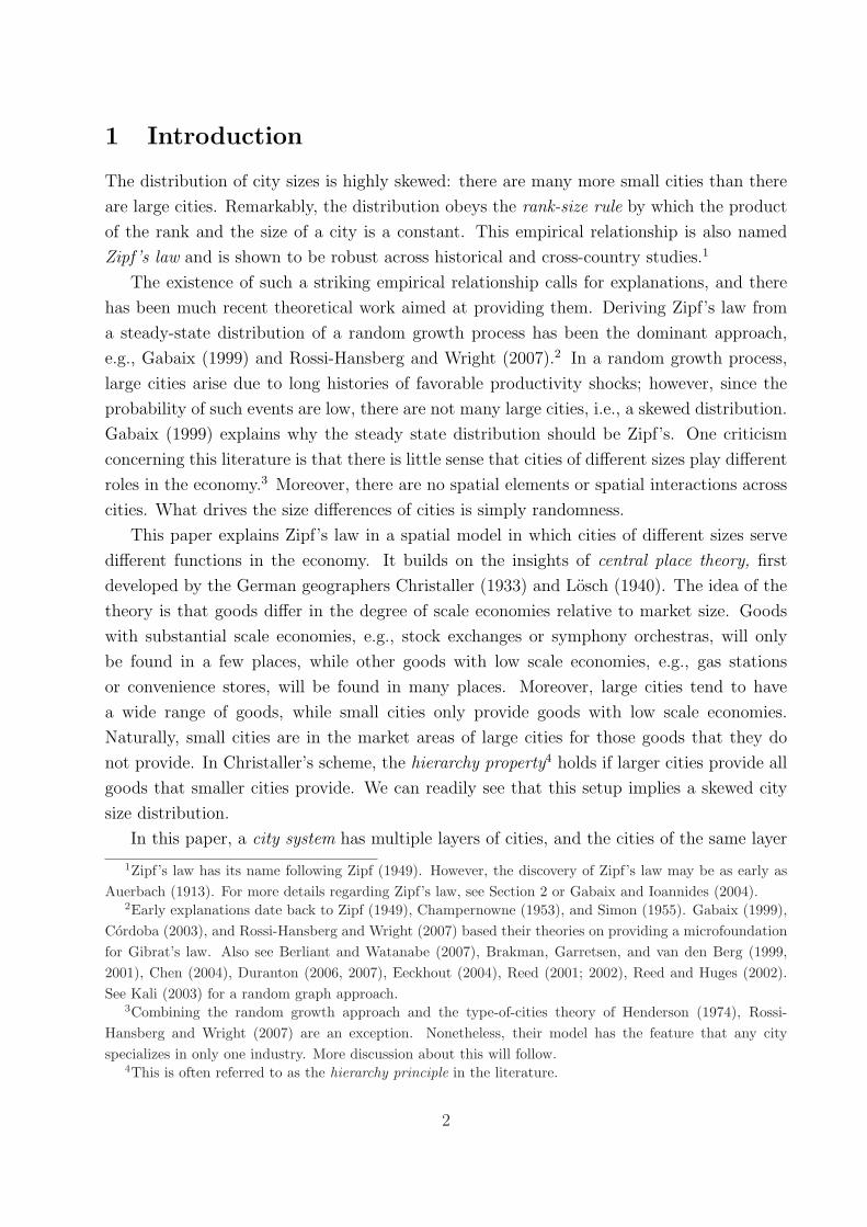
Bertrand competition at each x results in the firm with the lower marginal cost grabbing

the market and charging the price of its opponent’s marginal cost. Thus, the equilibrium

price, given the distance L, is

p(x) =

{c + t(L− x) x ∈ [0, L

2]

c + tx x ∈ [L2, L]

Obviously, the gross profit for firm A from the market area on its right-hand side and

that for B from its left-hand side are both tL2

4. Figure 4 illustrates the marginal cost of both

firms and the equilibrium price, as well as the gross profits from the market area between A

and B.

0

PA PB

MCA = c + txMCB = c + t (L-x)

c

X

$

c+tL

A B

L

2

L

Figure 4: Second-stage competition: Prices and gross profits

Consider any entrant’s strategy at the first stage. Let this entrant be named C. If C

were to enter into a market area between A and B, it is straightforward that C’s profit

maximizing location is right in the middle between A and B, given A and B’s locations. Any

deviation from the middle will strictly decrease C’s profit, and C would enter if and only if

this maximal profit is nonnegative. Therefore, firms must be an equal distance apart, and

the gross profit of any firm with a market area of L is tL2

2.26

The above derivation of a sub-game perfect Nash equilibrium for an arbitrary good leads

to Lemma 1.

26Notice that there is no room for arbitrage; therefore, firms can price discriminate effectively. To see this,refer to Figure 4. For any consumer located at x ∈ [0, L

2 ], the marginal cost of selling the product that shepurchases at x to some consumers to her left is the same as MCB = PA, and the marginal cost of selling theproduct to some consumers to her right must be at least as large as the equilibrium price. Thus, there is noway she could gain any profit by reselling the product.

12

Lemma 1. Fix some y and define L[y] to be the solution to the zero-profit condition tL2[y]2

=

y. Thus, L[y] =√

2yt. There is a continuum of equilibria in which one firm is located at every

point in {x + nL}∞n=−∞, where L ∈ [L[y], 2L[y]) and x ∈ [0, L[y]).

There is a continuum of equilibria because any entrant in between two firms with L2

distance must earn a negative profit, since L2

< L[y].

Notice that the hierarchy property, together with an inelastic demand, implies that the

set of goods that any location of production provides must be in the form of an interval of

[y, y] for some y. Barring a degenerate F , there exists a decreasing sequence y = y1 > y2 >

... > yI ≥ y, for some I, denoting the cutoffs of the ranges of goods produced in different

locations. A hierarchy equilibrium is said to satisfy the central place property if the market

area of firms producing (yi+1, yi] is half of that of firms producing (yi, yi−1].

Definition 3. A hierarchy equilibrium satisfying the central place property is called a central

place hierarchy. A central place hierarchy is characterized by a decreasing sequence of {yi}Ii=2,

such that y ≡ y1 > y2 > ... > yI ≥ yI+1 ≡ y, and firms producing goods in (yi+1, yi] are an

equal distance apart by Li = L1

2i−1 , i ∈ 1, 2, ..., I. Due to the hierarchy property, any location

of production produces goods in the range of [0, yi], and it is called a layer-i city.

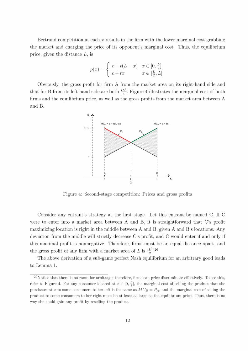
The following proposition constructs a continuum of hierarchy equilibria and shows that

any hierarchy equilibrium satisfies the central place property. Moreover, conditional on the

distance between two layer-1 cities, the hierarchy equilibrium is unique. Therefore, the

multiplicity comes from the distance of L1 = mL[y], m ∈ [1, 2). Call m the multiplicity

factor. An example of a central place hierarchy is illustrated in Figure 5.

Proposition 1 (Central place hierarchy when r ≤ c). Suppose that r ≤ c. For each L1 =

mL[y], m ∈ [1, 2), define Li = L1

2i−1 ,∀i ≥ 2 and construct the cutoffs {yi}Ii=2 to solve the

zero-profit conditionstL2

i

2= yi. Then, for each m ∈ [1, 2), there exists a unique hierarchy

equilibrium in which all type-y firms with y ∈ (yi+1, yi] are Li distance apart. The number of

layers is given by

I = x2 ln m + ln y − ln y

2 ln 2+ 1y, (1)

where xy denotes the floor of a real number. Moreover, any hierarchy equilibrium satisfies

the central place property.

Proof. Referring to Lemma 1, fix an x ∈ R. Make the grid for (yi+1, yi] {x + nLi}∞n=−∞ on

the real line so that any location of firms has goods in the form of [y, yi] for some i. This way,

the location configuration already satisfies the hierarchy property. For any y ∈ (yi+1, yi],

Li

2= Li+1 = L[yi+1] < L[y] ≤ L[yi] ≤ Li,

13

x

x

_

y_

y

y2

y3

y3

0 L1

2

L1

t L 2

2

= y

2

2

t L 3

2

= y

3

2

Figure 5: A typical hierarchy equilibrium.

where the last weak inequality is, indeed, an equality except for i = 1. Therefore, for any

y ∈ (yi+1, yi], firms are Li distance apart with L[y] ≤ Li < 2L[y]. By Lemma 1, each good is

in equilibrium.

Note that the gross profitstL2

i

2shrink over layers toward 0. Therefore, the number of

layers I is infinite if and only if y = 0. Suppose that y > 0; then the formula for I is derived

fromtL2

I

2≥ y and

tL2I+1

2< y. Notice that (1) already implies I = ∞ if y = 0.

To see that any hierarchy equilibrium satisfies the central place property, I show that the

continuum of equilibria so constructed exhausts all hierarchy equilibria. In any hierarchy

equilibrium, all firms are an equal distance apart. Suppose there are ni ∈ N layer-i cities in

between two neighboring larger cities. Clearly, yi firms must earn zero profits and must have

a market area of L′ni

, where L′ is the market area of good in (yi, yi−1]. However, if ni > 1,

it is always profitable for a firm producing a y slightly larger than yi to enter in the middle

between two cities that host (yi, yi−1]. Therefore, ni = 1 for all i.

Apparently, given any hierarchy equilibrium, deviations of firms in a subset of [y, y] by

moving their locations by the same distance and in the same direction change nothing in

terms of pricing and profits. Hence, there is no particular reason why the hierarchy equilibria

are more plausible than others. Even when we begin with a hierarchy equilibrium, there are

no forces preventing the described deviation from happening.

To address this problem, Section 5 provides a model in which workers also enter simulta-

neously with firms in the first stage of the game. Assuming infinite commuting cost, workers

will enter at locations where firms set up. If firms, in addition to their sales to farmers, sell

to local workers, a home market effect is generated. Indeed, this agglomeration force can

14

prevent the above-mentioned deviation.

On the other hand, the general model does not provide closed-form solutions as the basic

model does. Hence, I will investigate the conditions under which Zipf’s laws and the NAS

rule hold under the basic model. I will then show numerically the robustness of Zipf’s laws

and the NAS rule under the general model.

4 Zipf’s Laws and the NAS Rule

In this section, I examine the conditions under which Zipf’s laws and the NAS rule hold

in a central place hierarchy. One common requirement for all cases is that either there are

infinite layers, or the number of layers is large enough.

4.1 Zipf’s Law for Cities

In a central place hierarchy, all firms in the range (yk+1, yk] produce for a market of size Lk.

Thus, the output of firms in this range is Lk(F (yk) − F (yk+1)). Define the size of a layer-i

city by its total units sold to farmers:

Yi =I∑

k=i

Lk(F (yk)− F (yk+1)).

Figure 6 shows an illustration of the definitions of Yi. The green (dark) and red (light) areas

represent the total quantity produced in a layer-1 and layer-2 city, respectively. Notice that

if we assume that the marginal cost takes labor, and if the commuting cost is zero, this

definition of city size is actually proportional to the “working/commuting” population of a

layer-i city.27

Per layer-1 city, there is one layer-2 city and 2i−2 layer-i cities. Thus, the total number

of cities up to layer-i is

Ri = 1 + 1 +i∑

k=3

2k−2 = 2i−1.

We are interested in the relationship between the size Yi and Ri, which approximates the

ranks of layer-i cities. Notice that since the rank doubles from one layer to the next, Zipf’s

law is approximated if the city size Yi approximately shrinks in half from one layer to the

next.

27As an interesting contrast, the general model in Section 5 can be viewed as a case where the commutingcost is infinite so that workers reside at the locations of productions as point masses.

15

0 L1

1 1

Y1

Y2

Y3

Y4

F(y2)

F(y3 )

F(y4 )

L1

2

-L1

2

Figure 6: Total quantities produced in a layer-1 and layer-2 city.

4.1.1 The mechanical condition for Zipf’s law

There is, indeed, a simple but powerful condition linking directly a central place hierarchy

and Zipf’s law for cities, regardless of what the underlying economics behind the hierarchy

is. Given a central place hierarchy, the location patterns of cities of different layers are fixed,

and, hence, different economics would matter only for how the fractions of goods in different

layers are determined.28 The following proposition is a theorem based on fractions of goods

(zi), and this provides a clearer view as to how the propositions based on the fundamentals

of this model (i.e., F (.), since zi = F (yi)) work. This proposition is then useful in cases

where other mechanisms for central place hierarchies are provided by future researches.

Proposition 2 (Bounds on fraction ratios). Suppose that there are infinitely many layers

in a central place hierarchy. Let zi denote the fraction of goods produced in a layer-i city,

and let ∆k = zk − zk+1. Suppose there is a ρ > 1 such that for all i ∈ N,

1

ρ≤ ∆i+1

∆i

≤ ρ.

Then,

1

2(1

ρ− 1) ≤ Yi+1

Yi

− 1

2≤ 1

2(ρ− 1).

Proof. Observe

Yi ∝∞∑

k=i

∆k

2k.

28For example, instead of using heterogeneity of fixed costs among goods, one can use a model of heteroge-nous demand to generate a central place hierarchy.

16

For weights wk,i =∆i+k

2i+k∑∞k=0

∆i+k

2i+k

,

Yi+1

Yi

− 1

2=

1

2

∞∑

k=0

wk,i

(∆i+k+1

∆i+k

− 1

).

Therefore,

1

2(1

ρ− 1) ≤ 1

2

∞∑

k=0

wk,i

(∆i+k+1

∆i+k

− 1

)≤ 1

2(ρ− 1).

The closer the bound on the ratios of the increments between two adjacent layers is to

1, the better the approximation to Zipf’s law. In other words, Zipf’s law only requires the

increments of the fraction of goods between two adjacent layers not to vary too much.

4.1.2 A finite-layer example

Before proceeding to giving theorems regarding F (.) based on infinitely layers, I first provide

an example of a distribution function giving finite layers and Zipf’s law. Recall that, by (1),

the number of layers is essentially determined by the ratio y/y.

Example 1 (Logarithmic function). Suppose that F (y) =ln y−ln y

ln y−ln yon [y, y] with y > 0. Then,

zi − zi+1 = F (yi)− F (yi+1) = 2 ln 2ln y−ln y

, and for large I,

Yi+1

Yi

=

(12

)i − (12

)I

(12

)i−1 − (12

)I≈ 1

2.

Figure 7 presents numerical Zipf’s plots under this distribution function. The right panel

in Figure 7 has a larger support of F than the left one; hence, it has more layers (24) than

the left one (6). The (R2, slope) pairs are (0.993,−0.85)/(0.999,−0.983). The larger (red)

dots are the actual plot, and the smaller (green) dots represent the limit case (Zipf’s law).29

Several interesting observations are in order. First, Zipf’s plots are almost straight and

slightly concave. Second, in terms of the slope, Zipf’s plots always fit slopes less than 1.

To increase I, the right plot has a larger y than the left one. It is evident that as there

is “more space” to accommodate more layers, Zipf’s plot is pulled straight (note the R2),

and the slope increases toward 1.Last, one can observe the larger deviation around the very

small cities in the graphs of Figure 7. Notice that because the market area is shrinking in

half over layers, and the increments of fractions are a constant, the size of a city is a finite

29The parameters used are a = 1, b = 4, t = 10, and the y used to generate the 6/24-layer case is1339.4/7.896 ∗ 1013. The equilibrium L1 is picked at 1.5L[y].

17

Out[183]=

-1 1 2ln P

0.5

1.0

1.5

2.0

2.5

3.0

3.5

ln R

Out[110]=

5 10 15ln P

5

10

15

ln R

Figure 7: Two Zipf’s plots with different numbers of layers.

geometric series. Since an infinite geometric series gives the power law, the deviation of the

larger cities is smaller. As, as one runs a regression with such a Zipf’s plot, the concavity

at one end will actually give the impression of under-representation at both ends, a stylized

fact widely noted.

4.1.3 The limit theorem

The limit theorem provided below can be viewed as a generalization to the example above

with infinite layers.

Definition 4. A function g is said to be regularly varying at zero if, for any u > 0, there

exists ρ ∈ R such that

limy↓0

g(uy)

g(y)= uρ.

When ρ = 0, g is said to be slowly varying.

The Uniform Convergence Theorem (UCT) for slowly varying functions says that this

convergence is uniform for all u in compact sets of (0,∞).30

The following lemma is the key to the limit theorem.

Lemma 2 (Regularly varying density). Suppose F has support (0, 1] with density f that

satisfies

f(y) = yα−1`(y),

where α ≥ 0 and `(y) is a slowly varying function at zero. Then,

limy↓0

F (y)− F (θy)

F (y/θ)− F (y)= θα.

30See p. 6 of Bingham et al. (1987).

18

Proof. For α ≥ 0, we have

F (θy)− F (y)

`(y)=

∫ θy

y

`(x)

`(y)

dx

x1−α= yα

∫ θ

1

`(yu)

`(y)

du

u1−α.

Using the Uniform Convergence Theorem for slowly varying functions,

limy↓0

F (θy)− F (y)

yα`(y)= lim

y↓0

∫ θ

1

`(yu)

`(y)

du

u1−α=

∫ θ

1

du

u1−α=

θα − 1

α.

Note that this limit is equal to ln(θ) when α = 0. Hence, for any positive θ,

limy↓0

F (y)− F (θy)

F (y/θ)− F (y)= lim

y↓0

−F (θy)−F (y)yα`(y)

F (y/θ)−F (y)yα`(y)

= θα.

With y = 0 and y normalized to 1, we assume that y firms earn zero profit so that

yi = 4−i+1. In this case, θ = 1/4.

Proposition 3 (Level approximation). Suppose F has support (0, 1] and a density of the

form f(y) = yα−1`(y), where α ≥ 0, and `(y) is a slowly varying function at zero. Then,

limi→∞

Yi

12i [F (yi)− F (yi+1)]

∝ 1

1− 121+2α

.

Proof. We write Yi as

Yi

12i [F (yi)− F (yi+1)]

∝∞∑

k=0

1

2k

F (yi+k)− F (yi+k+1)

F (yi)− F (yi+1).

Note that

F (yi+k)− F (yi+k+1)

F (yi)− F (yi+1)=

i+k−1∏m=i

F (ym+1)− F (ym+2)

F (ym)− F (ym+1).

Lemma 2 implies that for any ε ∈ (0, θα), there is an M so that for m ≥ M

θα − ε ≤ F (ym+1)− F (ym+2)

F (ym)− F (ym+1)≤ θα + ε.

This, in turn, implies that there is an N so that for all i ≥ N and for all k ∈ N,

(θα − ε)k ≤ F (yi+k)− F (yi+k+1)

F (yi)− F (yi+1)≤ (θα + ε)k.

Hence, given any ε ∈ (0, θα), we have

1

1− 12(θα − ε)

=∞∑

k=0

(θα − ε

2

)k

≤∞∑

k=0

1

2k

F (yi+k)− F (yi+k+1)

F (yi)− F (yi+1)≤

∞∑

k=0

(θα + ε

2

)k

=1

1− 12(θα + ε)

,

for all but finitely many i. Since we can choose any ε from (0, θα), the result follows by noting

that θ = 1/4.

19

With Proposition 3, we have the approximation

Yi ∼ µ

1− 121+2α

× 1

2i[F (yi)− F (yi+1)], (2)

for some constant µ. This implies

limi→∞

Yi+1

Yi

=1

21+2α.

This is simply a multiple of the first term in the sum that defines Yi. It is straightforward

to verify that the above limit implies a Pareto distribution with a tail index of 11+2α

. Thus,

Zipf’s law is approximated for an α close or equal to 0. In the level approximation (3), the

multiple could be thought of the “price-dividend” ratio in the stock price analogy. The larger

the α, the more rapidly the increments F (yi+k) − F (yi+k+1) decline; therefore, the smaller

the multiple of the initial term one needs to approximate Yi.

Here, we can note the similarity between the limit theorem and the finite-layer example

(Example 1). The density of Example 1 is 1yln(y/y), which is not well-defined should y = 0.

It is possible to introduce a slowly varying function so that 1y`(y) is a well-defined density

on (0, 1], and the basic result to Zipf’s law holds. Obviously, Zipf’s law holds approximately

when the density is yα−1`(y) with α being a small positive number.

It is easy to verify that the following two densities with α = 0 have a slowly varying `(y).

Example 2. Suppose F (y) = 1/(1− ln(y)). Then,

f(y) =1

y(ln(y)− 1)2.

Example 3. Suppose F (y) = exp(1−√

1− ln(y)). Then,

f(y) =exp(1−

√1− ln(y))

2y√

1− ln(y).

The second of the following two examples with α > 0 is the familiar gamma density.

Example 4. Suppose F (y) = yα for some α > 0. Then, f(y) = αyα−1. Moreover,

Yi ∝1− 1

22α

1− 121+2α

(1

21+2α

)i

.

Example 5. Suppose f(y) = cyα−1e−y/β, where α, β > 0, and c > 0 is a constant that can

be chosen to make this a probability density on (0, 1]. This simply modifies the power density

with an exponential function which is slowly varying at 0.

In general, all of these densities have most of their masses near 0; hence, they are single

peaked near 0. Thus, the requirement for Zipf’s law is that most of the goods in the economy

have a relatively small fixed cost. Figure 8 shows a graph of gamma density with α = 0.026

and β = 2.

20

0 0.1 0.2 0.3 0.4 0.5 0.6 0.7 0.8 0.9 10

0.5

1

1.5

2

2.5Gamma Density Around 0 (α=0.026, β=2)

y

f(y)

Figure 8: Gamma density.

4.2 The NAS Rule

Mori et al. (2007) show that the NAS rule and Zipf’s law are “essentially” equivalent if the

hierarchy property holds. Furthermore, the observed slopes of NAS plots of data from both

Japan and the US are significantly lower than 1. The model setups of their paper and this

one are different, and, hence, the statements of the propositions regarding the links between

the two rules are also somewhat different. Here, I provide a simple proof for the NAS rule

and the fact that the slope is lower than 1 and converges toward 1.

Recall that the number of cities in layer i is 2i−2 for i ≥ 2. Thus, the average size of cities

producing y ∈ (yi+1, yi] is

ASi =Y1 +

∑ik=2 2k−2Yk

Ri

. (3)

Therefore, i is now not only an index for layers of cities, but also for the industry groups

((yi+1, yi]) located exclusively in cities no smaller than layer-i cities. Moreover, the fact

that the number of cities producing (yi+1, yi] equals to the number of cities up to layer-i

(Ri) is a result of the hierarchy property. Consider the city size distribution being a Pareto

distribution with a Zipf’s coefficient of 11+2α

. That is, suppose Yi+1

Yi= 1

21+2α , with α ≥ 0, then

we have Proposition 4.31 For the purpose of investigating the slope of an NAS plot, we can

think of the index i ≥ 1 as if i were a real number.

Proposition 4 (The NAS rule). Suppose y = 0; hence, there exists infinitely many layers

31This result is slightly different from that in Mori et al. (2007), as they show that if the size distributionof cities is Pareto with Zipf’s coefficient β, the NAS slope converges to β, as well.

21

of cities. Suppose Yi+1

Yi= 1

21+2α , with α ∈ [0, 0.5). Then, d ln ASi

d ln Riis strictly decreasing in i,

0 >d ln ASi

d ln Ri

> −1, (4)

and

limi→∞

d ln ASi

d ln Ri

= −1. (5)

Proof. First, consider α = 0, that is, the exact Zipf’s law case. Then, (3) can be rewritten

as

ln ASi = ln

(Y1

2

)+ ln(i + 1)− ln Ri.

Let v = ln ASi, and let s = ln Ri = (i− 1) ln 2. Thus, we can rewrite the above equation as

v = ln(

Y1

2

)− s + ln( sln 2

+ 2).

d ln ASi

d ln Ri

=dv

ds= −1 +

1

s + 2 ln 2, (6)

which implies that (4) and (5) are true, since s > 0, and s → ∞ as i → ∞. For α > 0, let

β = 22α. Then, (3) can be rewritten as

ln ASi = ln Y1 + ln

[1 +

β2−i − β

2(1− β)

]− ln Ri.

It is readily verified that

d ln ASi

d ln Ri

=dv

ds= −1 +

β1− sln 2

3β − 2− β1− sln 2

ln β

ln 2, (7)

which immediately implies that (5) is true. That d ln ASi

d ln Ri> −1 follows from the fact that

β > 1 and s ≥ 0. To show that d ln ASi

d ln Ri< 0, we need to show that the second term on the

right-hand side in (7) is less than 1, which would be true if

β1− sln 2

3β − 2− β1− sln 2

<1

2α.

Observe that

β1− sln 2

3β − 2− β1− sln 2

≤ β

2(β − 1)=

22α−1

22α − 1<

1

2α.

The last inequality follows from the fact that α ∈ (0, 0.5). That d ln ASi

d ln Riis strictly decreasing

in i follows directly from (6) and (7).

22

Proposition 4 indicates that the NAS plot is concave, and the concavity should be rather

small if the number of layers is large enough. Indeed, we do observe a slight concavity of NAS

plots in the US data. See Figure 3. Next, I show a (finite-layer) numerical example using

the distribution function F in Example 1. The left/right panel of Figure 9 is the NAS plot

with 6/24 layers. The distribution and parameters used are the same as those used for Zipf’s

plots (Figure 7). From Figure 9, we see that the NAS plots are almost straight and slightly

concave. The (R2, slope) pairs for the logarithmic function are (0.970,−0.62)/(0.996,−0.85)

for 6/24 layers.

Out[295]=

0.5 1.0 1.5 2.0 2.5 3.0 3.5ln N

1.0

1.5

2.0

2.5lnAS

Out[281]=

5 10 15ln N

2

4

6

8

10

12

14

lnAS

Figure 9: Two NAS plots with different numbers of layers.

4.3 Zipf’s Law for Firms

Not only is the central place hierarchy a hierarchy of cities, but it is also a hierarchy of

firms. Any firm producing y ∈ (yi+1, yi] has the same size Li = L1

2i−1 ≡ si. Call this size type

of firms class-i. Also note that the measure of class-i firms, mi, is 2i−1(F (yi) − F (yi+1)) =

2i−1(zi − zi+1). Consider the accumulative measure of firms of classes up to i as the rank of

class-i firms:

Mi =i∑

k=1

mk.

Indeed, the mechanical conditions for a firm size distribution to follow Zipf’s law are very

similar to those for a city size distribution (Proposition 2).32 Since si+1

si= 1

2, we need to show

that Mi+1

Miis approximately 2.

32However, other analytical results shown in Section 4.1 are not available for firm size distribution, becausein order for the limit theorem to work, we need unbounded support for fixed cost distribution, which, inturn, implies the nonexistence of an equilibrium. This is because we always need the maximal fixed cost tobe bounded in order to have a finite distance between two layer-1 cities.

23

Proposition 5 (Bounds proposition on firm size distribution). Suppose there are I layers

in a central place hierarchy, where I ∈ N ∪ {∞}. Suppose there is a ρ > 1 such that for all

i ≤ I,

1

ρ≤ ∆i+1

∆i

≤ ρ.

Then,

(2ρ

)i+1

− 1(

2ρ

)i

− 1≤ Mi+1

Mi

≤ (2ρ)i+1 − 1

(2ρ)i − 1.

Proof. Observe that

Mi+1

Mi

=

∑i+1k=1 2k∆k∑ik=1 2k∆k

= 1 +2i+1

∑ik=1 2k

(∏is=k

∆s

∆s+1

) .

Hence,

1 +2i+1

ρi+1∑i

k=1

(2ρ

)k≤ Mi+1

Mi

≤ 1 +2i+1

(1ρ

)i+1 ∑ik=1(2ρ)k

.

⇐⇒

(2ρ

)i+1

− 1(

2ρ

)i

− 1≤ Mi+1

Mi

≤ (2ρ)i+1 − 1

(2ρ)i − 1.

Proposition 5 implies that limρ→1Mi+1

Mi= 2i+1−1

2i−1, which means that Mi+1

Miis approximately

2 for large enough i’s and for ρ close enough to 1. In general, we need the number of layers

I to be large for Zipf’s law to emerge. If we use the distribution function of fixed cost in

Example 1, we indeed get ∆i+1/∆i = 1, and Mi+1

Miexactly equals to 2i+1−1

2i−1. Obviously, the

convergence of Mi+1

Mito 2 is very fast in this case, as is evident from Figure 10, which shows

two plots with 6/24 layers. The (R2, slope) pairs are (0.993,−0.85)/(0.999,−0.983). The

larger (red) dots are the actual plot, and the smaller (green) dots represent the limit case

(Zipf’s law).33

Interesting, the plots are slightly concave and have fitted slopes greater than 1, which is

also a known fact noted in Luttmer (2007).

33The parameters used are a = 1, b = 4, t = 10, and the y used to generate the 6/24-layer case is1339.4/7.896 ∗ 1013. The equilibrium L1 is picked at 1.5L[y].

24

−1 −0.5 0 0.5 1 1.5 2 2.5 3−2

−1

0

1

2

3

4

Log(size)

Log(

rank

)

Zipf’s Plot for Firms under Exponential Function (1)

y = − 1.17*x + 2.41

model predictionregression line

a=1,b=20,t=10zbar=1.8R2=0.9931I=6

−2 0 2 4 6 8 10 12 14 16−2

0

2

4

6

8

10

12

14

16

18

Log(size)

Log(

rank

)

Zipf’s Plot for Firms under Exponential Function (2)

y = − 1.02*x + 14.9

model predictionregression line

a=1,b=4,t=10zbar=8R2=0.9994I=24

Figure 10: Two Zipf’s plots for firm sizes.

5 The General Model: Workers and the Home Market

Effect

5.1 The Extension

5.1.1 Extension of model setup

In addition to the farmers and firms in the basic model, there is a third type of agents:

workers. Assume that the variable input takes labor and that fixed cost is not in terms of

labor. Hence, the marginal cost of production is c(x) = φw(x), where w(x) denotes the wage

at the location x. Each worker is endowed with one unit of labor time and has reservation

utility of u. Workers play the two-stage game simultaneously with other types of agents. In

the first stage, they decide whether or not to enter; and each entrant worker has to pick

a location. In the second stage, workers, together with farmers, are consumers who decide

whether to buy and from which firm to buy, for each good.

Assume that the consumption value of each good for any worker is p, and that workers

can home supply (not using labor) themselves any good with a unit cost r. Thus, r is the

reservation price. Workers make a discrete choice of {0, 1} unit of consumption for any good.

For simplicity, assume that p > r so that each worker also consumes one unit of each good.

Denote equilibrium prices charged to workers as pw(x, y). Entering at a location x and facing

the equilibrium price pw(x, y), the worker at x enjoys the following utility:34

u(x) =

∫ 1

0

(p−min{pw(x, y), r})dF (y) + w(x). (8)

34We can think of the farmers as having a reservation price r different from that for workers and so largethat they always buy goods from the markets.

25

Assume that the commuting cost is infinity so that any worker who resides at a location x

without any production receives zero wages.

5.1.2 Equilibrium definition

Let pf (x, y) : R×[0, 1] → R+ be the price of a type-y good facing farmers at x, and let pw(., .)

be that for workers. Let w(x) : R→ R+ be the wage at x. Let j(x, y, x′) : R× [0, 1]× R→{0, 1} be the purchase decision of a consumer at x′ on the type-y good produced by a firm

at x. Let ι(x, y) : R× [0, 1] → {0, 1} be the indication function of whether a firm producing

a type-y good sets up at x. Also, N(x) : R → R+ is the total measure of workers at x, and

Y (x) : R→ R+ represents the total units of all types of goods produced at x.

The market clearing for each local labor market and the markets for goods requires

N(x) = φY (x), (9)

Y (x) =

∫ 1

0

ι(x, y)

∑

{x′:j(x,y,x′)=1}N(x′) +

∫ 1

0

j(x, y, x′)dx′

dF (y). (10)

Definition 5. An equilibrium is a collection Γ = {ι(., .), N(.), pw(., .), pf (., .), w(.), j(., ., .), Y (.)}such that for each type y, the allocation prescribed by Γ constitutes an SPNE and markets

clear ((9) and (10)).

A hierarchy equilibrium is defined in the same way as that in the basic model.

5.2 Hierarchy Equilibrium

5.2.1 Constant wage

If wages vary across locations, it is unlikely for an hierarchy equilibrium with more than four

layers to exist because the marginal costs differ across locations. Therefore, we should focus

on the economy with a constant wage. For a reason to be seen soon, a constant wage across

locations is guaranteed if the reservation price r is small enough such that

r ≤ φ

1− φ(u− p). (11)

When the above parameter constraint does not hold, then we need r not to be too large

than φ1−φ

(u− p) to ensure a constant wage. With a constant wage w and the corresponding

constant marginal cost c = φw, it is useful to distinguish three cases of hierarchy equilibria:

r < c, r = c, and r > c.

One can quickly see that the hierarchy equilibria characterized in the basic model is,

indeed, the case of r ≤ c. When r < c, workers home supply themselves all goods since no

26

firm would offer a price lower than its marginal cost. When r = c, workers only buy goods

that are produced by local firms and home supply themselves the rest of the goods because

the “after-delivery” marginal cost (i.e., the marginal cost plus transportation cost) must be

higher than r if the good is not provided by a nonlocal firm. In both cases, firms derive their

profit only from sales to farmers, and the model is reduced to the basic one. Since the living

cost for workers must be r at any location in both cases, a constant wage w = u− p + r can

attract workers to enter at any location, by (8). Rearranging r ≤ c by substituting c with

φ(u− p + r) entails the constraint (11).

When the constraint (11) fails to hold, or, equivalently, when r > c, we need an additional

condition to ensure a constant wage. That is, we need the minimum distance between two

production locations to be large enough for the wage to be a constant. To see this, suppose

that c(x) = c for some c > 0. If the minimum distance in equilibrium between two production

locations is greater than r−ct

, that is, if

ε =r − c

t< min

y{ min∀x 6=x′,ι(x,y)=ι(x′,y)=1

|x− x′|}, (12)

then r is less than the “after-delivery” marginal cost of any good supplied by any nonlocal

firm. This, again, implies that workers buy those goods supplied by local firms and home

supply themselves for the other goods. Thus, again, w = u + r − p and c(x) = c = φw =

φ(u + r − p). Another way to look at (12) is that we need r − φ1−φ

(u − p) not be too large

relative to the transportation cost t. In terms of central place hierarchy, (12) can be written

as

r − c

t=

1− φ

t[r − φ

1− φ(u− p)] < LI , (13)

and this requires the number of layers to be finite. In the rest of the paper, I shall assume

that the condition (13) holds. Although (13) is an equilibrium object, we should think of

this constraint as requiring either r being only slightly larger than φ1−φ

(u− p) or t being large

enough.

Notice that if a worker enters a location where no firm sets up, she enjoys a utility smaller

than p− c. Hence, to make sure no worker would enter at a location where no firm sets up,

I assume u ≥ p− c, or, equivalently,

r ≥ 1 + φ

φ(p− u). (14)

5.2.2 Hierarchy equilibrium and the home market effect

If the firm location ι(., .) is known, then purchase choices j(., ., .) and prices pf can be easily

figured out. Because the reservation price for workers r is close to the marginal cost c,

the effective pw(x, y) = r if y is supplied locally at x and pw(x, y) = pf (x, y) if y is not

27

supplied locally. Therefore, if ι(., .) is known, then an equilibrium is characterized by the

corresponding j, pf , pw, w(x) = u + r − p, and the Y (.) and N(.) that satisfies (9) and (4′).

Y (x) =

∫ 1

0

ι(x, y)

[N(x) +

∫ ∞

−∞j(x, y, x′)dx′

]dF (y). (4′)

Of course, ι must be such that: (a) each firms maximize its profits, given the location

of other firms; (b) any firm’s profit must be nonnegative; and (c) there is no location where

a new entrant can earn positive profit, given others’ locations. The profit of a type-y firm

producing at location x is

π(x, y) =

∫ ∞

−∞(p(x′, y)− c)j(x, y, x′)dx′ + (r − c)N(x)− F−1(y). (15)

The first term on the right-hand-side is the gross profit from farmers, and the second term

is from local workers.

Consider the equilibrium taking the form of a central place hierarchy, and suppose that

(13) holds. Then, the profit for a firm with y ∈ (yi+1, yi] is

π(x, y) =tL2

i

2+ (r − c)N(x)− y.

The following proposition shows that central place hierarchies also exist in this case of r > c.

Proposition 6 (Central place hierarchy). Suppose that F (.) is continuous and that (13)

holds. Then, there exist central place hierarchies characterized by {Yi, Ni, yi, Li}Ii=1 and I

such that

1. L1 satisfies

tL21

2+ (r − c)N1 − y ≥ 0,

tL22

2+ (r − c)N2 − y < 0. (16)

2. For i ≥ 2,

yi =tL2

i

2+ (r − c)Ni, Li =

L1

2i−1. (17)

3. For all i ∈ 1, 2, ..., I,

Yi = F (yi)Ni +I∑

k=i

[F (yk)− F (yk+1)]Lk, (18)

Ni = φYi. (19)

4. I is the largest integer satisfyingtL2

I

2+ (r − c)NI ≥ y.

28

Proof. Using Points 1, 2, 4, the argument for each good being in SPNE is the same as

Proposition 1 under the r ≤ c case. The additional profits from sales to workers do not alter

the nature that firms would prefer to be located in the middle between their neighbors if the

desired middle location has workers living there. The rest of the proof shows that a solution

satisfying Points 1 to 4 exist. Observing (17), (18) and (19), {Yi, Ni, Li}Ii=1 are obviously

decreasing sequences. Combining (17), (18) and (19), we get

yi =tL2

i

2+

φ(r − c)

1− φF (yi)

I∑

k=i

[F (yk)− F (yk+1)]Lk. (20)

Looking at (20) recursively back from layer-I cities,

yI =tL2

I

2+

φ(r − c)

1− φF (yI)F (yI)LI . (21)

Given L1 and I, note that F (0) = 0 and F (∞) = 1 and define

ΓI(y; L1) =tL2

I

2+

φ(r − c)

1− φF (y)F (y)LI − y.

Hence, ΓI(0) > 0 and ΓI(∞) < 0. Since F (.) is left continuous, a solution to ΓI(y) = 0

exists. Denote the solution as y∗I . Solve for such a solution for each I, and find the I such

that y∗I+1 < y ≤ y∗I . Then, redefine y∗I+1 = y.

Define similar mappings of Γi(y) recursively using (20) and given y∗i+1, y∗i+2, ...., y

∗I . We

thus get a correspondence of vectors dependent on L1, y(L1) = {y∗i (L1)}Ii=1 with y∗i (L1) >

y∗i+1(L1) for all i’s. y(L1) is strictly increasing in L1. (16) can be rewritten as

y∗1(L1)− y ≥ 0, y∗2(L1)− y < 0. (22)

Indeed, because F (.) is continuous, Ψ(L1) ≡ y∗1(L1) − y has a closed graph, Ψ(0) < 0, and

Ψ(∞) > 0. Thus, there exists L∗1 such that Ψ(L∗1) = ε′ ≥ 0 while ε′ can be arbitrarily small.

That is, there exists L∗1 such that Point 1 (or, equivalently, (22)) holds.

Given L1, the hierarchy equilibrium in the case of r > c is no longer unique as opposed to

the case of r ≤ c. This is because y(L1) may have multiple solutions, and hierarchy equilibria

in which the central place property does not hold may also exist, e.g., two or more layer-2

cities may exist between two layer-1 cities. However, the home market effect exists in the

case of r > c.

Recall that, when r ≤ c, we can create a large set of equilibria from hierarchy equilibria

by sliding all firms’ locations for any arbitrary set of goods by the same distance and in the

same direction. In other words, there is no particular reason why the hierarchy equilibria

should be more plausible than others. However, when r > c, such a deviation no longer

29

constitute an equilibrium as long as the deviation is small enough. In this sense, a central

place hierarchy is “locally unique.” The following proposition shows this property of central

place hierarchies for an arbitrary good. Apparently, this proposition holds for a measure-zero

set of goods, as well.

Proposition 7 (Robustness to small even-spacing deviations). Suppose that r > c and that

{Yi, Ni, yi, Li}Ii=1 is the sequence that characterizes a central place hierarchy as described by

Proposition 6. Consider the following deviation of locations from a central place hierarchy:

for any arbitrary good, slide the locations of all firms producing that good by a distance ∆,

and keep the locations for the other goods unchanged. If |∆| ∈ [0, r−ct

), then the new locations

does not constitute an equilibrium.

Proof. Without loss of generality, assume that ∆ > 0. By (13), when ∆ < r−ct

, each type-y

firm still sells to the population Ni in its nearest layer-i city. Note that for each layer-i city

with i < I, its another closest city must be a layer-I city, and it is possible for a type-y firm

to sell to both cities if LI ≤ 2(r − c)/t. (Since then it is possible to have ∆ ≤ (r − c)/t and

LI−∆ ≤ (r−c)/t.) However, any type-y firm sells at most two cities, since ∆ < (r−c)/t ≤ LI .

Now, consider the profit, denoted by πi(δ), of a firm moving δ ∈ [0, r−ct

) closer to its

nearest layer-i city, given other firms’ locations. For y ∈ (yi+1, yi] with i < I and in the case

where a type-y firm sells to two cities,

πi(δ) =t

2

(L2

i − δ2)

+ {r − [c + t(∆− δ)]}Ni + {r − [c + t(LI −∆ + δ)]}Ni − y. (23)

The first-order derivative is

dπi(δ)

dδ= t[(Ni −NI)− δ].

Thus, given other firms’ location, dπi(0)dδ

= t(Ni−NI) > 0 implies that the optimal δ must be

positive. Thus, the type-y good is obviously not in equilibrium. In the case where a type-y

firm only sells to one city, then simply remove the third term on the right-hand side of (23),

and we have dπi(0)dδ

= tNi > 0.

For y ∈ [y, yI ], any type-y firm only sells to its nearest city, unless ∆ = LI/2. Using

similar arguments, when ∆ 6= LI/2, each type-y firm has an incentive to move toward its

nearest city, given other firms’ locations. When ∆ = LI/2, assuming that sales to the workers

in any city are evenly split up by the nearby two firms, then each type-y firm will have an

incentive to move toward the larger city of the two nearest ones.

5.3 Zipf’s Laws for Cities

It is difficult to obtain analytical results when r > c, since there are no closed form solutions

to cutoffs yi. However, populations in cities are workers who work to feed farmers and

30

themselves, and thus, we expect the city populations to be derived from sales to farmers

with an approximate “multiplier” effect. The case of r = c is an interesting transition point

where firms sell to local workers but do not make profits from them. I will provide analytical

results in this case as a simple extension from the r < c case. The analytical results under

the case of r ≤ c provide a basis for understanding the underlying reasons to the numerical

results under r > c.

Combining (18), and (19), we have

Ni =

{φ

∑Ik=i Li(F (yi)− F (yi+1)), r < c.

( 1φ− F (yi))

−1∑I

k=i Li(F (yi)− F (yi+1)), r ≥ c.(A)

5.3.1 Analytical results when r = c

Recall the three major analytical results in the basic model for Zipf’s law for cities: (1) the

condition on the fractions of goods produced in different layers of cities for Zipf’s law, (2)

the distribution function of fixed costs when the economy has only finite layers of cities, and

(3) the class of distribution function when the economy has infinite many layers.

In Section 4, we define the size of a city as the total units of goods sold from it. Now

that we have workers living in cities, we define city size as number of workers as in (A).

Obviously, when r < c, the two definitions are only different by a constant proportion, and,

thus, all results follow. However, when r = c, even though the hierarchy equilibria in this

case is the same as r < c, the firms start to sell to local workers, and the labor needed is

now larger than the r < c case.

Nonetheless, it is easy to see that these three results also holds when r = c. Observe (A)

and note that the cutoffs yi’s are the same between the two cases of r = c and r < c, given

all other parameters. Also observe that ( 1φ−F (yi))

−1, in fact, converges to φ when there are

infinite layers. Therefore, we should have three similar results in the limit. The following

corollary is one to Proposition 2 (result (1)).

Corollary 1. Suppose that r = c and that there are infinitely many layers in a central place

hierarchy. Assume that limi→∞ zi = 0.35 Suppose there is a ρ > 1 such that for all i ∈ N,

1

ρ≤ ∆i+1

∆i

≤ ρ.

Then, for any ε > 0 there exists m > 0 such that for all i ≥ m,

1

2(1

ρ− 1)− ε ≤ Ni+1

Ni

− 1

2≤ 1

2(ρ− 1).

35Note that this condition is always satisfied in this model when y = 0.

31

Proof. That limi→∞ zi = 0 implies that limi→∞1−φzi

1−φzi+1= 1. Thus, for any ε > 0, there exist

m > 0 such that 1−φzi

1−φzi+1− 1 ≥ −ε. We have

Ni+1

Ni

− 1

2=

(1− φzi

1− φzi+1

− 1

)Yi+1

Yi

+Yi+1

Yi

− 1

2,

and the result follows Proposition 2.

Corresponding to result (2), suppose there are finite layers and the distribution functions

is that in Example 1. Then, ∆i in Corollary 1 is a constant for all i, and the corollary

essentially holds if there are many layers.

Corresponding to result (3), suppose that F has support (0, 1] and a density of the form

f(y) = yα−1`(y), where α ≥ 0, and `(y) is a slowly varying function at zero. Then, the size

distribution is Pareto with a tail index of 11+2α

since the following limit holds.

limi→∞

Ni+1

Ni

= limi→∞

1φ− F (yi)

1φ− F (yi+1)

Yi+1

Yi

= limi→∞

Yi+1

Yi

=1

21+2α.

The last equality follows from Proposition 3.

5.3.2 The Comparative statics of r

Let us now turn to the case of r > c. As mentioned, we have to do numerical work to

check the robustness of Zipf’s law results, and recall that we must limit the number of layers

to be finite in this case. The algorithm of computing the size distribution is drawn from

Proposition 6 and is briefly described below.

First, make a grid of L1, running from the top down. Given each L1 and LI = L1/2I−1,

we can solve yI by (21) for each I ∈ N. The larger the I, the smaller the yI . The yI(L1) and

I(L1) are those satisfying yI ≥ y and yI+1 < y. After I(L1) and yI(L1) are pinned down,

solve yi recursively using (20) and backwardly from yI−1 to y1. Thus, we get a sequence

{yi(L1)}Ii=1. Find the L1 such that y1(L1) ≥ y and y2(L1) < y. Redefine y1 = y. Given L1

and yi, {Yi, Ni, Li}Ii=1 are calculated according to Proposition 6.

The analytical results under the r ≤ c case are based on the fact that city populations

are proportional or close to proportional to the sales to farmers. We want to see how this

can extend to the case of r > c. Also, one might worry whether Zipf’s law result will hold

only when the city population is a trivial fraction of the overall population. Thus, I will also

report the “worker-farmer ratio” in the numerical results.

λ =N1 +

∑Ii=2 2i−2Ni

L1

.

32

Fixing some φ < 1, we can examine how city size distribution changes when r changes. It

is particularly interesting if u > p36 so that the sign of r− c can be either positive, negative,

or zero, since

r − c = (1− φ)r − φ(u− p). (24)

By changing r, we can see how city size distribution changes from the r ≤ c case to the r > c

case.

Equate (24) to zero and denote the solution as r = φ(u−p)1−φ

. Make a grid by evenly dividing

(0.5r, 1.5r]. Fixing all other parameters,37 the results of varying r are as follows.

For all r, the number of layers is 10. First, Zipf’s coefficient for the first 8 layers is 0.9766

for all r < r, i.e., r < c. It drops to 0.9068 for r = r (r = c) and constantly rises for r > r

(r > c) when r increases. However, the increase of Zipf’s coefficient is so minuscule that all

of Zipf’s coefficients for r > c are all approximately 0.9068, and the difference for r = r and

r = 1.5r is only 1.1901 ∗ 10−6. The R2 is 0.9998 for all r < r and is 0.9999 for all r ≥ r. The

worker-farmer ratio increases from 0.4 to 0.5475 from the r < c case to the r ≥ c case. This

ratio, indeed, decreases over r > c, but the decrease is also minuscule.38

Changing r, of course, has no effect on the size distribution when r < c. When r = c,

firms start to sell to local workers, but those sales do not factor into profits. Thus, cutoffs

yi’s are determined in the same way as the r < c case, but the city populations must be

larger for those larger cities, as they serve more people. This induces Zipf’s coefficient to

drop, given that the size distribution is more dispersed. When r > c, the changes of the size

distribution are minuscule perhaps because changes in the yi’s are little.

The above observations of the drop of Zipf’s coefficient from r < c to r ≥ c and minuscule

increase of Zipf’s coefficient over r ≥ c are robust to different choices of φ. Nevertheless, the

changes of Zipf’s coefficient when choosing different φ are much larger than those when

changing r. We should next discuss this effect.

5.3.3 The comparative statics of φ

The parameter φ is the key “multiplying” factor to derive the city population from the base

demand of farmers. On the one hand, the larger the φ, the larger the city labor is needed.

On the other hand, the larger the φ, the larger the marginal cost of production, the smaller

the profit, and hence, the less entry of goods is expected in any given city. However, there

are no workers if φ = 0. Thus, we should expect the first effect to be first order; hence, the

36Notice that (14) is satisfied when u > p.37I set φ = 0.4, u = 2, p = 1.5, y = 10000, y = 0.01, and t = 100000.38There is also a curvature for all 10 layers, as Zipf’s coefficient drops to 0.9194 (r < c) and 0.8605 (r ≥ c).

However, the curvature can only be said to be slight, given that the R2 is 0.9956 (r < c) and 0.9966 (r ≥ c).As mentioned, empirical studies of size distribution of cities constantly find slight curvatures.

33

larger the φ, the larger the worker-farmer ratio λ. If φ = 0 and city size is defined to be

Yi, then all analytical results in the r < c case hold true. Consequently, when we use the

distribution functions giving rise to Zipf’s law in the r < c case, we expect to see that the

smaller the φ, the closer Zipf’s coefficient is to 1.

For simplicity, assume that u = p. Hence, for any φ < 1,

r − c = (1− φ)r > 0.

Using the distribution in Example 1, the following table confirms the intuitions regarding

the comparative statics of φ.39 In all φ tried, the number of layers is 10. I run a regression

of ln(Ri) on ln(Ni) for the first 8 layers to obtain the Zipf coefficient ζ, the R2, and the

worker-farmer ratio λ.

φ ζ R2 λ

0.05 0.9695 0.9998 0.0516

0.25 0.9370 0.9998 0.2989

0.45 0.8953 0.9999 0.6488

0.65 0.8379 0.9999 1.2230

0.85 0.7453 0.9979 2.6261

Table 1: Comparative statics of φ.

The high R2 for all φ shows that the size distribution is always Pareto regardless of the

values of φ. Nonetheless, when this multiplying factor increases, while the worker-farmer

ratio increases drastically, Zipf’s coefficient also drops significantly. Recall that Zipf’s law

is robust across time and across countries. One would naturally say the empirical worker-

farmer ratio (or, urban-rural population ratio) has increased drastically before and after the

industrialization. Thus, the fact that Zipf’s coefficient drops significantly when φ changes is

not an attractive feature.

However, one may also consider the effect of increasing commodity space [y, y] during

the process of industrialization. As y/y increases, the number of layers increases, and we

have seen that this is also an important force entailing Zipf’s law. Thus, we turn to the

comparative statics of y next.

5.3.4 The comparative statics of y

Again, using the distribution in Example 1, I run a regression of ln(Ri) on ln(Ni) for the

first I − 2 layers and report the result in the following table.40 Table 2, indeed, shows that

39The parameters are u = p = 2, y = 10, 000, y = 0.01, t = 100, 000, and r = 0.3333.40Fix parameters at φ = 0.8, u = 2, p = 1.5, y = 0.01, t = 105, and r = 2.2.

34

Zipf’s law is better approximated when the commodity space becomes larger.

y I ζ R2 λ

105 12 0.8065 0.9994 2.0184

107 15 0.8503 0.9995 1.9292

109 19 0.8772 0.9997 1.8713

1011 22 0.8969 0.9997 1.8312

1013 25 0.9033 0.9992 1.8235

Table 2: Comparative statics of y.

Overall speaking, Zipf’s law for cities is approximated under r > c, either when φ is

small, or when the fixed costs differ significantly across goods if φ is large.

5.4 The NAS Rule and Zipf’s Law for Firms

In the basic model, I have shown that if the size distribution of cities follows Zipf’s law and

the hierarchy property holds, then the NAS rule holds. Notice that the definition of city size

does not matter for Proposition 4, and, hence, the NAS rule also holds here in the same way.

As to the Zipf’s law for firms, first note that the size of a firm under a hierarchy equilibrium

is

si = Li + Ni.

Since Li = Li−1

2is implied by the hierarchy equilibrium, si = si−1

2as long as the conditions

for Zipf’s law for cities holds. In light of Proposition 5, the condition for Zipf’s law for firms

is the same as that in the basic model.

6 Conclusion

This paper provides a formal central place theory. Under central place hierarchies, Zipf’s

law for cities holds when the distribution function of fixed cost is approximately logarithmic,

e.g., Gamma distribution with a small shape parameter. Interestingly, the size distribution

exhibits a slight concavity, an also well-known feature of city size distribution. Zipf’s law

for firms holds under the same condition. The theory here predicts the NAS rule, as well,

verifying the result in Mori et al. (2007) that Zipf’s law and the NAS rule are equivalent,

provided that the hierarchy property holds.

In this paper, there is a proposition directly linking a central place hierarchy to Zipf’s

law. That is, Zipf’s law holds if the increments of the fractions of goods provided by two

35

adjacent layers of cities are approximately the same and if the number of layers is large

enough. Should future researches provide different economic mechanism deriving central

place hierarchies, these conditions for Zipf’s law still applies.

The model allows a large set of equilibria, and the focus is on those consistent with the

hierarchy property. Central place hierarchy is a hierarchy equilibrium with the ratio of market

areas between two consecutive layers of cities being 2. However, central place hierarchies are

only a subset of all possible equilibria, and the hierarchy equilibrium is seemingly as likely

as other equilibria in the basic model. Moreover, the size definition in the basic model is not

in terms of city workers. To address these problems, a general model incorporating the role

of city workers and the home market effect is developed. Under certain conditions, central

place hierarchies in the general model is locally unique in the sense that no perturbation

locations of a measure-zero set of goods constitute an equilibrium. The results on Zipf’s

laws and the NAS rule are numerically shown to be robust in the general model.

Last, I discuss some empirical implications and directions for future research.

Notice that the population distribution of suburbs of a metropolitan area can be viewed

as more or less uniformly distributed, especially for some US cities with large degrees of

urban sprawl. Thus, the employment/retail centers in a metropolitan area are analogues

to the cities in a wide geographic space. The commuting cost being infinity is no longer

sensible in this interpretation. Suppose, however, that the commuting cost is zero within

a metropolitan area, we can simply define the size of an employment/retail center as the

employment/total quantity sold at the center. Hence, all the analytical results in this paper

apply.

Therefore, two empirical questions arising from this interpretation are whether there

are central place hierarchies of economic activities within a metropolitan area, and whether

there are corresponding Zipf’s laws and the NAS rule for the employment/retail centers.41

In particular, retailing activities provide a vivid image in terms of central place patterns.

See Berry (1967). For example, gas stations are much more widespread than shopping malls.

References

Auerbach, F. (1913), “Das Gesetz der Bevlkerungskonzentration,” Petermanns Geographis-

che Mitteilungen 59: 74-76.

Axtell, R. L. (2001), “Zipf distribution of U.S. firm sizes,” Science 293: 1818-1820.

41Moreover, this theorizing of spatial distribution of economic activities within a metropolitan area is aninteresting contrast to the theory of Lucas and Rossi-Hansberg (2002), who model the inner structure of acity as zones of residential and business uses.

36

Beckmann, M. J. (1958), “City hierarchies and the distribution of city size,” Economic

Development and Cultural Change, Vol. 6, No. 3: 243-248.

Berliant, M. (2005), “Central place theory,” forthcoming (in 2008) in The New Palgrave

Dictionary of Economics, 2nd Edition, Palgrave Macmillan.

Berliant, M. and H. Watanabe (2007), “Explaining the size distribution of cities: X-treme

economies,” working paper, Washington University in St. Louis.

Berry, B. J. L, and William L. Garrison (1958a), “The functional base of the central place

hierarchy,” Economic Geography, 34 (2): 145-154.

Berry, B. J. L, and William L. Garrison (1958b), “A note on central place theory and the

range of a good,” Economic Geography, 34 (4): 304-311.

Berry, B. J. L. (1967), Geography of Market Centers and Retail Distribution, Englewood

Cliffs, N.J. :Prentice-Hall.

Bingham, N. H., Goldie, C. M., and J. L. Teugels (1987), Regular Variation, Cambridge,

U.K. :Cambridge University Press.

Brakman, S., H. Garretsen, C. Van Marrewijk and M. van den Berg (1999), “The return of

Zipf: a further understanding of the rank-size distribution,” Journal of Regional Science

39: 183-213.

Brakman, S., H. Garretsen, M. Schramm (2004), “The strategic bombing of German cities

during WWII and its impact on cities growth,” Journal of Economic Geography 4: 201-

218.

Champernowne, D. G. (1953), “A Model of Income Distribution,” Economic Journal, 63

(250): 318-351.

Chen, H.-P. (2004), “Path-dependent processes and the emergence of the rank size rule,”

The Annals of Regional Science, 38: 433-449.

Christaller, W. (1933), Central Places in Southern Germany, translated by Carlisle W.

Baskin (1966), Englewood Cliffs, N.J. : Prentice-Hall.

Cordoba, J.-C. (2003), “On the distribution of city sizes,” working paper, Rice University.

Duranton, G. (2006), “Some foundations for Zipf’s law: product proliferation and local

spillovers,” Regional Science and Urban Economics, 36(4): 543-563.

Duranton, G. (2007), “Urban evolutions: the fast, the slow, and the still,” American Eco-

nomic Review, 97 (1): 197-221.

Eaton, B. C. and R. G. Lipsey (1982), “An economic theory of central places,” The Economic

Journal, Vol. 92, No. 365: 56-72.

Eeckhout, J. (2004). ”Gibrat’s law for (all) cities.” American Economic Review, 94(5):

1429-1451.

37

Embrechts, P, Kluppelberg C., and T. Mikosch (1997), Modelling Extremal Events, New

York: Springer Verlag.

Fujita, M., P. Krugman, and T. Mori (1999), “On the evolution of hierarchical urban sys-

tems,” European Economic Review, 43: 209-251.

Fujita, M., and T. Mori (1997), “Structural stability and evolution of urban systems,” Re-

gional Science and Urban Economics, 27: 399-442.

Fujita, M., P. Krugman, and A. J. Venables (2001), The Spatial Economy: Cities, Regions,

and International Trade, The MIT Press.

Gabaix, X. (1999) “Zipf’s law for cities: an explanation,” The Quarterly Journal of Eco-

nomics, Vol. 114, No. 3: 739-767

Gabaix, X. and Y. M. Ioannides (2004), “The evolution of city size distributions,” in: J. V.

Henderson and J. F. Thisse (ed.), Handbook of Regional and Urban Economics, edition

1, Vol 4, Chapter 53: 2341-2378. Elsevier.

Gabaix, X. and R. Ibragimov (2007), “Rank-1/2: A simple way to improve the OLS estima-

tion of tail exponents,” working paper, New York University.

Gabaix, X. and A. Landier (2008) “Why has CEO pay increased so much,” The Quarterly

Journal of Economics, forthcoming.

Grossman, G. M. and E. Helpman (1991), “Quality ladders in the theory of growth,” Review

of Economic Studies 58: 43-61.

Henderson, J. V. (1974), “The types and size of cities,” American Economic Review, 64:

640-656.

Hill, B. M. (1975), “A simple approach to inference about the tail of a distribution,” Annals

of Statistics 3: 1163-1174.

Holmes, T. J. and S. Lee (2007), “Cities as six-by-six-mile squares,” working paper.

Holmes, T. J. and J. J. Stevens (2004), “Spatial Distribution of Economic Activities in North

America,” in: J. V. Henderson and J. F. Thisse (ed.), Handbook of Regional and Urban

Economics, edition 1, Vol 4, Chapter 63: 2797-2843. Elsevier.

Hotelling, H. (1929), “Stability in Competition,” The Economic Journal, 39 (153): 41-57.

Hsu, W.-T. (2008), “On the optimality of central place hierarchies,” working paper, Univer-

sity of Minnesota.

Kali, R. (2003), “The city as a giant component: a random graph approach to Zipf’s law,”

Applied Economics Letters, 10 (11): 717-720.

Krugman, P. (1991), “Increasing returns and economic geography,” Journal of Political Econ-

omy 99: 483-499.

38

Krugman, P. (1996), “Confronting the mystery of urban hierarchy,” Journal of the Japanese

and the International Economies 10: 399-418.

Lederer, P. J. and A. P. Jr. Hurter (1986), “Competition of firms: discriminatory pricing

and location,” Econometrica, 54 (3): 623-640.

Losch, A. (1940), The Economics of Location, translated by W. Woglom (1956), New Haven,

CT: Yale University Press.

Lucas, R. E. Jr. and E. Rossi-Hansberg (2002), “On the internal structure of cities,” Econo-

metrica, 70 (4): 14451476.

Luttmer, E. G. J. (2007), “Selection, growth, and the size distribution of firms,” Quarterly

Journal of Economics, Vol. 122, No. 3: 1103-1144.

Mori, T. and K. Nishikimi and T. E. Smith (2007), “The Number-Average Size Rule: a new

empirical relationship between industrial location and city size,” Journal of Regional

Science, forthcoming.

Okuyama, K., M. Takayasu and H. Takayasu (1999), “Zipf’s law in income distribution of

companies,” Physica A, 269: 125-131.

Reed, W. (2001), “The Pareto, Zipf and other power law,” Economics Letters, 74: 15-19.

Reed, W. (2002), “On the rank-size distribution for human settlements,” Journal of Regional

Science, 41: 1-17.

Reed, W. and B. Hughes (2002), “From gene and genera to incomes and internet files: why

power laws are so common in nature,” Physical Review E 66: 067103/1-4.

Resnick, S. (1987), Extreme Values, Regular Variation, and Point Process, New York: Springer

Verlag.

Rossi-Hansberg, E., and M. L. J. Wright (2007), “Urban structure and growth,” Review of

Economic Studies, 74 (2): 597-624.

Salop, S. C. (1979), “Monopolistic competition with outside goods,” The Bell Journal of

Economics, Vol. 10, No. 1: 141-156.

Simon, H. (1955), “On a class of skew distribution functions,” Biometrika, 44:425-440, and

reprinted in: (1957) Models of Man: Social and Rational. Mathematical Essays on Ra-

tional Human Behavior in a Social Setting, New York: Wiley and Sons.

Simon, H. A., and C. P. Bonini (1958), “The size distribution of business firms,” American

Economic Review, Vol. 48, No. 4: 607-617.

Steindl, J. (1965), Random Processes and the Growth of Firms; A Study of the Pareto Law,

New York: Hafner Publishing Company.

Vogel, J. E. (2007), “Spatial competition with heterogeneous firms,” working paper, UCLA.

Zipf, G. K. (1949), Human Behavior and the Principle of Least Effort, Cambridge, MA:

Addison-Wesley.

39