center for embedded networked sensing 1 cooperation, sampling and models in sensor network research...

CENTER FOR EMBEDDED NETWORKED SENSING

1

Cooperation, Sampling and Models in Sensor Network Research

Greg Pottie

Deputy Director

CENS

[email protected]

CENS Seminar,

Oct. 24, 2008

Outline

A Brief History of Sensor Networks

The Design Cycle

Cooperation Scale

Fault Detection

AcknowledgementsThe cooperation and fault detection work reported here is due to Yu-Ching Tong and Kevin Ni, respectively . CENS is supported by the National Science Foundation


2

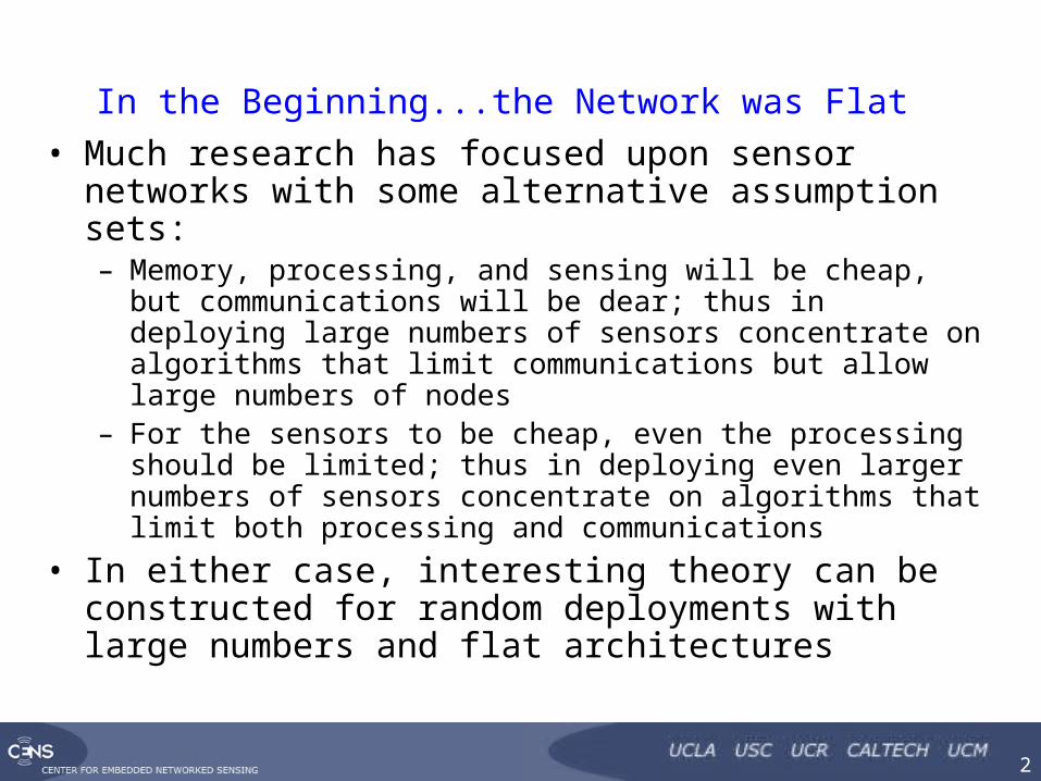
In the Beginning...the Network was Flat

• Much research has focused upon sensor networks with some alternative assumption sets:– Memory, processing, and sensing will be cheap, but

communications will be dear; thus in deploying large numbers of sensors concentrate on algorithms that limit communications but allow large numbers of nodes

– For the sensors to be cheap, even the processing should be limited; thus in deploying even larger numbers of sensors concentrate on algorithms that limit both processing and communications

• In either case, interesting theory can be constructed for random deployments with large numbers and flat architectures


3

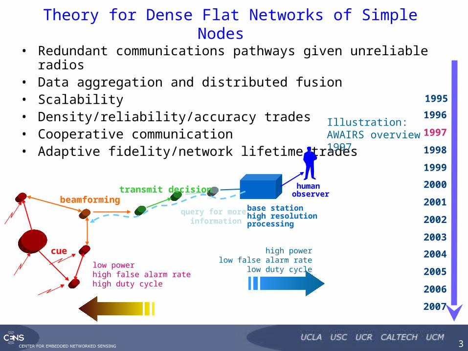
Theory for Dense Flat Networks of Simple Nodes

• Redundant communications pathways given unreliable radios• Data aggregation and distributed fusion• Scalability• Density/reliability/accuracy trades• Cooperative communication• Adaptive fidelity/network lifetime trades

human observer

low powerhigh false alarm ratehigh duty cycle

beamformingtransmit decision

query for more information

base stationhigh resolutionprocessing

cue high powerlow false alarm rate

low duty cycle

Illustration:AWAIRS overview1997

1996

1997

1998

1999

2000

2001

2002

2003

2004

2005

2006

2007

1995


4

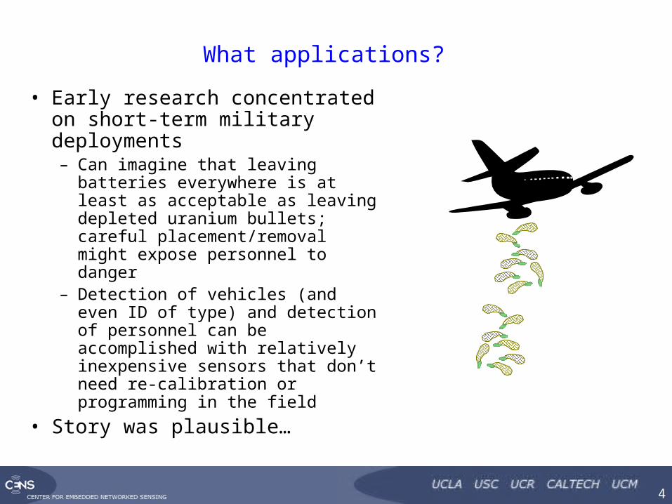
What applications?

• Early research concentrated on short-term military deployments– Can imagine that leaving batteries

everywhere is at least as acceptable as leaving depleted uranium bullets; careful placement/removal might expose personnel to danger

– Detection of vehicles (and even ID of type) and detection of personnel can be accomplished with relatively inexpensive sensors that don’t need re-calibration or programming in the field

• Story was plausible…


5

But was this ever done?

• Military surveillance– Largest outdoor deployment (10000 nodes or so) was hierarchical

and required careful placement; major issues with radio propagation even on flat terrain

– Vehicles are relatively easy to detect with aerial assets, and the major problem with personnel is establishment of intent; this requires a sequence of images

– The major challenge is urban operations, which demands much longer-term monitoring as well as concealment

• Science applications diverge even more in basic requirements– Scientists want to know precisely where things are; cannot leave

heavy metals behind; many other issues

• Will still want dense networks of simple nodes in some locations, but will be system component


6

Practical Design Constraints

• Validation (=debugging) is usually very painful– One part design, 1000 parts testing– Never exhaustively test with the most reliable method

• So how can we trust the result given all the uncertainties?– Not completely, so the design process deliberately minimizes the

uncertainties through re-use of trusted components

• But is the resulting modular model/design efficient?– Fortunately not for academics; one can always propose a more

efficient but untestable design

• Our goal: building systems for sequence of deployments that evolve with user goals


7

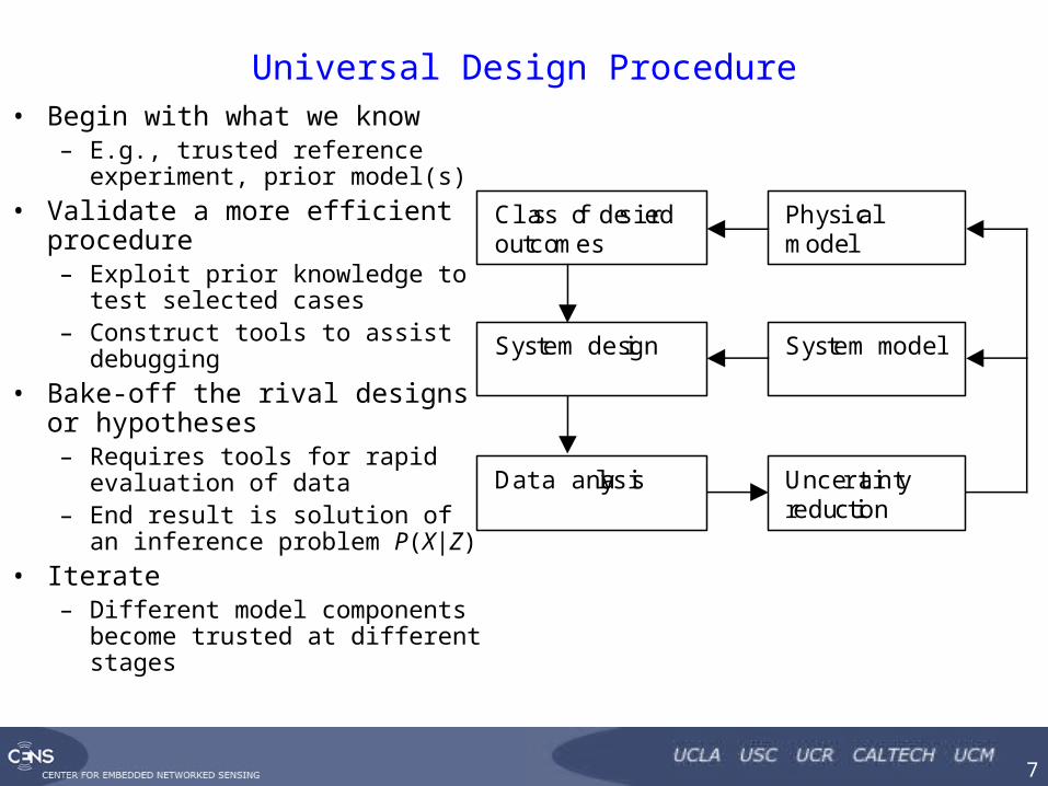
Universal Design Procedure• Begin with what we know

– E.g., trusted reference experiment, prior model(s)

• Validate a more efficient procedure– Exploit prior knowledge to test

selected cases– Construct tools to assist

debugging

• Bake-off the rival designs or hypotheses– Requires tools for rapid

evaluation of data– End result is solution of an

inference problem P(X|Z)

• Iterate– Different model components

become trusted at different stages

Class of desiredoutcomes

Physicalmodel

System design System model

Data analysis Uncertaintyreduction


8

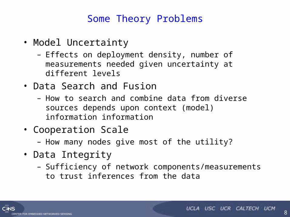
Some Theory Problems

• Model Uncertainty– Effects on deployment density, number of measurements

needed given uncertainty at different levels

• Data Search and Fusion– How to search and combine data from diverse sources

depends upon context (model) information information

• Cooperation Scale– How many nodes give most of the utility?

• Data Integrity– Sufficiency of network components/measurements to trust

inferences from the data


9

Sampling Density, Model, and Objectives

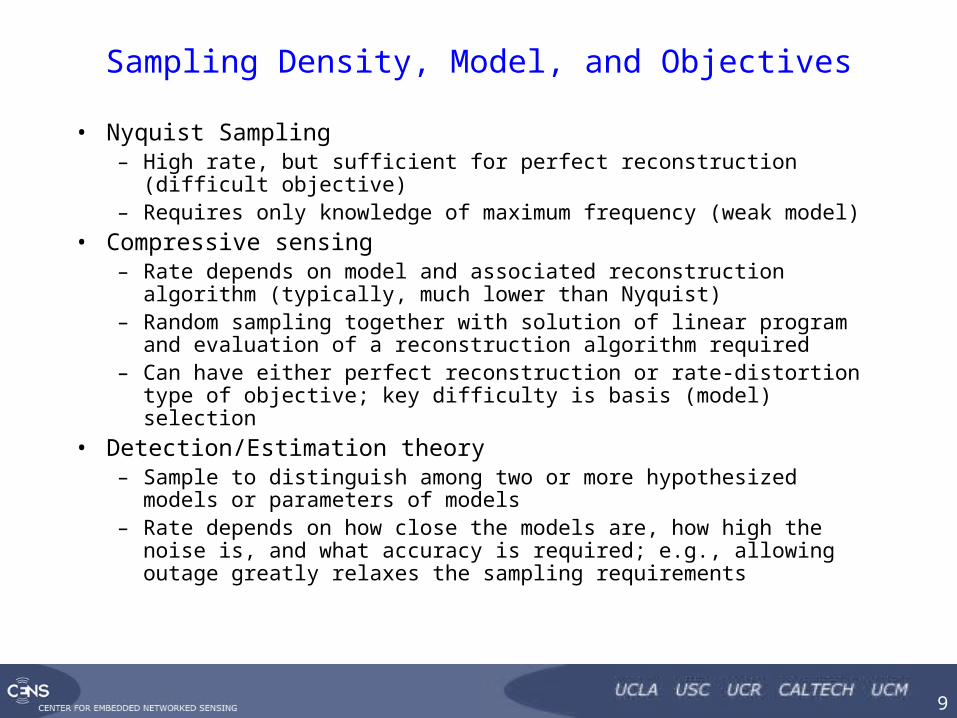
• Nyquist Sampling– High rate, but sufficient for perfect reconstruction (difficult objective)– Requires only knowledge of maximum frequency (weak model)

• Compressive sensing– Rate depends on model and associated reconstruction algorithm

(typically, much lower than Nyquist)– Random sampling together with solution of linear program and

evaluation of a reconstruction algorithm required– Can have either perfect reconstruction or rate-distortion type of

objective; key difficulty is basis (model) selection

• Detection/Estimation theory– Sample to distinguish among two or more hypothesized models or

parameters of models– Rate depends on how close the models are, how high the noise is,

and what accuracy is required; e.g., allowing outage greatly relaxes the sampling requirements


10

Some Tradeoffs

• Sampling Density vs. Cooperation Scale– Distributed algorithms for reconstruction or estimation usually pay

only a small density penalty, with massive computational and communications reduction

• Sampling Density vs. Model Certainty– Model knowledge has huge impact on sampling density– However, within compressive sensing regime not clear that finding

“best” model is worth the effort compared to finding “good” ones

• Sampling Density vs. Measurement Accuracy– Our results suggest relatively modest increase in density is

sufficient to deal with faulty sensors– Low accuracy pays large density price; tradeoff similar to sigma-

delta A/D

• Sampling Density vs. Difficulty of Objective– Reduced fidelity of reconstruction, allowance of outages, etc. can

vastly reduce the number of samples required


11

Search and Fusion• Utility of data depends upon context

– That is, what modeling assumptions are made in its collection– “Raw” data always involves some model for the transducer, and

usually compensation for confounding factors– Cannot attach certainty to measurements without this– More context information improves the ability for the data to be

used for multiple purposes

• Search is conducted on context information or model parameters– Data volume is too large, and data is meaningless without context– Instead search on identifying tags, either separately supplied or

derived through signal processing associated with a model

• Conflicting standards make fusion difficult– Standards are usually domain (or agency) specific– Huge variability in the models used for creation of context

information


12

Cooperation Scale: Localization algorithm behavior

In a localization scenario, onlya handful of sensors more thanminimum required yield most ofthe utility.More doesn’t really help thatmuch.

This behavior depends on the utility from the sensor. Does this happen often?


13

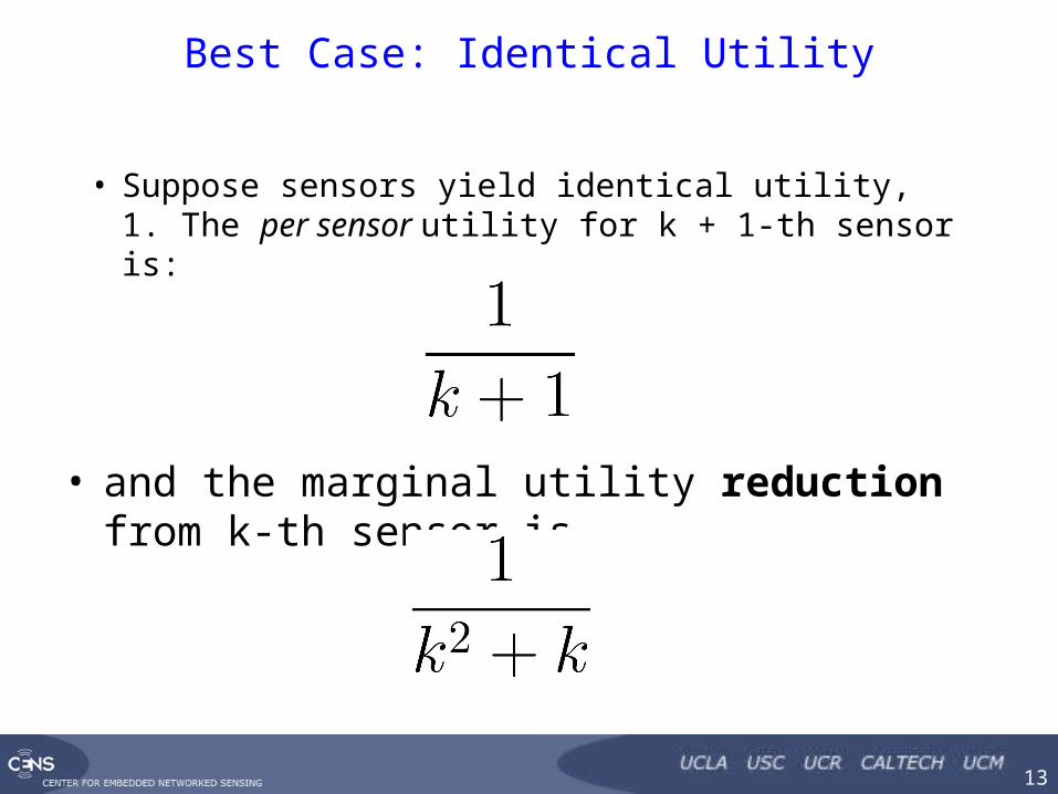
Best Case: Identical Utility

• Suppose sensors yield identical utility, 1. The per sensor utility for k + 1-th sensor is:

• and the marginal utility reduction from k-th sensor is


14

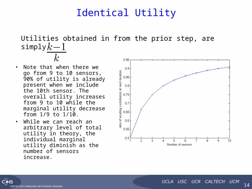
Identical Utility

• Note that when there we go from 9 to 10 sensors, 90% of utility is already present when we include the 10th sensor. The overall utility increases from 9 to 10 while the marginal utility decrease from 1/9 to 1/10.

• While we can reach an arbitrary level of total utility in theory, the individual marginal utility diminish as the number of sensors increase.

Utilities obtained in from the prior step, aresimply


15

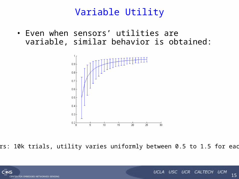
Variable Utility

• Even when sensors’ utilities are variable, similar behavior is obtained:

Parameters: 10k trials, utility varies uniformly between 0.5 to 1.5 for each sensor.


16

Order Statistics

• When we draw n random variables, what is the distribution for the k-th smallest within the n variables?

• Order statistics answer this type of question. For the n-th IID random variable, each drawn according to fR(r), the order statistic for the k-th random variable is


17

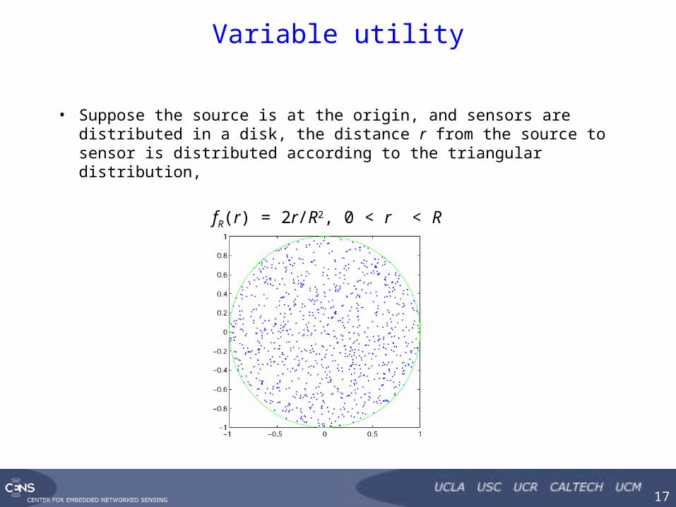
Variable utility

• Suppose the source is at the origin, and sensors are distributed in a disk, the distance r from the source to sensor is distributed according to the triangular distribution,

fR(r) = 2r/R2, 0 < r < R


18

Variable utility, disk

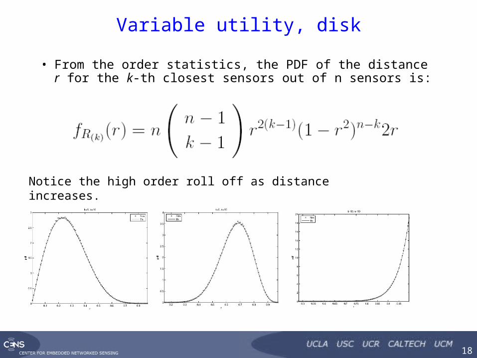
• From the order statistics, the PDF of the distance r for the k-th closest sensors out of n sensors is:

Notice the high order roll off as distance increases.


19

Variable utility, disk 2

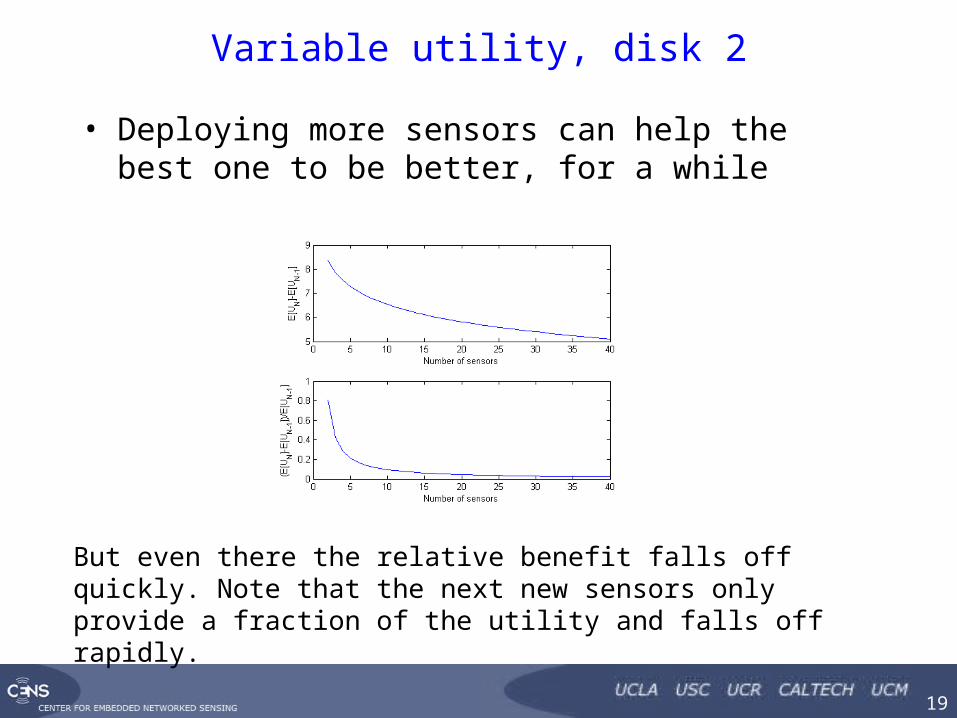
• Deploying more sensors can help the best one to be better, for a while

But even there the relative benefit falls off quickly. Note that the next new sensors only provide a fraction of the utility and falls off rapidly.


20

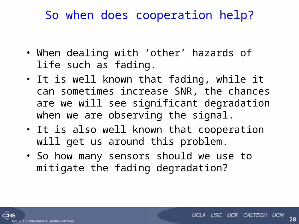
So when does cooperation help?

• When dealing with ‘other’ hazards of life such as fading.

• It is well known that fading, while it can sometimes increase SNR, the chances are we will see significant degradation when we are observing the signal.

• It is also well known that cooperation will get us around this problem.

• So how many sensors should we use to mitigate the fading degradation?


21

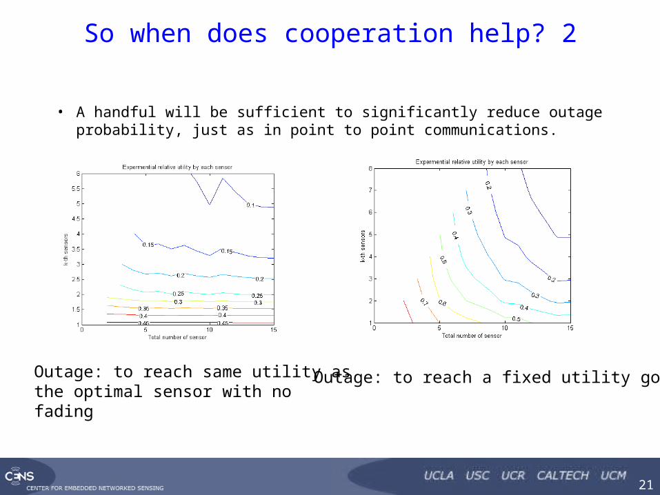
So when does cooperation help? 2

• A handful will be sufficient to significantly reduce outage probability, just as in point to point communications.

Outage: to reach same utility as the optimal sensor with no fading

Outage: to reach a fixed utility goal


22

Asymptotic Considerations

• What happens when we have a large number of sensors?

• There are large variety of configurations possible, but we will assume the following– Source at origin, and sensors surrounding it– Constant deployment density (additional sensors are placed

further away from the source)– All sensors have identical statistical performance, and differ

only by their distances– Coherent combining possible (i.e. Maximal Ratio Combining,

MRC), e.g., for a detection problem


23

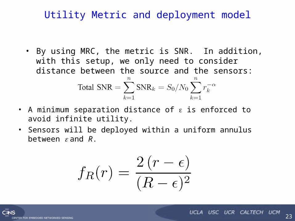
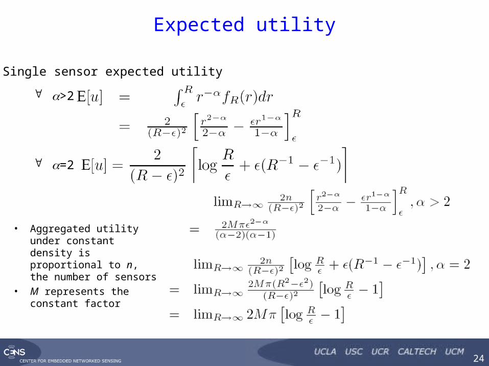
Utility Metric and deployment model

• By using MRC, the metric is SNR. In addition, with this setup, we only need to consider distance between the source and the sensors:

• A minimum separation distance of is enforced to avoid infinite utility.

• Sensors will be deployed within a uniform annulus between and R.


24

Expected utility

>2

=2

• Aggregated utility under constant density is proportional to n, the number of sensors

• M represents the constant factor

Single sensor expected utility


25

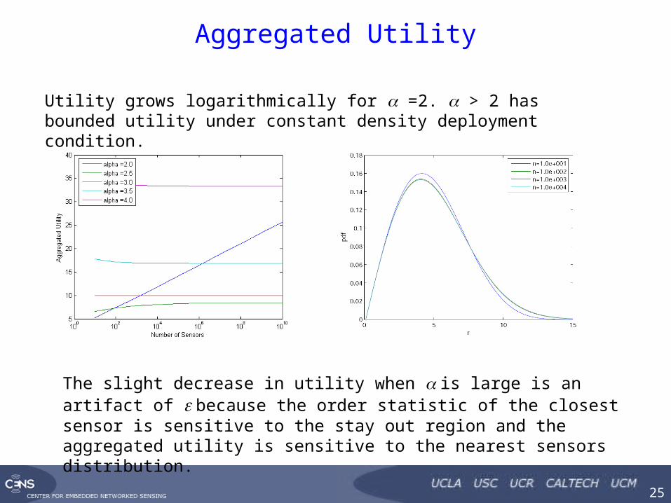
Aggregated Utility

Utility grows logarithmically for =2. > 2 has bounded utility under constant density deployment condition.

The slight decrease in utility when is large is an artifact of because the order statistic of the closest sensor is sensitive to the stay out region and the aggregated utility is sensitive to the nearest sensors distribution.


26

Conclusion: Localization Problem

• Utilities are dominated by the few that have the most utility.

• For the purpose of estimation, a large number of sensors help a priori by placing a sensor closer to the source, but will not help during the estimation process after the sensors were placed and the event of interest is taking place.

• Under constant density, even with a large number of sensors, cooperation is not helpful in significantly increasing the aggregated utility.


27

Other Cooperation Problems

• Examination of other utility functions– How broad is the class of problems to which our basic

conclusions apply?

• Examination of related problems– Quantized observations– Tracking– Estimation of continuous phenomena (e.g., fields) or

extraction of statistics– Coverage


28

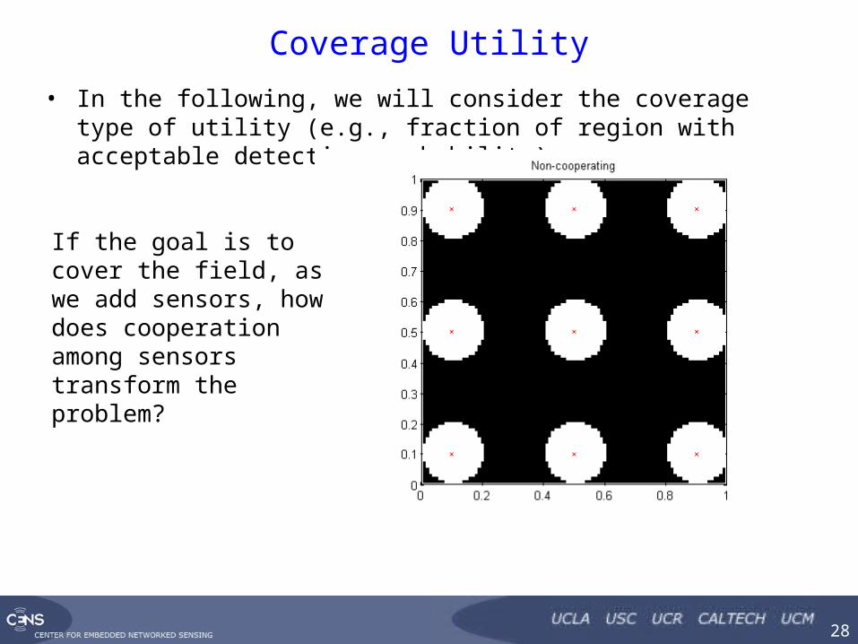
Coverage Utility

• In the following, we will consider the coverage type of utility (e.g., fraction of region with acceptable detection probability).

If the goal is to cover the field, as we add sensors, how does cooperation among sensors transform the problem?


29

Coverage Utility, 2

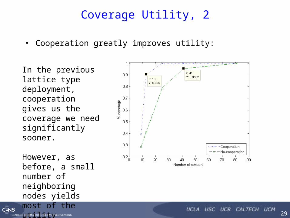
• Cooperation greatly improves utility:

In the previous lattice type deployment, cooperation gives us the coverage we need significantly sooner.

However, as before, a small number of neighboring nodes yields most of the utility


30

Another Reason to Cooperate: Data Integrity

• Sensors are exposed to harsh environments.• This leads to failures or malfunctions in sensors.• Many deployments have had to discard data due to

faulty data:– While examining the micro-climate over the volume of a

redwood tree, only 49% of the data could be used. [TPS05]– A deployment at Great Duck Island classified 3%-60% of data

as faulty [SMP04]

30


31

Sensor Faults

• Faulty data leads to uncertain scientific inferences• Goal is to reliably identify faults as they occur so that we

can immediately take action to either repair or replace sensors.

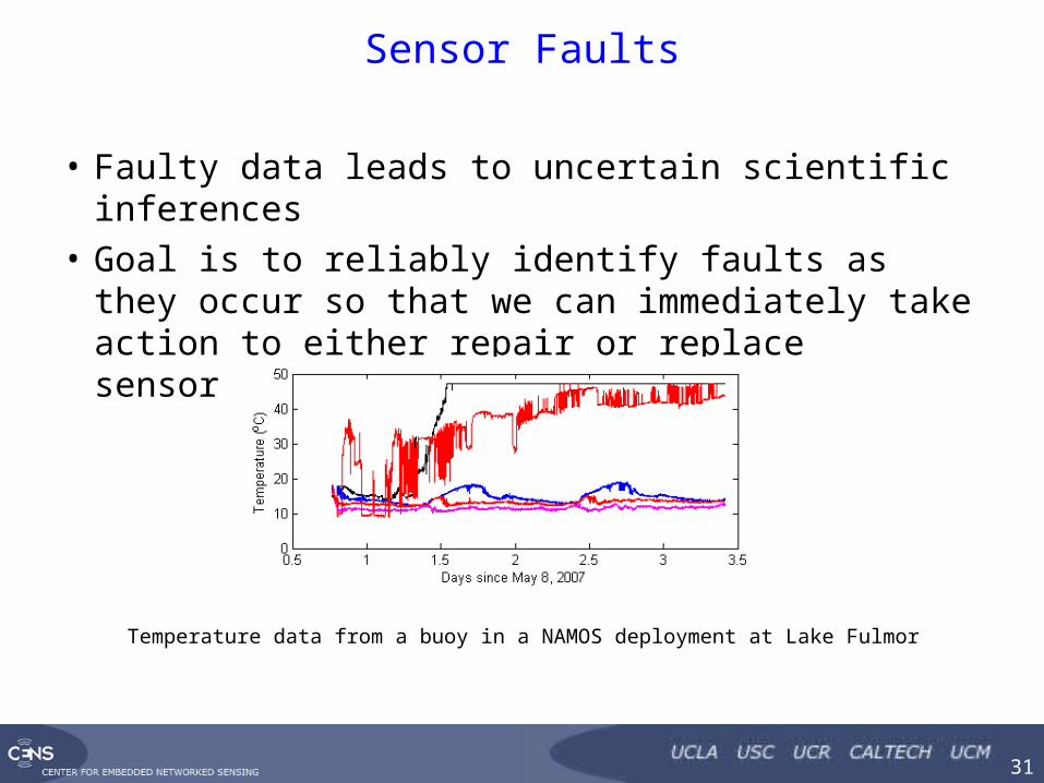
Temperature data from a buoy in a NAMOS deployment at Lake Fulmor


32

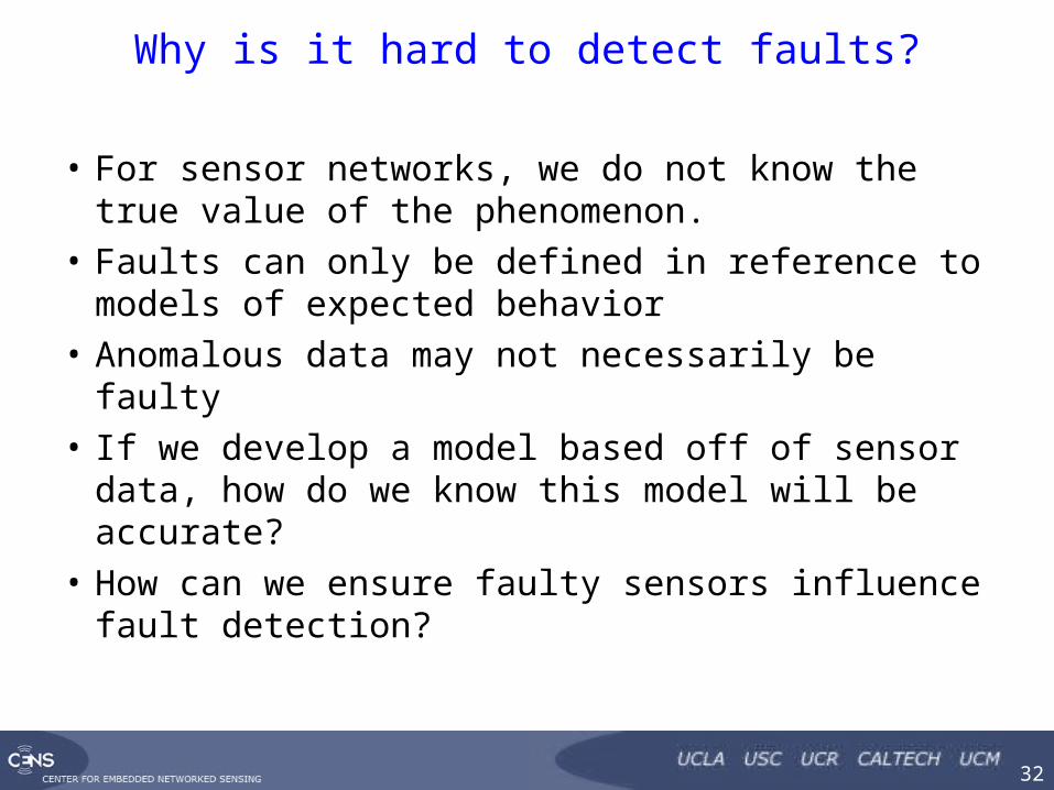
Why is it hard to detect faults?

• For sensor networks, we do not know the true value of the phenomenon.

• Faults can only be defined in reference to models of expected behavior

• Anomalous data may not necessarily be faulty• If we develop a model based off of sensor data, how do

we know this model will be accurate?• How can we ensure faulty sensors influence fault

detection?


33

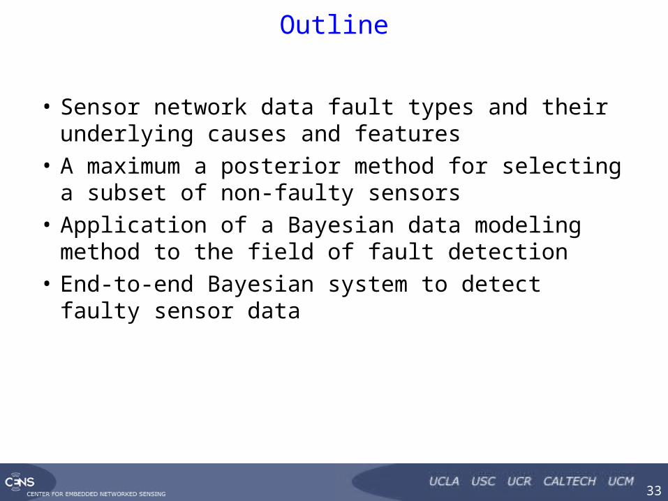
Outline

• Sensor network data fault types and their underlying causes and features

• A maximum a posterior method for selecting a subset of non-faulty sensors

• Application of a Bayesian data modeling method to the field of fault detection

• End-to-end Bayesian system to detect faulty sensor data


34

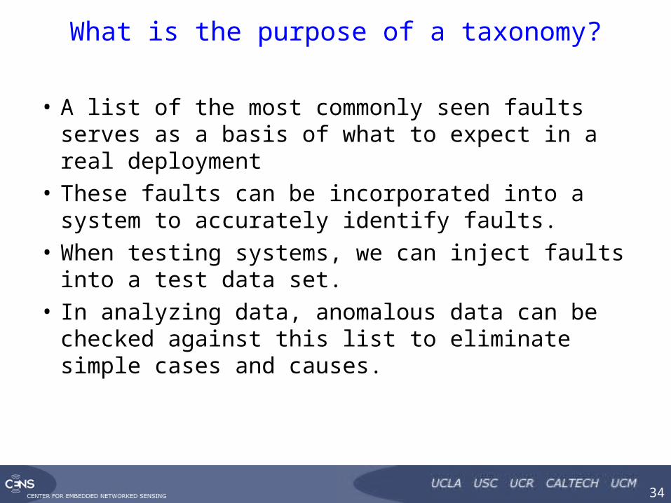
What is the purpose of a taxonomy?

• A list of the most commonly seen faults serves as a basis of what to expect in a real deployment

• These faults can be incorporated into a system to accurately identify faults.

• When testing systems, we can inject faults into a test data set.

• In analyzing data, anomalous data can be checked against this list to eliminate simple cases and causes.


35

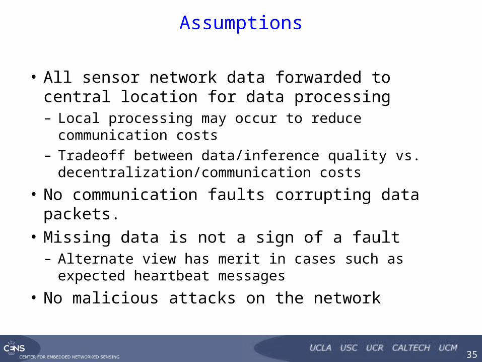
Assumptions

• All sensor network data forwarded to central location for data processing– Local processing may occur to reduce communication costs– Tradeoff between data/inference quality vs.

decentralization/communication costs

• No communication faults corrupting data packets.• Missing data is not a sign of a fault

– Alternate view has merit in cases such as expected heartbeat messages

• No malicious attacks on the network


36

Data Modeling

• Models are mathematical representations of expected behavior for both non-faulty and faulty data.– Can be defined as a range of values:

• Relative humidity is between 0% and 100%

• Temperature is greater than 0K

– Can be a well defined formulaic model that can generate simulated data:• Temperature = A * time + B.

• In the absence of ground truth, faults can only be defined by models of expected behavior

• Human input necessary for modeling and updates by providing vital contextual knowledge.


37

Sensor network features

• Features – describes data, system or environment useful in fault detection

• Used to detect or explain the cause of faults• Aids in systematically defining faults.• Three classes of features:

– Environment features: sensor location, rainy weather, microclimate models

– System features: sensor transducer/ADC performance, sensor age, battery state, noise

– Data features: mean/variance, correlation, gradient


38

Sensor Network Data Faults

• Faults have varying levels of importance dependent on context:– Some still hold informational value and can be used to make

inferences at lower fidelity– Some are totally uninterpretable and must be discarded

• Two overlapping approaches to defining a fault– “Data-centric” view: describe faults by characteristics of the

data behavior– “System” view: define a physical malfunction with a sensor and

describe what type of features this will exhibit in the data

• Multiple faults may occur at the same time and may be related


39

Data-centric view

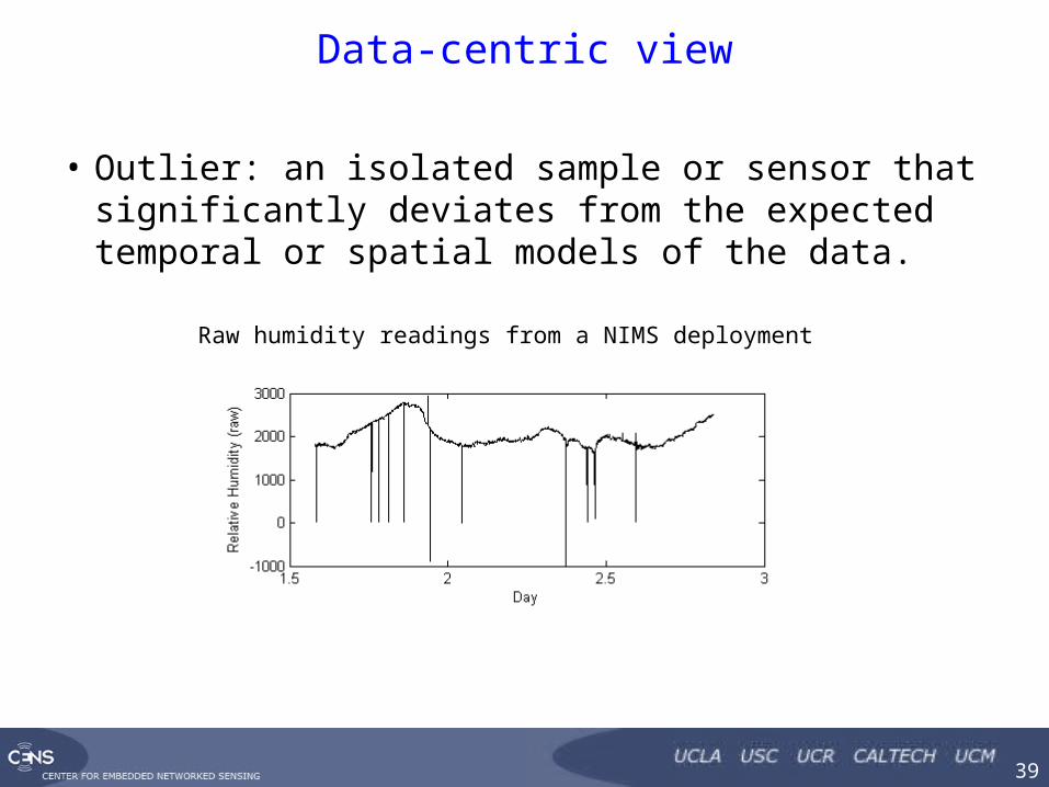
• Outlier: an isolated sample or sensor that significantly deviates from the expected temporal or spatial models of the data.

Raw humidity readings from a NIMS deployment


40

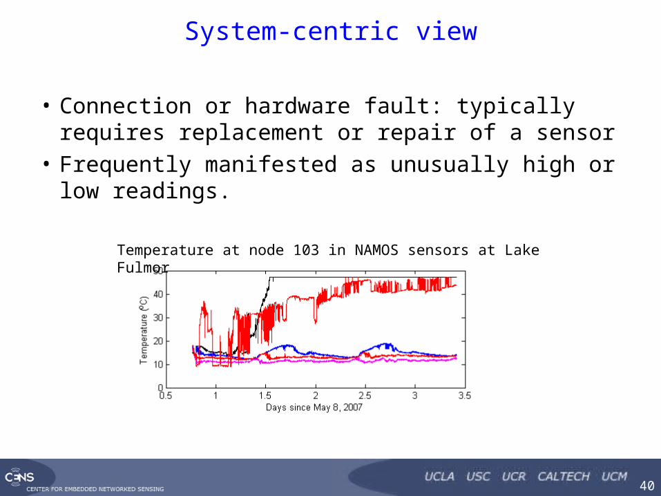
System-centric view

• Connection or hardware fault: typically requires replacement or repair of a sensor

• Frequently manifested as unusually high or low readings.

Temperature at node 103 in NAMOS sensors at Lake Fulmor


41

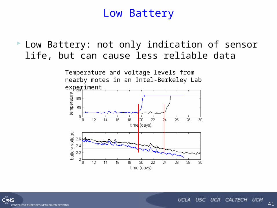
Low Battery

Low Battery: not only indication of sensor life, but can cause less reliable data

Temperature and voltage levels from nearby motes in an Intel-Berkeley Lab experiment


42

Design Principles

• Sensor network fault detection design principles:– We must model or restrict ourselves to a model of the

phenomenon we are sensing– Based upon this model, we must determine the expected behavior

of the data using available data– We must determine when sensor data conforms to the expected

behavior of the network or phenomenon– We must remedy problems or classify behavior as either

acceptable or faulty and update our models


43

Online fault detection algorithm

• First develop an online fault detection system with immediate decisions.

• Two phase system:– Bayesian maximum a posteriori selection of a subset of

agreeing sensors which are used to model the expected phenomenon behavior

– Judgment of fault or non-fault based upon this expected behavior.


44

Additional Assumptions

• First assume sensors will have the same trends (slopes).– Later will further restrict to all sensors measuring the same

values.

• Non-faulty data is locally linear.• No large data gaps• Gaussian noise model for simplicity• At least sensors are not faulty at any given time


45

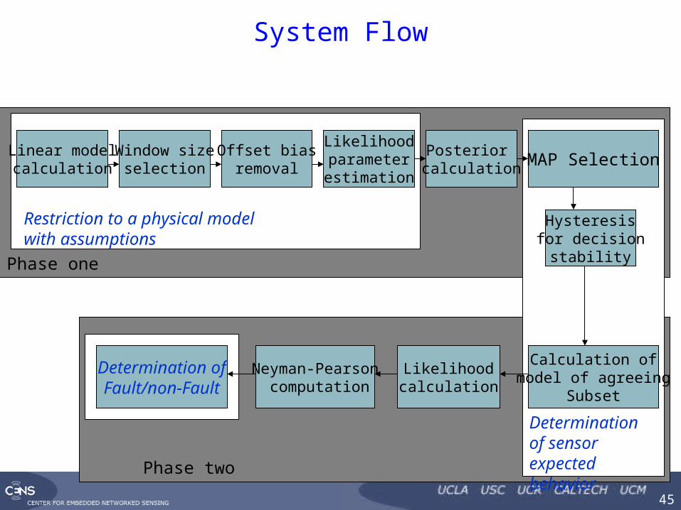
System Flow

Calculation ofmodel of agreeing

Subset

Determination ofFault/non-Fault

MAP Selection

Hysteresisfor decision

stability

Window sizeselection

Offset biasremoval

Posterior calculation

Linear modelcalculation

Likelihoodparameterestimation

Likelihoodcalculation

Phase one

Phase two

Restriction to a physical model with assumptions

Determination of sensor expected behavior

Neyman-Pearson computation


46

Results

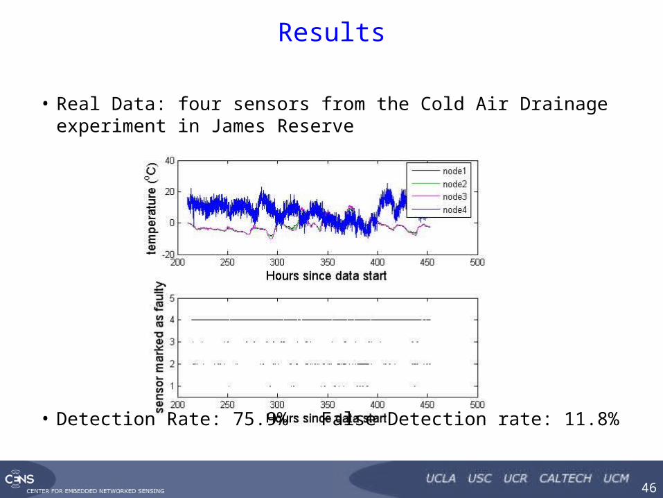
• Real Data: four sensors from the Cold Air Drainage experiment in James Reserve

• Detection Rate: 75.9% False Detection rate: 11.8%


47

Hierarchical Bayesian space-time (HBST) modeling

• Introduce a new modeling technique that is more capable of representing sensor network data.

• Utilize the HBST modeling approach of [WBC98] and adapt it for fault detection.

• Not perfect but more accurate and more robust than linear AR modeling


48

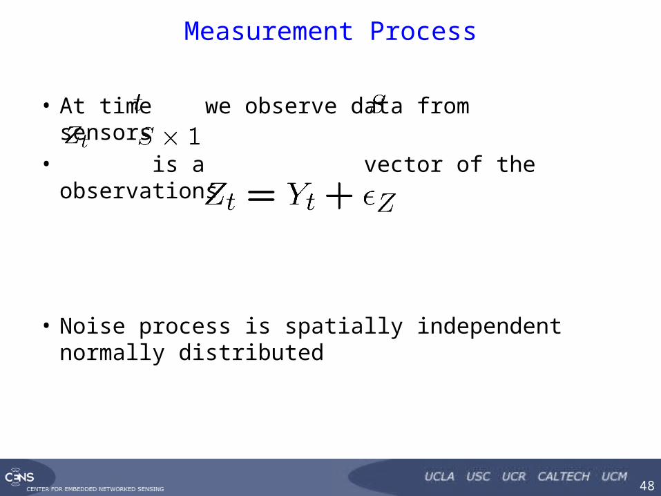
Measurement Process

• At time we observe data from sensors• is a vector of the observations

• Noise process is spatially independent normally distributed


49

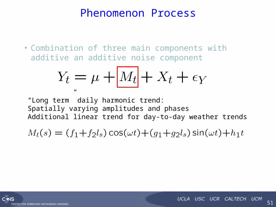
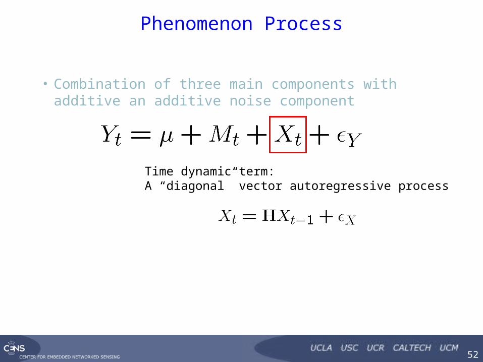
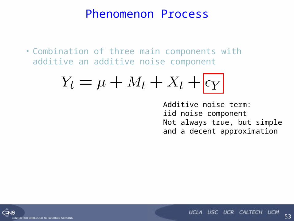
Phenomenon Process

• Combination of three main components with additive an additive noise component


50

Phenomenon Process


Site specific mean vector:A first order linear regression assumes sitespecific mean has a linear trend in space.


51

Phenomenon Process


“Long term” daily harmonic trend:Spatially varying amplitudes and phasesAdditional linear trend for day-to-day weather trends


52

Phenomenon Process


Time dynamic term:A “diagonal” vector autoregressive process


53

Phenomenon Process


Additive noise term:iid noise componentNot always true, but simple and a decent approximation


54

Model Simulation

• Additionally the noise components , , are given prior inverse gamma distributions

• We use Gibbs sampling to simulate draws from the posterior distribution, , where is a vector of all parameters being modeled.

• Gibbs sampling allows for quick and easy computation of samples from the full posterior distribution using easier to sample conditional distributions.

• Result is a number of random draws for each of the parameters in Yt as well as draws for Xt


55

Fault Detection

• Gibbs sampling is computationally expensive• Semi-realtime detection system.

– Calculate at a regular interval at a time scale larger than the sensing interval, e.g. once a day for 5 minute sampling interval

• To test the abilities of HBST modeling we introduce a simplistic thresholding technique to detect behaviors outside the expected range.

• We compare against a similar thresholding technique that uses linear AR modeling

• For all of our calculations, we use the sample mean across all sample draws from the simulated posteriors


56

Results: Goal

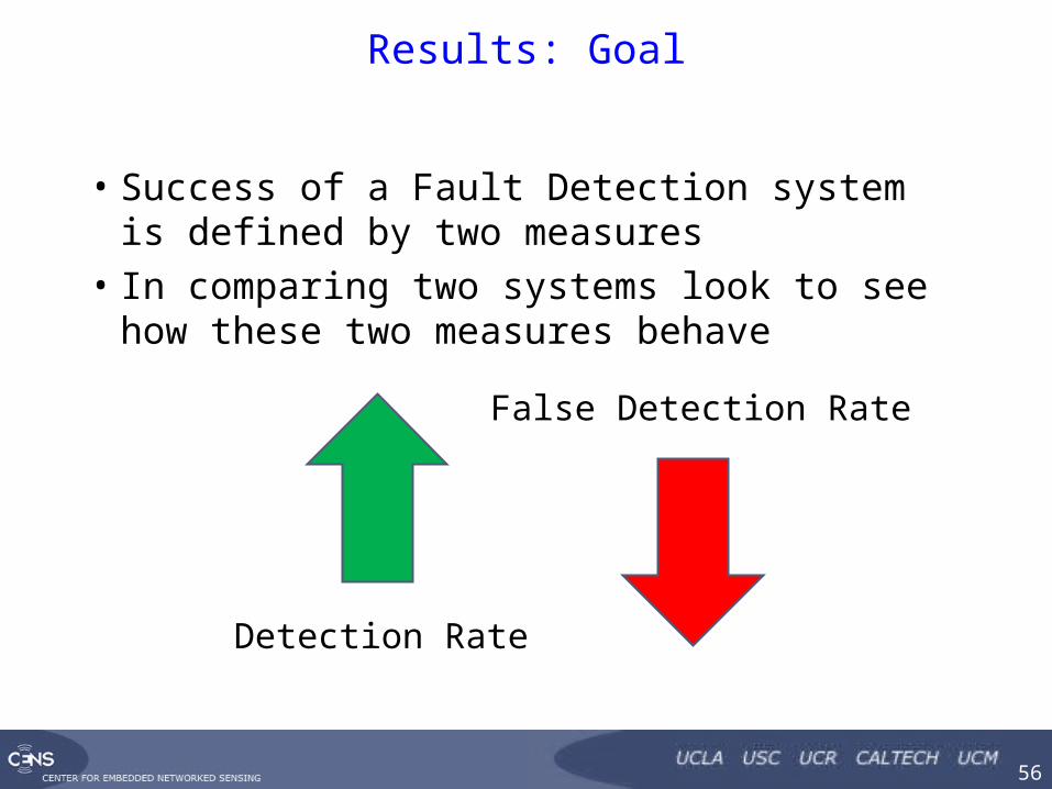
• Success of a Fault Detection system is defined by two measures

• In comparing two systems look to see how these two measures behave

Detection Rate

False Detection Rate


57

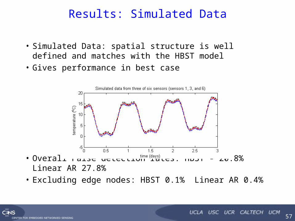
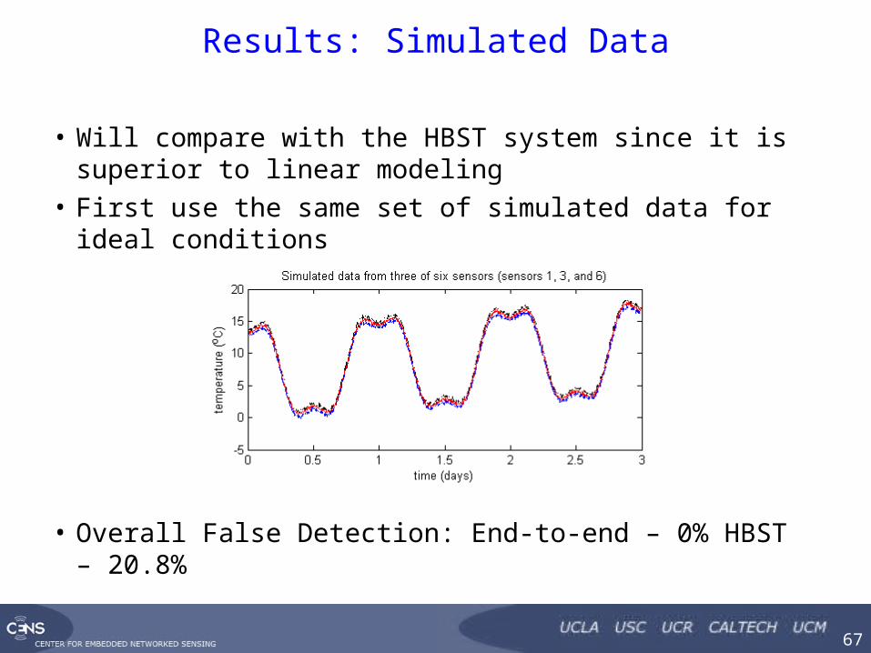
Results: Simulated Data

• Simulated Data: spatial structure is well defined and matches with the HBST model

• Gives performance in best case

• Overall False detection rates: HBST - 20.8% Linear AR 27.8%

• Excluding edge nodes: HBST 0.1% Linear AR 0.4%


58

Results: Cold Air Drainage

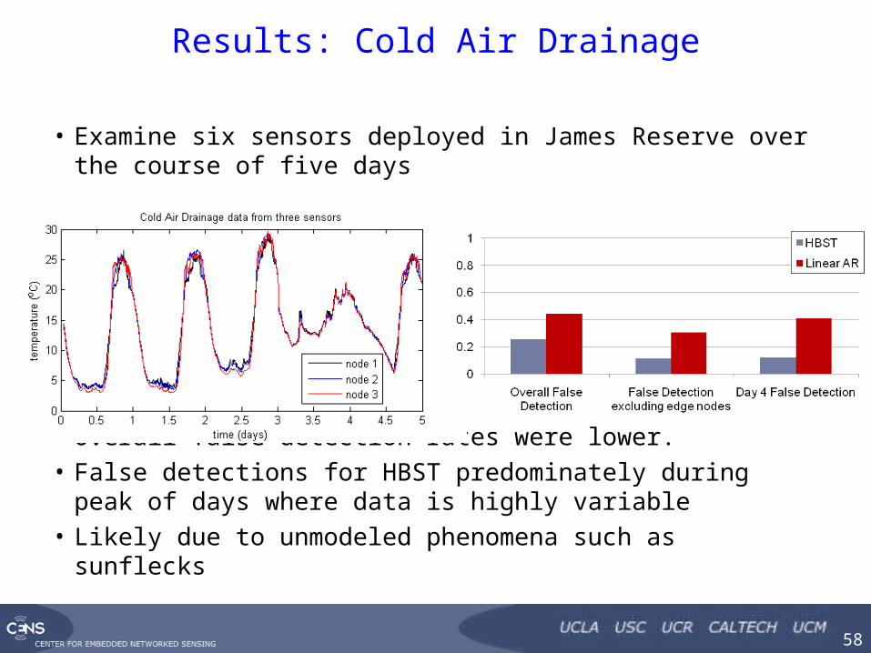
• Examine six sensors deployed in James Reserve over the course of five days

• Overall false detection rates were lower.• False detections for HBST predominately during peak of

days where data is highly variable• Likely due to unmodeled phenomena such as sunflecks


59

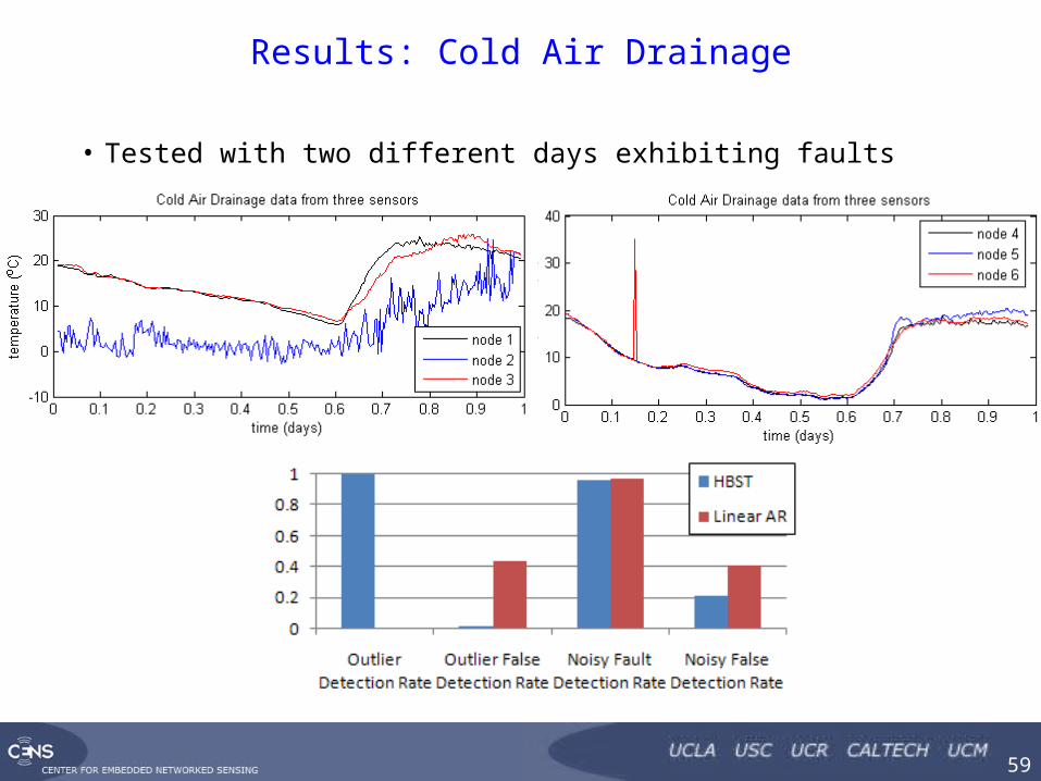
Results: Cold Air Drainage

• Tested with two different days exhibiting faults


60

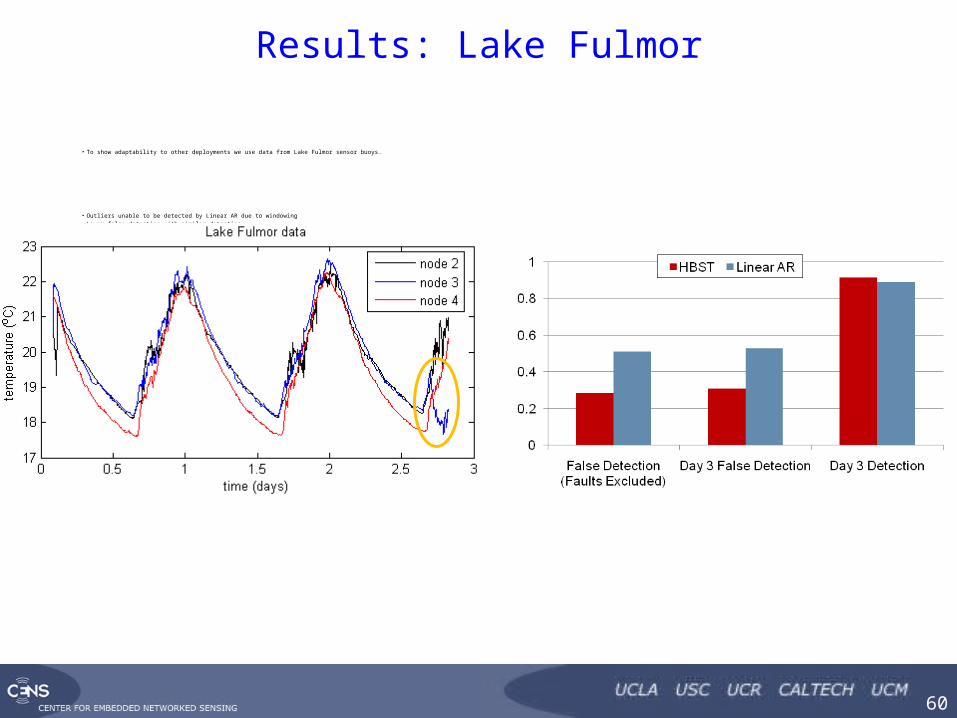
Results: Lake Fulmor

• To show adaptability to other deployments we use data from Lake Fulmor sensor buoys.

• Outliers unable to be detected by Linear AR due to windowing• Lower false detection with similar detection


61

Putting It All Together

• Introduced a method to select the most similar sensors based on a MAP selection

• But the modeling was inaccurate

• Introduced a more accurate modeling approach, HBST.• But the fault detection scheme was overly simplistic

• Combine the two to get the best of both worlds


62

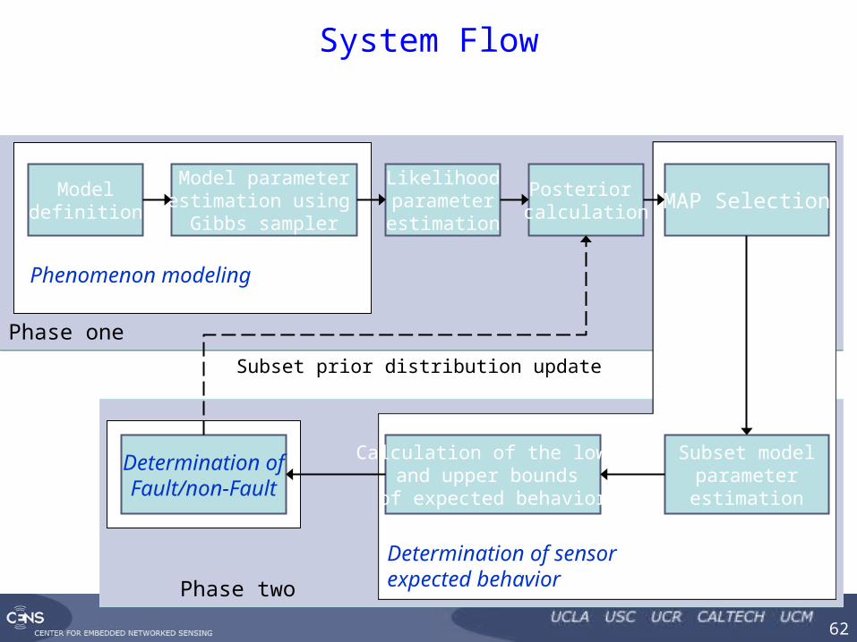
System Flow

Subset modelparameterestimation

Determination ofFault/non-Fault

MAP SelectionModel parameterestimation using

Gibbs sampler

Posterior calculation

Modeldefinition

Likelihoodparameterestimation

Calculation of the lowerand upper bounds

of expected behavior

Phase one

Phase two

Phenomenon modeling

Determination of sensor expected behavior

Subset prior distribution update


63

Phase One

• First we model the phenomenon using all of the sensors using the method previously described

• We again use the time dynamic term to assess the agreement among a sensor subset

• Use subsets of size to establish clear majorities of agreement

• For each time instant and subset we can calculate the posterior density

• The best subset is then:


64

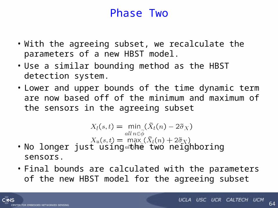
Phase Two

• With the agreeing subset, we recalculate the parameters of a new HBST model.

• Use a similar bounding method as the HBST detection system.

• Lower and upper bounds of the time dynamic term are now based off of the minimum and maximum of the sensors in the agreeing subset

• No longer just using the two neighboring sensors.• Final bounds are calculated with the parameters of the

new HBST model for the agreeing subset


65

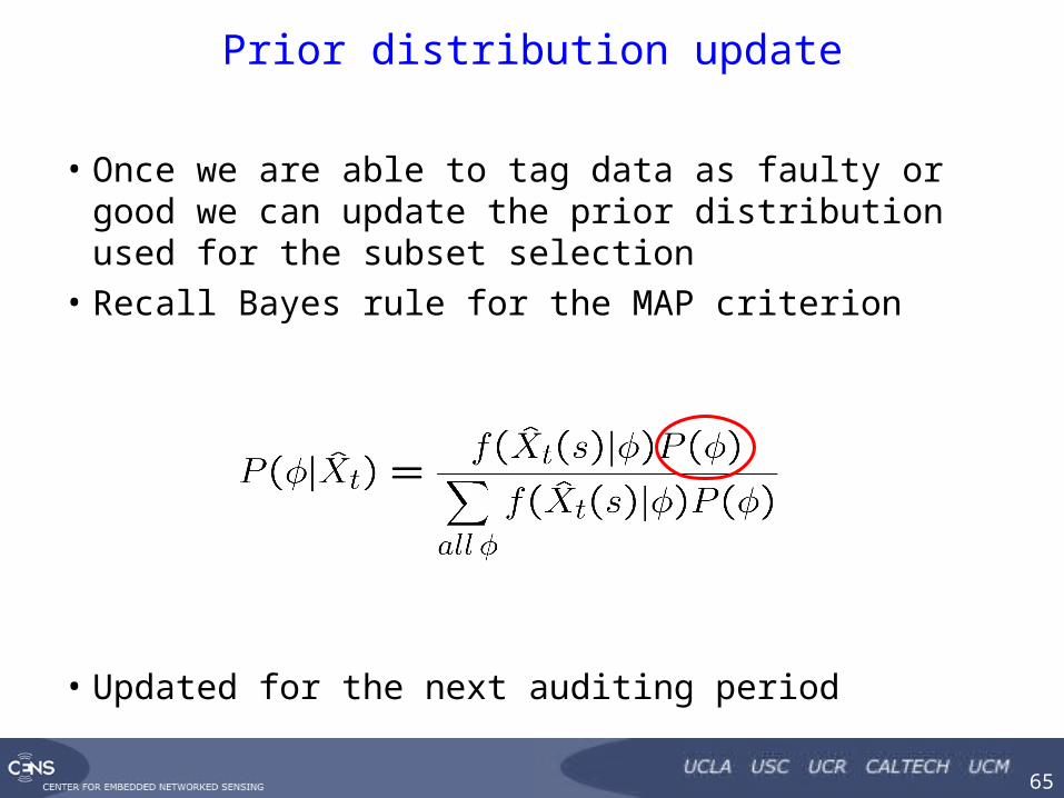
Prior distribution update

• Once we are able to tag data as faulty or good we can update the prior distribution used for the subset selection

• Recall Bayes rule for the MAP criterion

• Updated for the next auditing period


66

Issues Resolved

• By combining the best of the two systems we have resolved some issues from the MAP selection system– Window size selection is no longer a concern since we are

auditing on periods convenient to use (every day)– No need for a lag to maintain decision stability since we are

auditing on convenient periods– No need to remove bias or offset since HBST modeling

includes these inherently

• Issues resolved from the HBST simple tagging system– Use of agreeing subset means no faulty sensor is ever

included in a fault decision– Edge sensors now are judged by more than one other sensor


67

Results: Simulated Data

• Will compare with the HBST system since it is superior to linear modeling

• First use the same set of simulated data for ideal conditions

• Overall False Detection: End-to-end – 0% HBST – 20.8%


68

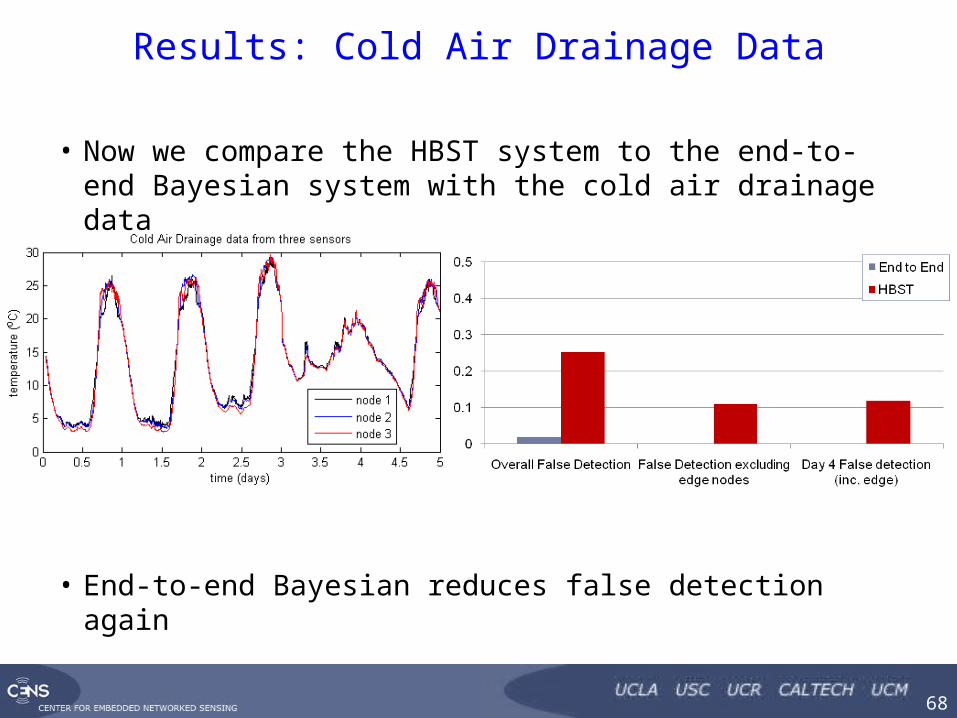
Results: Cold Air Drainage Data

• Now we compare the HBST system to the end-to-end Bayesian system with the cold air drainage data

• End-to-end Bayesian reduces false detection again


69

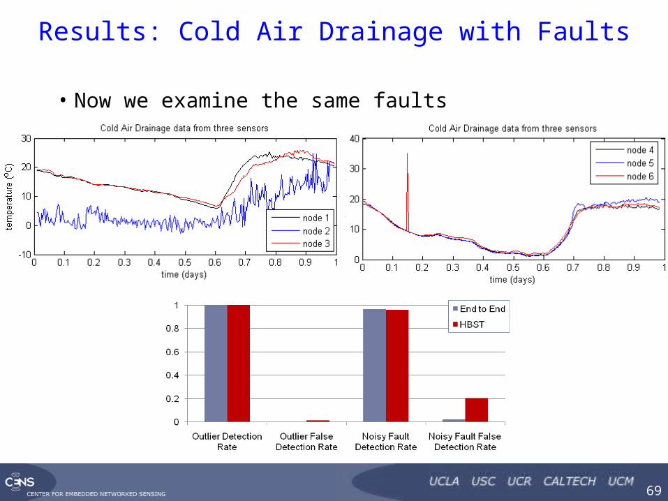
Results: Cold Air Drainage with Faults

• Now we examine the same faults


70

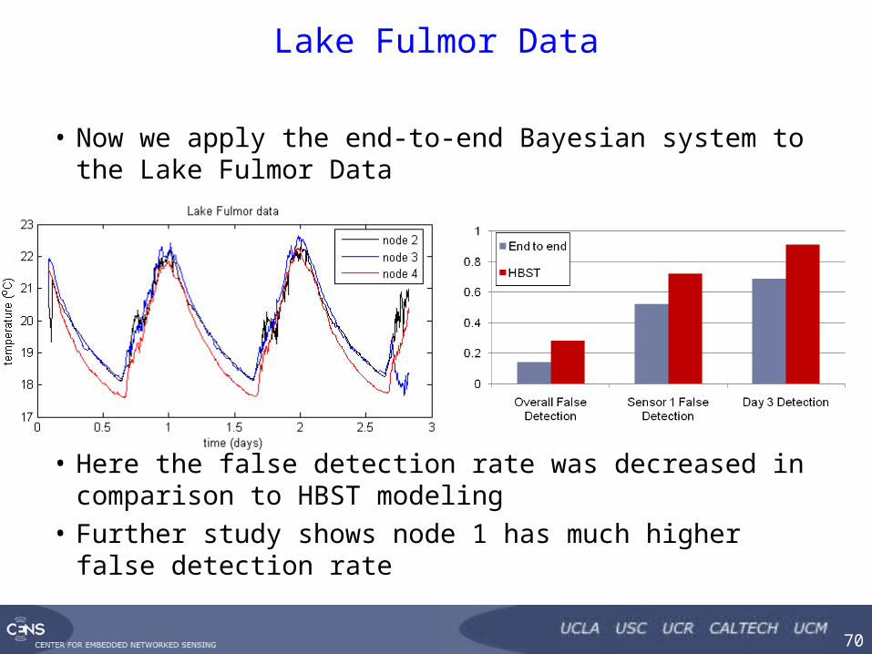
Lake Fulmor Data

• Now we apply the end-to-end Bayesian system to the Lake Fulmor Data

• Here the false detection rate was decreased in comparison to HBST modeling

• Further study shows node 1 has much higher false detection rate


71

Fault Detection Conclusions

• Systematically defined taxonomy of faults

• Developed and implemented a successful fault detection technique using MAP selection and HBST modeling

• Good modeling is important to determining expected behaviors and faults

• Model accuracy and deployment density trade-off– Linear AR modeling may be OK with dense deployments

– Lower deployment requires something accurate modeling like HBST

• Bayesian techniques are amenable to model updates as new data is collected

• Human intervention and monitoring will be required on some level when there is no extensive validation period


72

Conclusions

• Beyond the flat network, there are many difficult problems

• Focus here has been on the problem of reliable inference with minimal resource usage

• Many tradeoffs among model knowledge, sampling density, and inference objectives

center for embedded networked sensing 1 cooperation, sampling and models in sensor network research...

Documents