cen tre for computational geography, school of geography

A comparative study of typologies for rural areas in Europe

DIMITRIS BALLAS,∗ THANASIS KALOGERESIS ⊥ AND LOIS LABRIANIDIS ⊥

Paper submitted to the 43rd European Congress of the Regional Science Association, Jyväskylä, Finland, 27-30 August 2003

∗ Centre for Computational Geography, School of Geography, University of Leeds, Leeds LS2

9JT, UK. Email: [email protected]

⊥ Regional Development and Policy Research Unit (RDPRU), Department of Economic

Sciences, University of Macedonia, 156 Egnatia Street, PO Box 1591, Thessaloniki 54006,

Greece. Emails: [email protected]; [email protected]

Abstract: This paper examines alternative methodologies to build a typology for rural

areas in Europe. First, it reviews the methodologies that have traditionally been used to

construct area typologies in various contexts. It then uses data for European NUTS3

regions to build a typology for rural areas in Europe, on the basis of their peripherality

and rurality. An aggregative approach to building typologies is adopted, under which

the well-established statistical techniques of principal components analysis and cluster

analysis are employed. We then highlight the disadvantages of this approach and we

present an alternative disaggregative approach to the construction of typologies for rural

areas in Europe. Finally, we discuss the policy implications of our suggested typology.

Keywords: rural typologies, rurality, peripherality


Ballas, Kalogeresis and Labrianidis 2

Introduction

This paper presents alternative methodologies for the construction of rural

typologies for European Regions1. The main aim of the research reported in this paper is

to create a typology for rural regions.

At the outset it should be noted that there are several definitions of rural areas.

For instance, despite the limited reliability of quantitative criteria, international

organisations (such as the OECD and EUROSTAT) usually adopt these criteria for the

definition of rural regions as they are particularly useful for inter-regional or inter-state

comparisons. It can be argued that two of the few attributes common to European rural

regions are relatively low population densities and the significant role of agriculture in

the local economy. It is noteworthy that population density has been traditionally used

for the definitions of rural areas in Europe. In particular, at the NUTS52 level rural areas

are defined by EUROSTAT as those with a population density of less than 100

inhabitants per km2. Moreover, according to the EUROSTAT classification, 17.5% of

the total EU population lives in administrative units that belong to rural regions and

cover more than 80% of the total of the EU area. These percentage figures range from

less than 5% in the Netherlands and Belgium to more than 50% in Finland and Sweden.

The OECD distinguishes between three different types of regions on the basis of the

proportion of population living in rural municipalities. In particular, the OECD (1994)

area classification is as follows:

• Predominantly rural areas where more than 50% of the population lives in rural

municipalities.

• Significantly rural areas, where a percentage of 15%-50% of the population lives in

rural municipalities.

• Significantly urban areas, where a percentage of less than 15% of the population

lives in rural municipalities.

The corresponding approach of the EU is based on the degree of urbanisation. In

particular EU regions are classified into 3 different types:

1 This paper has been developed in the context of a research project financed by the EU (Labrianidis et al. 2003).

2 NUTS stands for Nomenclature of Territorial Units for Statistics



1. Densely populated areas, which have a population of more than 50,000 inhabitants

living in contiguous local authority units with a population density of more than 500

inhabitants per km2 (for each local authority).

2. Intermediate areas, which comprise local authority units with population densities of

100 inhabitants per km2 each. The total population of the zone should be more than

50,000 inhabitants, or alternatively, it can be contiguous to a densely populated area.

3. Sparsely populated zones which comprise all the non-densely populated and non-

intermediate EU areas

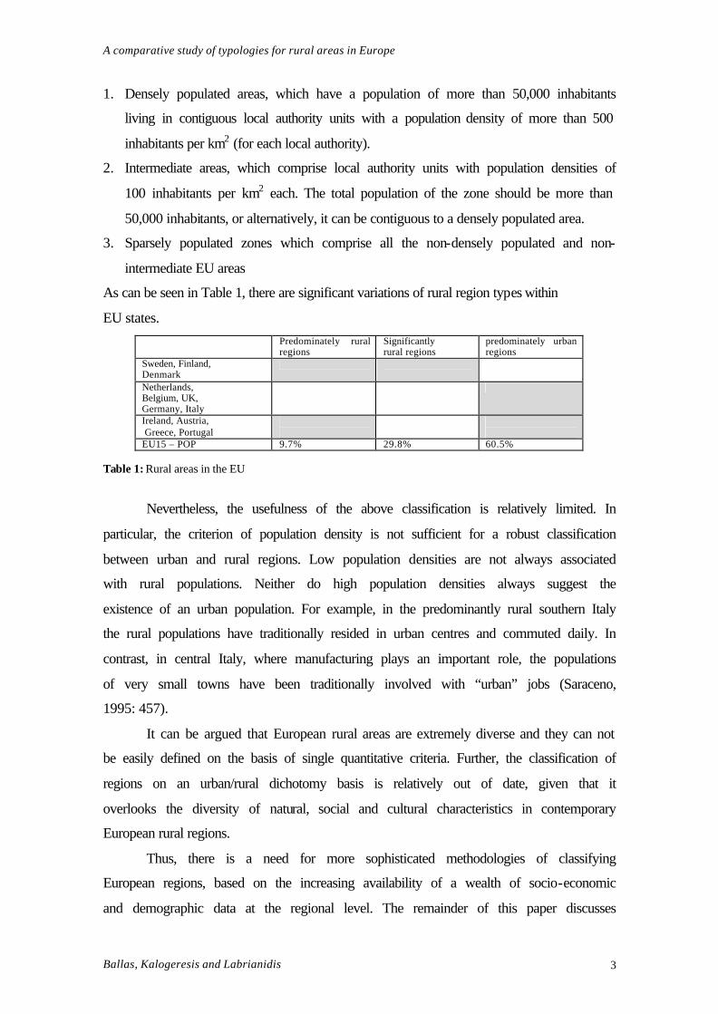
As can be seen in Table 1, there are significant variations of rural region types within

EU states. Predominately rural

regions Significantly rural regions

predominately urban regions

Sweden, Finland, Denmark

Netherlands, Belgium, UK, Germany, Italy

Ireland, Austria, Greece, Portugal

EU15 – POP 9.7% 29.8% 60.5% Table 1: Rural areas in the EU

Nevertheless, the usefulness of the above classification is relatively limited. In

particular, the criterion of population density is not sufficient for a robust classification

between urban and rural regions. Low population densities are not always associated

with rural populations. Neither do high population densities always suggest the

existence of an urban population. For example, in the predominantly rural southern Italy

the rural populations have traditionally resided in urban centres and commuted daily. In

contrast, in central Italy, where manufacturing plays an important role, the populations

of very small towns have been traditionally involved with “urban” jobs (Saraceno,

1995: 457).

It can be argued that European rural areas are extremely diverse and they can not

be easily defined on the basis of single quantitative criteria. Further, the classification of

regions on an urban/rural dichotomy basis is relatively out of date, given that it

overlooks the diversity of natural, social and cultural characteristics in contemporary

European rural regions.

Thus, there is a need for more sophisticated methodologies of classifying

European regions, based on the increasing availability of a wealth of socio-economic

and demographic data at the regional level. The remainder of this paper discusses



different methodologies for the creation of a rural typology for European regions. In

particular, we first discuss past attempts to exploit geographical socio-economic and

demographic databases for the creation of rural typologies. Further, we describe a

geographic database for rural regions that we had at our disposal and shows how we

implemented some of the methodologies described previously to process this database.

In addition, we show how we used statistical cluster analysis techniques to create a

typology on the basis of the processed data. Finally, we present an alternative approach

to creating rural typologies, based on a disaggregative methodology.

Data Issues and Methodological framework

The very essence of the idea to produce a typology of rural areas applicable to

different countries presupposes the definition of a supranational reference framework

preferably based on simple and comparable criteria that are expected to be able to

capture the notion of rurality and peripherality in each rural area. In this section we

review several attempts to create typologies of rural areas, coming from two main

sources. The first one created by OECD (1996)3, while the second is the Rural

Development Typology of European NUTS3 Regions, undertaken in the context of the

Research Programme “Impact of Public Institutions on Lagging Rural and Coastal

Regions” (Copus, 1996), financed by the AIR Project4. The latter is much more

relevant to the research proposed here, as its objective was to ‘create a typology of rural

and coastal desertification in the study regions by using factor analysis and cluster

analysis’ (Copus, 1996, p. 1). Furthermore, it was intended to complement the statistical

profiles by providing a basis on which to ‘benchmark’ the study areas, to provide

contextual information against which to assess their recent development experience.

The typology aimed at classifying regions according to their levels of economic and

social development. The goal was to go beyond a static analysis and incorporate

information on recent socio-economic trends and finally carry out the analysis on the

entire EU with the smallest practicable regional framework, in order to minimize the

problems arising from the heterogeneity of large administrative units.

Two methodologies were developed and used: the aggregative approach and the

disaggregative approach. In particular, the former approach has two stages, both of

3 C/RUR(95)5/REV1/PART1-2 4 Project Code : CT94-1545



which utilize multivariate analysis. The overall aim is to group together similar regions

into a desirable number of clusters. It should be noted that multivariate statistical

analysis has been used extensively in the past for geodemographic classifications,

especially in the light of the increasing availability of Geographical Information

Systems (GIS) which provide the enabling environment for the structuring and

manipulation of rapidly multiplying data sources into useful information (Longley and

Clarke, 1995). In particular, multivariate techniques have been extensively used for the

classification of Census data (see for instance, Openshaw, 1983; Brunsdon, 1995; Rees

et al., 2002). Further, there have been numerous applications of these techniques,

ranging from health service research (Reading et al., 1994) and commercial customer

targeting (Birkin, 1995) to the analysis of the potential for further expansion in students

numbers (Batey et al., 1999). Batey and Brown (1995) provide a useful review of the

development of geodemographics.

In the past three decades there has been an increasing number of multivariate

statistical analysis in rural contexts (for instance see Cloke, 1977; Ibery, 1981;

Kostowicki, 1989; Openshaw, 1983; Errington, 1990). A recent example is the work of

Leavy et al. (1999) who used cluster analysis to classify the 155 Rural Districts of the

Republic of Ireland. In particular, they used population, economic, education and

household data from the population censuses of 1971 and 1991, as well as data on farm

size, number and age of farmers and spread of enterprises from the Census of

Agriculture, in order to classify the districts into five types. Further, Petterson (2001)

used cluster analysis in order to classify 500 microregions of a Swedish northern county

into a manageable number of groups with distinctive profiles. In addition, Malinen et al.

(1994) developed a rural area typology in Finland. Blunden et al., (1998) recognised

that multivariate techniques have been very effective means of classifying rural areas

but pointed out that for a rural area classification which can be applied on an

international basis there is a need to find ways that do not rely on comparison of the

relative position of localities. They then presented an alternative approach, which was

based on the development and application of a neural network methodology.

As noted above, the work reported in Copus (1996) used multivariate analysis.

In particular, the first stage of the analysis was the factor analysis, which aimed at

reducing the number of variables to manageable proportions, whilst discarding the

minimum amount of useful information. This means that variables that are significantly

correlated can be combined to create a much smaller number of synthetic factors, which



capture as much of the information contained in the raw data as possible, while

discarding much of the random statistical noise (Copus, 1996; Rogerson, 2001).

The second stage in the work of Copus (1996) involved cluster analysis, which

aims to bring together individual regions according to their similarity in terms of their

factor scores. Copus (1996) created six factors (Agriculture/services, Unemployment,

Demographic vitality, Services/industry, Farm structure and Industrial trends), which

were all mapped in order to illustrate their spatial distribution. The last stage of the

aggregative typology was the cluster analysis aimed to group regions in such a way as

to minimize variations within clusters and maximize variation between clusters.

Overall, the analysis produced 15 clusters.

Further, Copus (1996) presented an alternative approach, which aimed to create a

dissagregative typology, which was based on three major themes:

• The degree of peripherality / accessibility,

• Current (1990) levels of economic performance and

• Economic trend (1980-91)

These three themes are the primary, secondary and tertiary theme respectively, which

implies that the population of regions would first be divided according to the degree of

peripherality, giving two or more primary groups, which would then be divided

according to the secondary theme giving four or more secondary groups, and so on.

Copus concluded that the results obtained through the disaggregative approach seemed

to better conform to what would intuitively be expected.

An alternative approach to creating rural typologies was the Rural Employment

Indicators (REMI) based method, which was adopted from OECD (OECD, 1996).

Nevertheless, the objectives of this classification were significantly different from the

objectives the research presented here. More specifically, the main aim of REMI was

the monitoring of the structures and dynamics of regional labour markets. Moreover, the

countries involved in the analysis were significantly more diverse than the EU

members, since the most advanced economies in the world (the US, Japan, Germany

etc.) are compared with countries, which are far less advanced, such as Turkey and

Mexico. In this context, an aggregative approach, such as the one discussed earlier

would almost certainly be inappropriate.

Hence, OECD’s classification was also dissagregative, and much simpler than

the analysis already described. More specifically, OECD employed a two-theme

typology, the first theme being rurality and the second development.



The definition of the two themes is again very simple. The former theme is defined

with respect to the degree of rurality (or urbanization) and distinguishes between three

types of region, according to the share of regional population living in rural

communities:

• ‘Predominantly Rural’(PR), more than 50%,

• ‘Significantly Rural’ (SR), between 15 and 50%, and

• ‘Predominantly Urbanised’ (PU), below 15%

The later theme was defined in an even simpler way, i.e. all regions in any single

country with employment change above the national mean were categorized as

dynamic, while all the other regions were classified as lagging.

This two-tier classification would give a much simpler dendogram with six types

of region (for instance, lagging PR, dynamic PR, etc.) This first stage, which involves

the definition of the themes rules out the possibility of an aggregative approach of the

kind that was discussed earlier. Furthermore, the use of the national employment change

implies that any cross-country comparison would be heavily influenced by the specific

national patterns of employment change. This partly explains why the bulk of the

analysis remains at the country level. Another reason could be the significant disparities

in the number and area of the territorial units used for data collection. A simple

illustration of that is that the local level in Germany was the Kreise (543 units), while in

Greece, which is a significantly smaller country it was Demoi (5939 units). While the

average size of the basic territorial units for data collection are not mentioned anywhere

in the text, the extreme disparities are quite evident from the above example.

In the remainder of this paper we show how we built on past methodologies, such as

those described above, in order to develop a new approach to the creation of rural

typologies for European regions, based on a more recent dataset.

Data Reduction: factor analysis

In the context of this study we used a data table that contained 149 socio-economic and

demographic indicators on 1107 regions. However, given that our main aim was to

create a typology for rural regions we decided to exclude from the analysis all the

regions, which had within their administrative boundaries an urban agglomeration with

a population larger than 500,000 inhabitants. Further, we excluded all the regions,

which had a population of over 65% living in conurbations with more than 10,000

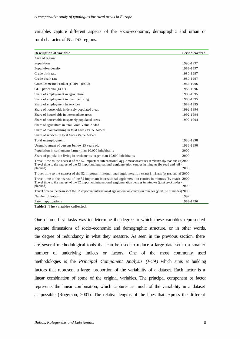
inhabitants. Table 2 lists all the variables that were used. It can be argued that these



variables capture different aspects of the socio-economic, demographic and urban or

rural character of NUTS3 regions.

Description of variable Period covered

Area of region

Population 1995-1997

Population density 1989-1997

Crude birth rate 1980-1997

Crude death rate 1980-1997

Gross Domestic Product (GDP) - (ECU) 1986-1996

GDP per capita (ECU) 1986-1996

Share of employment in agriculture 1988-1995

Share of employment in manufacturing 1988-1995

Share of employment in services 1988-1995

Share of households in densely populated areas 1992-1994

Share of households in intermediate areas 1992-1994

Share of households in sparsely populated areas 1992-1994

Share of agriculture in total Gross Value Added

Share of manufacturing in total Gross Value Added

Share of services in total Gross Value Added

Total unemployment 1988-1998

Unemployment of persons bellow 25 years old 1988-1998

Population in settlements larger than 10.000 inhabitants 2000

Share of population living in settlements larger than 10.000 inhabitants 2000

Travel time to the nearest of the 52 important international agglomeration centres in minutes (by road and air)2000 Travel time to the nearest of the 52 important international agglomeration centres in minutes (by road and rail –planned) 2000

Travel time to the nearest of the 52 important international agglomeration centres in minutes (by road and rail)2000

Travel time to the nearest of the 52 important international agglomeration centres in minutes (by road) 2000 Travel time to the nearest of the 52 important international agglomeration centres in minutes (joint use of modes –planned) 2000

Travel time to the nearest of the 52 important international agglomeration centres in minutes (joint use of modes)2000

Number of hotels 1997

Patent applications 1989-1996

Table 2: The variables collected.

One of our first tasks was to determine the degree to which these variables represented

separate dimensions of socio-economic and demographic structure, or in other words,

the degree of redundancy in what they measure. As seen in the previous section, there

are several methodological tools that can be used to reduce a large data set to a smaller

number of underlying indices or factors. One of the most commonly used

methodologies is the Principal Component Analysis (PCA) which aims at building

factors that represent a large proportion of the variability of a dataset. Each factor is a

linear combination of some of the original variables. The principal component or factor

represents the linear combination, which captures as much of the variability in a dataset

as possible (Rogerson, 2001). The relative lengths of the lines that express the different



variable combinations are called eigenvalues (also known as extraction sums of squared

loadings).

In the context of this study we used PCA to reduce the original variables to a

number of factors that would explain at least 90% of the variance of the original

variables. Figure 1 depicts a plot of all the eigenvalues of all factors. The first

component or factor has an eigenvalue of 31.9 and the graph flattens out at the 21st

component. Further, the 23rd component is the last factor with an eigenvalue above 1.

Scree plot

0

510

1520

25

3035

1 9 17 25 33 41 49 57 65 73 81 89 97 105

113

121

129

137

Component

Eig

enva

lue

Figure 1: Plot of Eigenvalues (Scree Plot)

Table 3 gives details on the first 23 factors.

Total Variance Explained

Initial Eigenvalues Extraction Sums of Squared Loadings Rotation Sums of Squared Loadings Component Total % of

Var. Cumulative % Total % of

Var. Cumulative % Total % of

Var. Cumulative %

1 33.03 22.32 22.32 33.03 22.32 22.32 18.27 12.35 12.35 2 23.84 16.11 38.42 23.84 16.11 38.42 14.30 9.66 22.01 3 13.97 9.44 47.86 13.97 9.44 47.86 13.52 9.13 31.14

4 9.94 6.71 54.58 9.94 6.71 54.58 11.65 7.87 39.01 5 8.30 5.61 60.19 8.30 5.61 60.19 10.81 7.30 46.32

6 5.65 3.82 64.00 5.65 3.82 64.00 9.47 6.40 52.71 7 4.66 3.15 67.15 4.66 3.15 67.15 7.49 5.06 57.77

8 4.24 2.87 70.02 4.24 2.87 70.02 6.54 4.42 62.19 9 3.76 2.54 72.56 3.76 2.54 72.56 5.78 3.90 66.09

10 3.53 2.38 74.94 3.53 2.38 74.94 4.88 3.29 69.38 11 3.00 2.03 76.97 3.00 2.03 76.97 3.79 2.56 71.95

12 2.87 1.94 78.90 2.87 1.94 78.90 3.66 2.48 74.42 13 2.59 1.75 80.65 2.59 1.75 80.65 3.38 2.28 76.70

14 2.23 1.51 82.16 2.23 1.51 82.16 3.21 2.17 78.87 15 2.15 1.46 83.62 2.15 1.46 83.62 2.52 1.71 80.58

16 2.05 1.38 85.00 2.05 1.38 85.00 2.45 1.66 82.23 17 1.96 1.32 86.32 1.96 1.32 86.32 2.36 1.60 83.83 18 1.79 1.21 87.53 1.79 1.21 87.53 2.28 1.54 85.37



19 1.47 0.99 88.52 1.47 0.99 88.52 2.02 1.36 86.73 20 1.27 0.86 89.38 1.27 0.86 89.38 1.93 1.31 88.04 21 1.15 0.78 90.16 1.15 0.78 90.16 1.93 1.30 89.34

22 1.10 0.75 90.90 1.10 0.75 90.90 1.87 1.26 90.61 23 1.05 0.71 91.62 1.05 0.71 91.62 1.49 1.01 91.62

Table 3: Total Variance Explained (Extraction Method: Principal Component Analysis)

As can be seen in table 3, the first 23 factors, which all have an eigenvalue higher than

1, explain 91.62% of the variability of the original variables.

The next step was to perform factor analysis, or in other words, to investigate

the loadings or correlation between the factors and the original variables. To aid in this

investigation the extracted component solutions are rotated in the 149-dimensional

space, so that the loadings tend to be either high or low in absolute value5. In the first

component where unemployment “loaded” highly and it can be argued that this

component describes with a single number what all the unemployment-related variables

represent. Likewise, the second factor has very high loadings of Gross Domestic

Product and Total Average Population. Further, the third factor describes well all the

variables that are related to the Share of Employment in Manufacturing and Services.

Table 4 summarises all factors by the socio-economic or demographic subject that they

best describe. Factors Variables explained 1 Unemployment

2 Total Average Population and GDP 3 Share of employment in services and manufacturing

4 GDP per capita 5 Share of employment in Agriculture

6 Population density 7 Innovation (patent applications)

10 Share of households in densely populated areas 14 Travel time to the nearest of the 52 important international agglomeration centres

12,13,15 Crude birth rate 8,9,21,22 Crude death rate

Table 4: Factor analysis – summary of factors by socio-economic or demographic subject

It can be argued that of particular interest to this project are factors 1,3,4,5,6,7,10 and

14. The next step was to analyse the communalities for all variables. The latter reflect

the degree in which the variables are captured by the first 23 factors6 (which have

eigenvalues above 1). There were over 100 variables that have a communality higher

5 The rotated component matrix and communalities data is available from the authors 6 The communality of each variable is equal to the sum of all squared correlation with each factor



than 0.90. Moreover, the variables that were related to population density in various

years had the highest communalities. In contrast, crude birth rates seemed to have the

highest uniqueness, since they were not highly correlated with the 23 factors.

It is interesting to explore the spatial distribution of the factor scores. Figure 2

depicts the spatial distribution of the unemployment component scores (Factor 1) score

at the NUTS3 level. Areas with negative scores have low unemployment rates, whereas

the areas with high positive factor scores have relatively high unemployment rates. As

can be seen, there are high concentrations of areas with relatively high unemployment

rates in Spain, southern Italy and northern Finland. Moreover, figure 3 shows the

geographical distribution of the Innovation score (Factor 7). As can be seen the regions

with the highest levels of innovation (high positive scores) can be found in central and

northern Europe.

Figure 2: Spatial distribution of factor 1 scores (unemployment)



Figure 3: Spatial distribution of factor 7 scores (innovation)

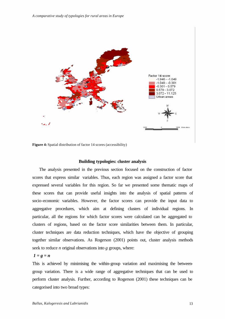
Further, figure 4 represents a thematic map of accessibility based on factor 14, which

describes the variables related to the travel time to the nearest of the 52 important

international agglomeration centres.



Figure 4: Spatial distribution of factor 14 scores (accessibility)

Building typologies: cluster analysis

The analysis presented in the previous section focused on the construction of factor

scores that express similar variables. Thus, each region was assigned a factor score that

expressed several variables for this region. So far we presented some thematic maps of

these scores that can provide useful insights into the analysis of spatial patterns of

socio-economic variables. However, the factor scores can provide the input data to

aggregative procedures, which aim at defining clusters of individual regions. In

particular, all the regions for which factor scores were calculated can be aggregated to

clusters of regions, based on the factor score similarities between them. In particular,

cluster techniques are data reduction techniques, which have the objective of grouping

together similar observations. As Rogerson (2001) points out, cluster analysis methods

seek to reduce n original observations into g groups, where:

1 = g = n

This is achieved by minimising the within-group variation and maximising the between-

group variation. There is a wide range of aggregative techniques that can be used to

perform cluster analysis. Further, according to Rogerson (2001) these techniques can be

categorised into two broad types:



• Agglomerative or hierarchical methods, which start with a number of clusters equal

to the number of observations, which are then merged into larger clusters

• Nonhierarchical or nonagglomerative methods, which begin with an a priori

decision to form g groups and are based on seed points which are equal to the

number of the desired groups (for more details see Rogerson, 2001: pp 199-206).

In the remainder of this section we present how we employed a selection of the above

techniques to classify our regions on the basis of their factor scores.

Hierarchical methods

In this subsection we show the results of an agglomerative approach to cluster analysis,

using the factor scores described above. In particular, we used Ward’s method, which

was developed and presented by Ward (1963) and, according to Rogerson (2001), is one

of the more commonly used hierarchical methods. The method’s aim is to join

observations together into increasing sizes of clusters, using a measure of similarity of

distance. At the start of the Ward’s cluster procedure each observation is in a class by

itself. The next step involves the forming of few but larger clusters on the basis of a

relaxed similarity criterion, until all observations fall within a single cluster in a

hierarchical manner (for more details see Ward, 1963). Figure 5 depicts the results of

the adoption of Ward’s method in the context of our research.



Figure 5: Classification results: Ward’s method

Further, table 5 shows the cluster means of the scores for a selection of factors, which

can facilitate the labelling of the clusters. Cluster/Factor Unemployment Agriculture GDP Population

Density Innovation Accessibility

1 0.088 -0.253 0.176 -0.149 0.081 -0.184

2 -0.603 -0.122 0.376 -0.168 -0.002 -0.142

3 -0.066 -0.239 0.459 -0.397 -0.251 0.123

4 -1.160 1.655 -0.296 -0.162 -0.404 -0.343

5 -0.624 -0.270 0.383 -0.132 -0.190 0.025

6 -0.683 -0.123 0.635 -0.378 -0.223 0.228

7 -0.971 0.619 -0.708 -0.285 -0.433 0.530

8 -1.003 -0.511 1.108 -0.157 -0.069 -0.482

9 -0.544 -0.128 0.313 -0.037 0.135 -0.051

10 0.276 -0.599 -0.085 5.349 0.086 0.123

11 0.335 -0.900 -0.908 0.101 -0.071 -0.254

12 2.112 0.912 -0.206 -0.224 -0.274 -0.306

13 -0.747 2.654 -1.322 0.075 0.558 -0.717

14 -0.152 0.617 -1.006 0.161 -0.135 3.955

15 0.186 1.480 -0.951 0.108 -0.048 -0.022

Table 5: Cluster means of selected factor scores

As can be seen, cluster 12 comprises areas, which have a relatively high mean of the

factor that represents unemployment rates. As can be seen most cluster 12 areas are in

Spain, southern Italy and Ireland. Furthermore, it is noteworthy that areas belonging to



cluster 12 have also relatively low values of the factor that represents innovation. On the

other hand, areas that belong to cluster 4 have relatively low levels of unemployment,

despite the fact that they have an event worst score rating in innovation than cluster 12

areas. Table 6 lists the cluster labels, which were given on the basis of the factor score

cluster means. Cluster Label

1 Service and manufacturing dependent, accessible regions, medium innovation and GDP per capital, relatively low unemployment

2 Agriculture dependent, low unemployment, relatively high GDP per capita

3 Deep rural (low population density), low innovation, relatively inaccessible

4 Low unemployment, low innovation, medium GDP per capita

5 Low unemployment, agriculture dependent

6 Advancing deep rural areas with low population density and low unemployment

7 Intermediate rural areas with low levels of unemployment and medium levels of GDP per capita

8 High GDP per capital rural areas with low levels of unemployment, dependent on Services/manufacturing

9 Accessible rural, low unemployment, relatively high innovation and GDP per capita

10 Relatively high levels of unemployment, low GDP per capita, agriculture dependent, high population density

11 Inaccessible rural areas, low levels of GDP per capita, high unemployment

12 Very high unemployment, low GDP per capita, not dependent on Services and Manufacturing, low innovation

13 Relatively inaccessible rural areas with low unemployment, high innovation levels and low GDP per capita

14 Peripheral inaccessible regions, low levels of innovation and GDP per capita

15 Relatively inaccessible rural areas with low GDP per capita and innovation

Table 6: Cluster labels (Ward’s method)

Using k-means

As noted above, nonhierarchical methods which begin with an a priori decision

to form g groups and are based on seed points which are equal to the number of the

desired groups. In this subsection we show the results of the implementation of such an

approach. In particular, we implemented the k-means procedure with an a-priori

decision to form 15 groups. Figure 6 illustrates the spatial distribution of the derived

clusters, whereas table 7 outlines the cluster means for selected factor scores.



Cluster/Factor Unemployment Agriculture GDP Population Density

Innovation Accessibility

1 -0.624 -0.270 0.383 -0.132 -0.190 0.025

2 -0.552 -0.601 0.743 -0.321 -0.131 -0.001

3 0.048 0.013 -0.438 0.126 -0.127 -0.074

4 -0.392 0.632 5.030 -0.357 4.784 -0.114

5 -0.535 -0.623 0.332 -0.533 -0.120 0.326

6 1.163 0.350 -0.002 -0.327 -0.060 -0.175

7 -1.003 -0.511 1.108 -0.157 -0.069 -0.482

8 -1.160 1.655 -0.296 -0.162 -0.404 -0.343

9 -1.078 1.313 0.309 -0.547 -0.499 0.915

10 -0.971 0.619 -0.708 -0.285 -0.433 0.530

11 -0.030 -0.313 0.634 -0.820 6.808 -0.281

12 0.161 2.542 8.620 13.661 -5.205 -0.228

13 0.177 0.246 -0.142 -0.100 -0.156 4.190

14 0.447 0.275 0.498 9.578 4.758 0.466

15 -0.348 -0.117 0.090 0.000 -0.034 -0.138

Table 7: Cluster means of selected factor scores (k-means)

Figure 6: Classification results: k-means

As can be seen, cluster 6 comprises a relatively large group of regions, which can be

found predominantly in Spain, France and southern Italy, as well as the Republic of

Ireland. These regions have relatively high scores of the Unemployment and Agriculture

factors. Further, cluster 15 is also a large group of regions. In particular, cluster 15

comprises regions with relatively low levels of unemployment and relatively high GDP



per capita. On the other hand, cluster 13 comprises numerous regions, which are

generally inaccessible (high travel times to urban centres).

As it was the case with the clusters that were described in the previous section,

we used the cluster means of the factor scores in the cluster labelling process. Table 8

gives descriptions for all 15 clusters on the basis of their factor score means. Cluster Label

1 Accessible rural regions, low unemployment, relatively high GDP per capita

2 Accessible rural regions, services-based, high GDP per capita , low unemployment

3 Accessible rural with relatively low GDP per capita

4 Advancing rural regions, highly innovative, low unemployment, high GDP, agriculture-based

5 Low unemployment rural regions, services-based, relatively high GDP per capita

6 Very high unemployment regions, agriculture-based, low population density, low innovation.

7 Highly accessible prosperous rural regions with low unemployment, high GDP per capita,

8 Accessible rural regions with low unemployment, agriculture-based

9 Low unemployment, agriculture-based regions, low population density, relatively inaccessible

10 Low unemployment, agriculture-based regions with relatively low GDP per capita, relatively inaccessible

11 Highly innovative advancing regions, accessible, high GDP per capita

12 Agriculture-based advancing peri-urban regions (very high population density)

13 Peripheral inaccessible regions with relatively low levels of unemployment

14 Peri-urban regions with high levels of innovation and GDP per capita

15 Low unemployment regions, not dependent on agriculture, medium levels of innovation and GDP per capita

Table 8: Cluster labels (k-means)

As can be seen, some of the clusters that were produced with the nonhierarchical k-

means method are similar to the hierarchical classification-based clusters described in

the previous section. For instance, the k-means cluster 13 is very similar to cluster 14

described in the previous section (peripheral/inaccessible regions). Likewise, cluster 6 is

similar to cluster 12 of the previous section. Nevertheless, most of the clusters produced

with the two methods differ considerably. It should be noted that there is a wide range

of aggregative clustering methodologies, which would produce alternative results. As

Copus (1996) points out one of the advantages of the methodologies described here is

that they can handle large numbers of variables quickly and are suitable for an

explorative analysis of the data. Further, aggregative approaches to cluster analysis

generate useful and sometimes unexpected information about the patterns in the data.

Moreover, these approaches are considered to be objective and independent of user bias.

However, it can be argued that the use of such methodologies leads to a construction of

a typology, which is highly dependent on the options used when implementing a

particular technique (Copus, 1996). The operator has limited control on the possible

outcome, as this is determined by the statistical relationships between the available

variables. It is possible to experiment with different variable combinations and methods



in order to build a typology, which seems to be in accordance with independent

knowledge and intuition. It is undoubtedly worth exploring other approaches to

classifying rural regions. The following section presents an alternative methodology,

which leads, in our opinion, to a more purposeful and focused classification of

European regions.

Building typologies: a disaggregative approach

So far we have presented a rural classification approach, which was based on

aggregative methodologies, where a number of individual regions has been aggregated

to larger clusters, on the basis of data similarities between them. This section presents

an alternative approach to classifying rural regions according to their rurality and

peripherality. Under this approach, all regions are viewed as a single large group, which

needs to be progressively split into sub-groups, on the basis of a number of pre-selected

discriminatory criteria. In particular, in this section we present a disaggregative

approach, which splits the regions into sub-groups, according to a selection of criteria

that were deemed appropriate for the purposes of this paper.

The disaggregation methodology and selection criteria

The first step in the selection procedure was to exclude all urban areas from the

analysis. In particular, we disaggregated our population of regions into urban and rural

areas. First, we decided to classify as urban all the regions, which had within their

administrative boundaries an urban agglomeration with a population larger than 500,000

inhabitants. Further, we classified as urban all the regions, which had a population of

over 65% living in conurbations with more than 10,000 inhabitants. Based on these

criteria, our initial population of regions was split into rural and urban areas or areas that

had a predominantly urban character. The next step was to further split the rural regions

into sub-groups on the basis of their peripherality.

One of the advantages of the disaggregative approach adopted here, as opposed

to the aggregative cluster analysis presented in the previous section is that the former is

much more flexible than the latter, as it allows the operator or policy analyst to

formulate the classification criteria explicitly and in a transparent and methodologically

simple way (Copus, 1996). However, the main drawback of the disaggregative approach

is the lack of readily available computer software. Thus, in order to implement a

disaggregative methodology we developed a simple program, in the JAVA



programming language7. Further, for the purposes of this project we decided to

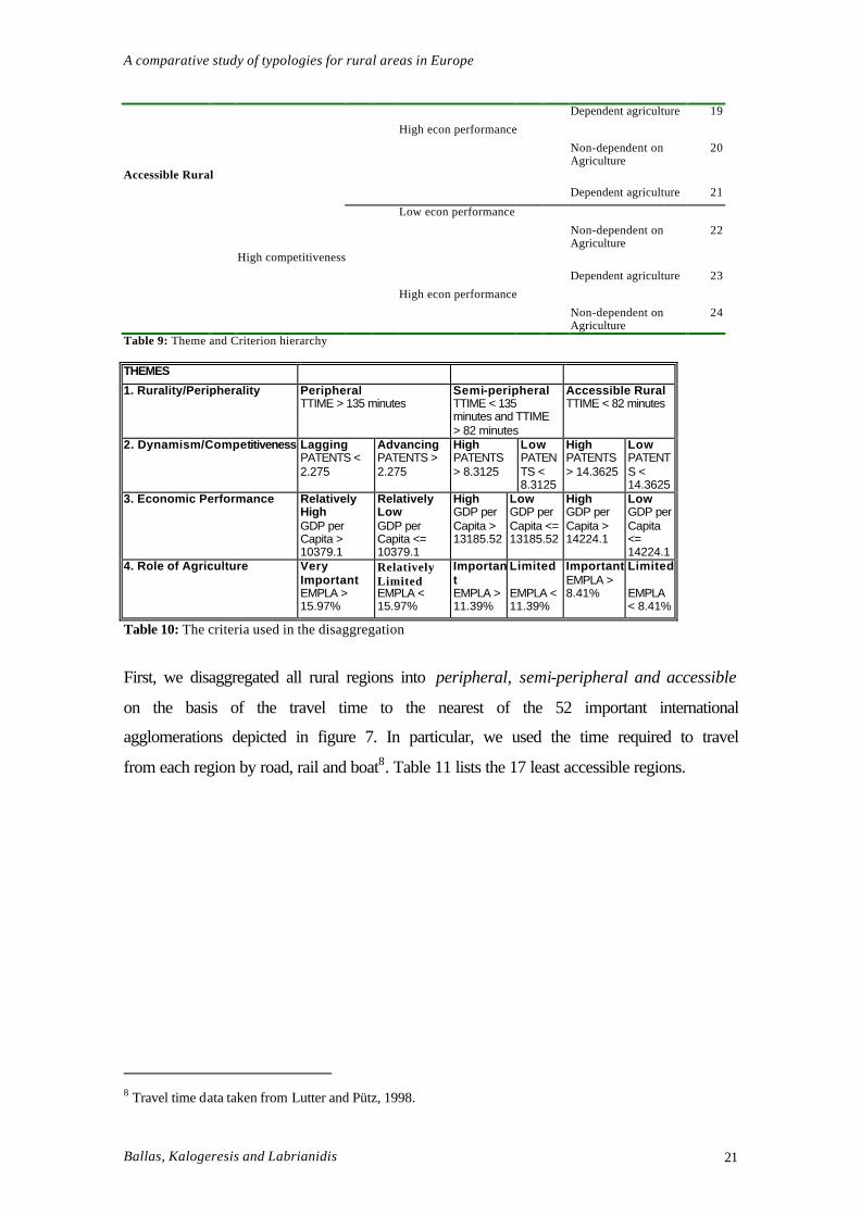
disaggregate all the rural areas into the sub-groups shown in table 9. The selection

criteria used to implement the disaggregation are outlined in table 10. Primary theme Dynamism Economic

Performance Role of Agriculture Types

Dependent on agriculture

1

Low econ performance

Non-dependent on Agriculture

2

Lagging


3

Relatively high econ performance


4

Peripheral

Dependent agriculture 5



6

Advancing


Relatively high econ performance


8


9



10

Low competitiveness


11

High econ performance


12

Semi-peripheral




14

High competitiveness




16




18

Low competitiveness

7 http://java.sun.com/






20

Accessible Rural




22

High competitiveness




24

Table 9: Theme and Criterion hierarchy THEMES

1. Rurality/Peripherality Peripheral TTIME > 135 minutes

Semi-peripheral TTIME < 135 minutes and TTIME > 82 minutes

Accessible Rural TTIME < 82 minutes

2. Dynamism/Competitiveness Lagging PATENTS < 2.275

Advancing PATENTS > 2.275

High PATENTS > 8.3125

Low PATENTS < 8.3125

High PATENTS > 14.3625

Low PATENTS < 14.3625

3. Economic Performance Relatively High GDP per Capita > 10379.1

Relatively Low GDP per Capita <= 10379.1

High GDP per Capita > 13185.52

Low GDP per Capita <= 13185.52

High GDP per Capita > 14224.1

Low GDP per Capita <= 14224.1

4. Role of Agriculture Very Important EMPLA > 15.97%

Relatively Limited EMPLA < 15.97%

Important EMPLA > 11.39%

Limited EMPLA < 11.39%

Important EMPLA > 8.41%

Limited EMPLA < 8.41%

Table 10: The criteria used in the disaggregation

First, we disaggregated all rural regions into peripheral, semi-peripheral and accessible

on the basis of the travel time to the nearest of the 52 important international

agglomerations depicted in figure 7. In particular, we used the time required to travel

from each region by road, rail and boat8. Table 11 lists the 17 least accessible regions.

8 Travel time data taken from Lutter and Pütz, 1998.



Region Travel time in

minutes GR421 Dodekanisos 1267

GR411 Lesvos 744

GR432 Lasithi 738

GR433 Rethymno 699

GR431 Irakleio 697

GR434 Chania 667

ITB04 Cagliari 665

GR412 Samos 639

ITB03 Oristano 603

GR413 Chios 594

SE082 Norrbottens län 584

ITB01 Sassari 553

ITB02 Nuoro 548

FI152 Lappi 539

SE081 Västerbottens län 508

UKM46 Shetland Islands 501

Table 11: Travel time by rail, road and boat to the nearest of the 52 agglomeration centres depicted in figure 8

After exploring various combinations of travel time-based criteria we concluded that it

would be reasonable to define as peripheral the 25% of regions with the highest travel

time (211 regions in total). ? ll these rural regions had a travel time, which was more

than 135 minutes.

Likewise, we defined as accessible rural the 50% of regions with the lowest

travel time and as semi-peripheral all the remaining regions. As can be seen in table 10

all the semi-peripheral regions had a travel time less than 135 minutes and more than 82

minutes, whereas the accessible rural areas had travel times less than 82 minutes.

Figure 8 depicts the spatial distribution of all the regions.



Figure 7: 52 important international agglomeration centres



Figure 8: Spatial distribution of European regions after the first disaggregation

The next step in the analysis was to further disaggregate the regions on the basis of their

economic dynamism and competitiveness. It can be argued that the latter is expressed to

a certain degree by the number of patent applications in each region. Moreover, it can

be argued that regional innovation expressed through the numbers of patent applications

is of particular interest, in the light of the increasing significance of industrial creativity

to regional economic progress. In the context of this paper we used the average number

of patent applications in each region for the years 1989-96 as a competitiveness and

economic dynamism criterion. Nevertheless, it should be noted that the values of the

thresholds were determined on the basis of the type of area being disaggregated. For

instance, as can be seen in table 10, all peripheral areas were split into advancing and

lagging using the 2.275 threshold, which is the median of this variable for all peripheral

areas. Likewise, the patent application thresholds that were used to determine the

dynamism and competitiveness of semi-peripheral and accessible rural areas were

8.3125 and 14.3625 respectively. The reason for adopting this approach to determining

disaggregation thresholds is that the use of the same threshold for different types of

areas can lead to meaningless classifications (e.g. using the patents threshold of 8.3125



to split peripheral areas into advancing and lagging would mean that all peripheral

areas would be classified as lagging, as there may be no peripheral areas with such a

high number of patent applications). As a result of the second disaggregation, the 211

peripheral regions were split into lagging (105 regions) and advancing (106 regions). In

addition, the semi-peripheral and accessible rural regions were disaggregated into areas

of high and low competitiveness (419 and 420 regions respectively). In a similar

manner, all semi-peripheral regions were further disaggregated into areas of high and

low economic performance and subsequently into agriculture-dependent regions and

regions where the role of agriculture is not so important. Table 10 gives more details on

the criteria and thresholds that were used. The final result of all 4 disaggregations was

the typology shown in table 12. Moreover, figure 9 depicts the spatial distribution of all

regions by type.

Disaggregative typology number of regions

% of total EU NUTS3 regions

1. Peripheral, lagging, relatively low economic performance, dependent on agriculture 37 3.30%

2 Peripheral, lagging, relatively low economic performance, not dependent on agriculture 52 4.70%

3. Peripheral, advancing, relatively low economic performance, dependent on agriculture 3 0.30%

4. Peripheral, advancing, relatively low economic performance, not dependent on agriculture 13 1.20%

5. Peripheral, lagging, relatively high economic performance, dependent on agriculture 4 0.40%

6. Peripheral, lagging, relatively high economic performance, non-dependent on agriculture 12 1.10%

7. Peripheral, advancing, relatively high economic performance, dependent on agriculture 10 0.90%

8. Peripheral, advancing, relatively high economic performance, non-dependent on agriculture 80 7.20%

9. Semi-peripheral , low competitiveness, low economic performance, dependent on agriculture 28 2.50%

10. Semi-peripheral , low competitiveness, low economic performance, not dependent on agriculture 48 4.30%

11. Semi-peripheral , high competitiveness, low economic performance, dependent on agriculture 10 0.90%

12. Semi-peripheral , high competitiveness, low economic performance, not dependent on agriculture 18 1.60%

13. Semi-peripheral , low competitiveness, high economic performance, dependent on agriculture 5 0.50%

14. Semi-peripheral , low competitiveness, high economic performance, non-dependent on agriculture 23 2.10%

15. Semi-peripheral , high competitiveness, high economic performance, dependent on agriculture 9 0.80%

16. Semi-peripheral , high competitiveness, high economic performance, non-dependent on agriculture 68 6.10%

17. Accessible rural, low competitiveness, low economic performance, dependent on agriculture 54 4.90%

18. Accessible rural, low competitiveness, low economic performance, non-dependent on agriculture 95 8.60%

19. Accessible rural, high competitiveness, low economic performance, dependent on agriculture 11 1.00%

20. Accessible rural, high competitiveness, low economic performance, non-dependent on agriculture 49 4.40%

21. Accessible rural, low competitiveness, high economic performance, dependent on agriculture 21 1.90%

22. Accessible rural, low competitiveness, high economic performance, non-dependent on agriculture 39 3.50%

23. Accessible rural, high competitiveness, high economic performance, dependent on agriculture 20 1.80%

24. Accessible rural, high competitiveness, high economic performance, non-dependent on agriculture 130 11.70%

25. Urban areas 268 24.20%

Table 12: The disaggregative types



20 0 0 200 400 600 800 Kilometers

all r egi ons12345678910111213141516171819202122232425

Figure 9: Final typology results

It can be argued that the use of patent application as a variable is one of the most

innovative features of this research. Regional innovation is becoming increasingly

important, as economies become more complex and a greater variety of goods and ideas

are patented (Ceh, 2001). The remainder of this section discusses the patterns in the

geographical distribution of different types of regions.

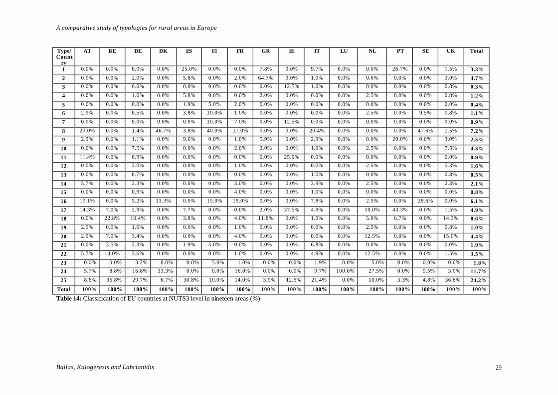
There are 1,107 NUTS3 areas in EU. More than 70% of NUTS3 areas are in

four countries (Germany, UK, Italy and France – see table 13). In fact the most

important type is 25 (i.e. urban areas), which constitutes 24.2% of all NUTS3 areas in

EU. More precisely “Urban areas” constitute a very significant proportion of NUTS3

areas in Belgium, UK, Spain and Germany (table 14).

If we exclude urban areas the rest of the NUTS3 regions are divided in three

groups. Five countries have more than 50% of their regions classified in the peripheral



regions (types 1-8). That is, 77.5% of Greece’s NUTS3 regions are peripheral, 72.3% of

Finland’s, 66.7% of Spain’s, 60% of Sweden’s and 50% of Denmark’s.

On the other extreme five countries have more than 50% of their regions

classified in the accessible rural regions category (types 17 to 24). That is, 100% of

Luxemburg’s and Belgium’s NUTS3 regions are accessible rural, 83.5% of

Netherlands’s, 62.9% of Germany’s, and 57.2% of UK’s (table 15). The next sections

discuss the spatial distribution of each region type in more detail.

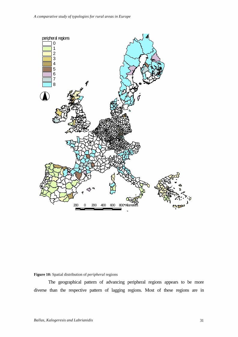
The peripheral regions

There are 211 regions classified as peripheral (types 1-8), of which 105 and 106

are further classified as lagging and advancing respectively (see figure 10). Most

peripheral lagging regions are concentrated in Southern Europe, and in particular,

Portugal, western Spain, southern Italy and eastern and western Greece and most of the

Greek Islands. Nevertheless, it is noteworthy that there are several peripheral lagging

regions in the Scandinavian countries. Further, there are some peripheral-lagging

regions in Germany and the United Kingdom (mostly in Scotland, Wales and Cornwall)

too.



Type/Country AT BE DE DK ES FI FR GR IE IT LU NL PT SE UK Total Total

(%) 1 0 0 0 0 13 0 0 4 0 10 0 0 8 0 2 37 3.3% 2 0 0 9 0 3 0 2 33 0 1 0 0 0 0 4 52 4.7% 3 0 0 0 0 0 0 0 0 1 1 0 0 0 0 1 3 0.3% 4 0 0 7 0 3 0 0 1 0 0 0 1 0 0 1 13 1.2% 5 0 0 0 0 1 1 2 0 0 0 0 0 0 0 0 4 0.4% 6 1 0 2 0 2 2 1 0 0 0 0 1 0 2 1 12 1.1% 7 0 0 0 0 0 2 7 0 1 0 0 0 0 0 0 10 0.9% 8 7 0 6 7 2 8 17 0 0 21 0 0 0 10 2 80 7.2% 9 1 0 5 0 5 0 1 3 0 3 0 0 6 0 4 28 2.5%

10 0 0 33 0 0 0 2 1 0 1 0 1 0 0 10 48 4.3% 11 4 0 4 0 0 0 0 0 2 0 0 0 0 0 0 10 0.9% 12 0 0 9 0 0 0 1 0 0 0 0 1 0 0 7 18 1.6% 13 0 0 3 0 0 0 0 0 0 1 0 0 0 0 1 5 0.5% 14 2 0 10 0 0 0 3 0 0 4 0 1 0 0 3 23 2.1% 15 0 0 4 0 0 0 4 0 0 1 0 0 0 0 0 9 0.8% 16 6 0 23 2 0 3 19 0 0 8 0 1 0 6 0 68 6.1% 17 5 4 13 0 4 0 0 1 3 5 0 4 13 0 2 54 4.9% 18 0 13 46 0 2 0 4 6 0 1 0 2 2 0 19 95 8.6% 19 1 0 7 0 0 0 1 0 0 0 0 1 0 0 1 11 1.0% 20 1 4 15 0 0 0 4 0 0 0 0 5 0 0 20 49 4.4% 21 0 2 10 0 1 1 0 0 0 7 0 0 0 0 0 21 1.9% 22 2 8 16 0 0 0 1 0 0 5 0 5 0 0 2 39 3.5% 23 0 0 14 0 0 1 1 0 0 2 0 2 0 0 0 20 1.8% 24 2 5 74 5 0 0 16 0 0 10 1 11 0 2 4 130 11.7% 25 3 21 131 1 16 2 14 2 1 22 0 4 1 1 49 268 24.2%

Total 35 57 441 15 52 20 100 51 8 103 1 40 30 21 133 1107 3.3%

Total (%) 3.2% 5.1% 39.8% 1.4% 4.7% 1.8% 9.0% 4.6% 0.7% 9.3% 0.1% 3.6% 2.7% 1.9% 12.0% à

100% Table 13: Classification of EU countries at NUTS3 level in nineteen areas (a.n.)



Type/Count

ry

AT BE DE DK ES FI FR GR IE IT LU NL PT SE UK Total

1 0.0% 0.0% 0.0% 0.0% 25.0% 0.0% 0.0% 7.8% 0.0% 9.7% 0.0% 0.0% 26.7% 0.0% 1.5% 3.3%

2 0.0% 0.0% 2.0% 0.0% 5.8% 0.0% 2.0% 64.7% 0.0% 1.0% 0.0% 0.0% 0.0% 0.0% 3.0% 4.7%

3 0.0% 0.0% 0.0% 0.0% 0.0% 0.0% 0.0% 0.0% 12.5% 1.0% 0.0% 0.0% 0.0% 0.0% 0.8% 0.3%

4 0.0% 0.0% 1.6% 0.0% 5.8% 0.0% 0.0% 2.0% 0.0% 0.0% 0.0% 2.5% 0.0% 0.0% 0.8% 1.2%

5 0.0% 0.0% 0.0% 0.0% 1.9% 5.0% 2.0% 0.0% 0.0% 0.0% 0.0% 0.0% 0.0% 0.0% 0.0% 0.4%

6 2.9% 0.0% 0.5% 0.0% 3.8% 10.0% 1.0% 0.0% 0.0% 0.0% 0.0% 2.5% 0.0% 9.5% 0.8% 1.1%

7 0.0% 0.0% 0.0% 0.0% 0.0% 10.0% 7.0% 0.0% 12.5% 0.0% 0.0% 0.0% 0.0% 0.0% 0.0% 0.9%

8 20.0% 0.0% 1.4% 46.7% 3.8% 40.0% 17.0% 0.0% 0.0% 20.4% 0.0% 0.0% 0.0% 47.6% 1.5% 7.2%

9 2.9% 0.0% 1.1% 0.0% 9.6% 0.0% 1.0% 5.9% 0.0% 2.9% 0.0% 0.0% 20.0% 0.0% 3.0% 2.5%

10 0.0% 0.0% 7.5% 0.0% 0.0% 0.0% 2.0% 2.0% 0.0% 1.0% 0.0% 2.5% 0.0% 0.0% 7.5% 4.3%

11 11.4% 0.0% 0.9% 0.0% 0.0% 0.0% 0.0% 0.0% 25.0% 0.0% 0.0% 0.0% 0.0% 0.0% 0.0% 0.9%

12 0.0% 0.0% 2.0% 0.0% 0.0% 0.0% 1.0% 0.0% 0.0% 0.0% 0.0% 2.5% 0.0% 0.0% 5.3% 1.6%

13 0.0% 0.0% 0.7% 0.0% 0.0% 0.0% 0.0% 0.0% 0.0% 1.0% 0.0% 0.0% 0.0% 0.0% 0.8% 0.5%

14 5.7% 0.0% 2.3% 0.0% 0.0% 0.0% 3.0% 0.0% 0.0% 3.9% 0.0% 2.5% 0.0% 0.0% 2.3% 2.1%

15 0.0% 0.0% 0.9% 0.0% 0.0% 0.0% 4.0% 0.0% 0.0% 1.0% 0.0% 0.0% 0.0% 0.0% 0.0% 0.8%

16 17.1% 0.0% 5.2% 13.3% 0.0% 15.0% 19.0% 0.0% 0.0% 7.8% 0.0% 2.5% 0.0% 28.6% 0.0% 6.1%

17 14.3% 7.0% 2.9% 0.0% 7.7% 0.0% 0.0% 2.0% 37.5% 4.9% 0.0% 10.0% 43.3% 0.0% 1.5% 4.9%

18 0.0% 22.8% 10.4% 0.0% 3.8% 0.0% 4.0% 11.8% 0.0% 1.0% 0.0% 5.0% 6.7% 0.0% 14.3% 8.6%

19 2.9% 0.0% 1.6% 0.0% 0.0% 0.0% 1.0% 0.0% 0.0% 0.0% 0.0% 2.5% 0.0% 0.0% 0.8% 1.0%

20 2.9% 7.0% 3.4% 0.0% 0.0% 0.0% 4.0% 0.0% 0.0% 0.0% 0.0% 12.5% 0.0% 0.0% 15.0% 4.4%

21 0.0% 3.5% 2.3% 0.0% 1.9% 5.0% 0.0% 0.0% 0.0% 6.8% 0.0% 0.0% 0.0% 0.0% 0.0% 1.9%

22 5.7% 14.0% 3.6% 0.0% 0.0% 0.0% 1.0% 0.0% 0.0% 4.9% 0.0% 12.5% 0.0% 0.0% 1.5% 3.5%

23 0.0% 0.0% 3.2% 0.0% 0.0% 5.0% 1.0% 0.0% 0.0% 1.9% 0.0% 5.0% 0.0% 0.0% 0.0% 1.8%

24 5.7% 8.8% 16.8% 33.3% 0.0% 0.0% 16.0% 0.0% 0.0% 9.7% 100.0% 27.5% 0.0% 9.5% 3.0% 11.7%

25 8.6% 36.8% 29.7% 6.7% 30.8% 10.0% 14.0% 3.9% 12.5% 21.4% 0.0% 10.0% 3.3% 4.8% 36.8% 24.2%

Total 100% 100% 100% 100% 100% 100% 100% 100% 100% 100% 100% 100% 100% 100% 100% 100%

Table 14: Classification of EU countries at NUTS3 level in nineteen areas (%)



Type/Country AT BE DE DK ES FI FR GR IE IT LU NL PT SE UK Total

1 0.0% 0.0% 0.0% 0.0% 36.1% 0.0% 0.0% 8.2% 0.0% 12.3% 0.0% 0.0% 27.6% 0.0% 2.4% 4.4%

2 0.0% 0.0% 2.9% 0.0% 8.3% 0.0% 2.3% 67.3% 0.0% 1.2% 0.0% 0.0% 0.0% 0.0% 4.8% 6.2%

3 0.0% 0.0% 0.0% 0.0% 0.0% 0.0% 0.0% 0.0% 14.3% 1.2% 0.0% 0.0% 0.0% 0.0% 1.2% 0.4%

4 0.0% 0.0% 2.3% 0.0% 8.3% 0.0% 0.0% 2.0% 0.0% 0.0% 0.0% 2.8% 0.0% 0.0% 1.2% 1.5%

5 0.0% 0.0% 0.0% 0.0% 2.8% 5.6% 2.3% 0.0% 0.0% 0.0% 0.0% 0.0% 0.0% 0.0% 0.0% 0.5%

6 3.1% 0.0% 0.6% 0.0% 5.6% 11.1% 1.2% 0.0% 0.0% 0.0% 0.0% 2.8% 0.0% 10.0% 1.2% 1.4%

7 0.0% 0.0% 0.0% 0.0% 0.0% 11.1% 8.1% 0.0% 14.3% 0.0% 0.0% 0.0% 0.0% 0.0% 0.0% 1.2%

8 21.9% 0.0% 1.9% 50.0% 5.6% 44.4% 19.8% 0.0% 0.0% 25.9% 0.0% 0.0% 0.0% 50.0% 2.4% 9.5%

9 3.1% 0.0% 1.6% 0.0% 13.9% 0.0% 1.2% 6.1% 0.0% 3.7% 0.0% 0.0% 20.7% 0.0% 4.8% 3.3%

10 0.0% 0.0% 10.6% 0.0% 0.0% 0.0% 2.3% 2.0% 0.0% 1.2% 0.0% 2.8% 0.0% 0.0% 11.9% 5.7%

11 12.5% 0.0% 1.3% 0.0% 0.0% 0.0% 0.0% 0.0% 28.6% 0.0% 0.0% 0.0% 0.0% 0.0% 0.0% 1.2%

12 0.0% 0.0% 2.9% 0.0% 0.0% 0.0% 1.2% 0.0% 0.0% 0.0% 0.0% 2.8% 0.0% 0.0% 8.3% 2.1%

13 0.0% 0.0% 1.0% 0.0% 0.0% 0.0% 0.0% 0.0% 0.0% 1.2% 0.0% 0.0% 0.0% 0.0% 1.2% 0.6%

14 6.3% 0.0% 3.2% 0.0% 0.0% 0.0% 3.5% 0.0% 0.0% 4.9% 0.0% 2.8% 0.0% 0.0% 3.6% 2.7%

15 0.0% 0.0% 1.3% 0.0% 0.0% 0.0% 4.7% 0.0% 0.0% 1.2% 0.0% 0.0% 0.0% 0.0% 0.0% 1.1%

16 18.8% 0.0% 7.4% 14.3% 0.0% 16.7% 22.1% 0.0% 0.0% 9.9% 0.0% 2.8% 0.0% 30.0% 0.0% 8.1%

17 15.6% 11.1% 4.2% 0.0% 11.1% 0.0% 0.0% 2.0% 42.9% 6.2% 0.0% 11.1% 44.8% 0.0% 2.4% 6.4%

18 0.0% 36.1% 14.8% 0.0% 5.6% 0.0% 4.7% 12.2% 0.0% 1.2% 0.0% 5.6% 6.9% 0.0% 22.6% 11.3%

19 3.1% 0.0% 2.3% 0.0% 0.0% 0.0% 1.2% 0.0% 0.0% 0.0% 0.0% 2.8% 0.0% 0.0% 1.2% 1.3%

20 3.1% 11.1% 4.8% 0.0% 0.0% 0.0% 4.7% 0.0% 0.0% 0.0% 0.0% 13.9% 0.0% 0.0% 23.8% 5.8%

21 0.0% 5.6% 3.2% 0.0% 2.8% 5.6% 0.0% 0.0% 0.0% 8.6% 0.0% 0.0% 0.0% 0.0% 0.0% 2.5%

22 6.3% 22.2% 5.2% 0.0% 0.0% 0.0% 1.2% 0.0% 0.0% 6.2% 0.0% 13.9% 0.0% 0.0% 2.4% 4.6%

23 0.0% 0.0% 4.5% 0.0% 0.0% 5.6% 1.2% 0.0% 0.0% 2.5% 0.0% 5.6% 0.0% 0.0% 0.0% 2.4%

24 6.3% 13.9% 23.9% 35.7% 0.0% 0.0% 18.6% 0.0% 0.0% 12.3% 100.0% 30.6% 0.0% 10.0% 4.8% 15.5%

Total 100% 100% 100% 100% 100% 100% 100% 100% 100% 100% 100% 100% 100% 100% 100% 100%

Table 15: Classification of EU countries at NUTS3 level in eighteen different non urban areas (%)



200 0 200 400 600 800 Kilometers

peripheral regions012345678

Figure 10: Spatial distribution of peripheral regions

The geographical pattern of advancing peripheral regions appears to be more

diverse than the respective pattern of lagging regions. Most of these regions are in



central and northern Italy, northern Spain, central and western France, Eastern Germany

and Austria, most of the northern parts of Denmark and Sweden and western Ireland.

All of the Portuguese, most of the Spanish and many of the French peripheral

regions are dependent on agriculture. Surprisingly, this does not appear to be the case in

Greece, where only a minority of regions in the southern mainland is dependent on

agriculture. Naturally, the situation is significantly more straightforward when it comes

to economic performance, where there is a quite visible divide between the traditional

European periphery (Greece, Portugal, Spain, S. Italy and Ireland) and the other parts of

Europe, with the former (except some parts of Spain and Ireland) characterised by low

economic performance. The only other cases of low economic performance are found in

some of the former East German NUTS3 peripheral rural regions, and quite

unexpectedly, in most British peripheral regions.

The semi-peripheral regions

There are 209 regions that are classified as Semi-peripheral (types 9-16- see

figure 11) and they are mainly in Germany, France, Italy, the Netherlands and the UK

less in Finland, Sweden, Greece, Spain and Portugal.

There is significant variation in the distribution of particular types of Semi-

peripheral regions. Precisely, the Semi-peripheral regions which have low

competitiveness, low economic performance and are dependent on agriculture (type 9

regions) are mainly in western Spain and Portugal, southern Italy, central Greece,

Northern Ireland and eastern Germany. In contrast, the most affluent areas, which are

highly competitive and attain high levels of economic performance (type 16), are mostly

in northern Europe. Most of them are found in France, northern Italy, Germany, Sweden

and Finland. It is noteworthy that France and Italy are the only member states, which

have regions that belong to different subtypes of Semi-peripheral regions. It can thus be

argued that there is a greater degree of dualism and polarisation in these countries. In

contrast, the rest of the Mediterranean member states have predominantly Semi-

peripheral regions of low competitiveness and economic performance. On the other

hand, the northern member states have predominantly highly competitive and affluent

regions. This trend becomes more apparent in the next section, which discusses the

geographical patterns in the distribution of accessible rural regions.



200 0 200 400 600 800 Kilometers

semi-peripheral regionsnon semi-peripheral910111213141516

Figure 11: Spatial distribution of semi-peripheral regions

The accessible rural regions

Most of the 419 accessible rural regions are found in central, northern and

north-west Europe (see figure 12). It is noteworthy that more than half of these regions



are concentrated in Germany. Six countries have more than 50% of their non-urban

areas classified in this category (types 17 to 24). That is, 100% of Luxemburg’s and

Belgium’s, 83.5% of Netherlands’s, 62.9% of Germany’s, 57.2% of UK’s and 51.7% of

Portugal’s, NUTS3 regions are accessible rural.

200 0 200 400 600 800 Kilometers

accessible regionsnon-accessible1718192021222324

Figure 12: Spatial distribution of accessible regions.



What is interesting is that Portugal’s accessible rural regions are almost

exclusively concentrated in type 17 (low competitiveness – low economic performance

- dependent on agriculture) and to a lesser extent in type 18 (low competitiveness – low

economic performance - non-dependent on agriculture).

Conclusions

As can be seen, the countries that have the majority of their regions to be least

competitive are: Greece, Spain, Portugal, Ireland and Italy. In most of these regions

agriculture plays a relatively important role. It should be noted though that there are also

several least competitive regions with low economic performance in the United

Kingdom, Eastern Germany and Austria. However, in most of these regions the role of

agriculture is much less significant than in their southern European counterparts and

Ireland.

On the other hand, the countries that have a majority of highly competitive

regions with high levels of economic performance can be found in central Europe

(predominantly in Germany and north-west France) and Northern Europe (The

Netherlands and Denmark). Further, there are some regions of this type in the

Scandinavian member states and in the United Kingdom. It is also noteworthy that the

latter has a high number of regions that are highly competitive but attain relatively low

levels of economic performance.

Overall, the outcome of the methodology adopted was quite satisfactory. Unlike

most other classifications, it manages to depict quite well the various national

differences. This is particularly important in the case of the smaller countries, such as

Greece or Portugal, which, in most other classifications, usually fall into two or three

classes. There are however, shortcomings to the approach. The most significant one is

the fact that the outcome depends heavily on the choice of themes. Hence, it is quite

clear that the results would be different had we used a different sequence of themes. In

other words, this is by no means a universal classification of European regions. Nor do

we think that such a classification is feasible, although it would undoubtedly be useful.

The reason is that secondary data is not capable of depicting the various processes at

work, or the historical trajectories of each region.

In this context, classifications (including ours) should only be used as mere

approximations of very complex and contextual realities and as guidelines into more

thorough analysis.



Acknowledgements: The authors acknowledge support from an FP5 grant for the

project “The Future of Europe’s Rural Periphery: The Role of Entrepreneurship in

Responding to Employment Problems and Social Marginalisation” (HPSE-CT-00013).

The authors would like to thank Seraphim Alvanides (University of Newcastle, UK) for

his comments on an earlier draft of this paper.

References

Batey P.W.J., Brown P.J. 1995, From human ecology to customer targeting: the

evolution of geodemographics, in P.Longley & G.P.Clarke (eds) GIS for business

and service planning, Geoinformation, Cambridge, 77-103

Batey, P., Brown, P., and Corver, M. 1999. Participation in higher education: a

geodemographic perspective on the potential for further expansion in student

numbers, Journal of Geographical Systems, vol. 1, pp. 277-303

Birkin, M, Customer Targeting, Geodemographics and Lifestyle Approaches, in

P.Longley & G.P.Clarke (eds) GIS for business and service planning,

Geoinformation, Cambridge

Blunden, J. R., Pryce, W. T. R. and Dreyer, P. 1998. The classification of Rural Areas

in the European Context: An Exploration of a Typology Using Neural Network

Applications, Regional Studies vol. 32, pp.149-160

Brunsdon, C. 1995, Further analysis of multivariate census data, in Openshaw, S.

(ed.), Census Users’ Handbook, GeoInformation International, London, pp. 271-

306

Ceh, B. (2001), Regional innovation potential in the United States: Evidence of

spatial transformation, Papers in Regional Science vol. 80, pp.297-316

Cloke J.P. 1977. An index of rurality in England and Wales. Regional Studies vol 11,

pp. 31-46.

Cloke J.P. and Edwards G.1986 Rurality in England and Wales 1981. Regional Studies

vol 20(4), pp. 289-306.

Copus, A (1996), A Rural Development Typology of European NUTS III Regions,

Working Paper 14, Agricultural and Rural Economics Department, Scotish

Agricultural College, Aberdeen

Errington A J. (1990) Rural employment in England: some data sources and their use,

Journal of Agricultural Economics 41, 47 - 61.

EU Commission 1988. The future of rural society. COM (88) 501. Brussels (WP 14)



EU Commission 1992. Final report from TYPORA. A study on the typology of rural

areas for telematics applications. Luxemburg. (WP 14)

Ibery B. 1981. Dorset agriculture. A classification of regional types. Transactions of the

Institute of British geographers 6, pp. 214-227 (WP 14)

Kostowicki 1989. “Types of agriculture in Britain in the light of types of agriculture

map of Europe”, Geographia Polonica 56, pp. 133-154. (WP 14)

Labrianidis L., Ferrao J., Hertzina K., Kalantaridis C., Piasecki B., Smallbone D.

2003.The future of Europe’s rural periphery. Final Report. 5th Framework

Programme of the European Community

Leavy, A., McDonagh, P. and Commins, P. 1999. Public Policy Trends and Some

Regional Impacts, Rural Economy Research Series no. 6, Agricultural and Food

Development Authority (Teagasc), Dublin.

Longley P.A. and Clarke, G (1995) (eds), GIS for business and service planning,

Geoinformation, Cambridge

Lutter H. and Pütz T. (1998) Strategie für einen raum- und

umweltverträglichen Personenfernver-kehr, in: Informationen zur

Raumentwicklung Heft 6.1998 (in German)

Malinen P. Keranen R. and Keranen H, 1994. Rural area typology in Finland. Oulu

(WP 14)

OECD 1994 Creating rural indicators. OECD.

OECD 1996 Rural employment indicators. OECD.

Openshaw, S. 1983. Multivariate analysis of census data: the classification of areas. A

Census Users' Handbook. D. Rhind(ed.). London, Methuen, pp. 243-264.

Openshaw, S. 1983. Rural area classification using census data, Geographia

Polonica, vol. 51, 285-99

Pettersson, Ö. 2001. Microregional fragmentation in a Swedish county, Papers in

Regional Science, vol. 80, pp. 389-409.

Reading, R. Openshaw, S. and Jarvis, S. 1994. Are multidimensional Social

Classifications of Areas Useful in UK Health-Service Research. Journal of

Epidemiology and Community Health 48(2): 192-200.

Rees, P. Denham, C. Charlton, J. Openshaw, S. Blake, M. and See, L. 2002. ONS

Classifications and GB Profiles: Census Typologies for Researchers, in P. Rees,

Martin, D., & Williamson, P. (eds) The Census Data System, Chichester, Wiley.

Rogerson, P. A., 2001, Statistical Methods for Geography, Sage, London



Shucksmith M. 1990. The definition of rural areas and rural deprivation, Scottish Homes

Research Report 2 (WP 21 Esparcia + Tur)

Ward, J. H. (1963). Hierarchical grouping to optimize an objective function. Journal of

the American Statistical Association 58(30): 236-244

cen tre for computational geography, school of geography

Documents