THE UNIVERSITY of EDINBURGH

Project in Mathematics (Group)

Celtic Knot Theory

Authors:

Jessica Connor

Nick Ward

Supervisors:

Andrew Ranicki

Julia Collins

March 12, 2012

Abstract

The purpose of this project is to explore the subject of knot theory. We consider

knot invariants, in particular the Alexander polynomial which we show to be well

defined and invariant and also the Alexander-Conway polynomial. We discuss

both alternating and non-alternating knots in relation to such invariants. The

main part of the paper concerns Celtic knots; their construction and the proofs

that Celtic knots are alternating, and that alternating knots are Celtic. Finally

we investigate another example of mathematical knots in art, the Brunnian links.

Summary

This project report is submitted in partial fulfilment of the requirements for the

degree of BSc Mathematics.

2

Contents

Abstract 2

1 Introduction 5

2 Knot Theory 7

2.1 History of Knots . . . . . . . . . . . . . . . . . . . . . . . . . . . 7

2.2 Knots in Context . . . . . . . . . . . . . . . . . . . . . . . . . . . 9

3 Polynomial Invariants 12

3.1 The Alexander Polynomial . . . . . . . . . . . . . . . . . . . . . . 12

3.1.1 Proof that ∆K(t) is well defined . . . . . . . . . . . . . . . 13

3.1.2 Proof of Invariance . . . . . . . . . . . . . . . . . . . . . . 17

3.2 The Alexander-Conway Polynomial . . . . . . . . . . . . . . . . . 21

3.2.1 Calculation for Figure Eight Knot . . . . . . . . . . . . . . 23

3.3 Further Polynomial Invariants . . . . . . . . . . . . . . . . . . . . 23

4 Alternating Knots 25

4.1 Examples . . . . . . . . . . . . . . . . . . . . . . . . . . . . . . . 25

4.1.1 Trefoil Knot, 31 . . . . . . . . . . . . . . . . . . . . . . . . 25

4.1.2 Figure Eight Knot, 41 . . . . . . . . . . . . . . . . . . . . 26

4.2 Properties . . . . . . . . . . . . . . . . . . . . . . . . . . . . . . . 27

5 Non-alternating Knots 29

6 Celtic Knots 31

6.1 What is a Celtic knot? . . . . . . . . . . . . . . . . . . . . . . . . 31

6.2 Construction . . . . . . . . . . . . . . . . . . . . . . . . . . . . . 33

3

CONTENTS

6.3 Celtic Knots vs. Alternating Knots . . . . . . . . . . . . . . . . . 34

6.3.1 Celtic Knots . . . . . . . . . . . . . . . . . . . . . . . . . . 34

6.3.2 Alternating Knots . . . . . . . . . . . . . . . . . . . . . . . 35

6.4 Polynomials of Celtic Knots . . . . . . . . . . . . . . . . . . . . . 42

6.5 Celtic Invariants . . . . . . . . . . . . . . . . . . . . . . . . . . . . 45

7 Brunnian Links 47

7.1 n = 3: Borromean Rings, 632 . . . . . . . . . . . . . . . . . . . . . 48

7.2 Celtic Borromean Rings . . . . . . . . . . . . . . . . . . . . . . . 48

8 Conclusion 50

Glossary 51

4

Chapter 1

Introduction

In this paper we give an introduction to knot theory, the study of mathematical

knots. While inspired by knots that we see in real life, in ropes, laces and wires,

a mathematical knot differs in that the two loose ends of a strand are joined to-

gether. This forms a continuous loop which cannot be undone by manipulation.

In mathematical terminology we say that a knot1 is an embedding of S1 (a circle)

in R3 that does not intersect itself.

Knot theory may seem to stand alone as a field of study, but it has strong

connections to many other mathematical fields, in particular topology and graph

theory. Outside of mathematics, the study of knots has major applications in

other disciplines such as physics, biology and chemistry. We discuss how knot

theory has developed historically and the implications it has had to date. We also

show that it is a very current area of study with many problems left unsolved.

The great unsolved problem in knot theory is how to tell when two knots

are equivalent by using knot invariants. Currently, no invariant exists that

can successfully distinguish between all non-equivalent knots. In this paper we

examine two of the milestones in addressing this problem, the discovery of the

Alexander and Alexander-Conway polynomial invariants. We investigate meth-

ods of calculating these invariants and provide a thorough proof that the Alexan-

1words that are in bold in the body of the text appear in the glossary.

5

1. INTRODUCTION

der Polynomial is both well defined and invariant.

The paper also looks at properties and examples of alternating and non-

alternating knots in relation to these invariants. This study provides some back-

ground for the main section of the paper, Celtic knots.

We include a novel method for constructing Celtic knots and this brings to-

gether all of the other aspects studied in the paper. The link between alternating

knots and Celtic knots is investigated, with a proof demonstrating that knots are

alternating if, and only if, they are Celtic. A connection to the previously men-

tioned invariants is also found, whilst new invariants are considered that measure

properties specific to Celtic knots.

The final section of the paper is on the Brunnian links. We are able to bring

together two of the most popular representations of mathematical knots in art

by constructing a Celtic representation of the well known Borromean rings. This

shows a fully worked example of the devised algorithm and concludes our study.

This paper focuses on the aspects of knot theory that we found most interest-

ing, rather than briefly discussing a large range of areas. Whilst considering the

background of these areas, we have proven certain properties in order to make

the basis of the field accessible and justified to others. We hope that this in turn

will inspire others to study this field further, as, in writing this paper we became

truly aware how much there is left to be discovered.

6

Chapter 2

Knot Theory

2.1 History of Knots

Although knots have a long history in sailing, stamps, seal signs, Celtic art, etc.

the first reference from a mathematical perspective did not come until 1771, when

Vandermonde wrote the paper ‘Remarques sur les Problemes de Situation’ [24].

In his paper, Vandermonde specifically places knots as a subject of the geometry

of position, an observation which provided a basis for further mathematical study.

The work of Gauss is seen by most as the birth of knot theory, as he was able

to apply mathematical concepts to the study of knots. Consequently and signif-

icantly, he derived the ‘Gauss linking number’ in 1833, the earliest discovered

knot invariant [23, p. 363].

Knot theory achieved prominence and wider interest when, in 1867, Sir William

Thomson (Lord Kelvin) released his paper ‘On Vortex Atoms ’. Inspired by

Helmholtz’s work on vortex motion, Thomson theorised that matter was com-

posed of ‘vortex atoms’ or 3-dimensional knotted tubes of ether [25, p. 162].

Atoms could thus be classified by the knots that they resembled, with different

crossing and twisting formations corresponding to elements with unique chemical

properties.

7

2. KNOT THEORY

Thomson’s ideas gained the attention of his friend, the physicist James Clerk

Maxwell. Although Maxwell was primarily interested in how the study of knots

could be applied to his own work on electromagnetism, he made an important

advancement to the field. Maxwell defined three moves on link diagrams which

would become famous as the Reidemeister moves some sixty years later [19,

p. 213].

Thomson’s theory of vortex atoms required a system of classification of knots

and it was this that motivated Peter Guthrie Tait to tabulate them. Tait’s exten-

sive study led him to explore the structure of knots in an attempt to understand

when two knots were ‘different’. Tait began to make the first table of knots in

1876 [25, p. 163] and went on to compile further tables alongside Thomas Kirk-

man and Charles Newton Little which have only been slightly modified to this day.

On 16 October 1876, Tait delivered a sealed envelope to the Royal Society

of Edinburgh containing two conjectures. Although these conjectures appeared

implicitly in his later work, they were never stated as explicitly as in the envelope,

which remained sealed for 111 years [8, p. 356]. Eventually, Tait’s conjectures for

knot diagrams were established (and proven, following the discovery of the Jones

Polynomial) and provided greater understanding of link diagram manipulation.

The study of knot theory suffered a blow in history in 1871 when Mendeleev

published the Periodic Table of Elements. This was widely accepted by the sci-

entific community, immediately discrediting Thomson’s theory and leading knot

theory to become practically forgotten.

Around 1900, after Poincare formalised the modern theory of topology, knot

theory was reconsidered by mathematicians. Knot theorists aimed to further

address the question of ‘sameness’. In 1926, Kurt Reidemeister proved how

Maxwell’s three moves are the only moves required to illustrate equivalence

[22]. As a result, the influential moves bear Reidemeister’s name.

8

2.2. Knots in Context

Progressing the idea of equivalence, mathematicians wanted to find more sen-

sitive knot invariants, so that one could identify two equivalent (or far more easily,

two different) knots given different link diagrams. The first polynomial knot in-

variant was discovered in 1928 by James Waddell Alexander and successfully

differentiates between many non-equivalent knots (see Section 3.1). However, it

was by no means a complete invariant. John Conway increased the understand-

ing of the Alexander Polynomial by creating his own polynomial invariant in the

1960s, which, whilst only slightly modified, was very differently defined [6].

A further improved and more perceptive polynomial invariant was discovered

in 1984, by Vaughan Jones, using the theory of ‘operator algebras’. The Jones

Polynomial was the first polynomial invariant to distinguish many knots from

their mirror images [13] and was, therefore, a major advancement in knot theory.

It also enabled the first rigorous proof of the Tait Conjectures as mentioned pre-

viously.

The Jones Polynomial has since been generalised, examined from different ap-

proaches and derived using several different methods, and has led to applications

of knot theory in a wider context.

2.2 Knots in Context

Knot theory is a relatively young subject within mathematics, with some of the

greatest discoveries occurring in the last forty years. Such discoveries have opened

up applications in other disciplines, leading to the requirement of greater under-

standing of the field. As a result of this demand, alongside mathematical interest,

knot theory is constantly growing.

Principles of topology, in particular knot theory, have led to concrete ap-

plications in the study of DNA, allowing cell biologists to measure properties

concerning the life and replication of cells.

9

2. KNOT THEORY

For instance, DNA strands can become knotted, with the formation of the

molecule influencing its function within the cell. Additionally, in the early 1970s

it was discovered that the process of replication of DNA, from ‘splicing’ to ‘re-

combination’, happened as a result of a single enzyme, topoisomerase [22, p. 268].

This is the enzyme that causes the DNA to become knotted. The name comes

from the manipulations performed on topological isomers1 to change the linking

number, and thus the study of knot theory is necessary in understanding this

process and in gaining a greater insight into the structure and function of the

molecule.

Knot theory has also been used to understand and determine the chirality of

molecules. This has important implications in the pharmaceutical industry, as

well as aiding general understanding in chemistry and biology. Pharmaceutical

companies have had to study the chirality of drug molecules to ensure that the

detrimental side effects of one enantiomer (two molecules which are mirror images

of each other) are minimal or non existent when compared to the positive effects

of the other [9, p. 15].

In the 1950s and 60s there was a particularly disastrous demonstration of the

consequences that chiral molecules can have. The drug Thalidomide was pre-

scribed to pregnant women as a treatment for morning sickness. Although the

(R)-thalidomide enantiomer was successful in alleviating morning sickness, the

(S)-thalidomide enantiomer (the mirror image) was unknowingly responsible for

causing many birth defects. Studying knots has since provided scientists with

understanding of chirality to avoid such disasters.

Another relatively new application of knot theory is within statistical me-

chanics. Following the discovery of the Jones polynomial, a connection was made

between statistical mechanical concepts and the properties of knots. Statistical

models can provide an alternative approach to the calculation of knot invariants

1molecules with the same sequence of base pairs but topologically different structures, e.g.different linking numbers.

10

2.2. Knots in Context

[26, pp. 108-112] and this has consequently motivated mathematicians to use such

models as a means to search for new knot invariants.

Applications can even be seen in the construction of quantum computers and

in quantum physics, as knot invariants arise in gravitational physics. It seems

there is little doubt that further applications will arise, but the major advance-

ments are still generally being discovered by those interested in knot theory for

knot theory’s sake.

11

Chapter 3

Polynomial Invariants

3.1 The Alexander Polynomial

Comparing knot invariants can be an effective method to distinguish between

two knots. However, the invariant needs to be sensitive enough to give different

values for non-equivalent knots. In his efforts to address this, the first poly-

nomial invariant in knot theory was discovered in 1928 by J.W. Alexander. For

a knot K, the Alexander polynomial, denoted ∆K(t), is a ‘Laurent polynomial’.

This means it has positive and negative powers of t and, in this case, has integer

coefficients, i.e. ∆K(t) ∈ Z[t, t−1].

In Alexander’s original paper, he gives the definition of his polynomial from a

combinatorial standpoint. He goes on to define the method of the Alexander ma-

trix to achieve his polynomial [3, pp. 279-280]. To obtain the Alexander matrix,

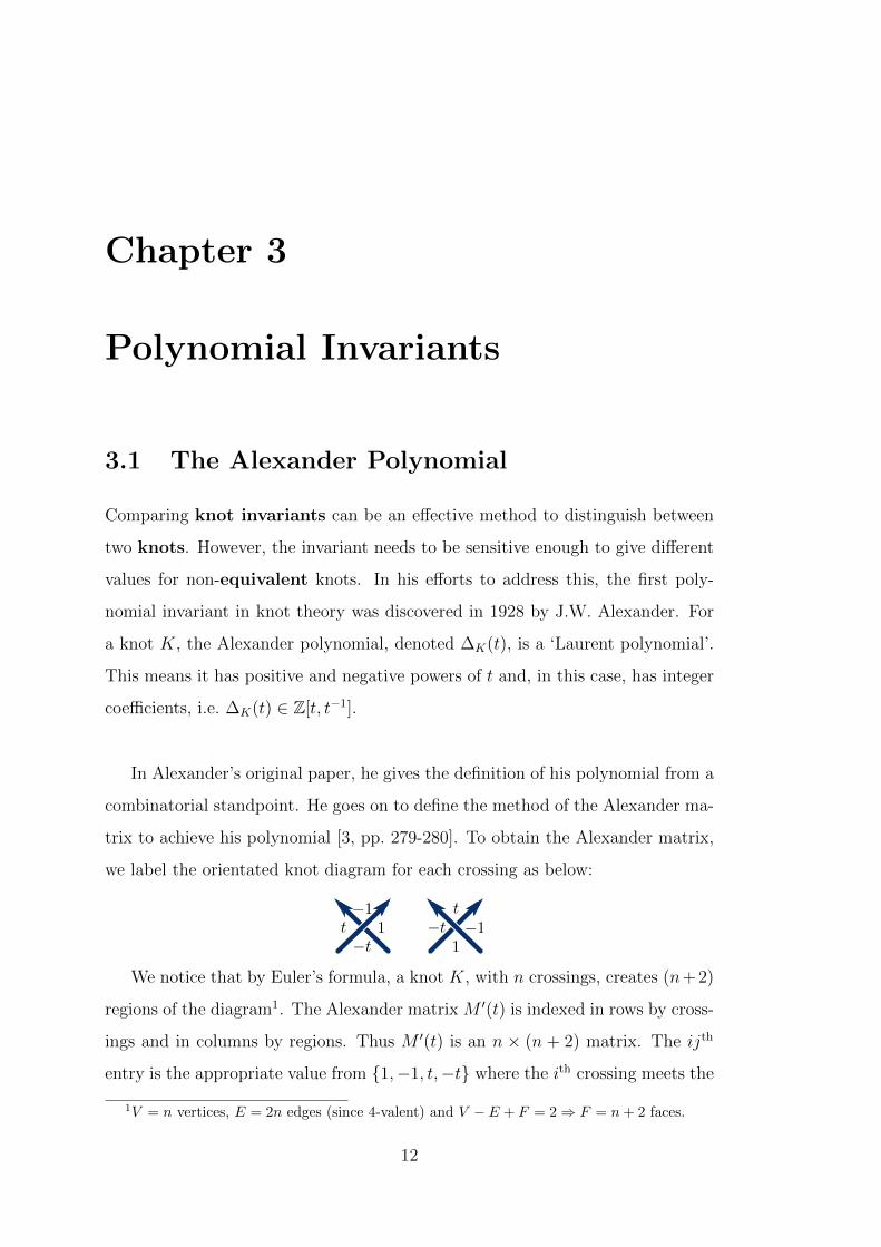
we label the orientated knot diagram for each crossing as below:

We notice that by Euler’s formula, a knot K, with n crossings, creates (n+ 2)

regions of the diagram1. The Alexander matrix M ′(t) is indexed in rows by cross-

ings and in columns by regions. Thus M ′(t) is an n × (n + 2) matrix. The ijth

entry is the appropriate value from {1,−1, t,−t} where the ith crossing meets the

1V = n vertices, E = 2n edges (since 4-valent) and V − E + F = 2⇒ F = n+ 2 faces.

12

3.1. The Alexander Polynomial

jth region, or takes the value zero if the region does not touch that crossing.

Next, we remove any two columns from the matrix which correspond to adja-

cent regions2 to obtain the reduced Alexander matrix, M(t). From the remaining

n× n matrix, we then find the determinant det(M(t)).

The final stage is to factor out the largest possible power of t and multiply

by ±1 to ensure the term of lowest degree in the determinant is a positive con-

stant, just for convention. An alternative convention is to then divide through

by ts/2 where s is the highest power of t. This gives a palindromic polynomial.

The resulting expressions are Alexander polynomials, ∆K(t). Note that if two

Alexander polynomials differ by a factor of ±tm we consider them to be equiva-

lent. A calculation of the Alexander polynomial is given in Chapter 5.

It is important to note that the determinant of the reduced matrix is depen-

dent on the choice made as to which two columns are removed. This consequently

adds some ambiguity to the answer, however it will only change within a factor

of ±tm for some m ∈ Z as shown in Theorem 1.

Despite the advancements that the Alexander polynomial made, it is still not

a complete invariant as it cannot successfully distinguish between all knots, in

particular the unknot, which has Alexander polynomial ∆01(t) = 1. This is

because nontrivial knots exist with the same Alexander polynomial, such as the

Kinoshita-Terasaka knot [15, p. 151] which has crossing number 11.

3.1.1 Proof that ∆K(t) is well defined

Theorem 1. The following three choices do not affect the determinant |M | by

more than a factor of ±tm:

1. The orientation of the knot.

2. The way that the regions and crossings in the knot are indexed.

2two regions which share an edge.

13

3. POLYNOMIAL INVARIANTS

3. The two adjacent columns that are removed.

Proof. Let us examine the effect of each case individually.

1. The orientation of the knot.

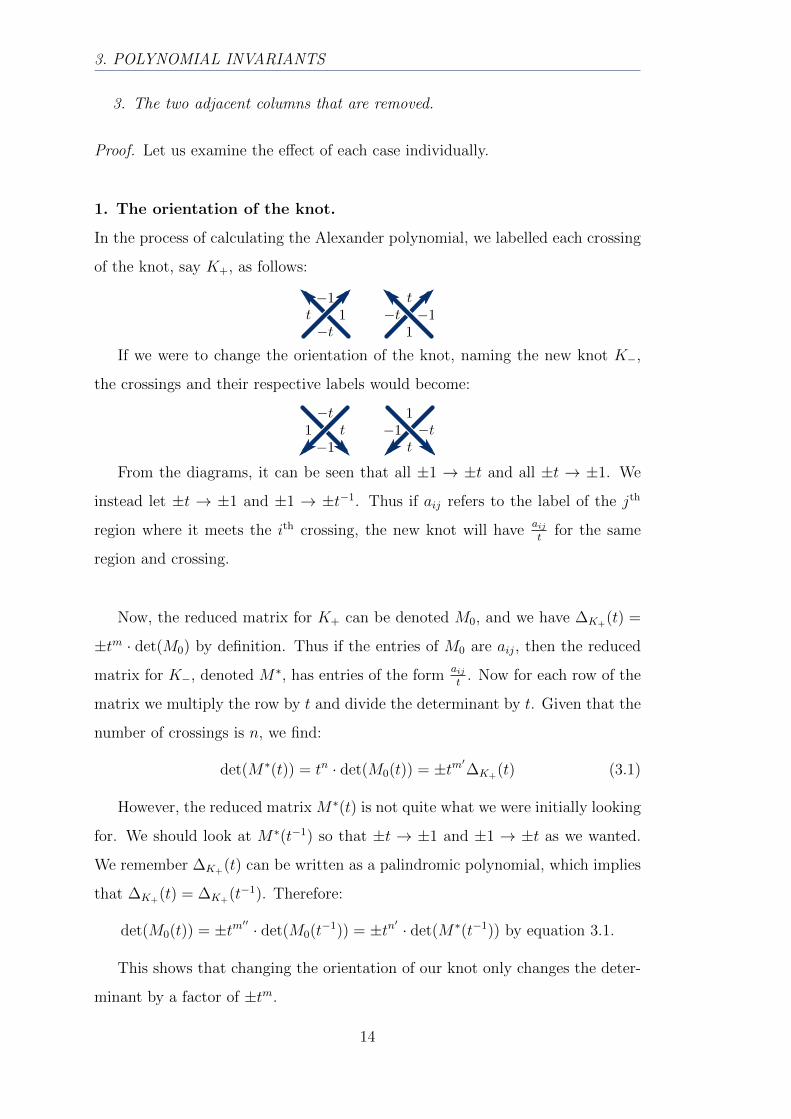
In the process of calculating the Alexander polynomial, we labelled each crossing

of the knot, say K+, as follows:

If we were to change the orientation of the knot, naming the new knot K−,

the crossings and their respective labels would become:

From the diagrams, it can be seen that all ±1 → ±t and all ±t → ±1. We

instead let ±t → ±1 and ±1 → ±t−1. Thus if aij refers to the label of the jth

region where it meets the ith crossing, the new knot will haveaijt

for the same

region and crossing.

Now, the reduced matrix for K+ can be denoted M0, and we have ∆K+(t) =

±tm · det(M0) by definition. Thus if the entries of M0 are aij, then the reduced

matrix for K−, denoted M∗, has entries of the formaijt

. Now for each row of the

matrix we multiply the row by t and divide the determinant by t. Given that the

number of crossings is n, we find:

det(M∗(t)) = tn · det(M0(t)) = ±tm′∆K+(t) (3.1)

However, the reduced matrix M∗(t) is not quite what we were initially looking

for. We should look at M∗(t−1) so that ±t → ±1 and ±1 → ±t as we wanted.

We remember ∆K+(t) can be written as a palindromic polynomial, which implies

that ∆K+(t) = ∆K+(t−1). Therefore:

det(M0(t)) = ±tm′′ · det(M0(t−1)) = ±tn′ · det(M∗(t−1)) by equation 3.1.

This shows that changing the orientation of our knot only changes the deter-

minant by a factor of ±tm.

14

3.1. The Alexander Polynomial

2. Indexing the regions and crossings in the knot

Altering the way that the regions and crossings in the knot are indexed only

alters the order of the rows and columns of the matrix M(t). Swapping rows or

columns in the matrix only multiplies the determinant by ±1 and thus the way

the regions and crossing in the knot are indexed only affects the determinant by

a factor of ±1.

3. Removing two adjacent columns [3, pp. 280-281]

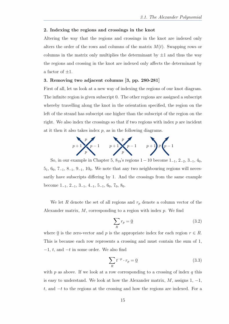
First of all, let us look at a new way of indexing the regions of our knot diagram.

The infinite region is given subscript 0. The other regions are assigned a subscript

whereby travelling along the knot in the orientation specified, the region on the

left of the strand has subscript one higher than the subscript of the region on the

right. We also index the crossings so that if two regions with index p are incident

at it then it also takes index p, as in the following diagrams.

So, in our example in Chapter 5, 819’s regions 1−10 become 1−1, 2−2, 3−1, 40,

51, 60, 7−1, 8−1, 9−1, 100. We note that any two neighbouring regions will neces-

sarily have subscripts differing by 1. And the crossings from the same example

become 1−1, 2−1, 3−1, 4−1, 5−1, 60, 70, 80.

We let R denote the set of all regions and rp denote a column vector of the

Alexander matrix, M , corresponding to a region with index p. We find∑R

rp = 0 (3.2)

where 0 is the zero-vector and p is the appropriate index for each region r ∈ R.

This is because each row represents a crossing and must contain the sum of 1,

−1, t, and −t in some order. We also find∑R

t−p · rp = 0 (3.3)

with p as above. If we look at a row corresponding to a crossing of index q this

is easy to understand. We look at how the Alexander matrix, M , assigns 1, −1,

t, and −t to the regions at the crossing and how the regions are indexed. For a

15

3. POLYNOMIAL INVARIANTS

crossing of index q we sum either 1 · t−(q−1) − 1 · t−q + t · t−(q+1) − t · t−q = 0 or

1 · t−q − 1 · t−(q−1) + t · t−q − t · t−(q+1) = 0 if it is a positive or negative crossing

respectively. Combining equations 3.2 and 3.3 we get∑R

(t−p − 1) · rp = 0.

We see that for p = 0 we have (t0 − 1) · r0 for each r0 ∈ R but t0 − 1 = 0 so the

regions with index 0 disappear. Therefore, for any r∗ with index q we have

(t−q − 1) · r∗ = −∑

R\{r∗}

(t−p − 1) · rp.

We now define |Mpq(t)| = |Mqp(t)| to be the determinant of the reduced Alexander

matrix where we have removed a pair of columns with indices p, q for p 6= q. For

ease, let us rename the columns of M so that M = (v0, v1, . . . , vi, . . . , vj, . . . , vn).

We let v0, vi and vj have indices 0, q and s respectively. We call M0q the reduced

matrix with v0 and vi removed and call M0s the reduced matrix with v0 and vj

removed. We find

(t−s − 1) · |M0q| = |v1, . . . , vi−1, vi+1, . . . , (t−s − 1) · vj, . . . , vn|

= |v1, . . . , vi−1, vi+1, . . . ,−∑

R\{vj ,v0}

(t−p − 1) · rp, . . . , vn|,

and since the sum has multiples of all the other columns, they can be subtracted

without changing the determinant, leaving a multiple of vi:

= |v1, . . . , vi−1, vi+1, . . . ,−(t−q − 1) · vi, . . . , vn|

= (t−q − 1) · |v1, . . . , vi−1, vi+1, . . . ,−vi, . . . , vn|

= ±(t−q − 1) · |v1, . . . , vi, . . . , vj−1, vj+1, . . . , vn|

= ±(t−q − 1) · |M0s|

where, in each step, we have either multiplied a column by a constant, added mul-

tiples of other columns to a column, or re-ordered the columns, so as not to change

the determinant by more than a constant factor. Moreover, since the indices are

only determined up to an additive constant, we can replace 0 with p. Then

(tp−s − 1) · |Mpq| = ±(tp−q − 1) · |Mps|

(ts−r − 1) · |Msp| = ±(ts−p − 1) · |Msr|

16

3.1. The Alexander Polynomial

⇒ |Mpq| =±(tp−q − 1)

(tp−s − 1)· |Mps|

|Msp| =±(ts−p − 1)

(ts−r − 1)· |Msr|

⇒ |Mpq| =±(tp−q − 1) · (ts−p − 1)

(tp−s − 1) · (ts−r − 1)· |Msr|

=±ts−p · (tp−q − 1)

(ts−r − 1)· |Msr| .

In particular, if q = p+ 1, r = s+ 1, we find∣∣Mp(p+1)

∣∣ =±ts−p · (t−1 − 1)

(t−1 − 1)·∣∣Ms(s+1)

∣∣= ±ts−p ·

∣∣Ms(s+1)

∣∣ .We find that whichever two columns are removed, as long as they have indices dif-

fering by 1, (in particular, if they are neighbouring,) we find that the determinant

of the matrix is changed by at most a factor of ±tm.

We have checked that the only choices we can make in calculating ∆K(t) do

not change the polynomial by more than a factor of ±tm. Thus, the Alexander

polynomial is well defined up to sign and multiplication by powers of t.

3.1.2 Proof of Invariance

In order to prove invariance it must be shown that K ∼ K ′ ⇒ ∆K(t) = ∆K′(t).

Since K ∼ K ′ iff K and K ′ are related by a sequence of Reidemeister moves

it is enough to show that the Alexander polynomial remains unchanged by the

Reidemeister moves. Since the last few steps of the calculation are just ‘tidying

up’, we need only show that the determinants of the matrices are only different

by a factor of ±tm.

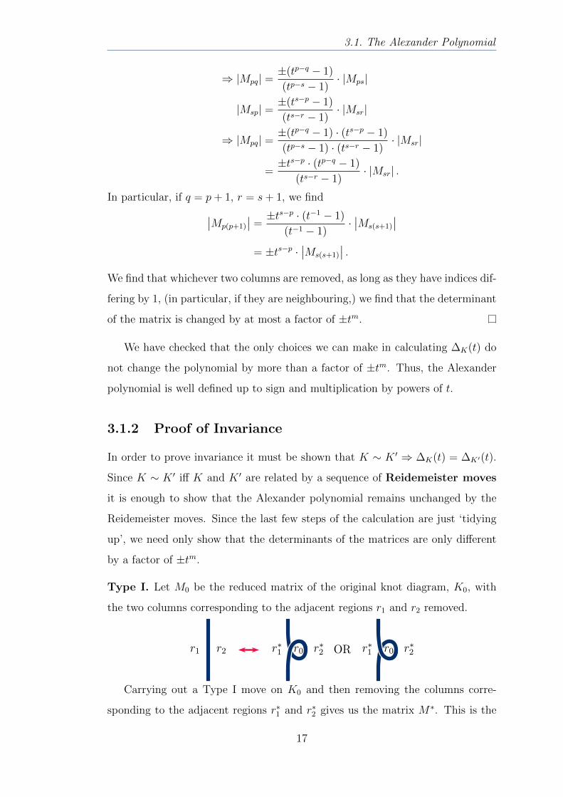
Type I. Let M0 be the reduced matrix of the original knot diagram, K0, with

the two columns corresponding to the adjacent regions r1 and r2 removed.

Carrying out a Type I move on K0 and then removing the columns corre-

sponding to the adjacent regions r∗1 and r∗2 gives us the matrix M∗. This is the

17

3. POLYNOMIAL INVARIANTS

same matrix as M0 but with one new row, for the new crossing, and one new

column, for the new region r0. The new row and column will contain all zeros

except for where they coincide, as r0 does not meet any other crossings and the

new crossing only meets regions r0, r∗1 and r∗2, two of which have been removed.

The non-zero entry will be any of {1,−1, t,−t}.

The determinant of the new reduced matrix M∗ is therefore:∣∣∣∣∣∣∣∣∣∣±tm 0 · · · 0

0M0

...0

∣∣∣∣∣∣∣∣∣∣= ±tm ·

∣∣∣∣∣∣∣∣∣∣1 0 · · · 0

0M0

...0

∣∣∣∣∣∣∣∣∣∣= ±tm ·

∣∣∣∣∣∣M0

∣∣∣∣∣∣ for m ∈ {0, 1}

As M∗ differs from M0 by at most a factor of ±tn, the polynomials yielded

from M0 and M∗ are equivalent. Thus, ∆K(t) is invariant under moves of Type I.

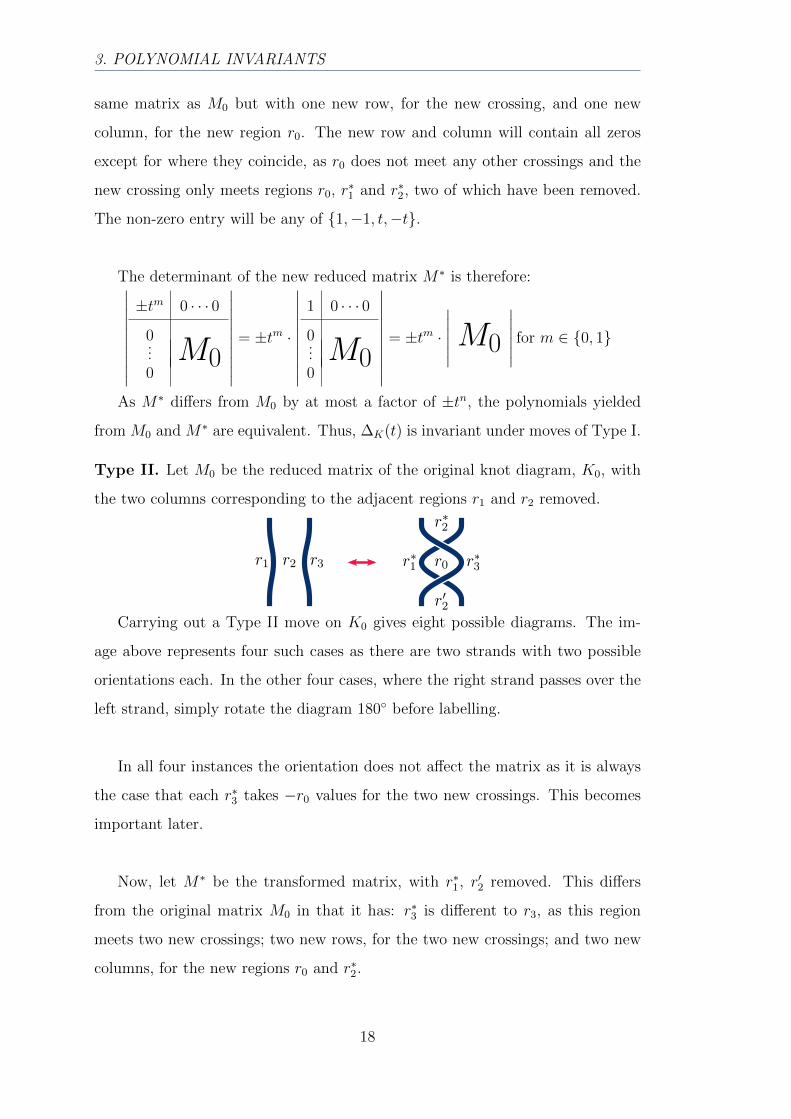
Type II. Let M0 be the reduced matrix of the original knot diagram, K0, with

the two columns corresponding to the adjacent regions r1 and r2 removed.

Carrying out a Type II move on K0 gives eight possible diagrams. The im-

age above represents four such cases as there are two strands with two possible

orientations each. In the other four cases, where the right strand passes over the

left strand, simply rotate the diagram 180◦ before labelling.

In all four instances the orientation does not affect the matrix as it is always

the case that each r∗3 takes −r0 values for the two new crossings. This becomes

important later.

Now, let M∗ be the transformed matrix, with r∗1, r′2 removed. This differs

from the original matrix M0 in that it has: r∗3 is different to r3, as this region

meets two new crossings; two new rows, for the two new crossings; and two new

columns, for the new regions r0 and r∗2.

18

3.1. The Alexander Polynomial

In M∗, if we now send r∗3 → r∗3 + r0 we do not change the determinant and we

obtain the original matrix M0 bordered by the two new rows and columns. This

is because r∗3 + r0 = original r3 and the other entries are not affected.∣∣∣∣∣∣∣∣∣∣∣∣∣

±tm ±tn 0 · · · 0

∓tm 0 0 · · · 0

0ξ M0

...0

∣∣∣∣∣∣∣∣∣∣∣∣∣=

∣∣∣∣∣∣∣∣∣∣∣∣∣

0 ±tn 0 · · · 0

∓tm 0 0 · · · 0

0ξ M0

...0

∣∣∣∣∣∣∣∣∣∣∣∣∣= ±tm′ ·

∣∣∣∣∣∣M0

∣∣∣∣∣∣In the first matrix we let the top row of M∗ represent the top crossing of

our image and the second row the lower crossing. Also, we let the first column

represent r0 and the second column r∗2. In r∗2 we write ξ for a potentially non-zero

column vector.

Now, in order to show M∗ and M0 are equivalent, we add the second row of

M∗ to the first as the two non-zero r0 entries must be the negation of each other.

Then we divide the first row by ±tn and the second row by ∓tm, whilst multi-

plying the determinant by both. Next we want to make the entries in ξ equal

zero. To do this we add multiples of the first row to all of the other rows. This

does not affect the rest of the matrix because all of the other entries in the row

are zero. Then we can drop the first and second rows and columns as required,

to get ±tm′ |M0|.

As M∗ differs from M0 by at most a factor of ±tm, the polynomials yielded

from M0 and M∗ are equivalent. Thus, ∆K(t) is invariant under moves of

Type II.

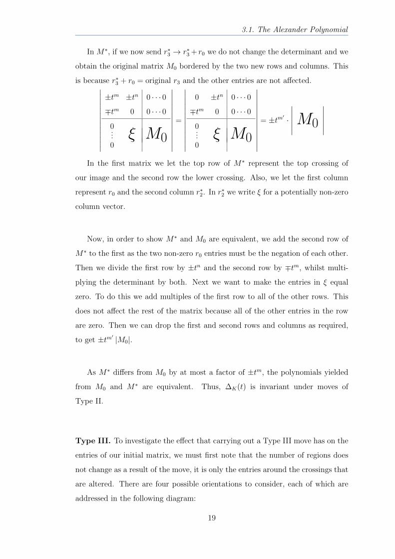
Type III. To investigate the effect that carrying out a Type III move has on the

entries of our initial matrix, we must first note that the number of regions does

not change as a result of the move, it is only the entries around the crossings that

are altered. There are four possible orientations to consider, each of which are

addressed in the following diagram:

19

3. POLYNOMIAL INVARIANTS

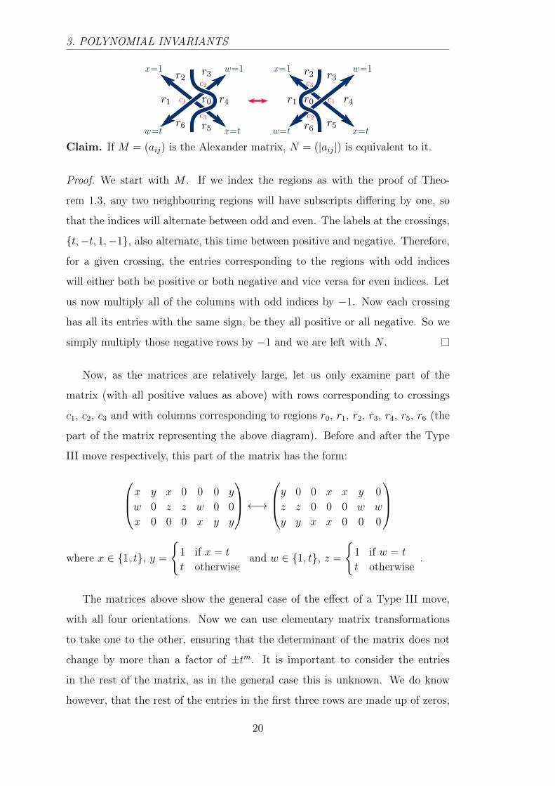
Claim. If M = (aij) is the Alexander matrix, N = (|aij|) is equivalent to it.

Proof. We start with M . If we index the regions as with the proof of Theo-

rem 1.3, any two neighbouring regions will have subscripts differing by one, so

that the indices will alternate between odd and even. The labels at the crossings,

{t,−t, 1,−1}, also alternate, this time between positive and negative. Therefore,

for a given crossing, the entries corresponding to the regions with odd indices

will either both be positive or both negative and vice versa for even indices. Let

us now multiply all of the columns with odd indices by −1. Now each crossing

has all its entries with the same sign, be they all positive or all negative. So we

simply multiply those negative rows by −1 and we are left with N .

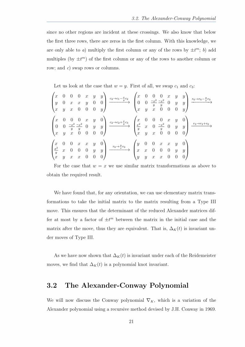
Now, as the matrices are relatively large, let us only examine part of the

matrix (with all positive values as above) with rows corresponding to crossings

c1, c2, c3 and with columns corresponding to regions r0, r1, r2, r3, r4, r5, r6 (the

part of the matrix representing the above diagram). Before and after the Type

III move respectively, this part of the matrix has the form:

x y x 0 0 0 y

w 0 z z w 0 0

x 0 0 0 x y y

←→y 0 0 x x y 0

z z 0 0 0 w w

y y x x 0 0 0

where x ∈ {1, t}, y =

{1 if x = t

t otherwiseand w ∈ {1, t}, z =

{1 if w = t

t otherwise.

The matrices above show the general case of the effect of a Type III move,

with all four orientations. Now we can use elementary matrix transformations

to take one to the other, ensuring that the determinant of the matrix does not

change by more than a factor of ±tm. It is important to consider the entries

in the rest of the matrix, as in the general case this is unknown. We do know

however, that the rest of the entries in the first three rows are made up of zeros,

20

3.2. The Alexander-Conway Polynomial

since no other regions are incident at these crossings. We also know that below

the first three rows, there are zeros in the first column. With this knowledge, we

are only able to a) multiply the first column or any of the rows by ±tm; b) add

multiples (by ±tm) of the first column or any of the rows to another column or

row; and c) swap rows or columns.

Let us look at the case that w = y. First of all, we swap c1 and c3:x 0 0 0 x y y

y 0 x x y 0 0

x y x 0 0 0 y

c2→c1−xyc2

−−−−−−→

x 0 0 0 x y y

0 0 −x2

y−x2

y0 y y

x y x 0 0 0 y

r6→r6− yxr0−−−−−−−→

x 0 0 0 x y 0

0 0 −x2

y−x2

y0 y y

x y x 0 0 0 0

c2→c2+xyc3

−−−−−−→

x 0 0 0 x y 0x2

yx 0 −x2

y0 y y

x y x 0 0 0 0

r3→r3+r0−−−−−−→

x 0 0 x x y 0x2

yx 0 0 0 y y

x y x x 0 0 0

r0→ yxr0−−−−−−→

y 0 0 x x y 0

x x 0 0 0 y y

y y x x 0 0 0

For the case that w = x we use similar matrix transformations as above to

obtain the required result.

We have found that, for any orientation, we can use elementary matrix trans-

formations to take the initial matrix to the matrix resulting from a Type III

move. This ensures that the determinant of the reduced Alexander matrices dif-

fer at most by a factor of ±tm between the matrix in the initial case and the

matrix after the move, thus they are equivalent. That is, ∆K(t) is invariant un-

der moves of Type III.

As we have now shown that ∆K(t) is invariant under each of the Reidemeister

moves, we find that ∆K(t) is a polynomial knot invariant.

3.2 The Alexander-Conway Polynomial

We will now discuss the Conway polynomial ∇K , which is a variation of the

Alexander polynomial using a recursive method devised by J.H. Conway in 1969.

21

3. POLYNOMIAL INVARIANTS

Conway himself stated that ‘∇K is just a disguised and normalized form of the

Alexander polynomial ∆K ’ [6, p. 337]. In fact ∇K can be defined completely by

different properties which we will investigate.

Definition. Given an oriented knot or link, K, there is an associated polynomial

∇K(z) that can be determined by means of the following two axioms [6, p. 338]:

Axiom 1. If 01 denotes the standard unknot, then ∇01(z) = 1.

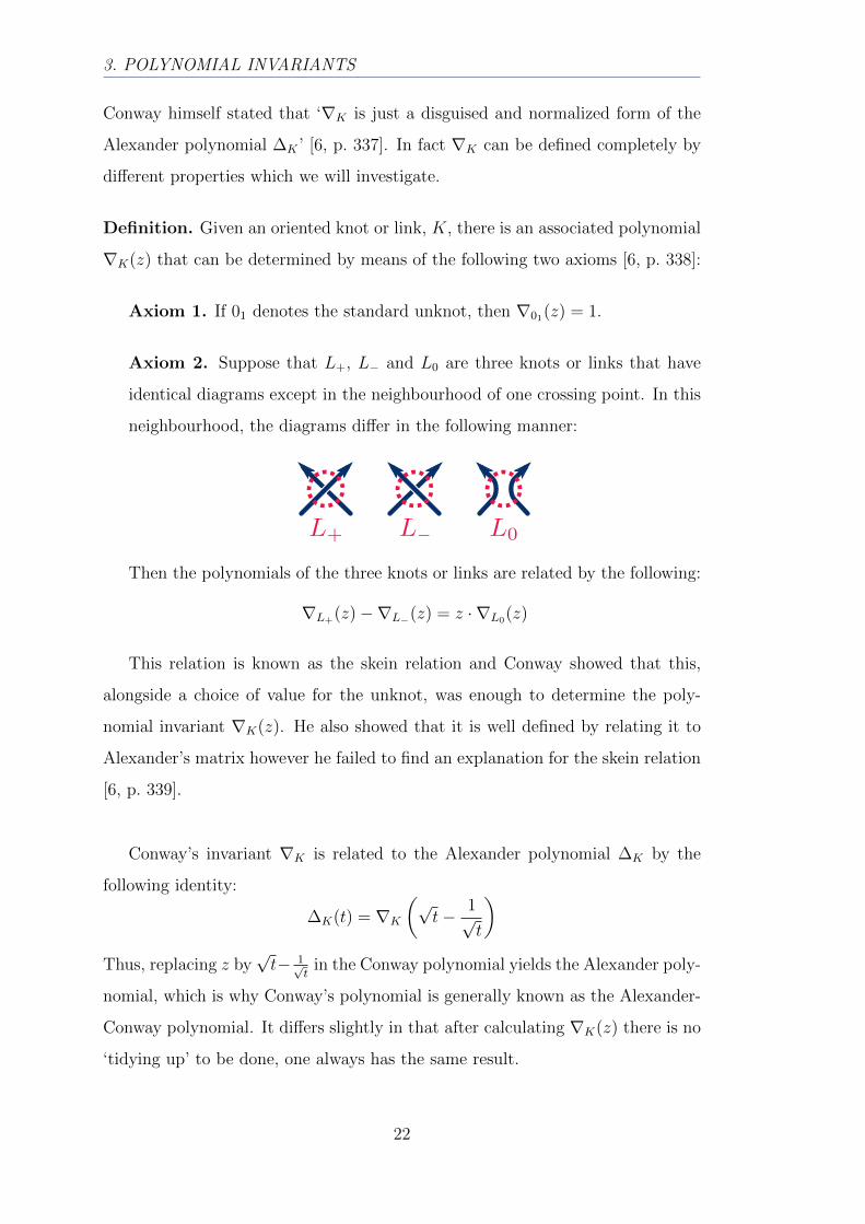
Axiom 2. Suppose that L+, L− and L0 are three knots or links that have

identical diagrams except in the neighbourhood of one crossing point. In this

neighbourhood, the diagrams differ in the following manner:

Then the polynomials of the three knots or links are related by the following:

∇L+(z)−∇L−(z) = z · ∇L0(z)

This relation is known as the skein relation and Conway showed that this,

alongside a choice of value for the unknot, was enough to determine the poly-

nomial invariant ∇K(z). He also showed that it is well defined by relating it to

Alexander’s matrix however he failed to find an explanation for the skein relation

[6, p. 339].

Conway’s invariant ∇K is related to the Alexander polynomial ∆K by the

following identity:

∆K(t) = ∇K

(√t− 1√

t

)Thus, replacing z by

√t− 1√

tin the Conway polynomial yields the Alexander poly-

nomial, which is why Conway’s polynomial is generally known as the Alexander-

Conway polynomial. It differs slightly in that after calculating ∇K(z) there is no

‘tidying up’ to be done, one always has the same result.

22

3.3. Further Polynomial Invariants

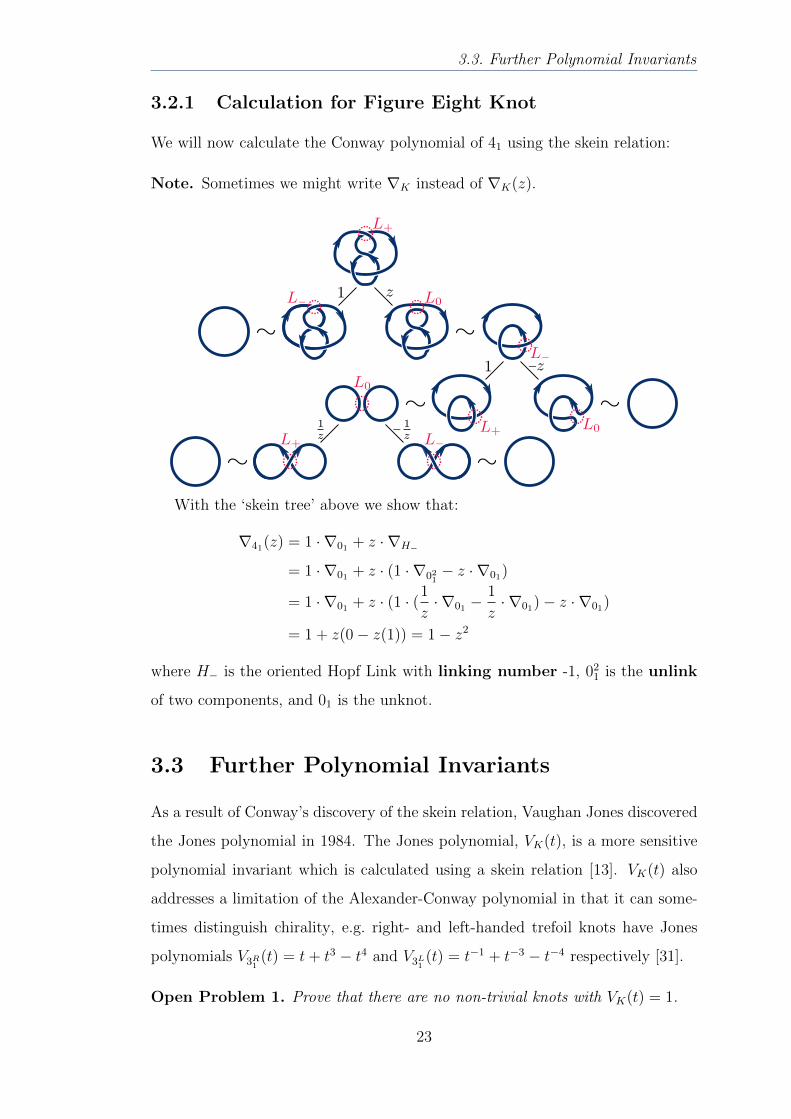
3.2.1 Calculation for Figure Eight Knot

We will now calculate the Conway polynomial of 41 using the skein relation:

Note. Sometimes we might write ∇K instead of ∇K(z).

With the ‘skein tree’ above we show that:

∇41(z) = 1 · ∇01 + z · ∇H−

= 1 · ∇01 + z · (1 · ∇021− z · ∇01)

= 1 · ∇01 + z · (1 · (1

z· ∇01 −

1

z· ∇01)− z · ∇01)

= 1 + z(0− z(1)) = 1− z2

where H− is the oriented Hopf Link with linking number -1, 021 is the unlink

of two components, and 01 is the unknot.

3.3 Further Polynomial Invariants

As a result of Conway’s discovery of the skein relation, Vaughan Jones discovered

the Jones polynomial in 1984. The Jones polynomial, VK(t), is a more sensitive

polynomial invariant which is calculated using a skein relation [13]. VK(t) also

addresses a limitation of the Alexander-Conway polynomial in that it can some-

times distinguish chirality, e.g. right- and left-handed trefoil knots have Jones

polynomials V3R1 (t) = t+ t3 − t4 and V3L1 (t) = t−1 + t−3 − t−4 respectively [31].

Open Problem 1. Prove that there are no non-trivial knots with VK(t) = 1.

23

3. POLYNOMIAL INVARIANTS

Although more sensitive, the Jones polynomial is by no means a complete

invariant and its discovery led to renewed exploration in this area. A year later,

a two-variable polynomial invariant was discovered, the HOMFLY (or HOM-

FLYPT) polynomial, which generalises both the Alexander and the Jones poly-

nomials. The HOMFLY polynomial is again more sensitive and opens further the

field of knot theory, however it is still not complete.

Open Problem 2. Find a complete knot invariant3.

3a knot invariant, say κ, such that κ(K) = κ(K ′)⇒ K ∼ K ′.

24

Chapter 4

Alternating Knots

Definition. An alternating knot is a knot for which there exists a knot diagram

in which crossings alternate between under and over as one travels around the

knot in a given direction. Note that not all knot diagrams of alternating knots

need be alternating [1, p. 7].

4.1 Examples

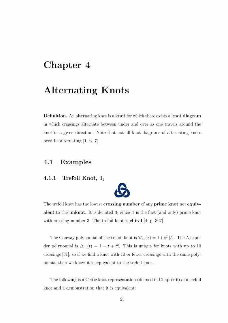
4.1.1 Trefoil Knot, 31

The trefoil knot has the lowest crossing number of any prime knot not equiv-

alent to the unknot. It is denoted 31 since it is the first (and only) prime knot

with crossing number 3. The trefoil knot is chiral [4, p. 367].

The Conway polynomial of the trefoil knot is ∇31(z) = 1+z2 [5]. The Alexan-

der polynomial is ∆31(t) = 1 − t + t2. This is unique for knots with up to 10

crossings [31], so if we find a knot with 10 or fewer crossings with the same poly-

nomial then we know it is equivalent to the trefoil knot.

The following is a Celtic knot representation (defined in Chapter 6) of a trefoil

knot and a demonstration that it is equivalent:

25

4. ALTERNATING KNOTS

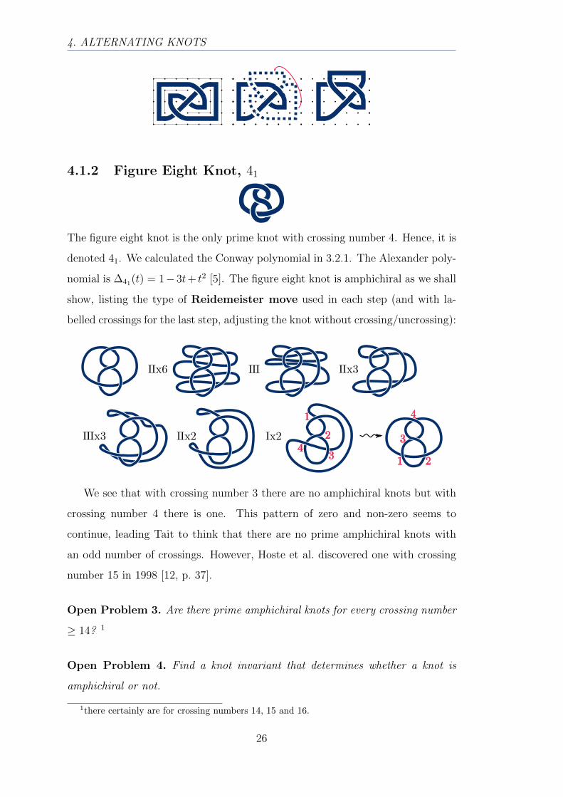
4.1.2 Figure Eight Knot, 41

The figure eight knot is the only prime knot with crossing number 4. Hence, it is

denoted 41. We calculated the Conway polynomial in 3.2.1. The Alexander poly-

nomial is ∆41(t) = 1−3t+ t2 [5]. The figure eight knot is amphichiral as we shall

show, listing the type of Reidemeister move used in each step (and with la-

belled crossings for the last step, adjusting the knot without crossing/uncrossing):

We see that with crossing number 3 there are no amphichiral knots but with

crossing number 4 there is one. This pattern of zero and non-zero seems to

continue, leading Tait to think that there are no prime amphichiral knots with

an odd number of crossings. However, Hoste et al. discovered one with crossing

number 15 in 1998 [12, p. 37].

Open Problem 3. Are there prime amphichiral knots for every crossing number

≥ 14? 1

Open Problem 4. Find a knot invariant that determines whether a knot is

amphichiral or not.

1there certainly are for crossing numbers 14, 15 and 16.

26

4.2. Properties

4.2 Properties

Alternating knots have many special properties. Looking at knots with low cross-

ing numbers, it can seem as if almost all knots are alternating. However, with

crossing number 13 there are more non-alternating prime knots than alternating

prime knots. And with crossing number 16 there are well over twice as many

non-alternating prime knots than alternating prime knots. In fact it has been

conjectured that the proportion of alternating knots tends exponentially to zero

as the crossing number increases [12, p. 36].

Probably the most striking properties unique to alternating knots, are those

conjectured by Tait in the 1870s.

Tait’s Conjectures [12, p. 35].

1. Reduced alternating knot diagrams have the minimal number of crossings.

2. Any two equivalent reduced alternating knot diagrams have equal writhe.

3. Any two equivalent reduced alternating knot diagrams are related by a suc-

cession of flypes.

It was not until Jones developed his polynomial over 100 years later [13], that

any of these conjectures were solved. In 1987, Kauffman, Murasugi and Thistleth-

waite proved the first and second conjectures using the Jones polynomial (and

Kauffman polynomial) [21], then four years later Menasco and Thistlethwaite

proved the third conjecture [18].

There are two other significant properties relating to the Alexander polyno-

mial of alternating knots.

Properties of Alexander polynomial.

1. If K is an alternating knot, all coefficients of ∆K(t) are non-zero.

2. If K is an alternating knot, the coefficients of ∆K(t) are alternating 2.

2a polynomial∑ant

n is alternating iff (−1)i+jaiaj ≥ 0

27

4. ALTERNATING KNOTS

The first theorem was proven by Murasugi in 1958 [20, p. 181] and the second

by Crowell in 1959 [7, p. 262].

We can use Tait’s first conjecture to prove another property of alternating

knots.

Theorem 2. Alternating knots are adequate3 knots.

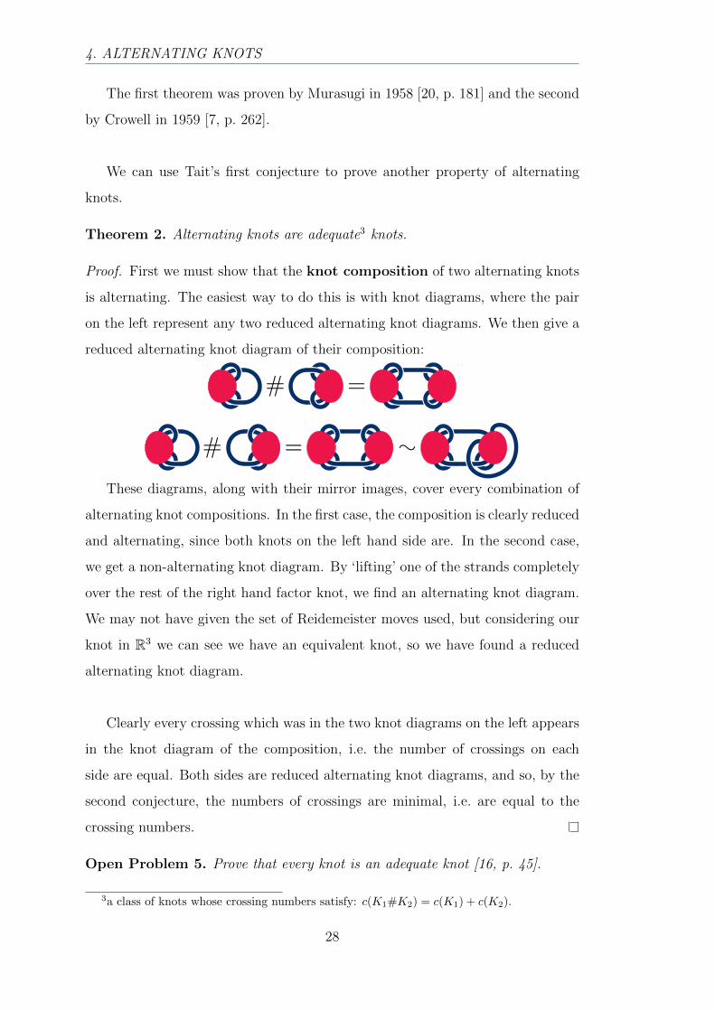
Proof. First we must show that the knot composition of two alternating knots

is alternating. The easiest way to do this is with knot diagrams, where the pair

on the left represent any two reduced alternating knot diagrams. We then give a

reduced alternating knot diagram of their composition:

These diagrams, along with their mirror images, cover every combination of

alternating knot compositions. In the first case, the composition is clearly reduced

and alternating, since both knots on the left hand side are. In the second case,

we get a non-alternating knot diagram. By ‘lifting’ one of the strands completely

over the rest of the right hand factor knot, we find an alternating knot diagram.

We may not have given the set of Reidemeister moves used, but considering our

knot in R3 we can see we have an equivalent knot, so we have found a reduced

alternating knot diagram.

Clearly every crossing which was in the two knot diagrams on the left appears

in the knot diagram of the composition, i.e. the number of crossings on each

side are equal. Both sides are reduced alternating knot diagrams, and so, by the

second conjecture, the numbers of crossings are minimal, i.e. are equal to the

crossing numbers.

Open Problem 5. Prove that every knot is an adequate knot [16, p. 45].

3a class of knots whose crossing numbers satisfy: c(K1#K2) = c(K1) + c(K2).

28

Chapter 5

Non-alternating Knots

Definition. A non-alternating knot is any knot which is not an alternating knot.

That is, a non-alternating knot is a knot for which there does not exist a knot

diagram in which crossings alternate between under- and over-passes.

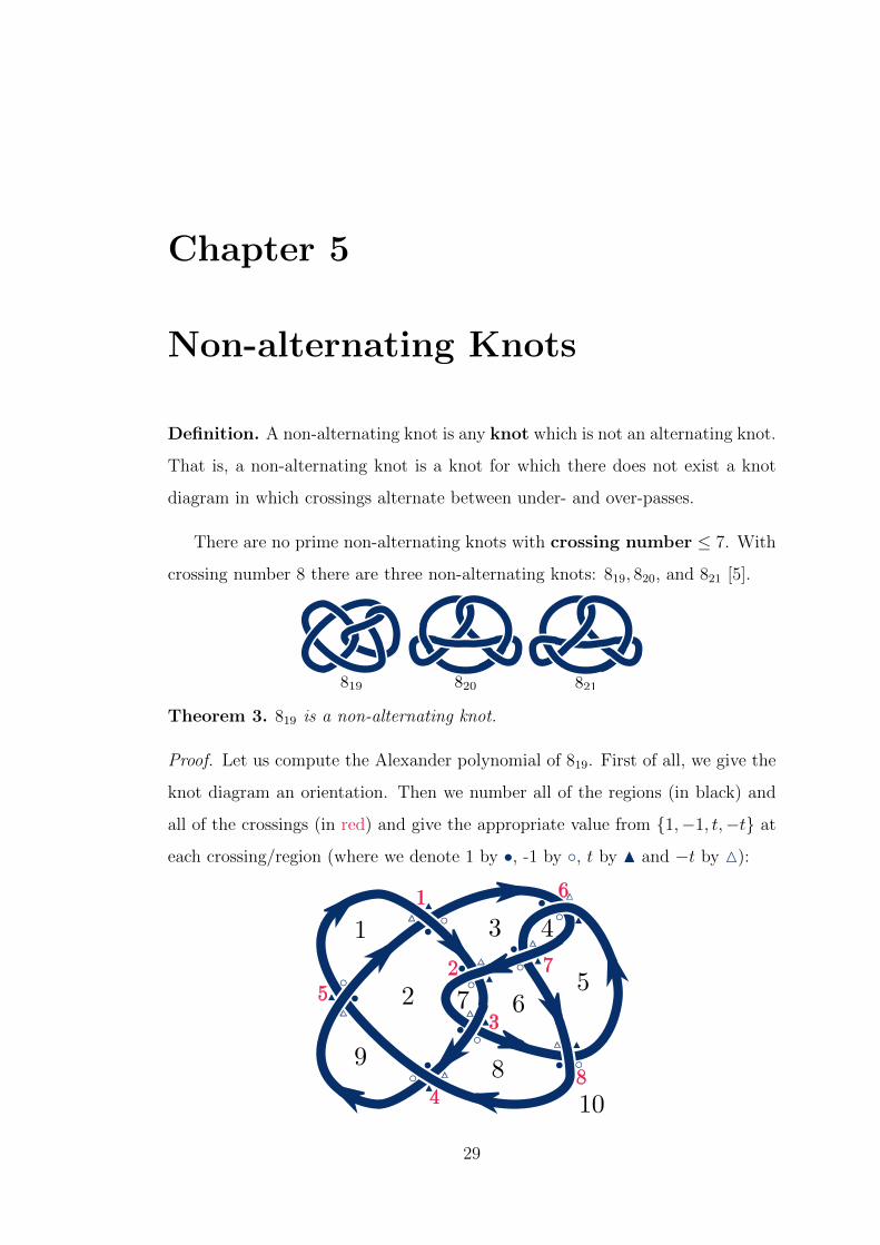
There are no prime non-alternating knots with crossing number ≤ 7. With

crossing number 8 there are three non-alternating knots: 819, 820, and 821 [5].

Theorem 3. 819 is a non-alternating knot.

Proof. Let us compute the Alexander polynomial of 819. First of all, we give the

knot diagram an orientation. Then we number all of the regions (in black) and

all of the crossings (in red) and give the appropriate value from {1,−1, t,−t} at

each crossing/region (where we denote 1 by •, -1 by ◦, t by N and −t by M):

29

5. NON-ALTERNATING KNOTS

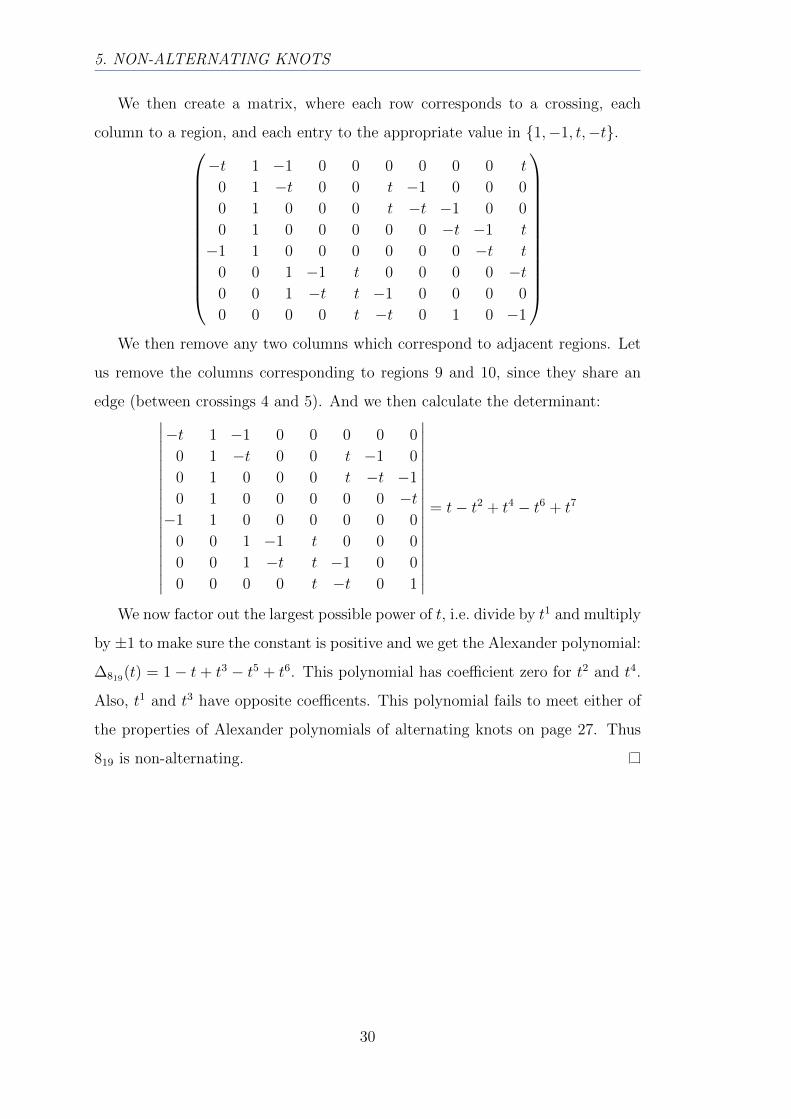
We then create a matrix, where each row corresponds to a crossing, each

column to a region, and each entry to the appropriate value in {1,−1, t,−t}.

−t 1 −1 0 0 0 0 0 0 t

0 1 −t 0 0 t −1 0 0 0

0 1 0 0 0 t −t −1 0 0

0 1 0 0 0 0 0 −t −1 t

−1 1 0 0 0 0 0 0 −t t

0 0 1 −1 t 0 0 0 0 −t0 0 1 −t t −1 0 0 0 0

0 0 0 0 t −t 0 1 0 −1

We then remove any two columns which correspond to adjacent regions. Let

us remove the columns corresponding to regions 9 and 10, since they share an

edge (between crossings 4 and 5). And we then calculate the determinant:∣∣∣∣∣∣∣∣∣∣∣∣∣∣∣∣∣∣

−t 1 −1 0 0 0 0 0

0 1 −t 0 0 t −1 0

0 1 0 0 0 t −t −1

0 1 0 0 0 0 0 −t−1 1 0 0 0 0 0 0

0 0 1 −1 t 0 0 0

0 0 1 −t t −1 0 0

0 0 0 0 t −t 0 1

∣∣∣∣∣∣∣∣∣∣∣∣∣∣∣∣∣∣= t− t2 + t4 − t6 + t7

We now factor out the largest possible power of t, i.e. divide by t1 and multiply

by ±1 to make sure the constant is positive and we get the Alexander polynomial:

∆819(t) = 1− t + t3 − t5 + t6. This polynomial has coefficient zero for t2 and t4.

Also, t1 and t3 have opposite coefficents. This polynomial fails to meet either of

the properties of Alexander polynomials of alternating knots on page 27. Thus

819 is non-alternating.

30

Chapter 6

Celtic Knots

Note. In this chapter we will sometimes use graph when we mean multigraph1 or

pseudograph2. Also, we often use knot instead of link. However, we rarely need

to restrict ourselves to one component.

6.1 What is a Celtic knot?

Celtic knots are stylized, interlaced patterns, representing ropes or threads tied

in a knot. To be strictly accurate, they are mis-named. They also appear in

the art of various other peoples including Romans, Vikings and Saxons. Gen-

erally, like our mathematical knots, they have no ends. In this case, they can

also be called Gordian knots, due to an ancient Greek myth. As the legend goes,

it was said that the person who untied Gordius’ knot would rule all of Asia. It

remained unsolved for many years, resisting all attempted solutions until 333BC

when Alexander the Great cut it through with a sword.

For the purposes of this paper we shall look at certain kinds of Celtic knots

that are drawn on a grid of dots. From now on we shall speak of Celtic knots as

if they are all of this kind.

Definition. A Celtic knot is a link diagram created by a boundary, barriers

(horizontal or vertical lines going from one dot to another, that will ‘reflect’ the

1a graph which permits multiple edges between two vertices.2a multigraph which allows loops (an edge starting and finishing at one vertex).

31

6. CELTIC KNOTS

strands) and tiles, in the following way.

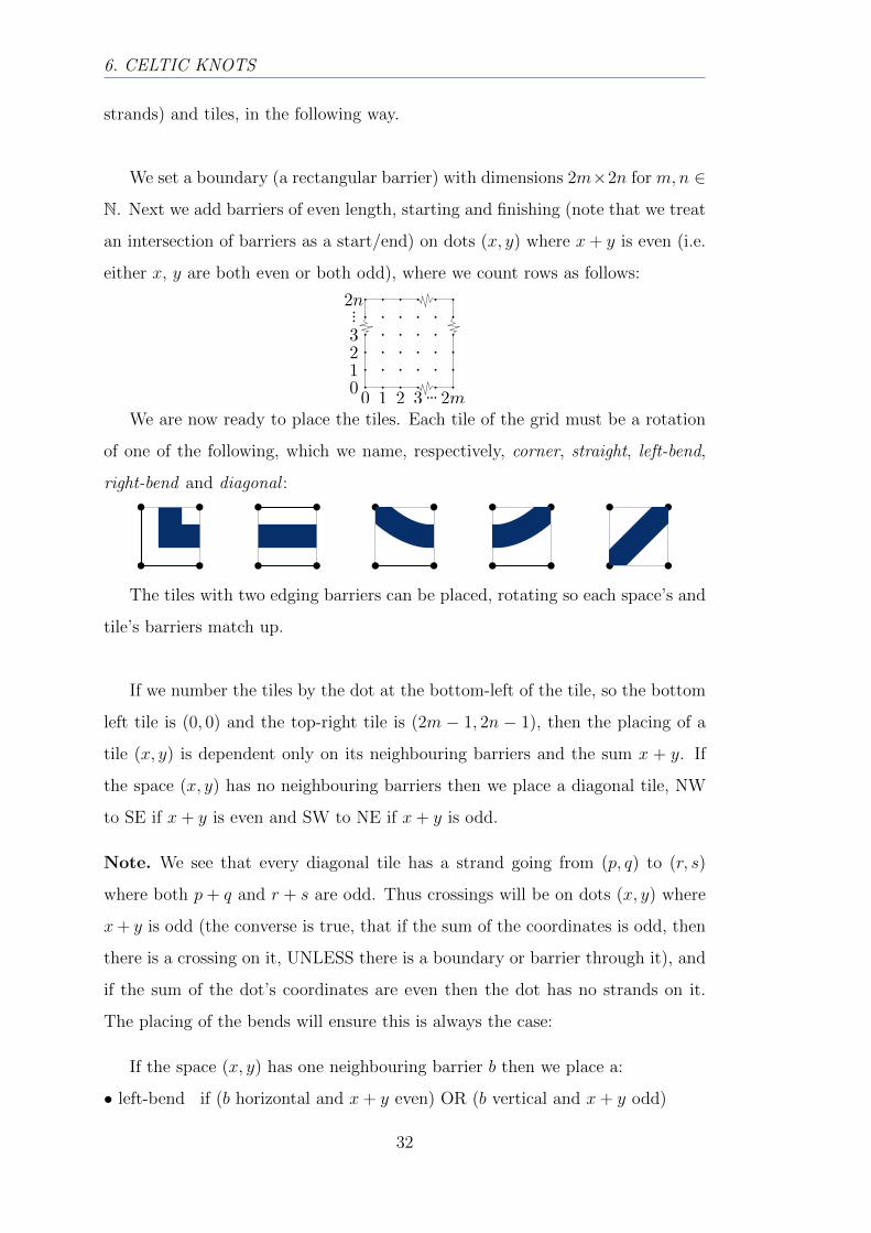
We set a boundary (a rectangular barrier) with dimensions 2m×2n for m,n ∈

N. Next we add barriers of even length, starting and finishing (note that we treat

an intersection of barriers as a start/end) on dots (x, y) where x+ y is even (i.e.

either x, y are both even or both odd), where we count rows as follows:

We are now ready to place the tiles. Each tile of the grid must be a rotation

of one of the following, which we name, respectively, corner, straight, left-bend,

right-bend and diagonal :

The tiles with two edging barriers can be placed, rotating so each space’s and

tile’s barriers match up.

If we number the tiles by the dot at the bottom-left of the tile, so the bottom

left tile is (0, 0) and the top-right tile is (2m − 1, 2n − 1), then the placing of a

tile (x, y) is dependent only on its neighbouring barriers and the sum x + y. If

the space (x, y) has no neighbouring barriers then we place a diagonal tile, NW

to SE if x+ y is even and SW to NE if x+ y is odd.

Note. We see that every diagonal tile has a strand going from (p, q) to (r, s)

where both p+ q and r + s are odd. Thus crossings will be on dots (x, y) where

x+ y is odd (the converse is true, that if the sum of the coordinates is odd, then

there is a crossing on it, UNLESS there is a boundary or barrier through it), and

if the sum of the dot’s coordinates are even then the dot has no strands on it.

The placing of the bends will ensure this is always the case:

If the space (x, y) has one neighbouring barrier b then we place a:

• left-bend if (b horizontal and x+ y even) OR (b vertical and x+ y odd)

32

6.2. Construction

• right-bend if (b horizontal and x+ y odd) OR (b vertical and x+ y even)

rotating so that the space’s and tile’s barriers match up.

We then put NW to SE over-crossings on the odd rows and SW to NE over-

crossings on the even rows.

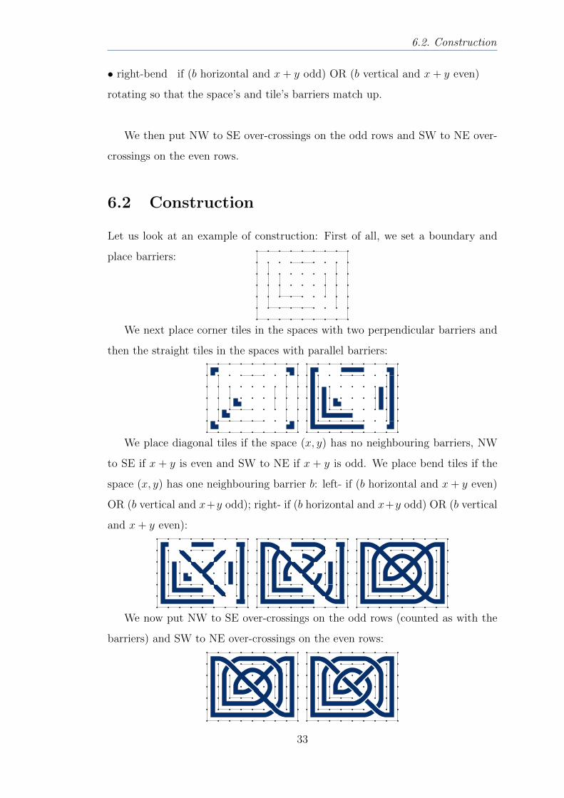
6.2 Construction

Let us look at an example of construction: First of all, we set a boundary and

place barriers:

We next place corner tiles in the spaces with two perpendicular barriers and

then the straight tiles in the spaces with parallel barriers:

We place diagonal tiles if the space (x, y) has no neighbouring barriers, NW

to SE if x + y is even and SW to NE if x + y is odd. We place bend tiles if the

space (x, y) has one neighbouring barrier b: left- if (b horizontal and x+ y even)

OR (b vertical and x+y odd); right- if (b horizontal and x+y odd) OR (b vertical

and x+ y even):

We now put NW to SE over-crossings on the odd rows (counted as with the

barriers) and SW to NE over-crossings on the even rows:

33

6. CELTIC KNOTS

6.3 Celtic Knots vs. Alternating Knots

6.3.1 Celtic Knots

Theorem 4. Every Celtic knot is alternating.

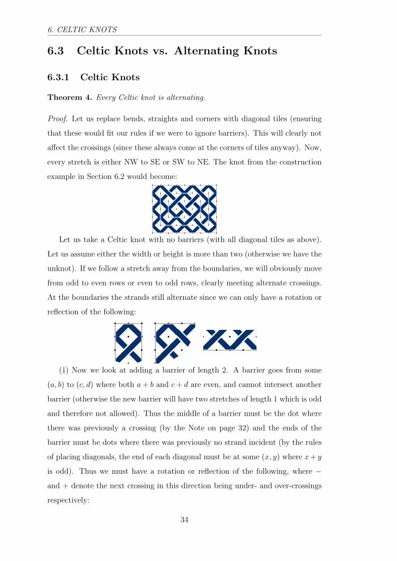
Proof. Let us replace bends, straights and corners with diagonal tiles (ensuring

that these would fit our rules if we were to ignore barriers). This will clearly not

affect the crossings (since these always come at the corners of tiles anyway). Now,

every stretch is either NW to SE or SW to NE. The knot from the construction

example in Section 6.2 would become:

Let us take a Celtic knot with no barriers (with all diagonal tiles as above).

Let us assume either the width or height is more than two (otherwise we have the

unknot). If we follow a stretch away from the boundaries, we will obviously move

from odd to even rows or even to odd rows, clearly meeting alternate crossings.

At the boundaries the strands still alternate since we can only have a rotation or

reflection of the following:

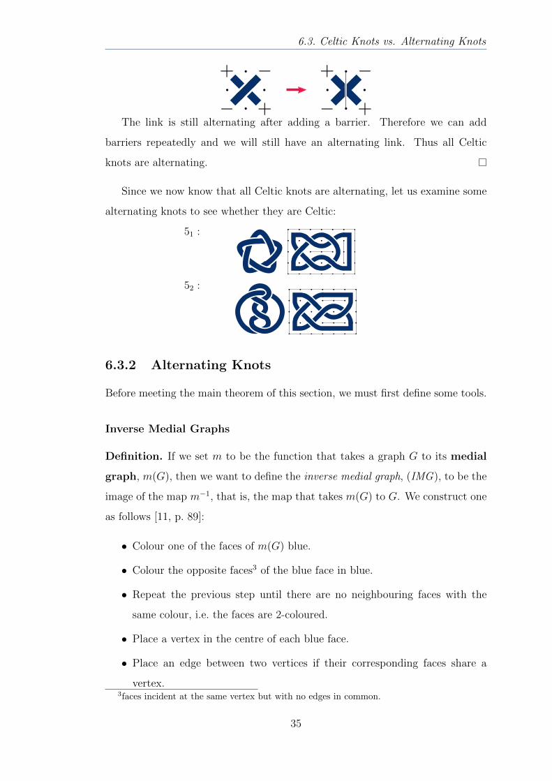
(†) Now we look at adding a barrier of length 2. A barrier goes from some

(a, b) to (c, d) where both a+ b and c+ d are even, and cannot intersect another

barrier (otherwise the new barrier will have two stretches of length 1 which is odd

and therefore not allowed). Thus the middle of a barrier must be the dot where

there was previously a crossing (by the Note on page 32) and the ends of the

barrier must be dots where there was previously no strand incident (by the rules

of placing diagonals, the end of each diagonal must be at some (x, y) where x+ y

is odd). Thus we must have a rotation or reflection of the following, where −

and + denote the next crossing in this direction being under- and over-crossings

respectively:

34

6.3. Celtic Knots vs. Alternating Knots

The link is still alternating after adding a barrier. Therefore we can add

barriers repeatedly and we will still have an alternating link. Thus all Celtic

knots are alternating.

Since we now know that all Celtic knots are alternating, let us examine some

alternating knots to see whether they are Celtic:

51 :

52 :

6.3.2 Alternating Knots

Before meeting the main theorem of this section, we must first define some tools.

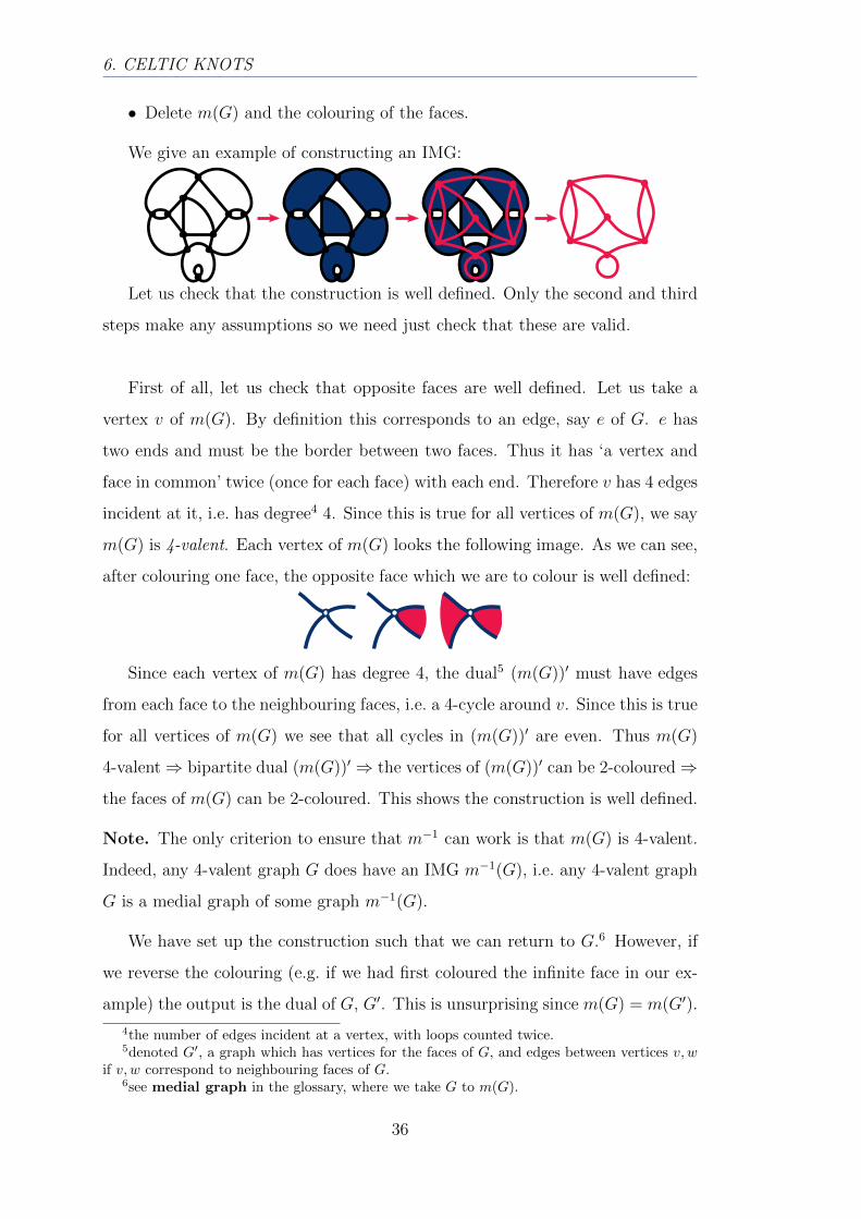
Inverse Medial Graphs

Definition. If we set m to be the function that takes a graph G to its medial

graph, m(G), then we want to define the inverse medial graph, (IMG), to be the

image of the map m−1, that is, the map that takes m(G) to G. We construct one

as follows [11, p. 89]:

• Colour one of the faces of m(G) blue.

• Colour the opposite faces3 of the blue face in blue.

• Repeat the previous step until there are no neighbouring faces with the

same colour, i.e. the faces are 2-coloured.

• Place a vertex in the centre of each blue face.

• Place an edge between two vertices if their corresponding faces share a

vertex.3faces incident at the same vertex but with no edges in common.

35

6. CELTIC KNOTS

• Delete m(G) and the colouring of the faces.

We give an example of constructing an IMG:

Let us check that the construction is well defined. Only the second and third

steps make any assumptions so we need just check that these are valid.

First of all, let us check that opposite faces are well defined. Let us take a

vertex v of m(G). By definition this corresponds to an edge, say e of G. e has

two ends and must be the border between two faces. Thus it has ‘a vertex and

face in common’ twice (once for each face) with each end. Therefore v has 4 edges

incident at it, i.e. has degree4 4. Since this is true for all vertices of m(G), we say

m(G) is 4-valent. Each vertex of m(G) looks the following image. As we can see,

after colouring one face, the opposite face which we are to colour is well defined:

Since each vertex of m(G) has degree 4, the dual5 (m(G))′ must have edges

from each face to the neighbouring faces, i.e. a 4-cycle around v. Since this is true

for all vertices of m(G) we see that all cycles in (m(G))′ are even. Thus m(G)

4-valent⇒ bipartite dual (m(G))′ ⇒ the vertices of (m(G))′ can be 2-coloured⇒

the faces of m(G) can be 2-coloured. This shows the construction is well defined.

Note. The only criterion to ensure that m−1 can work is that m(G) is 4-valent.

Indeed, any 4-valent graph G does have an IMG m−1(G), i.e. any 4-valent graph

G is a medial graph of some graph m−1(G).

We have set up the construction such that we can return to G.6 However, if

we reverse the colouring (e.g. if we had first coloured the infinite face in our ex-

ample) the output is the dual of G, G′. This is unsurprising since m(G) = m(G′).

4the number of edges incident at a vertex, with loops counted twice.5denoted G′, a graph which has vertices for the faces of G, and edges between vertices v, w

if v, w correspond to neighbouring faces of G.6see medial graph in the glossary, where we take G to m(G).

36

6.3. Celtic Knots vs. Alternating Knots

Since we started out by 2-colouring the faces of m(G) we cannot get any other

possibilities for m−1(m(G)).

We find that we have not necessarily found the map that takes m(G) to G,

as it may take it to G′, i.e. m−1(m(G)) = G OR G′. However, we have found a

map such that m(m−1(G)) = G.

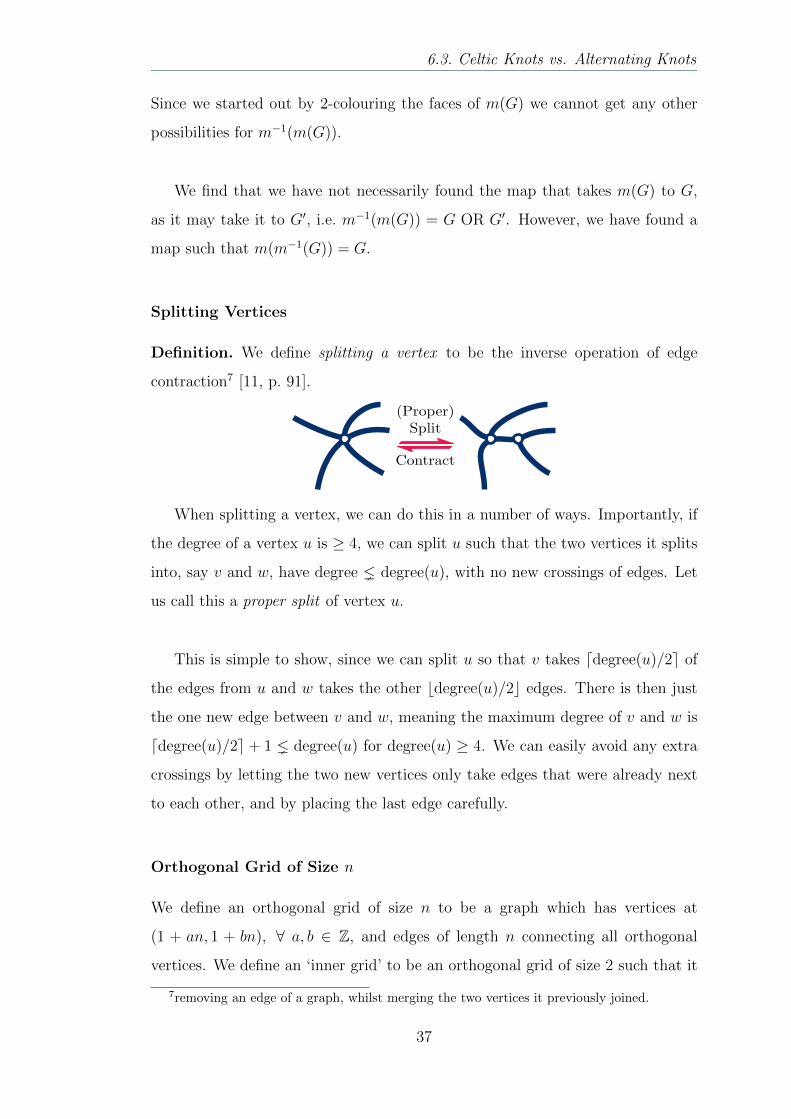
Splitting Vertices

Definition. We define splitting a vertex to be the inverse operation of edge

contraction7 [11, p. 91].

When splitting a vertex, we can do this in a number of ways. Importantly, if

the degree of a vertex u is ≥ 4, we can split u such that the two vertices it splits

into, say v and w, have degree � degree(u), with no new crossings of edges. Let

us call this a proper split of vertex u.

This is simple to show, since we can split u so that v takes ddegree(u)/2e of

the edges from u and w takes the other bdegree(u)/2c edges. There is then just

the one new edge between v and w, meaning the maximum degree of v and w is

ddegree(u)/2e + 1 � degree(u) for degree(u) ≥ 4. We can easily avoid any extra

crossings by letting the two new vertices only take edges that were already next

to each other, and by placing the last edge carefully.

Orthogonal Grid of Size n

We define an orthogonal grid of size n to be a graph which has vertices at

(1 + an, 1 + bn), ∀ a, b ∈ Z, and edges of length n connecting all orthogonal

vertices. We define an ‘inner grid’ to be an orthogonal grid of size 2 such that it

7removing an edge of a graph, whilst merging the two vertices it previously joined.

37

6. CELTIC KNOTS

stays within our boundary.

Let us now look at shadows of knots. Each crossing becomes a vertex, and

since each crossing is of two strands, each vertex has degree 4 (each strand goes

into and out of the crossing), i.e. shadows are 4-valent ⇒ shadows have IMGs.

Theorem 5. The IMG (leaving the infinite face white) of a Celtic knot can be

constructed as follows [11, p. 90]:

1. Start with the inner grid H.

2. Delete every edge of H that meets a barrier orthogonally at its mid-point.

3. Contract every edge of H that coincides with a barrier.

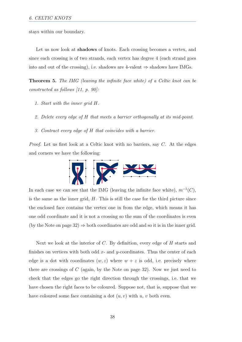
Proof. Let us first look at a Celtic knot with no barriers, say C. At the edges

and corners we have the following:

In each case we can see that the IMG (leaving the infinite face white), m−1(C),

is the same as the inner grid, H. This is still the case for the third picture since

the enclosed face contains the vertex one in from the edge, which means it has

one odd coordinate and it is not a crossing so the sum of the coordinates is even

(by the Note on page 32)⇒ both coordinates are odd and so it is in the inner grid.

Next we look at the interior of C. By definition, every edge of H starts and

finishes on vertices with both odd x- and y-coordinates. Thus the center of each

edge is a dot with coordinates (w, z) where w + z is odd, i.e. precisely where

there are crossings of C (again, by the Note on page 32). Now we just need to

check that the edges go the right direction through the crossings, i.e. that we

have chosen the right faces to be coloured. Suppose not, that is, suppose that we

have coloured some face containing a dot (u, v) with u, v both even.

38

6.3. Celtic Knots vs. Alternating Knots

Then as long as we pass through crossings, we keep meeting other coloured

faces. In particular, if we move directly Southward we keep passing through

crossings to faces containing dots (u, v − 2), (u, v − 4), . . . until we get to (u, 2).

But either (u − 1, 1) or (u + 1, 1) are already coloured as in our picture before,

and neighbouring (u, 2) so we have a contradiction. We find that there are no

faces coloured which contain a dot (u, v) with u, v both even, and so the other

faces are coloured in the process of constructing m−1(C)⇒ H = m−1(C).

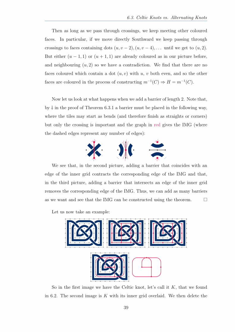
Now let us look at what happens when we add a barrier of length 2. Note that,

by†

in the proof of Theorem 6.3.1 a barrier must be placed in the following way,

where the tiles may start as bends (and therefore finish as straights or corners)

but only the crossing is important and the graph in red gives the IMG (where

the dashed edges represent any number of edges):

We see that, in the second picture, adding a barrier that coincides with an

edge of the inner grid contracts the corresponding edge of the IMG and that,

in the third picture, adding a barrier that intersects an edge of the inner grid

removes the corresponding edge of the IMG. Thus, we can add as many barriers

as we want and see that the IMG can be constructed using the theorem.

Let us now take an example:

So in the first image we have the Celtic knot, let’s call it K, that we found

in 6.2. The second image is K with its inner grid overlaid. We then delete the

39

6. CELTIC KNOTS

edges of the inner grid which orthogonally intersect barriers of K. This gives us

the third image. Next we contract the edges of the inner grid which coincide with

barriers of K. Removing the Celtic knot K from the background, we are left with

one of the two IMGs of the shadow s(K). We should note that since we are only

looking at Celtic knots and therefore alternating knots, s(K) can only be the

shadow of 1 or 2 non-equivalent knots. If we replace one vertex with a crossing,

all of the other crossings follow alternately. With the first vertex we have a choice

of an under- or over-crossing and so there are two possible knots that the shadow

defines. However, if K is amphichiral these two knots are equivalent anyway.

We are going to try to create a Celtic knot representation of some knot K

by precisely inverting the steps above. We will start by using the IMG of the

shadow of the knot, m−1(s(K)). Now, m−1(s(K)) may have vertices of any

degree. However, as we can see in the previous example, if we split a vertex

and replace the new edge with a barrier (moving from the fourth image to the

third), the medial graph remains the same. Intuitively this may seem to work,

but we need to be careful with this reuse of the word barrier. We have not yet

reached a grid environment, and so our definition of a barrier does not hold. Let

us therefore redefine it, in the context of an inverse medial graph.

Definition. A barrier b in a graph G is an edge with the following properties:

• Another edge cannot cross (under or over) b.

• b cannot be subdivided, i.e. a new vertex cannot be placed on b.

• If edges u and v are incident at either of the vertices that b is incident at,

then we say u and v share a vertex.

We draw a barrier as a dashed edge to distinguish it from the other edges.

When creating m(G) we can think of b and its end vertices as one ‘long vertex’,

since a barrier’s properties make it act like a vertex for this operation. The

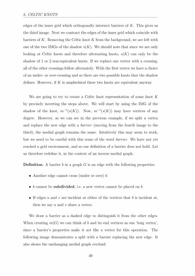
following image demonstrates a split with a barrier replacing the new edge. It

also shows the unchanging medial graph overlaid:

40

6.3. Celtic Knots vs. Alternating Knots

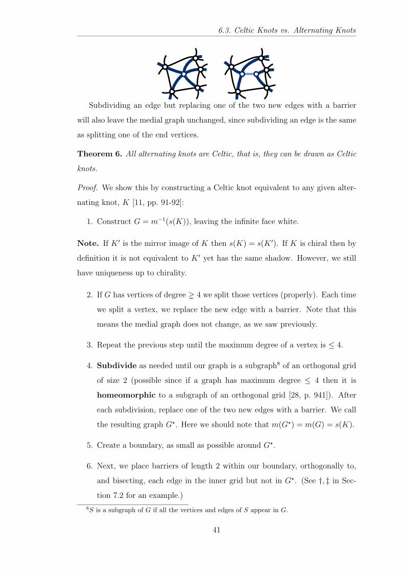
Subdividing an edge but replacing one of the two new edges with a barrier

will also leave the medial graph unchanged, since subdividing an edge is the same

as splitting one of the end vertices.

Theorem 6. All alternating knots are Celtic, that is, they can be drawn as Celtic

knots.

Proof. We show this by constructing a Celtic knot equivalent to any given alter-

nating knot, K [11, pp. 91-92]:

1. Construct G = m−1(s(K)), leaving the infinite face white.

Note. If K ′ is the mirror image of K then s(K) = s(K ′). If K is chiral then by

definition it is not equivalent to K ′ yet has the same shadow. However, we still

have uniqueness up to chirality.

2. If G has vertices of degree 4 we split those vertices (properly). Each time

we split a vertex, we replace the new edge with a barrier. Note that this

means the medial graph does not change, as we saw previously.

3. Repeat the previous step until the maximum degree of a vertex is ≤ 4.

4. Subdivide as needed until our graph is a subgraph8 of an orthogonal grid

of size 2 (possible since if a graph has maximum degree ≤ 4 then it is

homeomorphic to a subgraph of an orthogonal grid [28, p. 941]). After

each subdivision, replace one of the two new edges with a barrier. We call

the resulting graph G?. Here we should note that m(G?) = m(G) = s(K).

5. Create a boundary, as small as possible around G?.

6. Next, we place barriers of length 2 within our boundary, orthogonally to,

and bisecting, each edge in the inner grid but not in G?. (See †, ‡ in Sec-

tion 7.2 for an example.)

8S is a subgraph of G if all the vertices and edges of S appear in G.

41

6. CELTIC KNOTS

7. Remove G?, leaving behind its barriers and the new barriers.

8. Construct the knot that this set of barriers uniquely defines. (As shown in

Section 6.2.)

Once this is done, we have a Celtic knot C. Step 6 ensures the rest of the

algorithm constructs our knot by Theorem 5, since we have inverted both the

second and third steps of the theorem. Thus s(C) = m(G?) = m(G) = s(K).

That is, up to chirality, C is equivalent to K.

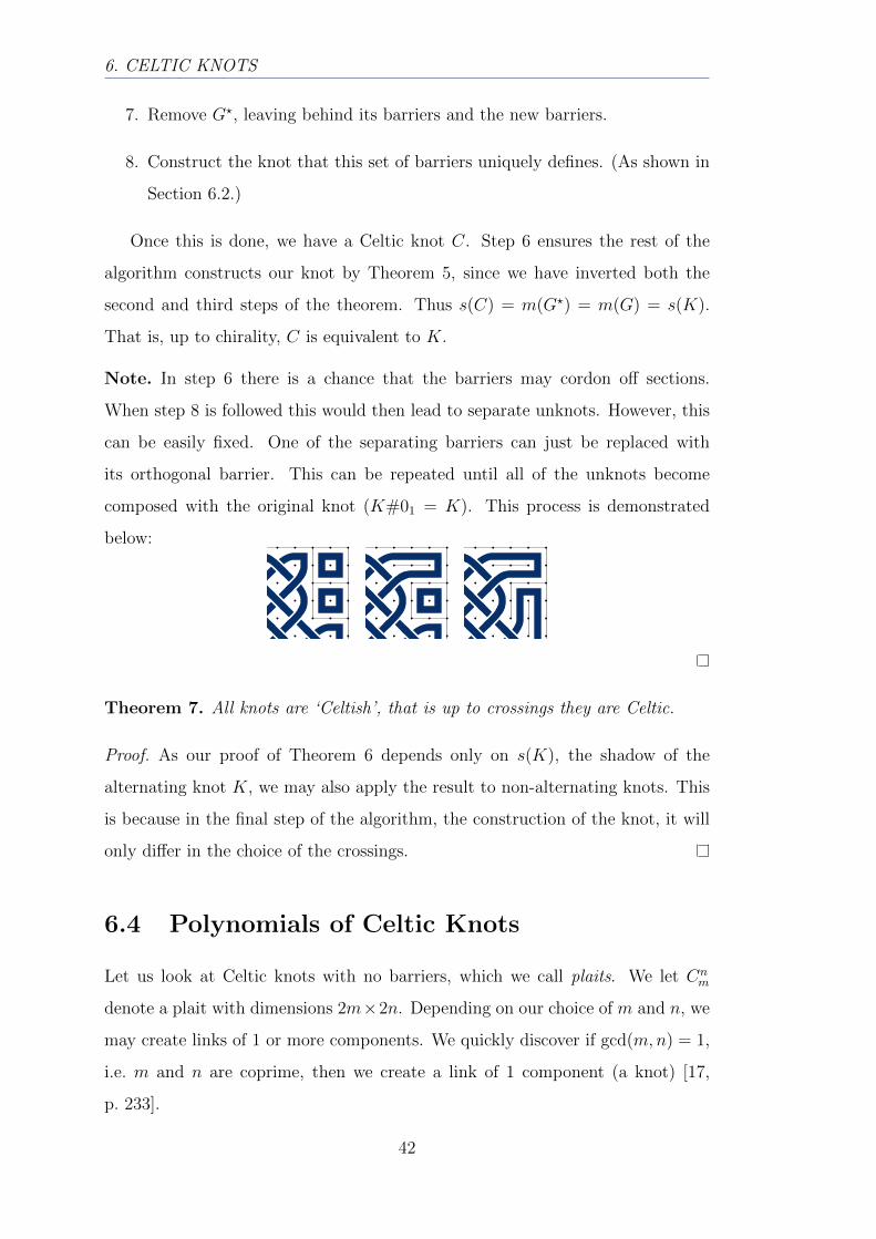
Note. In step 6 there is a chance that the barriers may cordon off sections.

When step 8 is followed this would then lead to separate unknots. However, this

can be easily fixed. One of the separating barriers can just be replaced with

its orthogonal barrier. This can be repeated until all of the unknots become

composed with the original knot (K#01 = K). This process is demonstrated

below:

Theorem 7. All knots are ‘Celtish’, that is up to crossings they are Celtic.

Proof. As our proof of Theorem 6 depends only on s(K), the shadow of the

alternating knot K, we may also apply the result to non-alternating knots. This

is because in the final step of the algorithm, the construction of the knot, it will

only differ in the choice of the crossings.

6.4 Polynomials of Celtic Knots

Let us look at Celtic knots with no barriers, which we call plaits. We let Cnm

denote a plait with dimensions 2m×2n. Depending on our choice of m and n, we

may create links of 1 or more components. We quickly discover if gcd(m,n) = 1,

i.e. m and n are coprime, then we create a link of 1 component (a knot) [17,

p. 233].

42

6.4. Polynomials of Celtic Knots

Theorem 8. If gcd(m,n) = k then the plait Cnm has exactly k components.

Proof. Let us replace bends and corners with diagonal tiles (ensuring that these

would fit our rules if we were to ignore barriers). We must still have the same

number of components, but now, walking along any tile’s strand we move ±1

both horizontally and vertically. Then to walk from one tile, say (x, y), along

its entire component and get back to (x, y), we must make 4am horizontal steps

(to the end and back a times) and 4bn vertical steps (to the top and bottom b

times) for some a, b ∈ N. Since every tile is diagonal, we must take as many

vertical as horizontal steps, so 4am = 4bn ⇒ am = bn. We want to know the

least number of steps in order to return, that is we want to find the a and b such

that am = bn = lcm(m,n). We note:

lcm(m,n) =mn

gcd(m,n)⇒ a =

n

gcd(m,n)and b =

m

gcd(m,n)

Since a is the number of times we crossed to the end and back, it must be the

number of times we turned around at, and hit, the vertical axis. This happens

at (0, 1), (0, 3), . . . , (0, 2n − 1) i.e. at n locations. (x, y) could have been on

any component, so every component must meet the vertical axis exactly a times.

Thus, the number of components is na

= gcd(m,n).

Theorem 9. C2m has Conway polynomial

(−z +√

1 + z2)m − (−z −√

1 + z2)m

2√

1 + z2.

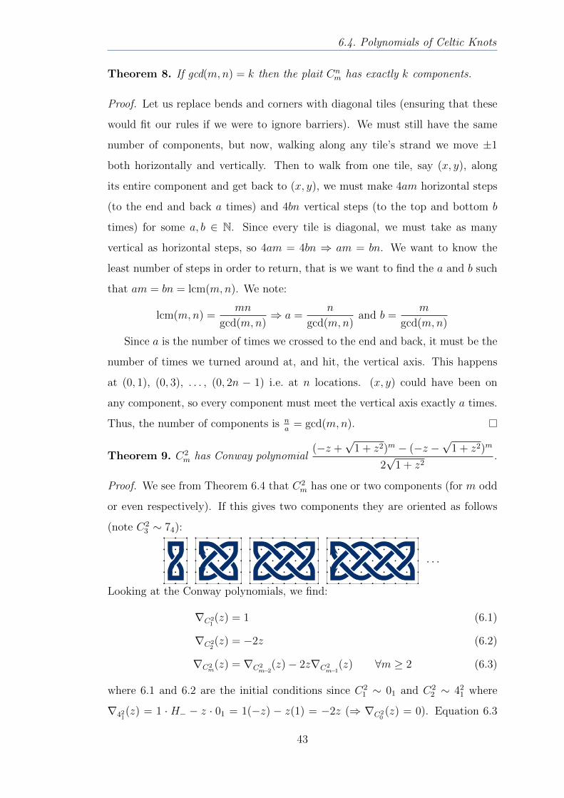
Proof. We see from Theorem 6.4 that C2m has one or two components (for m odd

or even respectively). If this gives two components they are oriented as follows

(note C23 ∼ 74):

· · ·

Looking at the Conway polynomials, we find:

∇C21(z) = 1 (6.1)

∇C22(z) = −2z (6.2)

∇C2m

(z) = ∇C2m−2

(z)− 2z∇C2m−1

(z) ∀m ≥ 2 (6.3)

where 6.1 and 6.2 are the initial conditions since C21 ∼ 01 and C2

2 ∼ 421 where

∇421(z) = 1 · H− − z · 01 = 1(−z) − z(1) = −2z (⇒ ∇C2

0(z) = 0). Equation 6.3

43

6. CELTIC KNOTS

comes from the following skein tree (where H = 2(m−2), • = 2(m−1), � = 2m:

Now that we have a recurrence relation and initial conditions we can find the

solution for any m. First of all we find the roots of the characteristic equation:

c(r) = r2 + 2zr − 1

(r + z)2 − z2 − 1 = 0

r = −z ±√

1 + z2.

Then the solution to the recurrence takes the form:

∇C2m

(z) = α1(−z +√

1 + z2)m + α2(−z −√

1 + z2)m

m = 0⇒ α1 = −α2

m = 1⇒ 1 = α1(−z +√

1 + z2)− α1(−z −√

1 + z2)

= 2α1

√1 + z2

α1 =1

2√

1 + z2, α2 =

−1

2√

1 + z2

∇C2m

(z) =(−z +

√1 + z2)m − (−z −

√1 + z2)m

2√

1 + z2.

⇒ 74 ∼ C23 has Conway polynomial given by:

∇74(z) =(−z +

√1 + z2)3 − (−z −

√1 + z2)3

2√

1 + z2

=8z2√

1 + z2 + 2√

1 + z2

2√

1 + z2

= 1 + 4z2.

44

6.5. Celtic Invariants

6.5 Celtic Invariants

Now that we have examined how the Conway polynomial invariant relates to

Celtic knots, we can investigate other invariants specific to the rules that we have

defined for Celtic (and Celtish) knots:

Minimum Area, α. For a knot, K, the minimum area is defined to be the

minimum number of tiles that any Celtish knot, K ′, can be drawn on, for all

K ′ ∼ K. Clearly if our boundary dimensions are 2m× 2n then the area is 4mn.

Minimum Number of Barriers, β. The minimum b, where b is the number of

barriers of length 2, that any Celtish knot, K ′, can be drawn with, for all K ′ ∼ K.

Minimum Dimension, δ. The minimum dimension for a knot, K, is the small-

est width (or height) that any Celtish knot, K ′, can be drawn with, for allK ′ ∼ K.

For all non-trivial knots, the minimum dimension ≥ 4. This is because if we have

a knot with boundary dimensions 2m × 2n and either m or n = 1, say n = 1,

then with n− 1− b twists (i.e. Type I moves) we have the unknot.

Minimum Perimeter, π. Defined as for area and barriers.

The following relations are useful to derive lower bounds for the above invariants:

Theorem 10. If c is the number of crossings in the Celtish knot we have that

c+ b = 2mn−m− n. Also, 4mn ≥ 2b+ 2c+ 8 and 4mn ≥ 2c+ 8.

Proof. For every dot inside our boundary with coordinates (x, y), where x+ y is

odd, there is a crossing or a barrier of length 2 by the Note on page 32. The Note

also shows that barriers and crossings cannot be anywhere else.

Now, for the m odd columns (at y = 1, . . . , 2m−1) we need even rows (so that

x+ y is odd as above) which are at x = 2, . . . , 2n−2 implying that we have n−1

even rows. For the m−1 even columns (at y = 2, . . . , 2m−2) we need odd rows (so

45

6. CELTIC KNOTS

that x+y is odd) which are at x = 1, . . . , 2n−1 implying that we have n odd rows.

Thus the number of crossings and barriers is c+ b = m(n− 1) + n(m− 1) =

2mn−m− n.

We find if b is minimised and the boundary dimensions, 2m×2n, are minimised

then the minimum area is 4mn = 2b + 2c + 2m + 2n. Now, since the minimum

dimension is ≥ 4 we have m,n ≥ 2 ⇒ 4mn ≥ 2b + 2c + 8 and b ≥ 0 ⇒ 4mn ≥

2c+ 8.

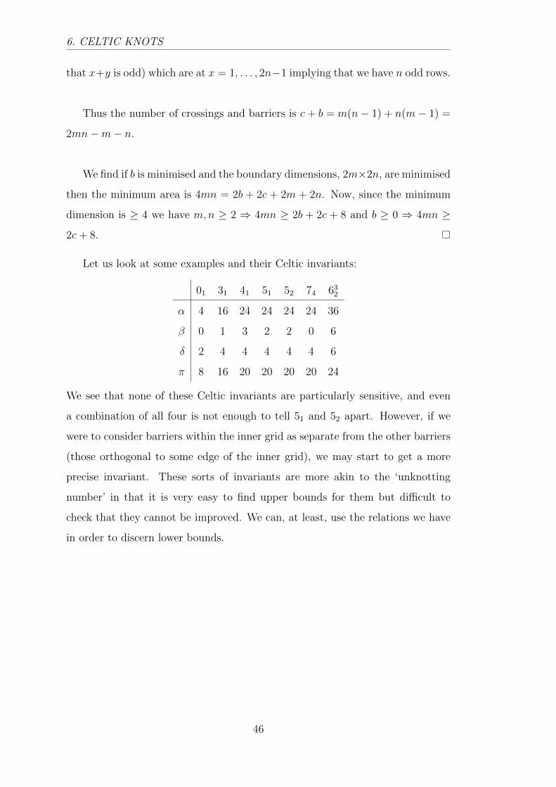
Let us look at some examples and their Celtic invariants:

01 31 41 51 52 74 632

α 4 16 24 24 24 24 36

β 0 1 3 2 2 0 6

δ 2 4 4 4 4 4 6

π 8 16 20 20 20 20 24

We see that none of these Celtic invariants are particularly sensitive, and even

a combination of all four is not enough to tell 51 and 52 apart. However, if we

were to consider barriers within the inner grid as separate from the other barriers

(those orthogonal to some edge of the inner grid), we may start to get a more

precise invariant. These sorts of invariants are more akin to the ‘unknotting

number’ in that it is very easy to find upper bounds for them but difficult to

check that they cannot be improved. We can, at least, use the relations we have

in order to discern lower bounds.

46

Chapter 7

Brunnian Links

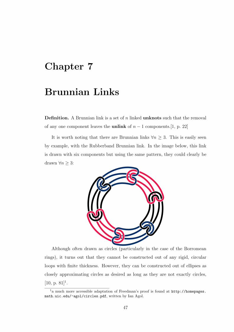
Definition. A Brunnian link is a set of n linked unknots such that the removal

of any one component leaves the unlink of n− 1 components.[1, p. 22]

It is worth noting that there are Brunnian links ∀n ≥ 3. This is easily seen

by example, with the Rubberband Brunnian link. In the image below, this link

is drawn with six components but using the same pattern, they could clearly be

drawn ∀n ≥ 3:

Although often drawn as circles (particularly in the case of the Borromean

rings), it turns out that they cannot be constructed out of any rigid, circular

loops with finite thickness. However, they can be constructed out of ellipses as

closely approximating circles as desired as long as they are not exactly circles,

[10, p. 81]1.

1a much more accessible adaptation of Freedman’s proof is found at http://homepages.

math.uic.edu/~agol/circles.pdf, written by Ian Agol.

47

7. BRUNNIAN LINKS

7.1 n = 3: Borromean Rings, 632

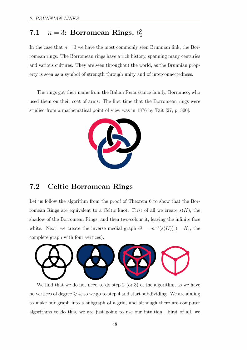
In the case that n = 3 we have the most commonly seen Brunnian link, the Bor-

romean rings. The Borromean rings have a rich history, spanning many centuries

and various cultures. They are seen throughout the world, as the Brunnian prop-

erty is seen as a symbol of strength through unity and of interconnectedness.

The rings got their name from the Italian Renaissance family, Borromeo, who

used them on their coat of arms. The first time that the Borromean rings were

studied from a mathematical point of view was in 1876 by Tait [27, p. 300].

7.2 Celtic Borromean Rings

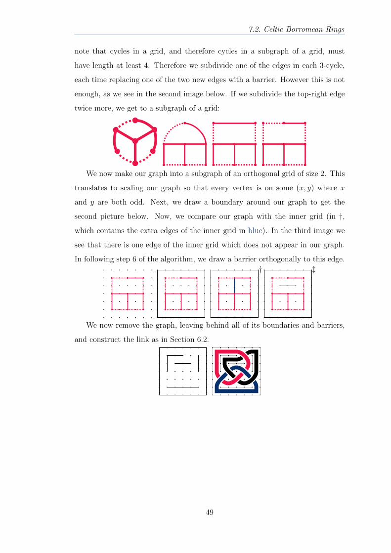
Let us follow the algorithm from the proof of Theorem 6 to show that the Bor-

romean Rings are equivalent to a Celtic knot. First of all we create s(K), the

shadow of the Borromean Rings, and then two-colour it, leaving the infinite face

white. Next, we create the inverse medial graph G = m−1(s(K)) (= K4, the

complete graph with four vertices).

We find that we do not need to do step 2 (or 3) of the algorithm, as we have

no vertices of degree 4, so we go to step 4 and start subdividing. We are aiming

to make our graph into a subgraph of a grid, and although there are computer

algorithms to do this, we are just going to use our intuition. First of all, we

48

7.2. Celtic Borromean Rings

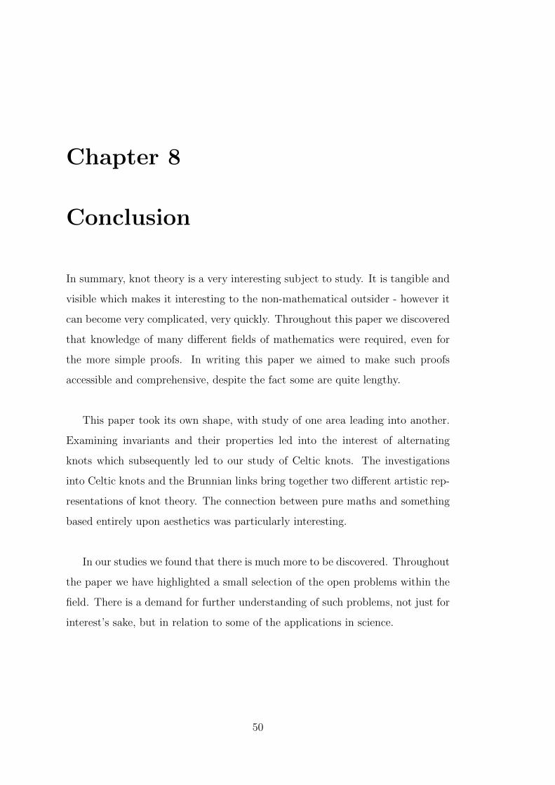
note that cycles in a grid, and therefore cycles in a subgraph of a grid, must

have length at least 4. Therefore we subdivide one of the edges in each 3-cycle,

each time replacing one of the two new edges with a barrier. However this is not

enough, as we see in the second image below. If we subdivide the top-right edge

twice more, we get to a subgraph of a grid:

We now make our graph into a subgraph of an orthogonal grid of size 2. This

translates to scaling our graph so that every vertex is on some (x, y) where x

and y are both odd. Next, we draw a boundary around our graph to get the

second picture below. Now, we compare our graph with the inner grid (in †,

which contains the extra edges of the inner grid in blue). In the third image we

see that there is one edge of the inner grid which does not appear in our graph.

In following step 6 of the algorithm, we draw a barrier orthogonally to this edge.

† ‡

We now remove the graph, leaving behind all of its boundaries and barriers,

and construct the link as in Section 6.2.

49

Chapter 8

Conclusion

In summary, knot theory is a very interesting subject to study. It is tangible and

visible which makes it interesting to the non-mathematical outsider - however it

can become very complicated, very quickly. Throughout this paper we discovered

that knowledge of many different fields of mathematics were required, even for

the more simple proofs. In writing this paper we aimed to make such proofs

accessible and comprehensive, despite the fact some are quite lengthy.

This paper took its own shape, with study of one area leading into another.

Examining invariants and their properties led into the interest of alternating

knots which subsequently led to our study of Celtic knots. The investigations

into Celtic knots and the Brunnian links bring together two different artistic rep-

resentations of knot theory. The connection between pure maths and something

based entirely upon aesthetics was particularly interesting.

In our studies we found that there is much more to be discovered. Throughout

the paper we have highlighted a small selection of the open problems within the

field. There is a demand for further understanding of such problems, not just for

interest’s sake, but in relation to some of the applications in science.

50

Glossary

Ambient Isotopy: Two knots are ambient isotopic if there exists a deformation

of one knot, without breaking it or allowing it to intersect itself, into the

other [1, p. 12].

Chirality: A knot is amphichiral if it is equivalent to its mirror image [1, p. 175],

e.g. the figure eight knot, see 4.1.2. Otherwise, it is a chiral knot, e.g. the

trefoil knot, see 4.1.1.

Crossing Number: n is the crossing number of a knot, K, i.e. c(K) = n, if

there exists a link diagram of K with n crossings and no link diagrams of

K with fewer than n crossings [1, p. 3].

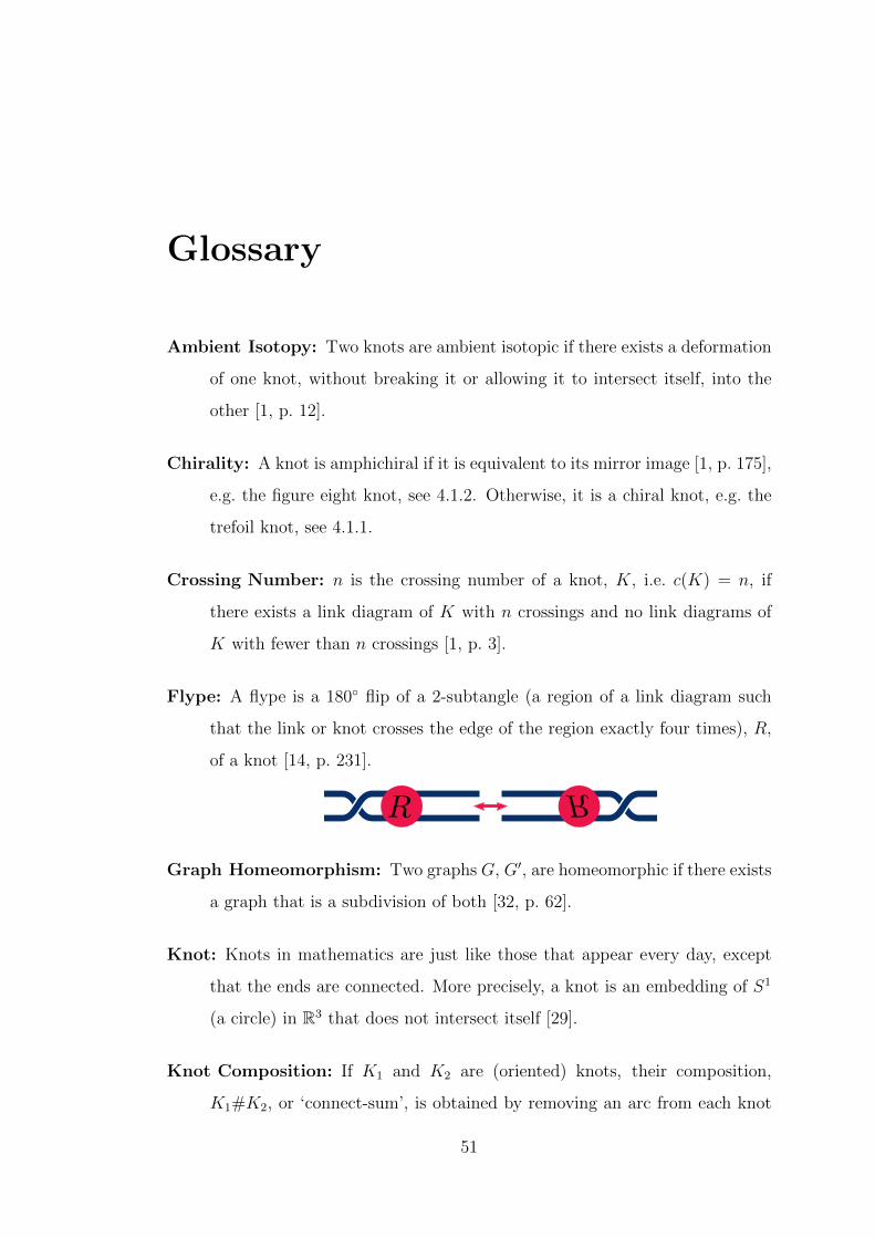
Flype: A flype is a 180◦ flip of a 2-subtangle (a region of a link diagram such

that the link or knot crosses the edge of the region exactly four times), R,

of a knot [14, p. 231].

Graph Homeomorphism: Two graphs G, G′, are homeomorphic if there exists

a graph that is a subdivision of both [32, p. 62].

Knot: Knots in mathematics are just like those that appear every day, except

that the ends are connected. More precisely, a knot is an embedding of S1

(a circle) in R3 that does not intersect itself [29].

Knot Composition: If K1 and K2 are (oriented) knots, their composition,

K1#K2, or ‘connect-sum’, is obtained by removing an arc from each knot

51

GLOSSARY

and splicing the ends to achieve a single component (ensuring the orienta-

tion is consistent on the new knot) [1, pp. 7-11]. We then call K1 and K2

the ‘factor knots’.

Knot Equivalence: Two knots K,K ′are equivalent if one is an ambient isotopy

of the other. We write K ∼ K ′. Reidemeister’s Theorem states that two

link diagrams (and therefore any two links) are equivalent if and only if

they are connected by a sequence of Reidemeister moves [22].

Knot Invariant: A knot invariant is some measure of a knot, K, that is fixed

for all knots equivalent to K [1, p. 21].

Link: A link is a set of knots that do not intersect but may be linked together (if

not, we say the link is splittable). Thus a knot is a link of one component

[1, p. 17].

Link Diagram: A link diagram of a link is a projection of the link onto a plane.

By selecting an appropriate direction of projection one can arrange it so

that the projection is one-to-one except at the transverse (or ‘single point’)

intersections of two strands, called crossings. The strands are then identified

by creating a break in the under-strand [30]. (See (4.1.1) for an example.)

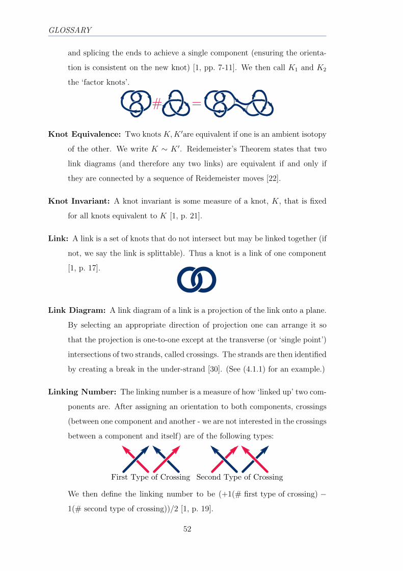
Linking Number: The linking number is a measure of how ‘linked up’ two com-

ponents are. After assigning an orientation to both components, crossings

(between one component and another - we are not interested in the crossings

between a component and itself) are of the following types:

We then define the linking number to be (+1(# first type of crossing) −

1(# second type of crossing))/2 [1, p. 19].

52

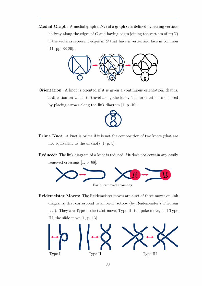
Medial Graph: A medial graph m(G) of a graph G is defined by having vertices

halfway along the edges of G and having edges joining the vertices of m(G)

if the vertices represent edges in G that have a vertex and face in common

[11, pp. 88-89].

Orientation: A knot is oriented if it is given a continuous orientation, that is,

a direction on which to travel along the knot. The orientation is denoted

by placing arrows along the link diagram [1, p. 10].

Prime Knot: A knot is prime if it is not the composition of two knots (that are

not equivalent to the unknot) [1, p. 9].

Reduced: The link diagram of a knot is reduced if it does not contain any easily

removed crossings [1, p. 68].

Reidemeister Moves: The Reidemeister moves are a set of three moves on link

diagrams, that correspond to ambient isotopy (by Reidemeister’s Theorem

[22]). They are Type I, the twist move, Type II, the poke move, and Type

III, the slide move [1, p. 13].

53

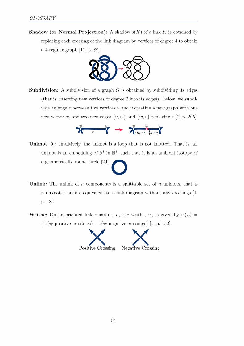
GLOSSARY

Shadow (or Normal Projection): A shadow s(K) of a link K is obtained by

replacing each crossing of the link diagram by vertices of degree 4 to obtain

a 4-regular graph [11, p. 89].

Subdivision: A subdivision of a graph G is obtained by subdividing its edges

(that is, inserting new vertices of degree 2 into its edges). Below, we subdi-

vide an edge e between two vertices u and v creating a new graph with one

new vertex w, and two new edges {u,w} and {w, v} replacing e [2, p. 205].

Unknot, 01: Intuitively, the unknot is a loop that is not knotted. That is, an

unknot is an embedding of S1 in R3, such that it is an ambient isotopy of

a geometrically round circle [29].

Unlink: The unlink of n components is a splittable set of n unknots, that is

n unknots that are equivalent to a link diagram without any crossings [1,

p. 18].

Writhe: On an oriented link diagram, L, the writhe, w, is given by w(L) =

+1(# positive crossings)− 1(# negative crossings) [1, p. 152].

54

Bibliography

[1] Adams, C.C. (2004). The Knot Book: An Elementary Introduction to the

Mathematical Theory of Knots, American Mathematical Society.

[2] Agnarsson, G. & Greenlaw, R. (2007). Graph Theory: Modeling, Applica-

tions, and Algorithms, Pearson/Prentice Hall.

[3] Alexander, J.W. (1928). Topological Invariants of Knots and Links. In Trans-

actions of the American Mathematical Society, Vol. 30 (2), pp. 275-306.

[4] Bollobas, B. (1998). Modern Graph Theory, Springer.

[5] Cha, J.C. & Livingston, C. KnotInfo: Table of Knot Invariants. http://

www.indiana.edu/~knotinfo (as of 15 October 2011)

[6] Conway, J.H. (1969). An enumeration of knots and links, and some of their

algebraic properties. In Computational Problems in Abstract Algebra (Ed. J.

Leech), Pergamon Press, pp. 329-358.

[7] Crowell, R.H. (1959). Genus of alternating link types. In The Annals of

Mathematics Ser. 2 Vol. 69 (2), pp. 258-275.

[8] Epple, M. (1998). Topology, Matter, and Space, I: Topological Notions in

19th-Century Natural Philosophy. In Archive for History of Exact Sciences

Vol. 52 (4), Springer, pp. 297-392.

[9] Flapan, E. (2000). When Topology Meets Chemistry: A Topological Look at

Molecular Chirality, Cambridge University Press.

[10] Freedman, M.H. & Skora, R. (1987) Strange Actions of Groups on Spheres.

In J. Differential Geometry Vol. 25, pp. 75-98.

55

BIBLIOGRAPHY

[11] Gross, J.L. & Tucker, T.W. (2011) A Celtic Framework for Knots and Links.

In Discrete & Computational Geometry Vol. 46 (1), pp. 86-99.

[12] Hoste, J., Thistlethwaite, M. & Weeks, J. (1998). The first 1,701,936 knots.

In The Mathematical Intelligencer Vol. 20 (4), pp. 33-48.

[13] Jones, V.F.R. (1985). A Polynomial Invariant for Knots via von Neumann

Algebras. In Bull. 12 (1), American Mathematical Society, pp. 103-111.

[14] Kauffman, L.H. & Lambropoulou, S. (2003). Classifying and applying ra-

tional knots and rational tangles. In Physical Knots: Knotting, Linking and

Folding Geometric Objects in R3 (Eds. J.A. Calvo, K.C. Millett & E.J. Raw-

don), American Mathematical Society, pp. 223-260.

[15] Kinoshita, S. & Terasaka, H. (1957). On unions of knots. In Osaka Math. J.

Vol. 9, pp. 131-153.

[16] Kirby, R. (1995). Problems in Low-Dimensional Topology. ftp://math.

berkeley.edu/pub/Preprints/Rob_Kirby/Problems/problems.ps.gz (as

of 10 November 2012)

[17] Meehan, A. (2007). The Celtic Design Book, Thames & Hudson.

[18] Menasco, W. & Thistlethwaite, M. (1993). The classification of alternating

links. In Annals of Mathematics Vol. 138, pp. 113-171.

[19] Menasco, W. & Thistlethwaite, M. (2005). Handbook of Knot Theory, Else-

vier.

[20] Murasugi, K. (1958). On the Alexander Polynomial of the Alternating Knot.

In Osaka Math. J. Vol. 10, pp. 181-189.

[21] Murasugi, K. (1987). Jones Polynomial and Classical Conjectures in Knot

Theory. In Topology Vol. 26 (2), pp. 187-194.

[22] Murasugi, K. (2008). Knot Theory and its Applications, Birkhauser Boston.

[23] Nash, C. (2008). Topology and Physics - A Historical Essay. In History of

Topology (Ed. I.M. James), North-Holland, pp. 359-416.

56

[24] Przytycki, J.H. (1992). History of the Knot Theory From Vandermonde to

Jones. In Aportaciones Matematicas Comunicaciones Vol. 11, pp. 173-185.

[25] Silver, D.S. (2006). Knot Theory’s Odd Origins. In American Scientist

Vol. 94 (2), pp. 158-165.

[26] Sossinsky, A. (2002). Knots: Mathematics with a Twist, Harvard University

Press.

[27] Tait, P.G. (1876-7). On Knots. In Scientific Papers Vol. 1, Cambridge Uni-

versity Press, pp. 273-348.

[28] Tamassia, R. (1999). Graph Drawing. In Handbook of Computational Geom-

etry (Eds. J.-R. Sack, J. Urrutia), Elsevier, pp. 937-971.

[29] Weisstein, E.W. “Knot.” From MathWorld–A Wolfram Web Resource.

http://mathworld.wolfram.com/Knot.html (as of 12 October 2011)

[30] Weisstein, E.W. “Link Diagram.” From MathWorld–A Wolfram Web Re-

source. http://mathworld.wolfram.com/LinkDiagram.html (as of 15 Oc-

tober 2011)

[31] Weisstein, E.W. “Trefoil Knot.” From MathWorld–A Wolfram Web Re-

source. http://mathworld.wolfram.com/TrefoilKnot.html (as of 18 Oc-

tober 2011)

[32] Wilson, R.J. (1996). Introduction to Graph Theory, Longman Group Ltd.

57