cebok module 3 parametric estimating - presentation · costing techniques 3. parametric estimating...
TRANSCRIPT
PT02 - Cost Estimating Relationships
ICEAA 2014 Professional Development & Training Workshop
1
© 2002-2010 ICEAA. All rights reserved.
v1.0
1
Parametric Estimating Handbook (4th ed.), ISPA, 2007.
PT 02 – Cost Estimating Relationships
Adapted from:
CEBOK Module 3 &
ISPA Parametric Estimating Handbook
“Parametric estimating is a technique that develops cost estimates based
upon the examination and validation of the relationships which exist
between a project's technical, programmatic, and cost characteristics as
well as the resources consumed during its development, manufacture,
maintenance, and/or modification.”
-Parametric Estimating Handbook
© 2002-2010 ICEAA. All rights reserved.
v1.0
2
Unit Index
Unit I – Cost Estimating
1. Cost Estimating Basics
2. Costing Techniques
3. Parametric Estimating
Unit II – Cost Analysis Techniques
Unit III – Analytical Methods
Unit IV – Specialized Costing
Unit V – Management Applications
PT02 - Cost Estimating Relationships
ICEAA 2014 Professional Development & Training Workshop
2
© 2002-2010 ICEAA. All rights reserved.
v1.0
3
Parametric Estimating Overview
• Key Ideas
– Cost Drivers (and “Cost
Passengers”)
– Inputs and Outputs
– Parametric Models
• Practical Applications
– CER Development
– Cost Response Curves (CRCs)
– Sensitivity Analysis
– Schedule or Weight Estimating
Relationships
• Analytical Constructs
– Linear equations
– Other functional forms
• Power, exponential, log,
polynomial
– Curve fitting
• Related Topics
– COTS Cost Models
– Manufacturing Cost
Estimating
– Software Cost Estimating
– Trade Studies
NEW!
3
11
12
16
© 2002-2010 ICEAA. All rights reserved.
v1.0
4
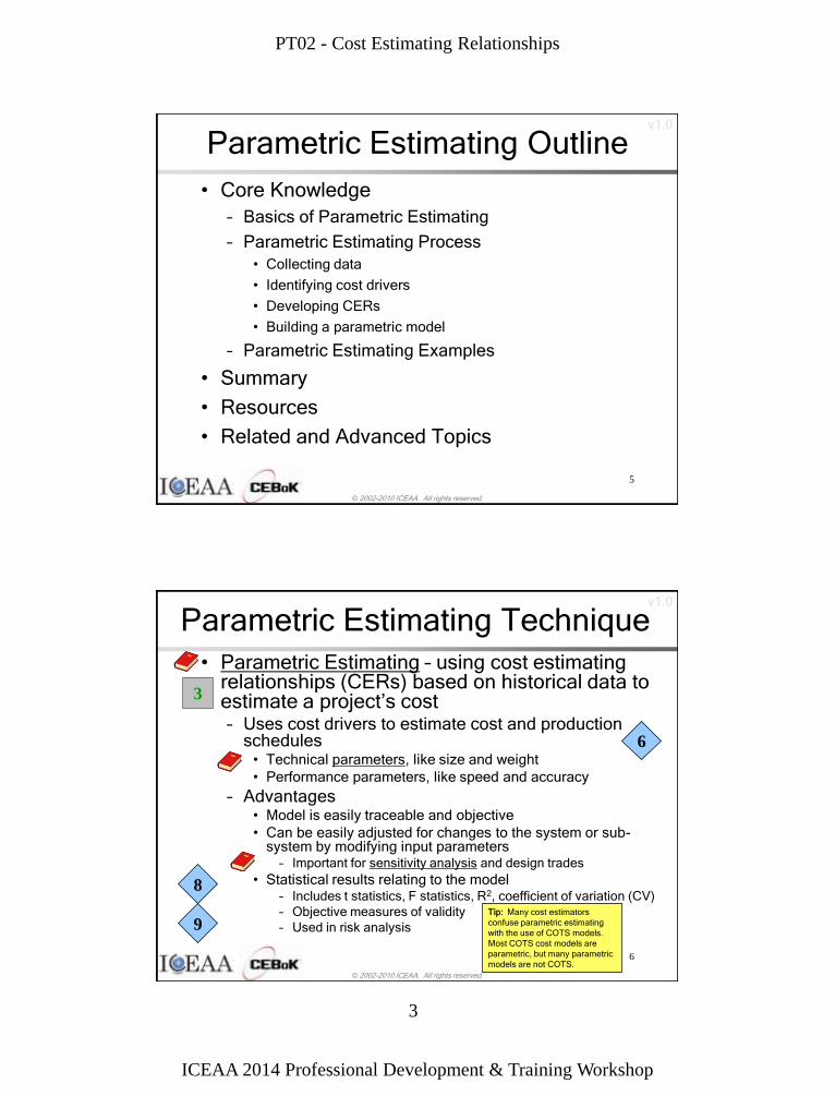
Parametric Estimating Within The
Cost Estimating Framework
Past Understanding your
historical data
Present Developing
estimating tools
Future Estimating the new
system
Historical costs
for similar
systems
Cost
Estimating
Relationships
Applying,
Validating, and
Updating CERs
NEW!
Site Activation
y = 26.491x + 82.756
R2 = 0.9098
$-
$200
$400
$600
$800
$1,000
$1,200
$1,400
0 10 20 30 40 50
Number of Workstations Installed
Co
st
($K
)
Site Activation
$-
$200
$400
$600
$800
$1,000
$1,200
$1,400
0 10 20 30 40 50
Number of Workstations Installed
Co
st
($K
)
Site Activation
y = 26.635x + 105.16
R2 = 0.9099
$-
$200
$400
$600
$800
$1,000
$1,200
$1,400
$1,600
0 10 20 30 40 50
Number of Workstations Installed
Co
st
($K
)
4
PT02 - Cost Estimating Relationships
ICEAA 2014 Professional Development & Training Workshop
3
© 2002-2010 ICEAA. All rights reserved.
v1.0
5
Parametric Estimating Outline
• Core Knowledge
– Basics of Parametric Estimating
– Parametric Estimating Process
• Collecting data
• Identifying cost drivers
• Developing CERs
• Building a parametric model
– Parametric Estimating Examples
• Summary
• Resources
• Related and Advanced Topics
© 2002-2010 ICEAA. All rights reserved.
v1.0
6
Parametric Estimating Technique
• Parametric Estimating – using cost estimating relationships (CERs) based on historical data to estimate a project’s cost – Uses cost drivers to estimate cost and production
schedules • Technical parameters, like size and weight
• Performance parameters, like speed and accuracy
– Advantages • Model is easily traceable and objective
• Can be easily adjusted for changes to the system or sub-system by modifying input parameters
– Important for sensitivity analysis and design trades
• Statistical results relating to the model – Includes t statistics, F statistics, R2, coefficient of variation (CV)
– Objective measures of validity
– Used in risk analysis
6
8
9
3
Tip: Many cost estimators
confuse parametric estimating
with the use of COTS models.
Most COTS cost models are
parametric, but many parametric
models are not COTS.
PT02 - Cost Estimating Relationships
ICEAA 2014 Professional Development & Training Workshop
4
© 2002-2010 ICEAA. All rights reserved.
v1.0
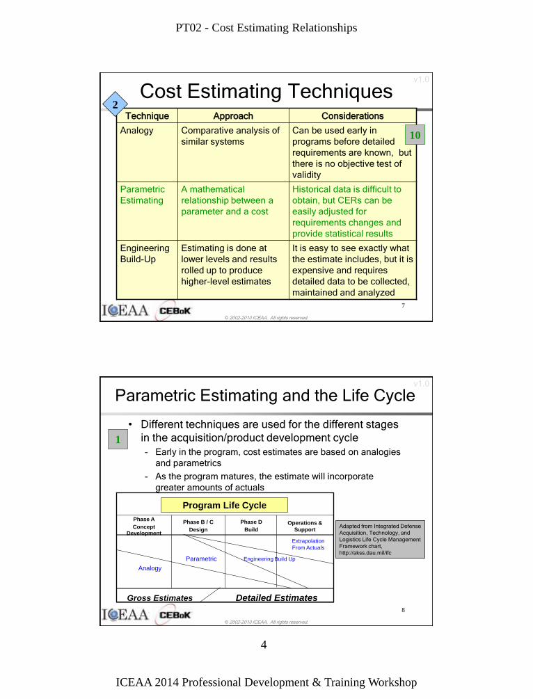
7
Technique Approach Considerations
Analogy Comparative analysis of
similar systems
Can be used early in
programs before detailed
requirements are known, but
there is no objective test of
validity
Parametric
Estimating
A mathematical
relationship between a
parameter and a cost
Historical data is difficult to
obtain, but CERs can be
easily adjusted for
requirements changes and
provide statistical results
Engineering
Build-Up
Estimating is done at
lower levels and results
rolled up to produce
higher-level estimates
It is easy to see exactly what
the estimate includes, but it is
expensive and requires
detailed data to be collected,
maintained and analyzed
Cost Estimating Techniques 2
10
© 2002-2010 ICEAA. All rights reserved.
v1.0
8
Parametric Estimating and the Life Cycle
• Different techniques are used for the different stages
in the acquisition/product development cycle
– Early in the program, cost estimates are based on analogies
and parametrics
– As the program matures, the estimate will incorporate
greater amounts of actuals
1
Adapted from Integrated Defense
Acquisition, Technology, and
Logistics Life Cycle Management
Framework chart,
http://akss.dau.mil/ifc
Program Life Cycle
Gross Estimates Detailed Estimates
Analogy
Parametric
Extrapolation
From Actuals
Engineering Build Up
Phase A
Concept Development
Phase B / C
Design
Phase D
Build
Operations &
Support
PT02 - Cost Estimating Relationships
ICEAA 2014 Professional Development & Training Workshop
5
© 2002-2010 ICEAA. All rights reserved.
v1.0
9
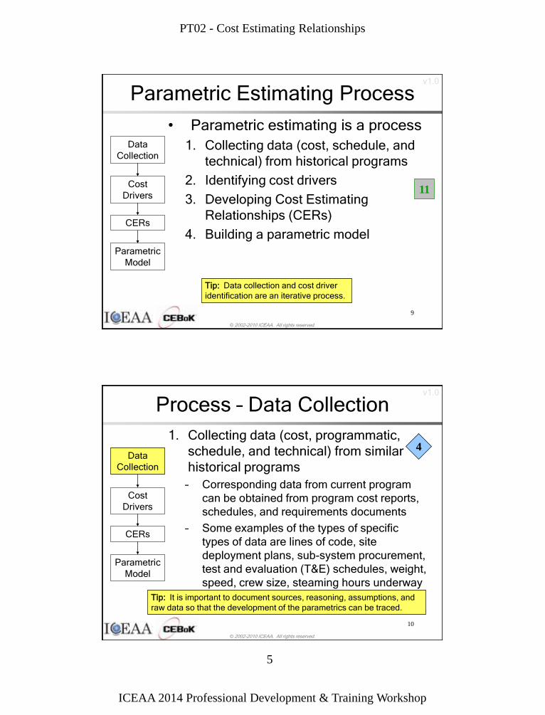
Parametric Estimating Process
• Parametric estimating is a process
1. Collecting data (cost, schedule, and
technical) from historical programs
2. Identifying cost drivers
3. Developing Cost Estimating
Relationships (CERs)
4. Building a parametric model
Cost
Drivers
CERs
Parametric
Model
Data
Collection
11
Tip: Data collection and cost driver
identification are an iterative process.
© 2002-2010 ICEAA. All rights reserved.
v1.0
10
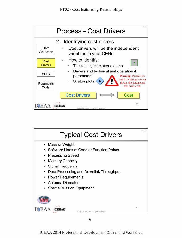
Process – Data Collection
1. Collecting data (cost, programmatic,
schedule, and technical) from similar
historical programs
– Corresponding data from current program
can be obtained from program cost reports,
schedules, and requirements documents
– Some examples of the types of specific
types of data are lines of code, site
deployment plans, sub-system procurement,
test and evaluation (T&E) schedules, weight,
speed, crew size, steaming hours underway
(SHU)
4
Tip: It is important to document sources, reasoning, assumptions, and
raw data so that the development of the parametrics can be traced.
Cost
Drivers
CERs
Parametric
Model
Data
Collection
PT02 - Cost Estimating Relationships
ICEAA 2014 Professional Development & Training Workshop
6
© 2002-2010 ICEAA. All rights reserved.
v1.0
11
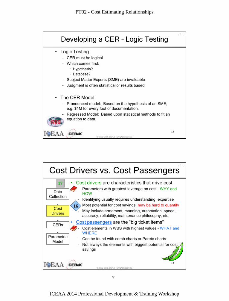
Process – Cost Drivers
2. Identifying cost drivers
– Cost drivers will be the independent
variables in your CERs
– How to identify:
• Talk to subject matter experts
• Understand technical and operational
parameters
• Scatter plots 6
Cost
Drivers
CERs
Parametric
Model
Data
Collection
Cost Cost Drivers
2
Warning: Parameters
that drive design are not
always the parameters
that drive cost.
© 2002-2010 ICEAA. All rights reserved.
v1.0
Typical Cost Drivers
• Mass or Weight
• Software Lines of Code or Function Points
• Processing Speed
• Memory Capacity
• Signal Frequency
• Data-Processing and Downlink Throughput
• Power Requirements
• Antenna Diameter
• Special Mission Equipment
12
PT02 - Cost Estimating Relationships
ICEAA 2014 Professional Development & Training Workshop
7
© 2002-2010 ICEAA. All rights reserved.
v1.0
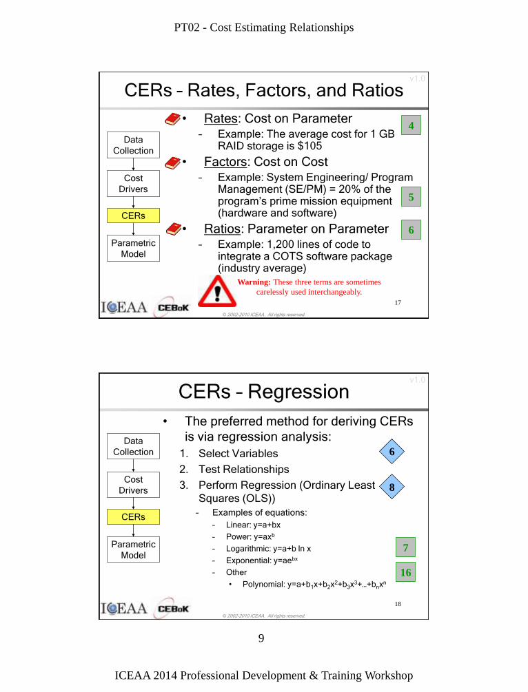
Developing a CER – Logic Testing
• Logic Testing
– CER must be logical
– Which comes first:
• Hypothesis?
• Database?
– Subject Matter Experts (SME) are invaluable
– Judgment is often statistical or results based
• The CER Model
– Pronounced model: Based on the hypothesis of an SME;
e.g. $1M for every foot of documentation.
– Regressed Model: Based upon statistical methods to fit an
equation to data.
13
© 2002-2010 ICEAA. All rights reserved.
v1.0
14
Cost Drivers vs. Cost Passengers
• Cost drivers are characteristics that drive cost
– Parameters with greatest leverage on cost – WHY and
HOW
– Identifying usually requires understanding, expertise
– Most potential for cost savings, may be hard to quantify
– May include armament, manning, automation, speed,
accuracy, reliability, maintenance philosophy, etc.
• Cost passengers are the “big ticket items”
– Cost elements in WBS with highest values – WHAT and
WHERE
– Can be found with comb charts or Pareto charts
– Not always the elements with biggest potential for cost
savings
Cost
Drivers
CERs
Parametric
Model
Data
Collection
16
17

PT02 - Cost Estimating Relationships
ICEAA 2014 Professional Development & Training Workshop
8
© 2002-2010 ICEAA. All rights reserved.
v1.0
15
Process – CERs
3. Developing Cost Estimating
Relationships (CERs)
– After the available historical and industry data
are collected for the system, the cost analyst
then analyzes “relationships” within the data y = 0.3075x + 66.337
R2 = 0.4705
70.00
80.00
90.00
100.00
110.00
120.00
130.00
40.00 90.00 140.00
Variable 1
Co
st
6
Cost
Drivers
CERs
Parametric
Model
Data
Collection
© 2002-2010 ICEAA. All rights reserved.
v1.0
Continuum of CER Complexity
16
Simple Relationship (Ratio)
Complex Relationships (Multi-variable equations)
Models (Many equations)
Increasing Complexity of Method/Relationship
PT02 - Cost Estimating Relationships
ICEAA 2014 Professional Development & Training Workshop
9
© 2002-2010 ICEAA. All rights reserved.
v1.0
17
CERs – Rates, Factors, and Ratios
• Rates: Cost on Parameter – Example: The average cost for 1 GB
RAID storage is $105
• Factors: Cost on Cost – Example: System Engineering/ Program
Management (SE/PM) = 20% of the program’s prime mission equipment (hardware and software)
• Ratios: Parameter on Parameter – Example: 1,200 lines of code to
integrate a COTS software package (industry average)
Cost
Drivers
CERs
Parametric
Model
Data
Collection
Warning: These three terms are sometimes
carelessly used interchangeably.
5
6
4
© 2002-2010 ICEAA. All rights reserved.
v1.0
18
• The preferred method for deriving CERs
is via regression analysis:
1. Select Variables
2. Test Relationships
3. Perform Regression (Ordinary Least
Squares (OLS))
– Examples of equations:
– Linear: y=a+bx
– Power: y=axb
– Logarithmic: y=a+b ln x
– Exponential: y=aebx
– Other
• Polynomial: y=a+b1x+b2x2+b3x
3+…+bnxn
6
CERs – Regression
8 Cost
Drivers
CERs
Parametric
Model
Data
Collection
7
16
PT02 - Cost Estimating Relationships
ICEAA 2014 Professional Development & Training Workshop
10
© 2002-2010 ICEAA. All rights reserved.
v1.0
19
CERs – Regression
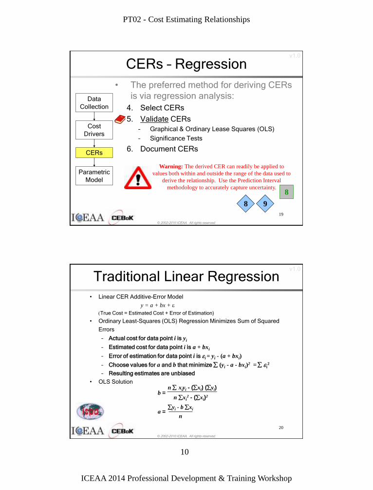
• The preferred method for deriving CERs
is via regression analysis:
4. Select CERs
5. Validate CERs
– Graphical & Ordinary Lease Squares (OLS)
– Significance Tests
6. Document CERs
Cost
Drivers
CERs
Parametric
Model
Data
Collection
Warning: The derived CER can readily be applied to
values both within and outside the range of the data used to
derive the relationship. Use the Prediction Interval
methodology to accurately capture uncertainty.
8 9
8
© 2002-2010 ICEAA. All rights reserved.
v1.0
Traditional Linear Regression
• Linear CER Additive-Error Model
y = a + bx +
(True Cost = Estimated Cost + Error of Estimation)
• Ordinary Least-Squares (OLS) Regression Minimizes Sum of Squared
Errors
– Actual cost for data point i is yi
– Estimated cost for data point i is a + bxi
– Error of estimation for data point i is i = yi - (a + bxi)
– Choose values for a and b that minimize (yi - a - bxi)2 = i
2
– Resulting estimates are unbiased
• OLS Solution
20
b = n xiyi - (xi) (yi)
n xi2 - (xi)
2
yi - b xi
n a =
PT02 - Cost Estimating Relationships
ICEAA 2014 Professional Development & Training Workshop
11
© 2002-2010 ICEAA. All rights reserved.
v1.0 Curve Fitting –
Least-Squares Bet Fit (LSBF)
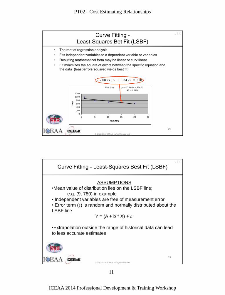
• The root of regression analysis
• Fits independent variables to a dependent variable or variables
• Resulting mathematical form may be linear or curvilinear
• Fit minimizes the square of errors between the specific equation and
the data (least errors squared yields best fit)
21
Unit Cost
0
200
400
600
800
1000
1200
0 5 10 15 20 25
Quantity
Co
st
-17.083 x 15 + 934.22 = 678
Unit Cost y = -17.083x + 934.22
R2 = 0.7826
0
200
400
600
800
1000
1200
0 5 10 15 20 25
Quantity
Co
st
XXX
© 2002-2010 ICEAA. All rights reserved.
v1.0
Curve Fitting - Least-Squares Best Fit (LSBF)
22
ASSUMPTIONS
•Mean value of distribution lies on the LSBF line;
e.g. (9, 780) in example
• Independent variables are free of measurement error
• Error term () is random and normally distributed about the
LSBF line
Y = (A + b * X) +
•Extrapolation outside the range of historical data can lead
to less accurate estimates
PT02 - Cost Estimating Relationships
ICEAA 2014 Professional Development & Training Workshop
12
© 2002-2010 ICEAA. All rights reserved.
v1.0 Curve Fitting –
Least-Squares Bet Fit (LSBF)
23
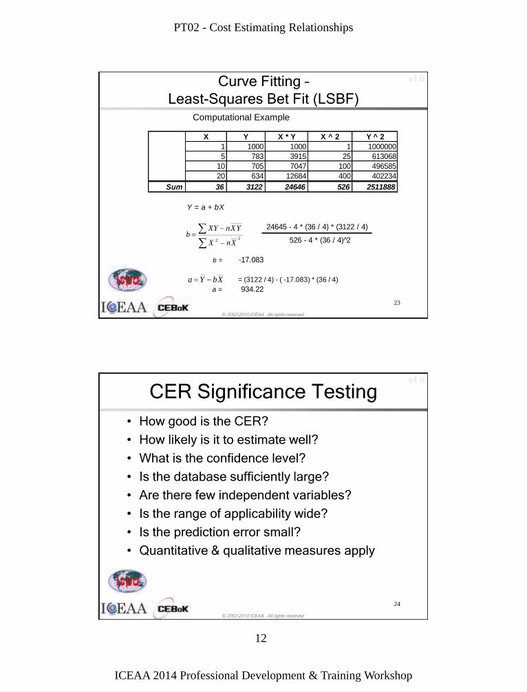
Computational Example
X Y X * Y X ^ 2 Y ^ 2
1 1000 1000 1 1000000
5 783 3915 25 613068
10 705 7047 100 496585
20 634 12684 400 402234
Sum 36 3122 24646 526 2511888
Y = a + bX
24645 - 4 * (36 / 4) * (3122 / 4)
526 - 4 * (36 / 4) 2̂
b = -17.083
= (3122 / 4) - ( -17.083) * (36 / 4)
a = 934.22
XbYa
22 XnX
YXnXYb
© 2002-2010 ICEAA. All rights reserved.
v1.0
CER Significance Testing
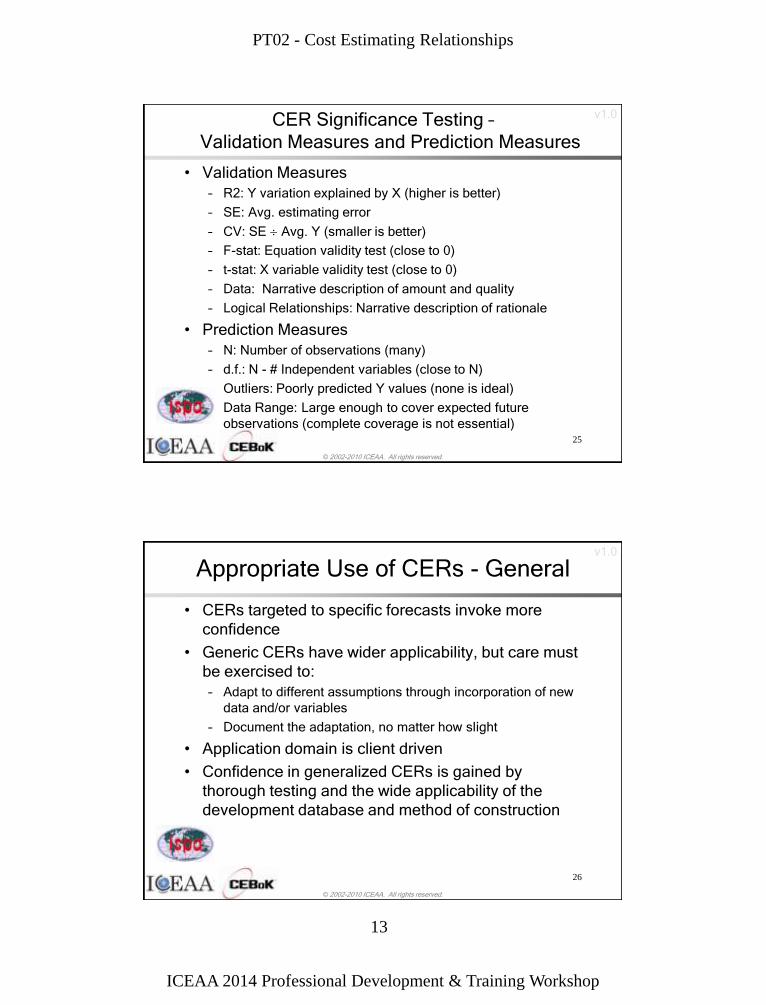
• How good is the CER?
• How likely is it to estimate well?
• What is the confidence level?
• Is the database sufficiently large?
• Are there few independent variables?
• Is the range of applicability wide?
• Is the prediction error small?
• Quantitative & qualitative measures apply
24
PT02 - Cost Estimating Relationships
ICEAA 2014 Professional Development & Training Workshop
13
© 2002-2010 ICEAA. All rights reserved.
v1.0 CER Significance Testing –
Validation Measures and Prediction Measures
• Validation Measures
– R2: Y variation explained by X (higher is better)
– SE: Avg. estimating error
– CV: SE Avg. Y (smaller is better)
– F-stat: Equation validity test (close to 0)
– t-stat: X variable validity test (close to 0)
– Data: Narrative description of amount and quality
– Logical Relationships: Narrative description of rationale
• Prediction Measures
– N: Number of observations (many)
– d.f.: N - # Independent variables (close to N)
– Outliers: Poorly predicted Y values (none is ideal)
– Data Range: Large enough to cover expected future
observations (complete coverage is not essential)
25
© 2002-2010 ICEAA. All rights reserved.
v1.0
Appropriate Use of CERs - General
• CERs targeted to specific forecasts invoke more
confidence
• Generic CERs have wider applicability, but care must
be exercised to:
– Adapt to different assumptions through incorporation of new
data and/or variables
– Document the adaptation, no matter how slight
• Application domain is client driven
• Confidence in generalized CERs is gained by
thorough testing and the wide applicability of the
development database and method of construction
26
PT02 - Cost Estimating Relationships
ICEAA 2014 Professional Development & Training Workshop
14
© 2002-2010 ICEAA. All rights reserved.
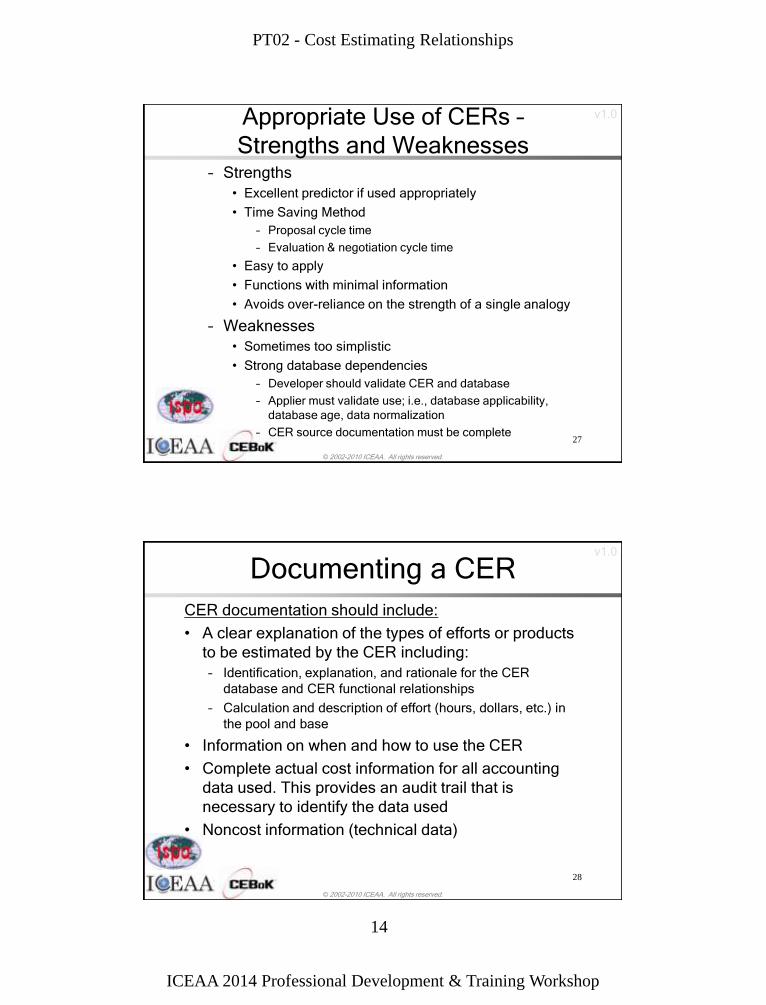
v1.0 Appropriate Use of CERs –
Strengths and Weaknesses – Strengths
• Excellent predictor if used appropriately
• Time Saving Method
– Proposal cycle time
– Evaluation & negotiation cycle time
• Easy to apply
• Functions with minimal information
• Avoids over-reliance on the strength of a single analogy
– Weaknesses
• Sometimes too simplistic
• Strong database dependencies
– Developer should validate CER and database
– Applier must validate use; i.e., database applicability,
database age, data normalization
– CER source documentation must be complete 27
© 2002-2010 ICEAA. All rights reserved.
v1.0
Documenting a CER
CER documentation should include:
• A clear explanation of the types of efforts or products
to be estimated by the CER including:
– Identification, explanation, and rationale for the CER
database and CER functional relationships
– Calculation and description of effort (hours, dollars, etc.) in
the pool and base
• Information on when and how to use the CER
• Complete actual cost information for all accounting
data used. This provides an audit trail that is
necessary to identify the data used
• Noncost information (technical data)
28
PT02 - Cost Estimating Relationships
ICEAA 2014 Professional Development & Training Workshop
15
© 2002-2010 ICEAA. All rights reserved.
v1.0
29
Warning: If you don’t properly account for correlation
between cost elements, your uncertainty will be understated!
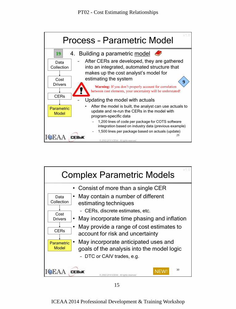
Process – Parametric Model
4. Building a parametric model
– After CERs are developed, they are gathered
into an integrated, automated structure that
makes up the cost analyst’s model for
estimating the system
– Updating the model with actuals
• After the model is built, the analyst can use actuals to
update and re-run the CERs in the model with
program-specific data
– 1,200 lines of code per package for COTS software
integration based on industry data (previous example)
– 1,500 lines per package based on actuals (update)
Cost
Drivers
CERs
Parametric
Model
Data
Collection
9
19
© 2002-2010 ICEAA. All rights reserved.
v1.0
30
Complex Parametric Models
• Consist of more than a single CER
• May contain a number of different
estimating techniques
– CERs, discrete estimates, etc.
• May incorporate time phasing and inflation
• May provide a range of cost estimates to
account for risk and uncertainty
• May incorporate anticipated uses and
goals of the analysis into the model logic
– DTC or CAIV trades, e.g.
Cost
Drivers
CERs
Parametric
Model
Data
Collection
NEW!
PT02 - Cost Estimating Relationships
ICEAA 2014 Professional Development & Training Workshop
16
© 2002-2010 ICEAA. All rights reserved.
v1.0
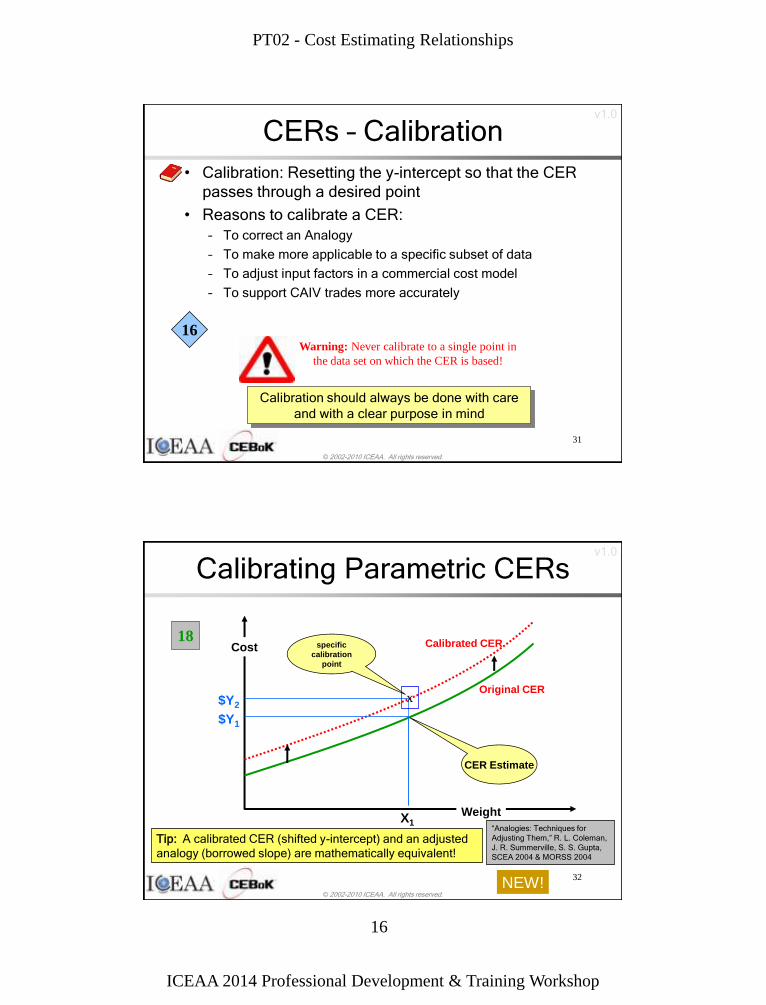
CERs – Calibration
• Calibration: Resetting the y-intercept so that the CER
passes through a desired point
• Reasons to calibrate a CER:
– To correct an Analogy
– To make more applicable to a specific subset of data
– To adjust input factors in a commercial cost model
– To support CAIV trades more accurately
31
Warning: Never calibrate to a single point in
the data set on which the CER is based!
Calibration should always be done with care
and with a clear purpose in mind
16
© 2002-2010 ICEAA. All rights reserved.
v1.0
Calibrating Parametric CERs
32
X1
Original CER
Calibrated CER specific
calibration
point
Weight
Cost
CER Estimate
$Y1
$Y2 x
Tip: A calibrated CER (shifted y-intercept) and an adjusted
analogy (borrowed slope) are mathematically equivalent!
“Analogies: Techniques for
Adjusting Them,” R. L. Coleman,
J. R. Summerville, S. S. Gupta,
SCEA 2004 & MORSS 2004
NEW!
18
PT02 - Cost Estimating Relationships
ICEAA 2014 Professional Development & Training Workshop
17
© 2002-2010 ICEAA. All rights reserved.
v1.0
33
Parametric Process Examples
© 2002-2010 ICEAA. All rights reserved.
v1.0
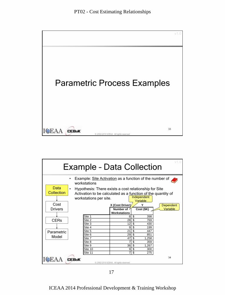
34
X (Cost Driver) Y
Number of
Workstations
Cost ($K)
Site 1 8 398$
Site 2 28 769$
Site 3 12 430$
Site 4 9 199$
Site 5 21 447$
Site 6 29 851$
Site 7 47 1,258$
Site 8 7 359$
Site 9 36 1,267$
Site 10 9 300$
Site 11 7 275$
Example – Data Collection • Example: Site Activation as a function of the number of
workstations
• Hypothesis: There exists a cost relationship for Site
Activation to be calculated as a function of the quantity of
workstations per site. Independent
Variable
Dependent
Variable
Cost
Drivers
CERs
Parametric
Model
Data
Collection
PT02 - Cost Estimating Relationships
ICEAA 2014 Professional Development & Training Workshop
18
© 2002-2010 ICEAA. All rights reserved.
v1.0
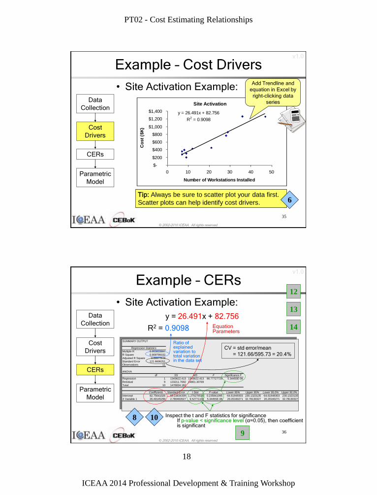
35
Example – Cost Drivers
• Site Activation Example:
Site Activation
y = 26.491x + 82.756
R2 = 0.9098
$-
$200
$400
$600
$800
$1,000
$1,200
$1,400
0 10 20 30 40 50
Number of Workstations Installed
Co
st
($K
)
Tip: Always be sure to scatter plot your data first.
Scatter plots can help identify cost drivers.
Cost
Drivers
CERs
Parametric
Model
Data
Collection
6
Add Trendline and
equation in Excel by
right-clicking data
series
© 2002-2010 ICEAA. All rights reserved.
v1.0
36
Example – CERs
• Site Activation Example:
y = 26.491x + 82.756
SUMMARY OUTPUT
Regression Statistics
Multiple R 0.953833897
R Square 0.909799102
Adjusted R Square 0.89977678
Standard Error 121.6606251
Observations 11
ANOVA
df SS MS F Significance F
Regression 1 1343622.413 1343622.413 90.77727729 5.34455E-06
Residual 9 133211.7692 14801.30769
Total 10 1476834.182
Coefficients Standard Error t Stat P-value Lower 95% Upper 95% Lower 95.0% Upper 95.0%
Intercept 82.75641026 65.14834309 1.270276516 0.235841095 -64.61949303 230.1323135 -64.61949303 230.1323135
X Variable 1 26.49145299 2.780463527 9.52771102 5.34455E-06 20.20160271 32.78130327 20.20160271 32.78130327
Equation Parameters
Inspect the t and F statistics for significance If p-value < significance level (α=0.05), then coefficient
is significant
Ratio of explained variation to total variation in the data set
8
CV = std error/mean
= 121.66/595.73 = 20.4%
Cost
Drivers
CERs
Parametric
Model
Data
Collection R2 = 0.9098
10
9
13
12
14
PT02 - Cost Estimating Relationships
ICEAA 2014 Professional Development & Training Workshop
19
© 2002-2010 ICEAA. All rights reserved.
v1.0
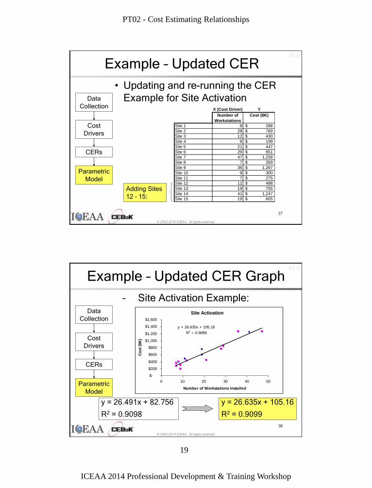
37
Example – Updated CER
• Updating and re-running the CER
Example for Site Activation
Adding Sites
12 – 15:
X (Cost Driver) Y
Number of
Workstations
Cost ($K)
Site 1 8 398$
Site 2 28 769$
Site 3 12 430$
Site 4 9 199$
Site 5 21 447$
Site 6 29 851$
Site 7 47 1,258$
Site 8 7 359$
Site 9 36 1,267$
Site 10 9 300$
Site 11 7 275$
Site 12 11 488$
Site 13 19 755$
Site 14 41 1,247$
Site 15 19 605$
Cost
Drivers
CERs
Parametric
Model
Data
Collection
© 2002-2010 ICEAA. All rights reserved.
v1.0
38
Example – Updated CER Graph
– Site Activation Example:
Site Activation
y = 26.635x + 105.16
R2 = 0.9099
$-
$200
$400
$600
$800
$1,000
$1,200
$1,400
$1,600
0 10 20 30 40 50
Number of Workstations Installed
Co
st
($K
)
y = 26.635x + 105.16
R2 = 0.9099
y = 26.491x + 82.756
R2 = 0.9098
Cost
Drivers
CERs
Parametric
Model
Data
Collection
PT02 - Cost Estimating Relationships
ICEAA 2014 Professional Development & Training Workshop
20
© 2002-2010 ICEAA. All rights reserved.
v1.0
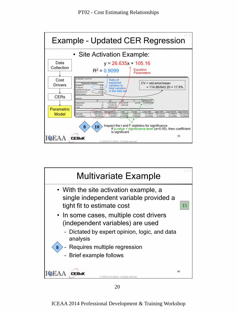
39
8 10
Example – Updated CER Regression
• Site Activation Example:
SUMMARY OUTPUT
Regression Statistics
Multiple R 0.95
R Square 0.91
Adjusted R Square 0.90
Standard Error 114.86
Observations 15
ANOVA
df SS MS F Significance F
Regression 1 1732752.60 1732752.60 131.35 0.000000036
Residual 13 171491.80 13191.68
Total 14 1904244.40
Coefficients Standard Error t Stat P-value Lower 95% Upper 95% Lower 95.0% Upper 95.0%
Intercept 105.164101 55.527605 1.893907 0.080704 -14.795974 225.124176 -14.795974 225.124176
X Variable 1 26.635441 2.324029 11.460888 0.000000 21.614681 31.656200 21.614681 31.656200
Cost
Drivers
CERs
Parametric
Model
Data
Collection y = 26.635x + 105.16
Equation Parameters
Inspect the t and F statistics for significance If p-value < significance level (α=0.05), then coefficient
is significant
Ratio of explained variation to total variation in the data set
CV = std error/mean
= 114.86/643.20 = 17.9%
R2 = 0.9099
© 2002-2010 ICEAA. All rights reserved.
v1.0
40
Multivariate Example
• With the site activation example, a
single independent variable provided a
tight fit to estimate cost
• In some cases, multiple cost drivers
(independent variables) are used
– Dictated by expert opinion, logic, and data
analysis
– Requires multiple regression
– Brief example follows
8
15
PT02 - Cost Estimating Relationships
ICEAA 2014 Professional Development & Training Workshop
21
© 2002-2010 ICEAA. All rights reserved.
v1.0
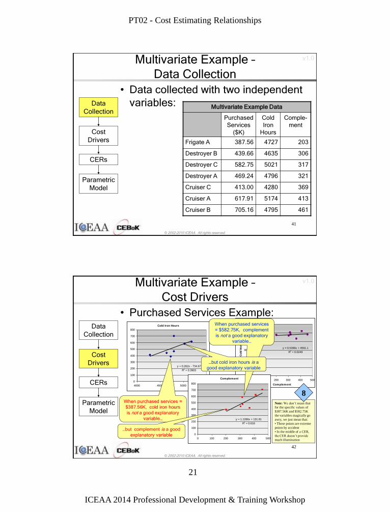
41
Multivariate Example –
Data Collection
• Data collected with two independent
variables:
Multivariate Example Data
Purchased
Services
($K)
Cold
Iron
Hours
Comple-
ment
Frigate A 387.56 4727 203
Destroyer B 439.66 4635 306
Destroyer C 582.75 5021 317
Destroyer A 469.24 4796 321
Cruiser C 413.00 4280 369
Cruiser A 617.91 5174 413
Cruiser B 705.16 4795 461
Cost
Drivers
CERs
Parametric
Model
Data
Collection
© 2002-2010 ICEAA. All rights reserved.
v1.0
42
Note: We don’t mean that
for the specific values of
$387.56K and $582.75K
the variables magically go
awry, we just mean that:
• Those points are extreme
points by accident
• In the middle of a CER,
the CER doesn’t provide
much illumination
Cold Iron Hours
y = 0.262x - 734.67
R2 = 0.3903
0
100
200
300
400
500
600
700
800
4000 4500 5000 5500
y = 0.5399x + 4591.1
R2 = 0.0249
0
1000
2000
3000
4000
5000
6000
0 100 200 300 400 500
Complement
Co
ld Ir
on
Complement
y = 1.1266x + 131.81
R2 = 0.616
0
100
200
300
400
500
600
700
800
0 100 200 300 400 500
When purchased services
= $582.75K, complement
is not a good explanatory
variable…
Multivariate Example –
Cost Drivers
• Purchased Services Example:
Cost
Drivers
CERs
Parametric
Model
Data
Collection
…but cold iron hours is a
good explanatory variable
When purchased services =
$387.56K, cold iron hours
is not a good explanatory
variable…
…but complement is a good
explanatory variable
8
PT02 - Cost Estimating Relationships
ICEAA 2014 Professional Development & Training Workshop
22
© 2002-2010 ICEAA. All rights reserved.
v1.0
43
SUMMARY OUTPUT
Regression Statistics
Multiple R 0.934462283
R Square 0.873219758
Adjusted R Square 0.809829638
Standard Error 52.13001587
Observations 7
ANOVA
df SS MS F Significance F
Regression 2 74869.97435 37434.98717 13.77532882 0.01607323
Residual 4 10870.15422 2717.538555
Total 6 85740.12857
Coefficients Standard Error t Stat P-value Lower 95% Upper 95% Lower 95.0% Upper 95.0%
Intercept -854.2676929 358.213134 -2.384802822 0.075593456 -1848.828855 140.2934695 -1848.828855 140.2934695
Cold Iron Hours 0.214824888 0.075578629 2.842402553 0.046753766 0.004984539 0.424665237 0.004984539 0.424665237
Complement 1.009958432 0.258711303 3.903804826 0.017485119 0.291659214 1.728257649 0.291659214 1.728257649
8 10
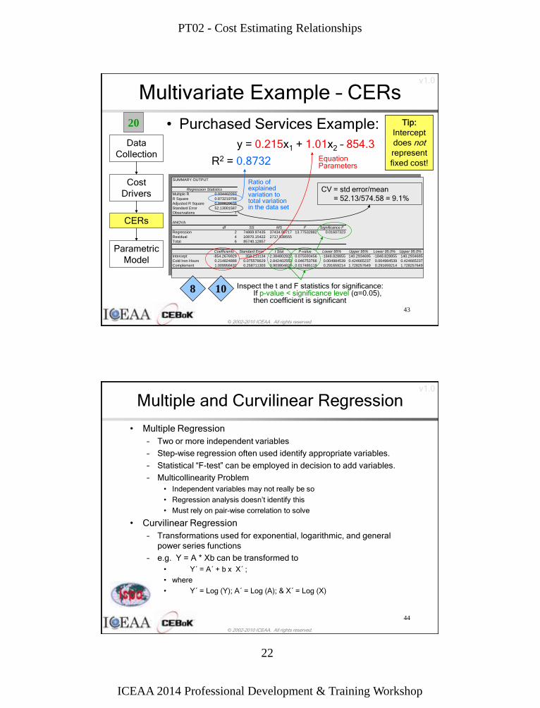
Multivariate Example – CERs
• Purchased Services Example:
y = 0.215x1 + 1.01x2 – 854.3 Equation Parameters
Inspect the t and F statistics for significance: If p-value < significance level (α=0.05),
then coefficient is significant
Ratio of explained variation to total variation in the data set
CV = std error/mean
= 52.13/574.58 = 9.1%
Cost
Drivers
CERs
Parametric
Model
Data
Collection R2 = 0.8732
Tip:
Intercept
does not represent
fixed cost!
20
© 2002-2010 ICEAA. All rights reserved.
v1.0
Multiple and Curvilinear Regression
• Multiple Regression
– Two or more independent variables
– Step-wise regression often used identify appropriate variables.
– Statistical “F-test” can be employed in decision to add variables.
– Multicollinearity Problem
• Independent variables may not really be so
• Regression analysis doesn’t identify this
• Must rely on pair-wise correlation to solve
• Curvilinear Regression
– Transformations used for exponential, logarithmic, and general
power series functions
– e.g. Y = A * Xb can be transformed to
• Y´ = A´ + b x X´ ;
• where
• Y´ = Log (Y); A´ = Log (A); & X´ = Log (X)
44
PT02 - Cost Estimating Relationships
ICEAA 2014 Professional Development & Training Workshop
23
© 2002-2010 ICEAA. All rights reserved.
v1.0
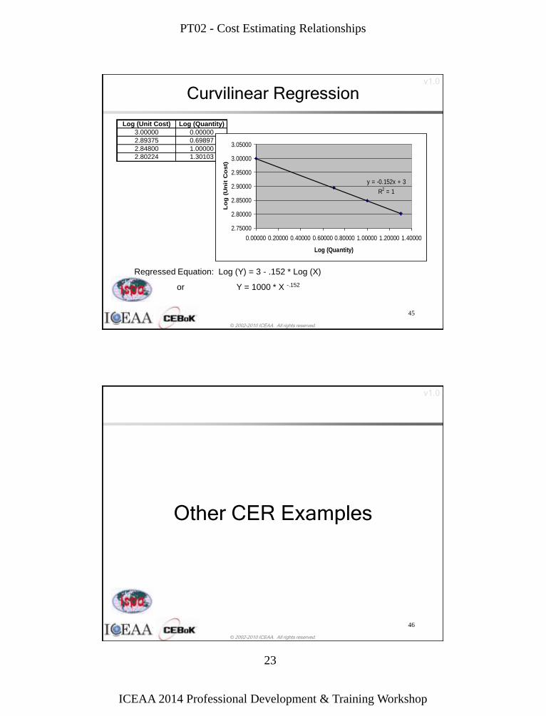
Curvilinear Regression
45
Log (Unit Cost) Log (Quantity)
3.00000 0.00000
2.89375 0.69897
2.84800 1.00000
2.80224 1.30103
y = -0.152x + 3
R2 = 1
2.75000
2.80000
2.85000
2.90000
2.95000
3.00000
3.05000
0.00000 0.20000 0.40000 0.60000 0.80000 1.00000 1.20000 1.40000
Log (Quantity)
Lo
g (
Un
it C
ost)
Regressed Equation: Log (Y) = 3 - .152 * Log (X)
or Y = 1000 * X -.152
© 2002-2010 ICEAA. All rights reserved.
v1.0
46
Other CER Examples
PT02 - Cost Estimating Relationships
ICEAA 2014 Professional Development & Training Workshop
24
© 2002-2010 ICEAA. All rights reserved.
v1.0
Cost Improvement Curve
• Also known as the Learning Curve
• Mathematical form: Y = A * X b
– Y is either unit cost or average unit cost
– A is first unit cost (T1)
– X is unit number
– b is improvement or learning factor
• Learning Curve Interpretation
– Constant cost improvement with each doubling of
quantity (e.g. 90% LC = 10% improvement with
every doubling of quantity)
– b = ln(LC) ln(2)
47
© 2002-2010 ICEAA. All rights reserved.
v1.0
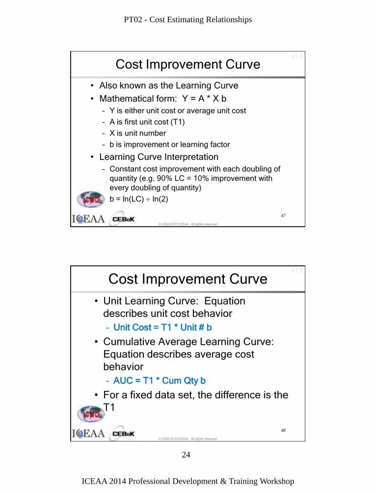
Cost Improvement Curve
• Unit Learning Curve: Equation
describes unit cost behavior
– Unit Cost = T1 * Unit # b
• Cumulative Average Learning Curve:
Equation describes average cost
behavior
– AUC = T1 * Cum Qty b
• For a fixed data set, the difference is the
T1
48
PT02 - Cost Estimating Relationships
ICEAA 2014 Professional Development & Training Workshop
25
© 2002-2010 ICEAA. All rights reserved.
v1.0
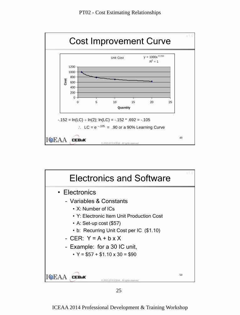
Cost Improvement Curve
49
Unit Cost y = 1000x-0.152
R2 = 1
0
200
400
600
800
1000
1200
0 5 10 15 20 25
Quantity
Co
st
-.152 = ln(LC) ln(2); ln(LC) = -.152 * .692 = -.105
LC = e –.105 = .90 or a 90% Learning Curve
© 2002-2010 ICEAA. All rights reserved.
v1.0
Electronics and Software
• Electronics
– Variables & Constants
• X: Number of ICs
• Y: Electronic Item Unit Production Cost
• A: Set-up cost ($57)
• b: Recurring Unit Cost per IC ($1.10)
– CER: Y = A + b x X
– Example: for a 30 IC unit,
• Y = $57 + $1.10 x 30 = $90
50
PT02 - Cost Estimating Relationships
ICEAA 2014 Professional Development & Training Workshop
26
© 2002-2010 ICEAA. All rights reserved.
v1.0
Construction/Reconstruction
• Variables & Constants
– X1: Area (square feet)
– a: area coefficient ($75 per square foot)
– X2: # Rooms
– b: rooms coefficient ($5,000 per room)
– C: Home type (1 for tract, 1.33 for semi-custom, 1.5 for
custom)
– Y: Construction Cost
• CER: Y = C x (a x X1 + b x X2)
• Example: A 12 room, 2500 square foot, semi-custom
built home,
• 1.5 x ($75 x 2500 + $5000 x 12) = $371,250
51
© 2002-2010 ICEAA. All rights reserved.
v1.0
Software
• Variables & Constants
– X: Thousands of Delivered Source Instructions
– A: Type coefficient; 3.2, 3.0, or 2.8
– b: Type Exponent; 1.05, 1.12, or 1.2
– Y: Labor months of development effort
• CER: Y = A x Xb
• Example: For a 40,000 DSI, Type 3 program
• 2.8 x 401.2 = 234.2 labor months
52
PT02 - Cost Estimating Relationships
ICEAA 2014 Professional Development & Training Workshop
27
© 2002-2010 ICEAA. All rights reserved.
v1.0
53
CER Validation
© 2002-2010 ICEAA. All rights reserved.
v1.0
Evaluating CERs - Criteria
– Logical data relationships
– Uses adequate data
– Evidence of strong relationships
– Consistent and valid application
– Cost drivers (variables) make logical sense
– Driving data should be accessible for both CER
development and implementation
– Driver list should be comprehensive
– Excluded outliers and rationale for exclusion
should be identified
– Meets customer needs
54

PT02 - Cost Estimating Relationships
ICEAA 2014 Professional Development & Training Workshop
28
© 2002-2010 ICEAA. All rights reserved.
v1.0
Evaluating CERs – Criteria
– Validation
• Establishes the CER as a credible estimating
method
• Validation = Documented Consistent Accuracy
– Requires periodic testing
– CER updated when testing indicates need
• Validation falls to CER developer
• Certification falls to CER applier
55
© 2002-2010 ICEAA. All rights reserved.
v1.0
Evaluating CERs – Credible Data
• Credible Data
– Assembling a quality database is the single most important and
time consuming step
– Database must be encompassing but not overwhelming
– Historical data is preferred
– Data normalization must be consistent
– Formats for data types should be consistent (Cost, Technical,
Programmatic)
– Database must be fed and cared for
• Strength of Data Relationships
– Can be judged with Statistical tests
– R2 and Standard Error are most popular strength tests
• Complementary
• R2 measures the degree to which the independent variables describe
variation in the historical data
• Standard error measures average error |predicted - actual| in the
historical data
56

PT02 - Cost Estimating Relationships
ICEAA 2014 Professional Development & Training Workshop
29
© 2002-2010 ICEAA. All rights reserved.
v1.0
57
Parametric Estimating Summary
• Parametric Estimating uses cost estimating relationships (CERs) based on historical data to predict cost
• Until actual cost data are available, the use of parametric costing techniques is the preferred approach
• Parametric estimating process – Collecting Data
– Identifying Cost Drivers
– Developing CERs
– Building a parametric model
• OTS Cost Models are convenient to use but must be applied with caution
4
6
8
© 2002-2010 ICEAA. All rights reserved.
v1.0
58
Resources
• DoD 5000.4-M, Department of Defense Manual Cost Analysis Guidance and Procedures, December 1992 – http://west.dtic.mil/whs/directives/corres/pdf/500004m.pdf
• International Society of Parametric Analysts (ISPA), Parametric Estimating Handbook, 4th Edition, April 2008 – http://www.ispa-cost.org/ISPA_PEH_4th_ed_Final.pdf
• “Cost Response Curves - Their generation, their use in IPTs, Analyses of Alternatives, and Budgets,” K.J. Allison, K.E. Crum, R.L. Coleman, R.G. Klion, DoDCAS, 1996
• “Analogies: Techniques for Adjusting Them,” R. L. Coleman, J. R. Summerville, S. S. Gupta, SCEA 2004 & MORSS 2004