ceae.colorado.educeae.colorado.edu/~sture/plaxis/slides/course notes on... · web viewusage of the...

Non-Linear Hyperbolic Model & Parameter Selection

NON-LINEAR HYPERBOLIC MODEL & PARAMETER SELECTION

(Introduction to the Hardening Soil Model)

(following initial development by Tom Schanz at Bauhaus-Universität Weimar, Germany)

Computational Geotechnics

Course ‘Computational Geotechnics’ 1


Contents

IntroductionStiffness ModulusTriaxial DataPlasticityHS-Cap-ModelSimulation of Oedometer and Triaxial Tests on Loose and Dense SandsSummary



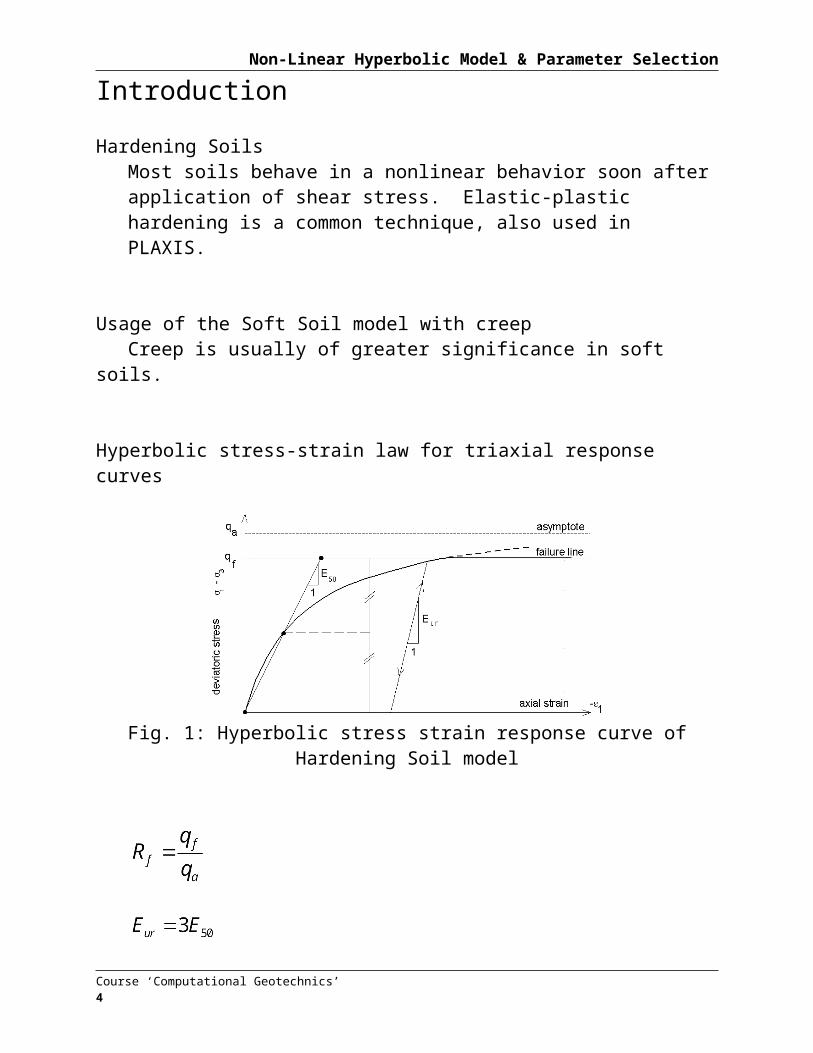
Introduction

Hardening SoilsMost soils behave in a nonlinear behavior soon after application of shear stress. Elastic-plastic hardening is a common technique, also used in PLAXIS.

Usage of the Soft Soil model with creepCreep is usually of greater significance in soft soils.

Hyperbolic stress-strain law for triaxial response curves

Fig. 1: Hyperbolic stress strain response curve of Hardening Soil model

(standard PLAXIS setting Version 7)



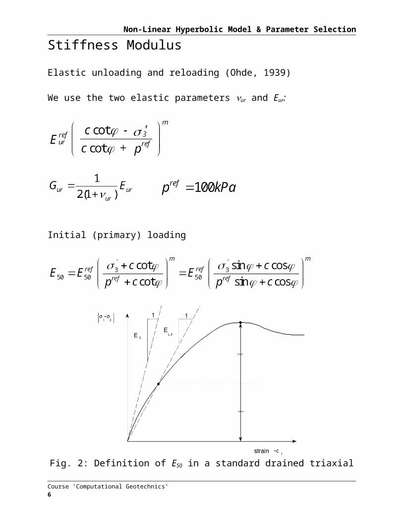
Stiffness Modulus

Elastic unloading and reloading (Ohde, 1939)

We use the two elastic parameters ur and Eur:

Initial (primary) loading

Fig. 2: Definition of E50 in a standard drained triaxial experiment



Stiffness Modulus

Oedometer tests

Fig. 3: Definition of the normalized oedometric stiffness

Fig. 4: Values for m from oedometer test versus initial porosity n0

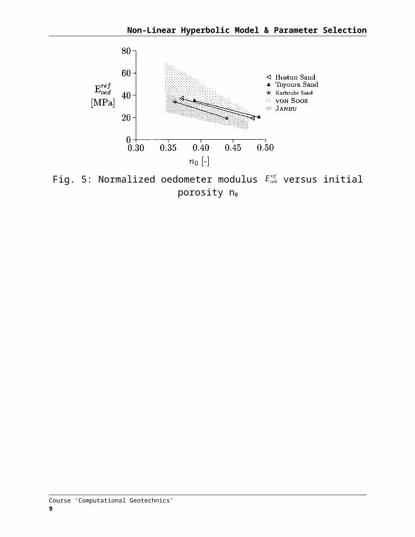
Fig. 5: Normalized oedometer modulus versus initial porosity n0



Stiffness Modulus

Triaxial tests

Fig. 6: Normalized oedometric stiffness for various soil classes (von Soos, 1991)



Stiffness Modulus

Fig. 7: Values for m obtained from triaxial test versus initial porosity n0

Fig. 8: Normalized triaxial modulus versus initial porosity n0



Stiffness Modulus

Summary of data for sand: Vermeer & Schanz (1997)

Fig. 9: Comparison of normalized stiffness moduli from oedometer and triaxial tests

Engineering practice: mostly data on Eoed

Test data:

(standard setting PLAXIS version 7)



Triaxial Data on p 21p

Fig. 10: Equi-g lines (Tatsuoka, 1972) for dense Toyoura Sand

Fig. 11: Yield and failure surfaces for the Hardening Soil model



Plasticity

Yield and hardening functions

3D extension

In order to extent the model to general 3D states in terms of stress, we use a modified expression for in terms of and the mobilized angle of internal

friction

with

where



Plasticity

Plastic potential and flow rule

with

where

m

mM

sin3

sin6*

Flow rule

with

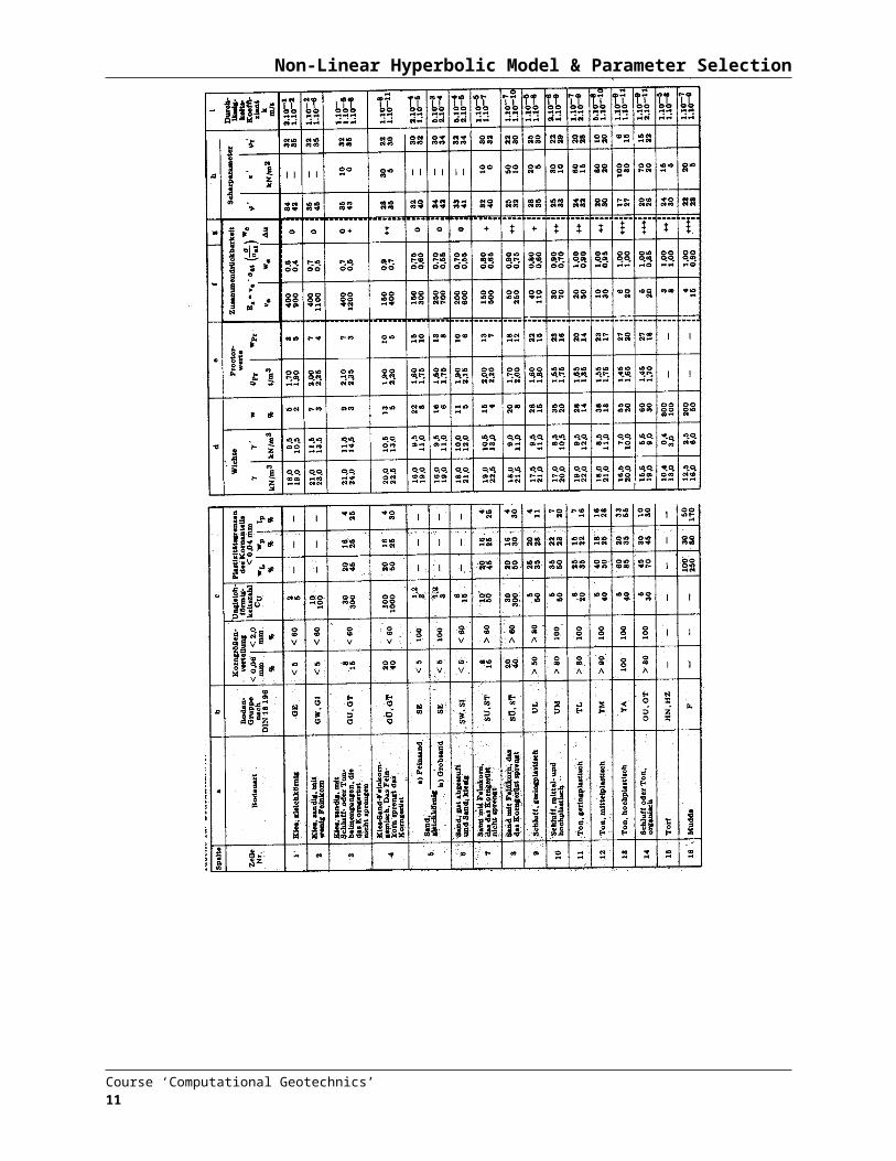
Table 1: Primary soil parameters and standard PLAXIS settingsC [kPa] j’ [o] [o] E50 [Mpa] 0 30-40 0-10 40 Eur = 3 E50 Vur = 0.2 Rf = 0.9 m = 0.5 Pref = 100 kPa



Plasticity

Hardening soil response in drained triaxial experiments

Fig. 12: Results of drained triaxial loading: stress-strain relations (s3 = 100 kPa)

Fig. 13: Results of drained triaxial loading: axial-volumetric strain relations (s3 = 100 kPa)



Plasticity

Undrained hardening soil analysis

Method A: switch to drainedInput:

Method B: switch to undrainedInput:

Interesting in case you have data on Cu and not no C’ and ’

Assume and use graph by Duncan & Buchignani (1976) to estimate Eu

Fig. 14: Undrained Hardening Soil analysis


2cu

Eu 1.4 E50


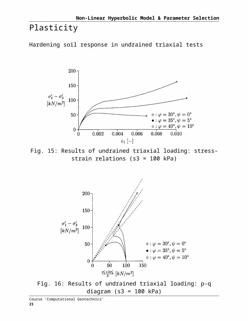
Plasticity

Hardening soil response in undrained triaxial tests

Fig. 15: Results of undrained triaxial loading: stress-strain relations (s3 = 100 kPa)

Fig. 16: Results of undrained triaxial loading: p-q diagram (s3 = 100 kPa)



HS-Cap-Model

Cap yield surface

Flow rule(Associated flow)

Hardening law

For isotropic compression we assume

With

For isotropic compression we have q = 0 and it follows from

For the determination of, we use another consistency condition:



HS-Cap-Model

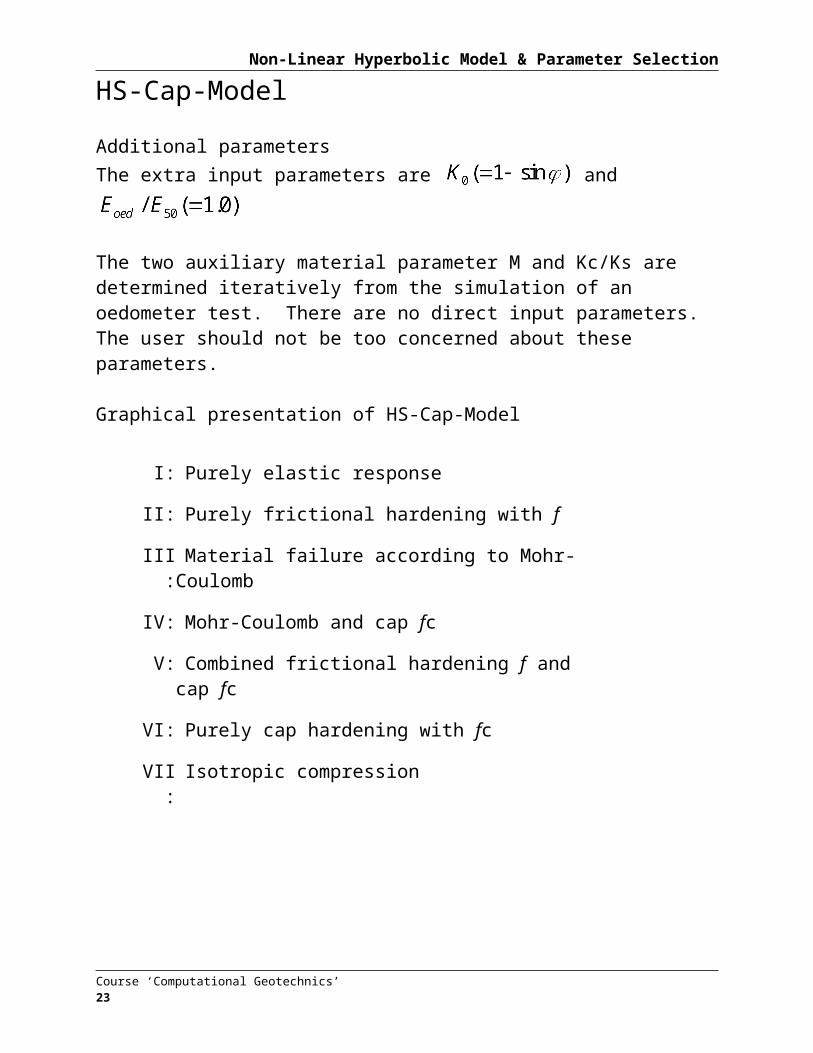
Additional parametersThe extra input parameters are and

The two auxiliary material parameter M and Kc/Ks are determined iteratively from the simulation of an oedometer test. There are no direct input parameters. The user should not be too concerned about these parameters.

Graphical presentation of HS-Cap-Model

I: Purely elastic response

II: Purely frictional hardening with f

III: Material failure according to Mohr-Coulomb

IV: Mohr-Coulomb and cap fc

V: Combined frictional hardening f and cap fc

VI: Purely cap hardening with fc

VII: Isotropic compression

Fig. 17: Yield surfaces of the extended HS model in p-q-space (left) and in the deviatoric plane (right)


1

2 3


HS-Cap-Model

Fig. 18: Yield surfaces of the extended HS model in principal stress space


1 = 2 = 3


Simulation of Oedometer and Triaxial Tests on Loose and Dense Sands

Fig. 19: Comparison of calculated (•) and measured triaxial tests on loose Hostun Sand

Fig. 20: Comparison of calculated (•) and measured oedometer tests on loose Hostun Sand



Simulation of Oedometer and Triaxial Tests on Loose and Dense Sands

Fig. 21: Comparison of calculated (•) and measured triaxial tests on dense Hostun Sand

Fig. 22: Comparison of calculated (•) and measured oedometer tests on dense Hostun Sand



Summary

Main characteristicsPressure dependent stiffnessIsotropic shear hardeningUltimate Mohr-Coulomb failure conditionNon-associated plastic flowAdditional cap hardening

HS-model versus MC-model

As in Mohr-Coulomb model

Normalized primary loading stiffness

Unloading / reloading Poisson’s ratio

Normalized unloading / reloading stiffness

Power in stiffness laws

Failure ratio



Exercise 1: Calibration of the HS-Cap-Model for Loose and Dense Sand

Oedometer and triaxial shear experimental data for both loose and dense sands are given in Figs. 23 – 26.

Table 2: Parameters for loose and dense sand vur m j

loose 0.25 0.65 34o 0o 1.0 3.0 16dense 0.25 0.65 41o 14o 0.9 3.0 35 MPa

Proceed according to the following steps:

Use Ko = 1 – sin and Eoed/E50 according to Table 2 in the advanced material parameter input in PLAXIS.

For both simulations use an axis-symmetric mesh (1x 1 [m]) with a coarse element density. Change loading and boundary conditions according to the test conditions.

Simulation of oedmoter tests with unloading for unloading for maximum axial stress.

Loose sand: Dense sand:

If necessary improve given material parameters to obtain a more realistic response.

Check triaxial tests with the parameters obtained from the oedometer simulation.




Results for loose sand

Fig. 23: Triaxial tests on loose Hostun Sand

Fig. 24: Oedometer tests on loose Hostun Sand




Results for dense sand

Fig. 25: Triaxial tests on dense Hostun Sand

Fig. 26: Oedometer tests on dense Hostun Sand


ceae.colorado.educeae.colorado.edu/~sture/plaxis/slides/course notes on... · web viewusage of the...

Documents