ce417: introduction to artificial intelligence sharif...

CE417: Introduction to Artificial IntelligenceSharif University of TechnologySpring 2013

Course material: “Artificial Intelligence: A Modern Approach”, 3rd Edition, Chapter 4

Soleymani

Beyond Classical Search

Outline Local search algorithms Hill-climbing search Simulated annealing search Local beam search Genetic algorithms

Searching in continuous spaces

Searching in more complex environments non-deterministic environments partially observable environments unknown environments

2

Sample problems for local & systematic search Path to goal is important Theorem proving Route finding 8-Puzzle Chess

Goal state itself is important 8 Queens TSP VLSI Layout Job-Shop Scheduling Automatic program generation

3

State-space landscape Local search algorithms explore the landscape Solution:A state with the optimal value of the objective function

2-d state space

4

Example: n-queens Put n queens on an n × n board with no two queens on

the same row, column, or diagonal What is state-space? What is objective function?

5

Local search: 8-queens problem States: 8 queens on the board, one per column (88 ≈ 17 ) Successors(s): all states resulted from by moving a single queen to

another square of the same column (8 × 7 = 56) Cost function ℎ(s): number of queen pairs that are attacking each

other, directly or indirectly Global minimum: ℎ = 0ℎ( ) = 17 successors objective values

Red: best successors6

Hill-climbing search Node only contains the state and the value of objective

function in that state (not path) Search strategy: steepest ascent among immediate

neighbors until reaching a peak

Current node is replaced by the best successor (if it is better than current node)

7

Hill-climbing search is greedy Greedy local search: considering only one step ahead and

select the best successor state (steepest ascent) Rapid progress toward a solution

Usually quite easy to improve a bad solution

Optimal when starting in one of these states

8

Hill-climbing search problems

9

Local maxima: a peak that is not global max Plateau: a flat area (flat local max, shoulder)

Ridges: a sequence of local max that is verydifficult for greedy algorithm to navigate

Hill-climbing search problem: 8-queens From random initial state, 86% of the time getting stuck on average, 4 steps for succeeding and 3 steps for getting stuck

ℎ( ) = 17Five steps

ℎ( ) = 1

10

Hill-climbing search problem: TSP

11

Start with any complete tour, perform pairwise exchanges Variants of this approach get within 1% of optimal very quickly

with thousands of cities

Variants of hill-climbing Trying to solve problem of hill-climbing search Sideways moves Stochastic hill climbing

First-choice hill climbing

Random-restart hill climbing

12

Sideways move Sideways move: plateau may be a shoulder so keep going

sideways moves when there is no uphill move Problem: infinite loop where flat local max

Solution: upper bound on the number of consecutive sideways moves

Result on 8-queens: Limit = 100 for consecutive sideways moves

94% success instead of 14% success on average, 21 steps when succeeding and 64 steps when failing

13

Stochastic hill climbing Randomly chooses among the available uphill moves

according to the steepness of these moves ( ’) is an increasing function of ℎ( ’) − ℎ( )

First-choice hill climbing: generating successors randomlyuntil one better than the current state is found

Good when number of successors is high

14

Random-restart hill climbing All previous versions are incomplete Getting stuck on local max

while state ≠ goal dorun hill-climbing search from a random initial state

: probability of success in each hill-climbing search Expected no of restarts = 1/ Expected no of steps = 1⁄ − 1 × +

: average number of steps in a failure : average number of steps for the success

Result on 8-queens: ≈ 0.14 ⇒ 1/ ≈ 7 iterations

7 − 1 × 3 + 4 ≈ 22 steps For 3 × 10 queens needs less than 1 minute

Using also sideways moves: ≈ 0.94 ⇒ 1/ ≈ 1.06 iterations 1.06 − 1 × 64 + 21 ≈ 26 steps

15

Effect of land-scape shape on hill climbing Shape of state-space land-scape is important: Few local max and platea: random-restart is quick Real problems land-scape is usually unknown a priori NP-Hard problems typically have an exponential number of

local maxima Reasonable solution can be obtained after a small no of restarts

16

Simulated Annealing (SA) Search Hill climbing: move to a better state Efficient, but incomplete (can stuck in local maxima)

Random walk: move to a random successor Asymptotically complete, but extremely inefficient

Idea: Escape local maxima by allowing some "bad"moves but gradually decrease their frequency. More exploration at start and gradually hill-climbing become

more frequently selected strategy

17

SA relation to annealing in metallurgy

18

In SA method, each state s of the search space isanalogous to a state of some physical system

E(s) to be minimized is analogous to the internalenergy of the system

The goal is to bring the system, from an arbitrary initialstate, to an equilibrium state with the minimum possibleenergy.

19

Pick a random successor ofthe current state

If it is better than thecurrent state go to it

Otherwise, accept thetransition with a probability

( ) = ℎ [ ] is a decreasing seriesE(s): objective function

Probability of state transition

( ( ) ( ))/ ( ) Probability of “un-optimizing” ( )

random movements depends on badness of move andtemperature Badness of movement: worse movements get less probability Temperature

High temperature at start: higher probability for bad random moves Gradually reducing temperature: random bad movements become more

unlikely and thus hill-climbing moves increase

20

A successor of

SA as a global optimization method

21

Theoretical guarantee: If decreases slowlyenough, simulated annealing search will converge to aglobal optimum (with probability approaching 1)

Practical? Time required to ensure a significantprobability of success will usually exceed the time ofa complete search

Local beam search Keep track of states Instead of just one in hill-climbing and simulated annealing

22

Start with randomly generated statesLoop:

All the successors of all k states are generatedIf any one is a goal state then stopelse select the k best successors from the complete list of successors and repeat.

Local beam search

23

Is it different from running high-climbing with randomrestarts in parallel instead of in sequence? Passing information among parallel search threads

Problem: Concentration in a small region after someiterations Solution: Stochastic beam search

Choose k successors at random with probability that is an increasingfunction of their objective value

Genetic Algorithms

24

A variant of stochastic beam search Successors can be generated by combining two parent states

rather than modifying a single state

Natural Selection

25

There is competition among living things More are born than survive and reproduce

Reproduction occurs with variation This variation is heritable

Selection determines which individuals enter the adultbreeding population This selection is done by the environment Those which are best suited or fitted reproduce They pass these well suited characteristics on to their young

“Survival of the fittest” means those who have the mostoffspring that reproduce

Natural Selection

26

Natural Selection: “Variations occur in reproduction and willbe preserved in successive generations approximately inproportion to their effect on reproductive fitness”

Genetic Algorithms: inspiration by natural selection State: organism

Objective value: fitness (populate the next generationaccording to its value)

Successors: offspring

27

Genetic Algorithm (GA) A state (solution) is represented as a string over a finite alphabet

Like a chromosome containing genes

Start with k randomly generated states (population)

Evaluation function to evaluate states (fitness function) Higher values for better states

Combining two parent states and getting offsprings (cross-over) Cross-over point can be selected randomly

Reproduced states can be slightly modified (mutation)

The next generation of states is produced by selection (based on fitnessfunction), crossover, and mutation

28

Chromosome & Fitness: 8-queens

29

2 4 7 4 8 5 5 2

Describe the individual (or state) as a string

Fitness function: number of non-attacking pairs of queens 24 for above figure

Genetic operators: 8-queens Cross-over: To select some part of the state from one parent

and the rest from another.

30

6 7 2 4 7 5 8 8 7 5 2 5 1 4 4 7 6 7 2 5 1 4 4 7

Genetic operators: 8-queens Cross-over: To select some part of the state from one parent

and the rest from another.

31

6 7 2 4 7 5 8 8 7 5 2 5 1 4 4 7 6 7 2 5 1 4 4 7

Genetic operators: 8-queens

32

Mutation: To change a small part of one state with a smallprobability.

6 7 2 5 1 4 4 7 6 7 2 5 1 3 4 7

Genetic operators: 8-queens

33

Mutation: To change a small part of one state with a smallprobability.

6 7 2 5 1 4 4 7 6 7 2 5 1 3 4 7

A Genetic algorithm diagram

35

Start

Generate initial population

Individual Evaluation

Crossover

Mutation

StopCriteria?

SolutionYes

Selection

6 7 2 4 7 5 8 8

3 1 2 8 2 5 6 6

8 1 4 2 5 3 7 1…

A variant of genetic algorithm: 8-queens

Fitness function: number of non-attacking pairs of queens min = 0, max = 8 × 7/2 = 28 Reproduction rate(i) = ( )/ ∑ ( )

e.g., 24/(24+23+20+11) = 31%

36

(a)

Initial Population

(b)

Fitness Function

(c)

Selection

(d)

Crossover

(e)

Mutation

24

23

20

11

29%

31%

26%

14%

32752411

24748552

32752411

24415124

32748552

24752411

32752124

24415411

32252124

24752411

32748152

24415417

24748552

32752411

24415124

32543213

A variant of genetic algorithm: 8-queens

Fitness function: number of non-attacking pairs of queens min = 0, max = 8 × 7/2 = 28 Reproduction rate(i) = ( )/ ∑ ( )

e.g., 24/(24+23+20+11) = 31%

37

(a)

Initial Population

(b)

Fitness Function

(c)

Selection

(d)

Crossover

(e)

Mutation

24

23

20

11

29%

31%

26%

14%

32752411

24748552

32752411

24415124

32748552

24752411

32752124

24415411

32252124

24752411

32748152

24415417

24748552

32752411

24415124

32543213

Genetic algorithm properties

38

Why does a genetic algorithm usually take large steps inearlier generations and smaller steps later? Initially, population individuals are diverse

Cross-over operation on different parent states can produce a statelong a way from both parents

More similar individuals gradually appear in the population

Cross-over as a distinction property of GA Ability to combine large blocks of genes evolved independently

Representation has an important role in benefit of incorporatingcrossover operator in GA

Local search in continuous spaces Infinite number of successor states

E.g., select locations for 3 airports such that sum of squared distances from each city to its nearest airport is minimized ( 1, 1) , ( 2, 2) , ( 3, 3) ( 1, 1, 2, 2, 3, 3) = ∑ ∑ ( − ) +( − )∈

Approach 1: Discretization Just change variable by ±

E.g., 6×2 actions for airport example

Approach 2: Continuous optimization = 0 (only for simple cases) Gradient ascent 1 ( )t t tf x x x

1 2

, ,...,d

f f ffx x x

Gradient ascent

40

1 ( )t t tf x x x

Local search problems also in continuous spaces Random restarts and simulated annealing can be useful Higher dimensions raises the rate of getting lost

Gradient ascent (step size)

41

Adjusting in gradient descent Line search Newton-Raphson

1 1( ) ( )t t t tf f x x H x x

2ij i jH f x x

Local search vs. systematic search

Systematic search Local search

Solution Path from initial state to the goal Solution state itself

Method Systematically trying different paths from an initial state

Keeping a single or more "current" states and trying to improve them

State space Usually incremental Complete configuration

Memory Usually very high Usually very little (constant)

Time Finding optimal solutions in small state spaces

Finding reasonable solutions in large or infinite (continuous) state spaces

Scope Search Search & optimization problems

42

Searching in non-deterministic, partiallyobservable and unknown environments

43

Problem types Deterministic and fully observable (single-state problem)

Agent knows exactly its state even after a sequence of actions Solution is a sequence

Non-observable or sensor-less (conformant problem) Agent’s percepts provide no information at all Solution is a sequence

Nondeterministic and/or partially observable (contingencyproblem) Percepts provide new information about current state Solution can be a contingency plan (tree or strategy) and not a sequence Often interleave search and execution

Unknown state space (exploration problem)

44

More complex than single-state problem

45

Searching with nondeterministic actions

Searching with partial observations

Online search & unknown environment

Non-deterministic or partially observable env.

46

Perception become useful Partially observable

To narrow down the set of possible states for the agent

Non-deterministic To show which outcome of the action has occurred

Future percepts can not be determined in advance

Solution is a contingency plan A tree composed of nested if-then-else statements What to do depending on what percepts are received

Now, we focus on an agent design that finds a guaranteed planbefore execution (not online search)

Searching with non-deterministic actions In non-deterministic environments, the result of an action

can vary. Future percepts can specify which outcome has occurred.

Generalizing the transition function : × → 2 instead of : × →

Search tree will be an AND-OR tree. Solution will be a sub-tree containing a contingency plan

(nested if-then-else statements)

47

Erratic vacuum world

48

States {1, 2, …, 8}

Actions {Left, Right, Suck}

Goal {7} or {8}

Non-deterministic: When sucking a dirty square, it cleans it and sometimes cleans up

dirt in an adjacent square. When sucking a clean square, it sometimes deposits dirt on the

carpet.

AND-OR search tree

49

AND node: environment’s choice of outcome

OR node: agent’s choices of actions

[Suck, if State=5 then [Right, Suck] else []]

LeftSuck

RightSuck

RightSuck

6

GOAL

8

GOAL

7

1

2 5

1

LOOP

5

LOOP

5

LOOP

Left Suck

1

LOOP GOAL

8 4

Solution to AND-OR search tree

50

Solution for AND-OR search problem is a sub-tree that: specifies one action at each OR node includes every outcome at each AND node has a goal node at every leaf

Algorithms for searching AND-OR graphs Depth first BFS, best first,A*, …

51

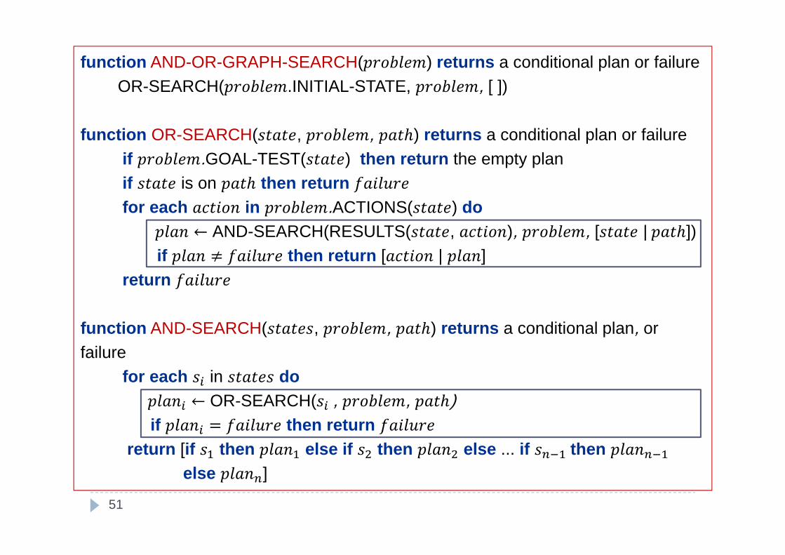
function AND-OR-GRAPH-SEARCH( ) returns a conditional plan or failureOR-SEARCH( .INITIAL-STATE, , [ ])

function OR-SEARCH( , , ℎ) returns a conditional plan or failureif .GOAL-TEST( ) then return the empty plan if is on ℎ then returnfor each in .ACTIONS( ) do← AND-SEARCH(RESULTS( , ), , [ | ℎ])

if ≠ then return [ | ] return

function AND-SEARCH( , , ℎ) returns a conditional plan, or failure

for each in do← OR-SEARCH( , , ℎ) if = then return

return [if then else if then else ... if then else ]

AND-OR-GRAPH-SEARCH

52

Cycles arise often in non-deterministic problems Algorithm returns with failure when the current state is

identical to one of ancestors If there is a non-cyclic path, the earlier consideration of the state is

sufficient Termination is guaranteed in finite state spaces Every path reaches a goal, a dead-end, or a repeated state

Cycles

53

Slippery vacuum world: Left and Right actions sometimesfail (leaving the agent in the same location) No acyclic solution

Suck Right

6

1

2 5

Right

Cycles solution

54

Solution? Cyclic plan: keep on trying an action until it works.

[Suck, : Right, if state = 5 then else Suck] Or equivalently [Suck, while state = 5 do Right, Suck]

What changes are required in thealgorithm to find cyclic solutions? Suck Right

6

1

2 5

Right

Searching with partial observations The agent does not always know its exact state. Agent is in one of several possible states and thus an action

may lead to one of several possible outcomes

Belief state: agent’s current belief about the possiblestates, given the sequence of actions and observations upto that point.

55

Searching with unobservable states(Sensor-less or conformant problem)

56

Initial state: belief = {1, 2, 3, 4, 5, 6, 7, 8}

Action sequence (conformant plan) [Right, Suck, Left, Suck]

Right Suck Left Suck

Belief State Belief state space (instead of physical state space)

It is fully observable Solution is a sequence of actions (even in non-deterministic

environment)

Physical problem: states, , RESULTS ,GOAL_TEST , STEP_COST Sensor-less problem: Up to 2 states, , RESULTS,GOAL_TEST, STEP_COST

57

Sensor-less problem formulation(Belief-state space)

58

States: every possible set of physical states, 2 Initial State: usually the set of all physical states

Actions: ( ) = ⋃ ( )∈ Illegal actions?! i.e., = { , }, ( )≠ ( )

Illegal actions have no effect on the env. (union of physical actions) Illegal actions are not legal at all (intersection of physical actions)


59

S2

S3

S1

S’2

S’3

S’1

S2

S3

S1

S’3S’4

S’1S’2

S’5

Transposition model ( ′ = ( , )) Deterministic actions: ′ = { ′: ′ = ( , ) ∈ } Nondeterministic actions: ′ = ⋃ ( , )∈


60

Transposition model ( ′ = ( , )) Deterministic actions: ′ = { ′: ′ = ( , ) ∈ } Nondeterministic actions: ′ = ⋃ ( , )∈

Goal test: Goal is satisfied when all the physical states in thebelief state satisfy GOAL_TEST .

Step cost: STEP_COST if the cost of an action is the same inall states

2

4

1

3

2

4

1

3

1

3

(b)(a)

Belief-state space for sensor-less deterministic vacuum world

61

Initial state

It is on B &A is clean

It is on A

It is on A &A is clean

Total number of possible belief states? 2 Number of reachable belief states? 12

Sensor-less problem: searching

62

In general, we can use any standard search algorithm.

Searching in these spaces is not usually feasible (scalability) Problem1: No. of reachable belief states

Pruning (subsets or supersets) can reduce this difficulty. Branching factor and solution depth in the belief-state space and

physical state space are not usually such different

Problem2 (main difficulty): No. of physical states in each belief state Using a compact state representation (like formal representation) Incremental belief-state search: Search for solutions by considering

physical states incrementally (not whole belief space) to quickly detectfailure if we reach an unsolvable physical state.


63

Similar to sensor-less, after each action the new beliefstate must be predicted

After each perception the belief state is updated E.g., local sensing vacuum world

After each perception, the belief state can contain at most twophysical states.

We must plan for different possible perceptions


64

= ( , ℎ )_ ( )

Deterministic world

Slippery world

2

4

4

1

2

4

1

3

2

1

3 3

(b)

(a)

4

2

1

3

Right

[A,Dirty]

[B,Dirty]

[B,Clean]

Right[B,Dirty]

[B,Clean]

( )

[ , ]

[ , ]

A position sensor & local dirt sensor

Transition model (partially observable env.)

65

Prediction stage: How does the belief state change after doing an action?= ( , ) Deterministic actions: = { ′: ′ = ( , ) ∈ } Nondeterministic actions: = ⋃ ( , )∈

Possible Perceptions: What are the possible perceptions in a belief state?_ ( ) = { : = ( ) ∈ } Update stage: How is the belief state updated after a perception?( , ) = { : = ( ) ∈ }( , ) = { : = ( , , ) ∈ _ ( ( , )) }

AND-OR search treelocal sensing vacuum world

66

AND-OR search tree on belief states First level

Complete plan[Suck, Right, if Bstate={6} then Suck else []]

= [ , ]

Solving partially observable problems

67

AND-OR graph search

Execute the obtained contingency plan Based on the achieved perception either then-part or else-part

of a condition is run Agent’s belief state is updated when performing actions and

receiving percepts Maintaining the belief state is a core function of any intelligent system

′ = ( , , )

Kindergarten vacuum world exampleBelief state maintenance

68

Local sensing Any square may be dirty at any time

(unless the agent is now cleaning it)

( )= [ , ] ( )= [ , ] ( )= [ , ]7

5

6

2 1

3

6

4

8

2 [B,Dirty]Right[A,Clean]

7

5

Suck

Robot localization example

69

Determining current location given a map of the worldand a sequence of percepts and actions

Perception: one sonar sensor in each direction (tellingobstacle existence) E.g., percepts=NW means there are obstacles to the north and west

Broken navigational system Move action randomly chooses among {Right, Left, Up, Down}

o o o o o o o o o o o o o

o o o o o o

o o o o o o o o o o


70

: o squares

Percept: NSW

= ( , )(red circles)

Execute action = = ( , )

(red circles)


o o o o o o

o o o o o o o o o o



o o o o o o

o o o o o o o o o o


Robot localization example (Cont.)

Robot localization example (Cont.)

71

Percept: NS

= ( , )o o o o o o o o o o o o o

o o o o o o

o o o o o o o o o o


Online search

72

Off-line Search: solution is found before the agent starts actingin the real world

On-line search: interleaves search and acting Necessary in unknown environments Useful in dynamic and semi-dynamic environments Saves computational resource in non-deterministic domains (focusing

only on the contingencies arising during execution) Tradeoff between finding a guaranteed plan (to not get stuck in an undesirable

state during execution) and required time for complete planning ahead

Examples Robot in a new environment must explore to produce a map New born baby Autonomous vehicles

Online search problems Different levels of ignorance

E.g., an explorer robot may not know “laws of physics” about its actions

We assume deterministic & fully observable environment here Also, we assume the agent knows ( ), ( , , ’) that can be

used after knowing ’ as the outcome, _ ( ) Agent must perform an action to determine its outcome

( , ) is found by actually being in and doing

By filling map table, the map of the environment is found.

Agent may access to a heuristic function

73

G

S1

2

3

1 2 3

Competitive ratio

74

Online path cost: total cost of the path that the agentactually travels

Best cost: cost of the shortest path “if it knew the searchspace in advance”

Competitive ratio = Online path cost / Best path cost Smaller values are more desirable

Competitive ratio may be infinite Dead-end state: no goal state is reachable from it

irreversible actions can lead to a dead-end state

Dead-end

75

No algorithm can avoid dead-ends in all state spaces

Simplifying assumption: Safely explorable state space A goal state is achievable from every reachable state

adversary

Algorithms for online search Offline search: node expansion is a simulated process

rather than exerting a real action Can expand a node somewhere in the state space and

immediately expand a node elsewhere

Online search: can discover successors only for thephysical current node Expand nodes in a local order Interleaving search & execution

76

Online search agents

77

Online DFS Physical backtrack (works only for reversible actions)

Goes back to the state from which the agent most recently entered thecurrent state

Works only for state spaces with reversible actions

Online local search: hill-climbing Random walk instead of random restart

Randomly selecting one of available actions (preference to untried actions)

Adding Memory (Learning Real Time A*): more effective To remember and update the costs of all visited nodes.

78

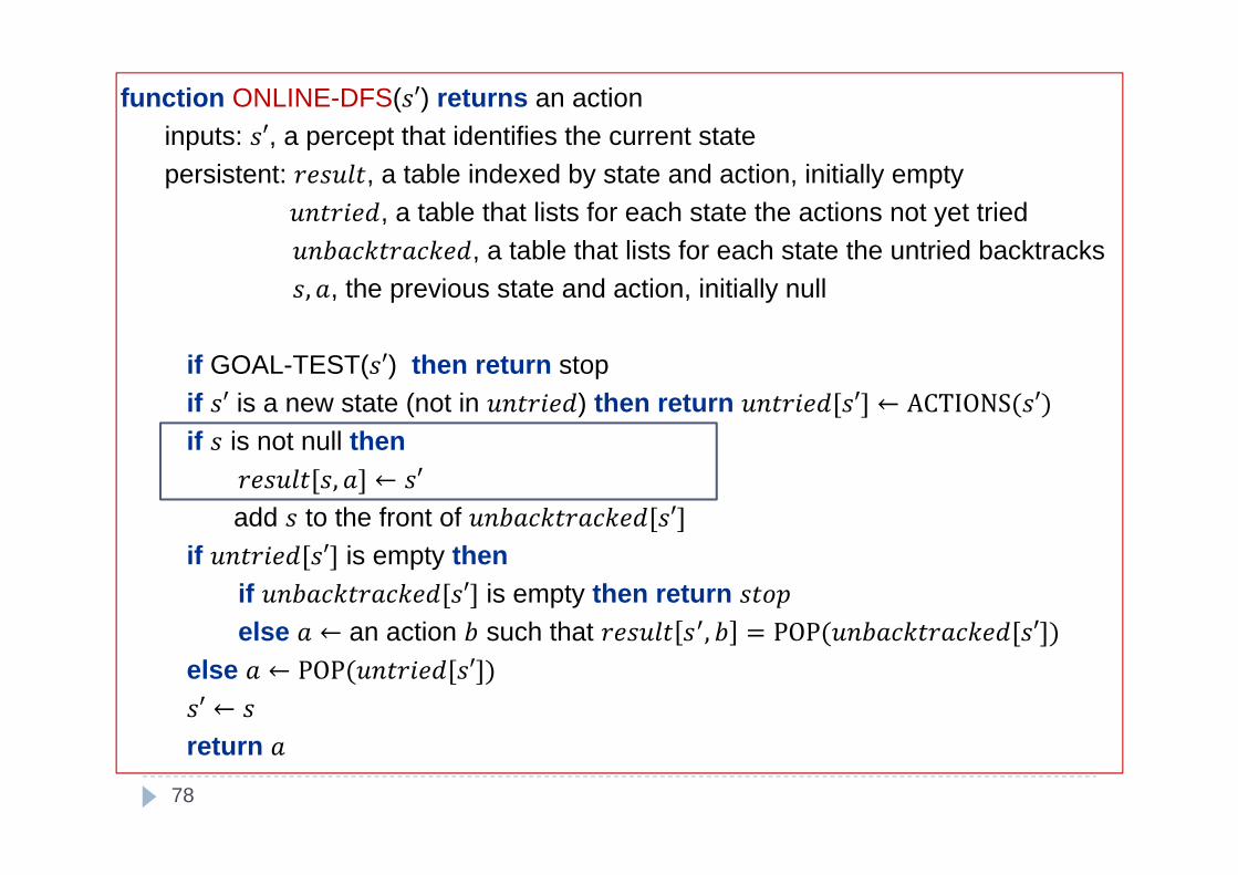
function ONLINE-DFS( ′) returns an actioninputs: ′, a percept that identifies the current statepersistent: , a table indexed by state and action, initially empty

, a table that lists for each state the actions not yet tried, a table that lists for each state the untried backtracks , , the previous state and action, initially null

if GOAL-TEST( ′) then return stop if ′ is a new state (not in ) then return [ ′] ← ACTIONS( ′)if is not null then[ , ] ← ′

add to the front of [ ′]if [ ′] is empty then

if [ ′] is empty then returnelse ← an action such that , = POP( [ ′])

else ← POP( [ ′])′ ←return

LRTA*

79

Following what seems the best path to the goal Best action is selected according to current cost estimates of neighbors

( ):“current best estimate” of the cost to reach the goal Initially ( ) is a heuristic estimate ℎ( ) ( ) is updated by experience (More accurate estimates are acquired using

local updating rules)

Assumption: Untried actions in a state lead to the goal withthe least possible cost ℎ( ) Encouraging to explore new (possibly promising) paths

( )( ) min ( ') ( , , ')a ACTIONS sH s H s c s a s

Learning Real Time A* (LRTA*)

80

function LRTA*( ′) returns an actioninputs: ′, a percept that identifies the current statepersistent: , a table indexed by state and action, initially empty

, a table of cost estimates indexed by state, initially empty , , the previous state and action, initially null

if GOAL-TEST( ′) then return stop if ′ is a new state (not in ) then [ ′] ← ℎ( ′)if is not null then[ , ] ← ′[ ] ← min∈ LRTA∗_COST( , , , , )← an action in ACTIONS ′ that minimizes LRTA∗_COST( ′, , ′, , )′ ←return

function LRTA*_COST( , , , ) returns a cost estimateif ′ is undefined then return ℎ( )else return , , + [ ]

LRTA*: Example (updating cost estimates)

12

1 11 1 11

1 1 11 1 11

1 1 11 1 11

2

2

3

4

4

4

3

3

3

1 1 11 1 113

1 1 11 1 115

3

5

5

4

(a)

(b)

(c)

(d)

(e)

8 9

8

9

8 9

8

9

8 9

44

34

81

ce417: introduction to artificial intelligence sharif...

Documents