ccat mount control using de-convolution for fast...

CCAT mount control using de-convolution for fast scans Peter M. Thompsona, Steve Padinb

asrtems Technology, Inc., Hawthorne, CA, USA, [email protected] California Institute ofTechno.logy, Pasadena, CA USA, [email protected]

ABSTRACT

CCAT will be a 25-meter telescope for submi llimeter wavclcnglh aslronomy located at an altilude of 5600 meters on Cerro Chajnantor in northern Chile. This paper presents an overview of lhe preliminary mount conlrol desi!,'ll. A finite element model of the structure has been developed and is used lo determine lhe dynamics relevanl for mount control. Controller strategies are presented that are designed to meet challenging wind rejection and fast scan requirements. Conventional inner loops are used for encoder-based control. Offset requirements are satisfi ed using innovative command shaping with feedforward and a two-command path structme. The fast scan requirement is satis fied using a new approach based on a de-convolution filler. The de-convolution filter uses an estimate of the c losed loop response obtained from lest signals. Wind jitter requirements remain a challenge and additional sensors such as accelerometers and wind pressure sensors may be needed.

Keywor ds: CCAT, mount control, wind rejection, fast scanning, feed forward, command shaping, de-convolution filter

1. INTRODUCTION

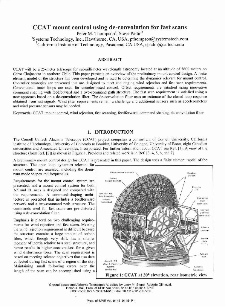
The Cornell Caltech Atacama Telescope (CCAT) project comprises a consortium of Cornell Universi ly, California Tnstitule of Technology, University of Colorado at Boulder, University of Cologne, University of Bonn, eighl Canadian universities and Associated Universities, Tncorporated. For further information about CCAT see Re C [1] . A view of' the structure (from Ref. [2]) is shown in Figure 1. Previous and related work is in Ref. [3, 4, 5, 6, and 71.

A preliminary mount control design for CCAT is !?resented in this paper. The design uses a finite element model of the structure. The open loop dynamics relevant for -r------------- ---------------. mount contro l are assessed, including the dominant mode shapes and frequencies.

Requirements for the mount control system are presented, and a mount control system for both AZ and EL axes is designed and compared with the requirements. A command-shaping architecture is presented that includes a feedforward network and a two-command path structure. The commands used for fast scans are pre-distorted using a de-convolution filte r.

E mphasis is placed on two challenging requirements for wind rejection and fast scans. Meeling the wind rejection requirement is di fficull because the structure contains a large amount of carbon fiber, which though very sti rr: has a smaller moment of inertia re lative to a steel structure, and hence results in higher accelerations for a given wind disturbance force. The scan requirement is based on meeting science objectives that use data collected during fast scans of a region of the sky. Maintaining smal I fo llowing errors over the length of the scan can be accomplished using a

!-Jnmo.ry i:;.uppnrt ~m1rturn

t.y!'..t('f'h'I.

(boll\ &fl.It-$)

l\::r trn uih HSB. tJJ ivt: & t:nLotfCI

svsteni)

(both .;d.,)

Nasmyt.h

p1.otforms

(both ~hfo.\ )

! Atirnuth

S!flJCIU fC

Alimu1h

pin tie

Atin1uth 1rw·l

, Cnnt r,_t,.,

fotJndo t;oo

Figure l : CCA T at 20° elevation, rear isometric view

Ground-based and Airborne Telescopes V, edited by Larry M. Stepp, Roberto Gilmozzi, Helen J . Hall , Proc. of SPIE Vol. 9145, 91451P•©2014 SPIE

CCC code: 0277-786X/14/$18 • doi: 10.1117/12.2057250

Proc. of SPIE Vol. 9145 91451P-1

de-convolution filler, which distorts the input AZ and EL scan patterns so that the on-the-sky path meets lhe requirements.

In the mount control design effort the principle was fo llowed where the controller fo llows from a good understandin g of the "controlled clement." This understanding is included in Ref. [3] and is summarized here in Section 2. The w ind model assumes fully developed, von Karman turbulence on the M2 and M 1 structures. Section 3 describes the wind mode l. T he parameter values arc lis ted in Table I. The mount control design is presented in Section 4 sta rling with req uirements. The feedback archi tecture and the various fillers are each discussed. Closed loop ana lysis is presented in Section 5, inc luding stability analysis, nodding performance, and wind jitter.

The requirement for fast scanning over a region of the sky is a performance requirement lhal distinguishes submillimctcr wavelength te lescopes from optical te lescopes. Section 6 explains why this is hard to do, present a method for meeting the requirement, and then shows by example that the me thod called "de-convolution" is feasib le.

Conclusions of this study and next steps are presented in Section 7.

2. STRUCTURAL MODEL

A finite element model ofCCAT was developed by SG H (Rerf2]). The full order model was developed using ANSYS, with different versions of the model available al 90 and 20 degrees e levation. The complete ANSYS model is very important for the mechanical desig n of the structure, but due lo the large size of the model it is inefficient to use for mount control design. For this reason a reduced order model was created that matches the frequency response of the full order model al selected nodes up to 50 Hz. The nodes that arc primarily of interest are at the mount control force input local ions, encoder locations, and locations on the M 1 and M2 struc tures that can be used to approximate wind disturbance forces. Additional nodes were also selected lo provide a good visualization of the low frequency, large spatial reso lution structural modes. The model reduction was done within ANSYS, resulting in a model with 674 modes and 54 nodes, with 6 degrees of freedom at each node. The data for thi s model is stored in a text file that can be loaded into Matlab for analys is and design.

A choice needs to be made on how the include lhe AZ and EL-axis drives in the reduced order model. The best approach is to release the rotary motion for both drives so that both are free lo move. Technically this means there arc structural modes al 0 I lz for each drive. lf for numerical reasons a s tructural mode at zero cannot be handled, inc lude a very soil rotary spring on each axis. Just to be clear, do not constrain or include a stiff spring on one axis and free up the other. Free up both axes. Constra in or include a sli ff spring i r desired after creating the reduced order model with both axes free. An advantage of freeing up both axes is the same model can be used for bolh AZ and EL mount control design.

2.1 EL-Axis Survey

T he open loop and locked rotor EL-axis responses arc surveyed in Figure 2, where:

• EL is from the motor torque input lo the encoder output • M2 is the response of torque applied al M2 lo the angular change at M2 • MI is tip-Zcmike torque applied at M I lo the tip-Zcrnikc angular response at M I

The frequency responses include both the E20 and E90 cases (20 and 90 degrees e levation). T he responses are nol significantly different; from which it can be inferred that a controller without gain changes can be used over this range of elevat ion angles. The Ml and M2 responses are locked rotor responses, which are included because I.hey arc used to dete rmine the best possible w ind r~j ection. Any response thal is " locked" is flat. at low frequency, and the resul ting s teady state compliance is marked on the fi gures. The locked rotor zeroes for E20 and E90 respectively at 5.79 and 5.96 in the EL responses "flip over" when the EL-axis is locked to become poles al the same frequencies in the M2 response and near-the-same frequenc ies in the MI response.

Structural mode shape diagrams at 9.6 and 11 .2 I lz are included in Figure 2, which correspond to peaks at (a lmost) the same frequencies in the EL response. The M I and M2 structures move differentially at 9.5 Hz and together at 11 .1 I lz. The so-called " dine rentia l resonance" at 9.5 Hz imposes a limit on performance. This happens indirectly because a s tructural filler is needed to reduce the gain a t the differential resonance, which can on ly be done by introducing phase lag, which in turn makes it necessary to change the PIO gains lo introduce more phase lead, which results in lower gain al low frequency, and hence results in lower wind rejection.

Proc. of SPIE Vol. 9145 91451 P-2

'O

! •. !0.257 !mosiN-ml

10. f·

~ i

10 '·)t

[ 10 "l

..Ir::==:·~~ 10 l .•. . . '

10·

10 i !

10 'i

5 79 5.9S

10'

Frequency (Hz)

10 Froquoncy (Hz)

EL

M2

1 ~ ·10 -10

30 .

is· 11 .2 Hz

10 20

M1 j 1 1

15

10

I 0 -

1 J l

- . ~I 10'

Figu re 2: Open loop EL-axis survey

The EL-axis response has a fore-alt-sway mode al 3.84 H z where lhe AZ and EL structure move togelher as a rigid body relative lo lhe pier. The sway mode is almost cancel ed by the nearby and slightly lower frequency zero at 3. 76 Hz, which means this mode can be ignored in the mount control design.

In the mode shape diagrams, the rectangle c lose to the botlom of the MI truss represents the EL-axis tube, and the plus at the top of the AZ-slruclure is the middle location of lhe EL-axis drive. The lines on the mode shape diagram connecl the nodes selected for lhe reduced order model, and roughly but not exactly correspond to slruclural members. The "full" mode shape with thousands of I ines is available using AN SYS and were used to help understand lhe slrnclure. The reduced order mode shapes were also used, and arguably are sometimes better at helping to understand relative motion. ln any case, to emphasize to design approach actually used, the reduced order mode shape diagrams are included here.

All of the EL-axis responses depend (weakly but a little bit) on whelher or not the AZ-axis is closed, and vice-versa. In all o f the responses shown in Figure 2 and f igure 3 the drive on the opposite axis is open.


10

J • 3 •2o7 [<g·m'J !EllO) AZ J • 3 39o7 fl<g·m' )(E20t 4.83 Hz

•o 20

i 1(1 15 •ae

~ • 862 10 7 11

;\. fl \.' ~ 10

468 \ " ~ /·!·' 10 J, •.

~ ' ., " 'I ~r , \)\ q. I t; \

5 10 ·Ii I &01 \ \ 1

E90J 8.87 \

E20 102

10 . ~ 0

'° 10 1(\

F1tque"'cy {Hz.J

10

AZM2 10

8}3 II

10 J\ 10.7

/ I ~ • 63 s.es \ ·

_ o 238 (mas/N·m) ~ • ' 1 ,, f 10 596 l/ ·, I .10 •es \i \. \ ~ ~ 0 .5

~ " I . . \ 10 5

9.12 ~ V1 \ /V \. ., \1 I I/ '· I' 10 I JI \ \

10

10 L@l

10 10 ·o' Frequoncy (Hz)

·o AZM1

~ 0

IC

8 23

I I

" f ,. ~ 10

; !~

!; 463 HS ¥ ,1

0 044 (mHIN·Ml 5 94

~~<I 10

47 ' •o

... 'l 10 4

'1 \ , i '

_J

[ I:-@ I I~ 10 10 .15 H 1i <I

10 10 '0 1n'

F19q.,.nc:y (Hzj

Figure 3: Open loop AZ-axis survey

2.2 AZ-Axis Survey

A simi lar open loop AZ-axis survey is in Fig ure 3, where:

• AZ is from the motor torque input lo the encoder output • AZM2 is the response from torque applied at M2 to the angul ar change al M2 with the AZ-axis locked • /\ZMl is ti lt-Zernikc torque applied at M 1 lo the tile-Zernikc angular response at M 1 with the AZ-ax is locked

The moment-of-ine1iia about the AZ-axis for E20 and E90 changes less than one percent, but there is a significant change in the locked rotor zero (respectively 8.0 I to 8.87 Hz) and the differential resonance (respectively 8.62 to I 0. 7 Hz). T he same gains are used in the AZ-axis mount control despite these changes, but a gain schedule will be considered during the detailed design phase. The AZ and EL-structures move together for the mode shape at 4.83 Hz, and differentially for the mode shape at I 0.7 Hz. The former is not a factor in the AZ-ax is mount control, and the laller limits the AZ-axis bandwidth .


2.3 The Softening Effect of the AZ-Structure

If the EL-structure is mounted on a rigid base and the EL-axis rotor is locked, the dominant frequency of the ELstructure is l0.1 Hz. This is the frequency, and corresponding stiffness, to which the EL-structure was designed. The expectation was the locked rotor zero for the EL-ax is drive response would be at I 0.1 Hz, or something close. The rigid base locked rotor freq uency response at M2 is shown in Figure 4 and should be compared with the M2 response in Figure 2, mounted on the AZ-structure.

101

M2

Frequency (Hz)

Figure 4: M2 response of EL-structure mounted on a rigid base

The dominant frequency has dropped 41 % from 10.1 to 5.96 Hz (at E90), and the rotary compliance at M2 has increased 84% from 0.14 mas/N-m to 0.257 mas/N -111 (milli-arc-second per Newton-meter). This is the softening effect of mounting on the AZ-structure. This effecl is examined in more detail in Ref (3]. There is no "weak link" in the AZstructure; the compliance is distributed more-or-less evenly from the hydrostatic bearings at the top of the AZ-structure lo the movement of the pier in the ground. This means stiffening any one part of the AZ-structure or pier will not make up the difl"erence. Nevertheless, limited improvements are being considered.

3. WIND MODEL

The di stributed wind force on the EL-structure results in torques about both the EL and AZ-axes. The steady state wind force is countered by steady state EL and AZ-axis drive motor torque, which is one part of the calculatio n for required motor torque. The wind turbulence results in stochastic pointing error. The wind turbulence is approx imated using a von Karman spectrum, injected into the system as four different: distw-bance inputs: M l and M2, AZ and EL. The parameter estimates for the von Karman spectrum are li sted in Table I.

3.1 Dist·urbaoce inputs

Define an EL-structure Cartesian coordinate system where the EL-axis rolates about the x-axis, the z-axis is positi ve up, and the y-axis is the right-hand complement.

M2 EL-Axis: The wind is a point force in the y-axis direction, perpendicular to the EL-axis of rotation, with an nns value of F, applied at a single node on the M2 structure a distance Ru2 from the EL-axis of rotation. The resulting torque about the EL-axis is TF.I,ui. = FRu2.

M2 AZ-Axis: The wind is a point force in the x-axis direction, perpendicular to the AZ-ax is of rotation, with an rms value ofF, applied at the same node on the M2 structure, w ith a lever arm of R,w2cos(EL). The resulting torque about the AZ-ax is is T;1zM2 = FR,112cos(EL). When the telescope is pointing at Zenith the elevation angle is EL=90 deg and there is no wind torque about the AZ-axis.

Ml EL-Axis: The total wind force in the z-axis direction is assumed to be uniformly distributed on one-half of M J, divided in half by the y-axis, resulting in a torq ue about the EL-axis. Call this the tip direction. This is equivalent to assuming half of the force is in opposite directions on either side of M J. The torque about the EL-axis is TnMi = /,ydF = FR«ff• where the effective radius of Ml works out to be R~rr = (4/(3n))RM1 "" 0.424RM1 and where RM1 is the actual radius o f Ml. Tn the reduced order finite element model, the total force is distributed about the ava ilable nodes on the M l structure as described in Ref. [3].


Ml AZ-Axis: ln a similar way the total wind force in the z-axis direction is assumed to be uniformly distributed on onehal r or M 1 as divided by the x-axis. Call this the tilt direction. The resulting torque about the AZ-axis is TAZMI =

cos(EL)FR~1r-

3.2 von Karman Spectrum

The wind force on a structure due to turbulence is assumed to sati sfy the fol lowing von Karman sp ectra:

<IJ(f') = F2 (O. 77 I Io) . [1+ (/ / .f(J)2]716

Where the rms w ind force is:

The external w ind speed of Ucj) is decreased to U = JL Ucj) al the M2 and M 1 structures. The parameter pis the density of a ir, C0 is the drag coefficient, A is the area or the s tructure, and dis a de-correlation coefficient. The von Karman break frequency is .fo = UID where D is the characteristic length or the turbulence, equal to the dome opening. The VOil Karman parameters used for the M2 and MI structures are listed in Table 1. The turbulence mode l is assumed to be the same in each of the x, y, and z directions.

Table 1: Wind Model Paramet'crs Parameter Definition M2 Ml

Independent parameters

u<XI [m/sec] 90'11 percentile external wind 9 9 speed

J1 [unit less] Wind speed reduction factor 0.4 0.2

p [kg/m 3] Density of air 0.7 0. 7

cf) [unitless] Drag coefficient 1 I

D rm] Characteristic length (equal 30 30 to dome opening)

d [unitless] Decorrelation factor 1 (worst case) l (worst case)

A [m2] Area of the structure 9 245 (1/2 ofM I)

Calculated parameters

U [m/sec] 90'11 percentile wind speed at 3.6 1.8 the structure

p [N] rms force 40.8 278

lo [T-fr.) von Karman break frequency 0.12 0.06

3.3 Decorrelation

M2 Structure: Decorrelation occurs due to vortex shedding that changes the von Karman spectrum so there is more energy at high frequency. This shift tends to reduce the rrns response and is included in the model by using a decorrelation factor d < l. This effect is considered small (perhaps I 0%) and the worst case va lued= 1 is used for M2 wind analysis.

Ml Structure: The worst case decorrelation of d = 1 assumes all of the available force is applied in either the tip or tilt direction. In reality only a portion is appl ied in tip and tilt. Some of the force, for example, is uniform across Ml, which does not result in torque about either axis. A reasonable assumption for the distribution of the total force is divide the variance among Zernikes, with 'f.t of the variance in the piston direction, '/, in the tip direction, '/. in the t ilt direction, and the remaining '/, di stributed among the higher order Zernikes [Ref 8]. The decorrelation coefficient is applied to therms force, and so would be d = sqrt('/.) = Yi in each of the tip and tilt directions. In this way the wind force and he nce the torque on M I can be reduced from the worst case assumption of cl = I.


4. MOUNT CONTROL DESIGN

4.1 Requirements

Performance requirements based on science objectives flow down to the following set of qualitative and quantitative requirements used for the control system design:

• Maximize wind r~jection (by maximizing low-frequency loop gain) • Acceptable robustness (phase margin > 30 deg, gain margin > 6 dB) • Structural peaks gain stabilized (peaks magnitudes - 6 dB) • Use feed forward lo improve nodding performance • Shape the pointing conunands with velocity and acceleration limits

Drive parameters are listed in Table 2 (Table I from Re L [4]). N umerical requirements for nodding, wind jitter and scanning are introduced in the sections where the results of the preliminary design are analyzed.

4.2 Feedback Architecture

The mount control architecture in Figure S was used for the preliminary design. T he on ly sensors arc the encoders. The heart of the controller in Figure Sa is a Proportional-Integral-Derivative (PID) compensator with a structural filler. The diagram shows disturbance inputs for wind, torque ripple, and encoder quantization . The axis rotations at the M I and M2 locations are used lo estimate wind jiller and scanning performance. These rotations are simi lar lo (but not quite the same as) line-of-sight variations computed using ray-tracing on distorted structures.

A choice needs to be made to use just position feedback or both velocity and position. The velocity is derived from the same encoder. Separate velocity and position loops are shown in Figure Sb and is the preferred architecture going forward. Both architectures are the same in regards to the disturbance responses, but the command response differs. The two loop structure is preferred because it provides more lag in the command path and hence results in less structura l vibration, and because it results in a feedforward design that is less sensitive to parameter changes in the structure.

Both one and two path versions of the command shaper are shown respectively in Figure Sb and c. The one-path version is the usual approach. Offsets are on-the-sky and injected before the pointing model. The two-path version preserves the on-the-sky offsets with improved transient response. The commands from the pointing model pass through one or two minimum time command shapers which limit both the velocity and acceleration. The velocity limit is based on avai lable braking and the acceleration limi t on the avai lable power. T he command shaper has worked successfully on Keck and is recommended for use on CCAT. The shaped command is passed through high order low pass filler that limits the jerk. The feedforward network, which must be properly tuned, results in small moves with less overshoot and faster settling. Further detai ls on the two-path version are in Ref. [71.

4.3 PID Design

The three gains of the PID controller are computed as funct ions of three design parameters. The design parameters are exactly achieved for a rigid body system, and close enough otherwise. The design parameters are:

.fc. [Hz] = unit magnitude crossover freq uency PM [deg] = phase margin LGM [dB] = lower gain margin

The phase margin is extra phase lag that destabilizes the system, and the lower gain margin is the gain reduction that destabilizes the system. Jt fo llows non-obviously that:

2 LGM/20 k; = -flm~ /( lgrnxsqrt(l + /12

)) {fl = tan(90+ PM)

kp = fl(k; - % )/ % where lgrn = 10

k,. = lgm xJxk; I kp % = 2nfc

( I )

The rate gain varies with the moment of inertia J and hence is a very large number. The other gains end up being modest sized numbers. This method is from Ref. [6]. Disturbance rejection is increased by increasing .fc., decreasing PM and decreasing LGM. Robustness is increased by going the other way. The goal is to move./;. closer of the locked rotor zero. Within SO% would be very good, and about 40% is achieved.


Table 2: Drive Parameters

P arameter AZ EL l',···-1 ' /" t".f) J S X A ,1 .J /Hll 1 ° -·1 ' /'\r(l (, S X A , •) /till

Scan an:c•lf'rat ion IO -'> , /''~() J s - x "· ,,.. /llll j "s - 2 x ,.\ / 3.'.iO 1rn1

Slew sp('('d

Slew acceleration

J<>s l

2'\i-'..'

3 05-l

2°s -'..'

Axis inertia 2.G >'. 107 kg m 2 2.6 x 10" kg 111:!

i\1otor radius

'forqnc for slew acc0lernt iou

Avai lable muLOr Lorquc

9 . 1

1.1

9.5 Ill

x 10" Nm X !OH :\11t1

·1 Ill

!) .1 x '104 Nill 1.8 x 10-:, Nm

G(s) EL

Servo Structura l fil ter CCAT

Encoder s ignal

a) PIO and structural filler (shown for EL-axis, s imilar for AZ-axis)

[AZ] [

Ra J [ Ra J EL totol Dec Dec total ~--~

___ 1_"'-"'--..~ J----t~ Pointing 1----t~I Model

M inimum T ime Jerk filter Command Slwp~r

.f.·rr = sg~),, where !:,·cl'" ...!!:!.EL and w .. t7.

. Tm.'-"'"' T.~Jlm,d

l Ra J llcc

o11Sc1 [AL] El "' 1.;l lC

Pointing ( I command path) Mount Contro l

b) Pointing, command shaping, and feedfoward (I path)

[6~~] l~i'J ___ 1_1a_sc~---...i Pointing 1---~-----l_m_~ ... ·-~

Model

Pointing 1---~1

Model

Po inting (2 coinmand p:1tlts )

[AZ] EL ~ olTM:t

c) 2 path version

[AZ] EL ' c111d

Mount Control

Figure S: Mount contrnl feedback architectu re


[AZ] EL enc

[TAzl 7" /•./, ·111d

[wAz J rolil enc

[(""z] fr> '

''·'~ cmd

4.4 Structural Filter Design

The structural filter gain stabi lizes the structural modes by reducing a ll of the peaks to -6 dB or lower. The filter is a series of lags and/or notches with a de gain of one. There is a difficult tradeolf in the structural filter design between a potentially large amount gain reduction (for gain stability) and a small amount of phase lag (for better performance). The following filter called a "staggered notch" worked well for the preliminary design:

2 f(s) = (s / co11 )

2 +2S-11 (s l rv11 ) +1

(s l i»J) +2sd(s l rvt1)+l

Place the pole frequency al cod rad/sec near the locked rotor zero and the zero at rv,, near the differential resonance. This "stagger" in frequencies results in significant gain reduction. further reduce the ga in at the differential resonance by setting the numerator damping ratio (,, to 0.2 or lower. Values less than about 0.05 are not desired because the design becomes sensitive to the exact location of the differential resonance. The denominator damping ratio of (c1 = 0. 5 provides a good balance with low phase lag without a s ignificant change in gain near the locked rotor zero. f urther lags al higher frequency are good design practice. Adjustments in the structural tilter will like ly be needed as the model matures and then again when the response of the actual structure is measured. The goal is to use one set o f constant parameters for each axis, each set of parameters good for all elevation angles.

4.5 Feedforward Design

The feedforward network inverts the closed velocity loop response and idea lly is a pure velocity feedforward, which in Laplace notation is j{s) = s. Jn practice the velocity loop has lag which must also be inverted using lead, and a filter is recommended of the form ./{s) = s(as2 + bs + I). The parameters of the feed forward network can be estimated from the finite element model and eventually from measurements. The feedforward tilter is implemented in combination with the j erk filter. The jerk filter must be higher than third order lo prevent the implementation of potentially noisy derivatives. The details are in Ref. [3]. Tuning is important. Stability is not a problem, but mismatches result in overshoot, the reduction of which is the goal.

4.6 Jerk Filter Design

Step changes in acceleration are prevented using a linear lime invariant filter called a jerk filter. For the one-path command shaper the jerk filter must have zero velocity error (called fia82). Technically, ifta82 - 1 )/s = 0 as s~O. For the two-path solution, better offset performance is obtained by passing the offset portion through a zero position error filter (calledfia8 1). Sixth order tilters were used as shown below:

I ( • s /0111 + 5-r f ast )s + 1 ftag 1 (s) = 6' ftag2 (s) = 5

(r: fasts+ 1) ( • s/mvS +I)(• /asls +I)

Time constants using in the preliminary design are l /(2tr1j;,,1) = 8 Hz and l /(2n-r,1o.,,) = 0.331-lz.

5. MOUNT CONTROL ANALYSIS

5.1 Stability Analysis

The controller gains are not included here but the resulting loop trans fer function s are shown in Figure 6. T he " loop transfer function" is the frequency response or the open loop system response times the controller ti lters. This is the response that is shaped by the controller design. The design objectives are to maximize both the crossover frequency fc and the low frequency gain, with the limitation of keeping the structural peaks all below - 6 dB. The achieved crossover frequencies for the EL and AZ-axes are respectively 2. 5 and 2.9 Hz, respectively 40% and 36% of the locked rotor zeroes at 6 and 8 Hz. The highest structura l peak is about - 5 dB. The phase margins (PM) arc well above 30 degrees. The delay margins (DM) are noted in the figure and are the added delay tha t destabilizes. ln both loops the sway mode is "phase stabilized," which means the phase blips due to these modes increase and hence are not a stability problem. The design is considered aggressive, which can be made even more so by lowering the phase margin.


40

Differen~al EL-ltf Differential

le= 2.9 Hz 4 AZ-itf' ·1

/ . Maximtze gain Cil 20 I' ~ :; Maximize gain . / E20 peaks above -6 dB

~ 0 le = 2.5H ~ E • ·-,.;. • r . ~ ( -6 dB I - -6dB

gi :t \to~ ·- -· '1\ '..J·v1 f;· ""' '._,'-" .... :i: -20~ / \• ,1 I) .

I_ E20 I Sway ·~ 188 - .:. - - .;_:_:......:.----------~--~-~-~-~- ~-:

90

0

5: -90

"' ff. -1801

270.

·3601, 10

.r t I·.' ,,, . 1: )~• , ( - ,\.;\)" ... vi ... '""·" ''-. ..

..... ) .. A) F>M~46de9 .

OM ~ 44.6 msec

Frequency (Hz)

~ 9~'l; :!;!. " -90

~ -1 80

·2l 0

·350 10

1

Figure 6: Stability Analysis

5.2 Nodding Analysis

' r 1\

/ \,,, .. .,.\ \ f1\ . " '"•

Sway · \/ \I .. 1 / ...; '---

~~~--- _ .. Y! .w J

1..l

" 10

./1 "./ ... "i \ r··1 . t' ~· . .. ,,.. ) .

, lj Ii 't - . ~ !\' ,~ PM= 50 deg - ·'·

OM= 48.2 msec

Frequency (Hz)

The requirement for a one degree nod is to settle within one-tenth beam in 3 seconds. For bearnwidths of A.= I 000 and 350 microns this translates to setlling error less than » I 000 = 1.00 and 0.35 ArcSec. The two-path command shaper in Figure Sc is needed to meet the 3 second requirement. A p lot of the si mulation results is not included here, but the achieved settling times are listed below:

Error< 1.00 ArcSec , EL = 1 . 72 [sec] , AZ=2 . 22 [sec] Error < 0 . 35 ArcSec , EL = 2 . 52 [sec ], AZ=2 . 78 [sec]

For smaller moves the nodding requirement is stated using number of beamwidths, with the settling time bei ng the time for the response to stay wi thin I/10th beamwidth. The 350 micron results are reported here. S imulation results are plolled in Figure 7 for nods of 3, 5, I 0, and 20 beamwidths. The settling times are listed below:

yLarget = 3 ytarget = 5 ytarget= 10 y target= 20

[beamwidths] [beamwidths] [beamwidths] [beamwidths]

(10.5 [ArcSec]), EL (17 . 5 [ArcSec]) , EL (35 . 0 [ArcSec]) , EL (70 . 0 [ArcSec]), EL

so~-~--~-~--~---,--,----,

70

J 60 r I , I 50 ; ;

'° ry. 30 /1'

--·- - ·-- .. -- ......... ,_. ___ _

u Ql (/)

~ ro

10

8

6

4

2 -

0

-2

-4

-6

1. 23 [sec], AZ=l. 21 [sec ] 1 . 52 [sec] , AZ= l . 45 [sec ] 1 . 81 [sec], AZ= l . 72 [sec ] 2 . 12 [sec], AZ=2 . 10 [sec]

:: [ ;-=: :~~~~ _ ---= ~ - Shaped command !J - - EL Response

0 i

1 , AZ Response

-8

1

- ELError I -- AZ Error

:!c 1/10lh beamwidth (0.35 arcsec)

0 0.5 1.5 2 ~5 3 15 4 -10

0 1.5 2 2.5 3 3.5 4 Seconds Seconds

Figure 7: Nodding Analysis (350 micron bandwidth)

Proc. ofSPIE Vol. 9145 91451P-10

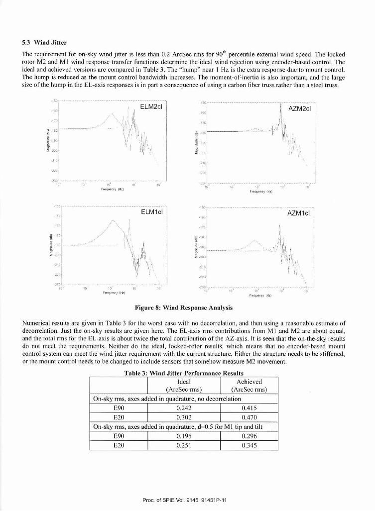
5.3 Wind Jitter

The requirement for on-sky wind jitter is Jess than 0.2 ArcSec rms for 90111 percentile external wind speed. The locked rotor M2 and MI wind response transfer functions determine the ideal wind rejection using encoder-based control. The ideal and achieved versions are compared in Table 3 . The "hump" near l Hz is the extra response due to mount contro l. The hump is reduced as the mount control bandwidth increases. The moment-of-inertia is a lso important, and the large size oftbe hump in the EL-axis responses is in part a consequence of using a carbon fiber truss rather than a steel truss.

. 1 :o

·?.30 , 11)

·!~O-

- 1~1)

· 1'0

-:?'lO· I

220f

.no 1•

10'

IO

10

ELM2cl I I ,-, l ·i

·. ' 1 ',·<'t 1j.11 . "f ft I, J . 'tl l v · ·r.tu

d · 1:1 .!

' hi'·/ l l

' i Q 10

Frequi=ncy (H.t)

ELM1cl

10' 10° 10: Frequency (H.t)

.J70·

10'

Figure 8: Wind Response AnaJysis

10' 101

FreQUbl\C)' !Ht)

AZM1cl

1</ 101

10·

F'r•quotle~ (Hz.)

Numerical results are given in Table 3 for the worst case with no decorrelation, and then using a reasonable estimate of decorrelation. Just the on-sky resul ts are given here. The EL-ax is rms contributions from MI and M2 are about equal, and the total rms for the EL-ax is is about twice the total contribution of the AZ-ax is. It is seen that the on-the-sky results do not meet the requirements. Neither do the ideal, locked-rotor results, which means that no encoder-based mount control system can meet the wind jitter requirement with the current structure. Either the structure needs to be stiffened, or the mount control needs lo be changed to include sensors that somehow measure M2 movement.

Table 3: Wind Jitter Performance Results Ideal Achieved

(ArcSec rms) (ArcSec rms)

On-sky rms, axes added in quadrature, no decorrelation

E90 0.242 0.41 5

E20 0.302 0.470

On-sky rms, axes added in quadrature, d=0.5 for Ml tip and tilt

E90 0.195 0.296

E20 0.251 0.345


6. FAST SCAN PERFORMANCE

An important requirement is to scan a region o r the sky uniformly to minimize image artifacts. CCAT w ill u se Lissajous patterns, and simi lar continuous scans, with no blanking during turn-arounds. Simp le versions o r the Lissajous scan pa tterns were used for the pre liminary design, with the max imum ve locity and acceleration o f the scan equa l to the maximum available velocity and accele rat ion. The error used to assure no missed segments du ring the scan is one -half beamwidth, which is A.1200 = 1.75 ArcSec fo r a A, = 350 micron beam width.

To start the analysis, consider a sinusoidal scan in just one axis, with s imulat ion results shown in Figure 9. ft is seen that the e rror far exceeds 1. 75 ArcSec. Why did this happen? Mount control systems are desig ned for zero position erro r !o r constant ve loc ity inputs. Standard mount control systems work for raster scans because each scan line is (not quite but very nearly) a constant velocity input. The sinusoidal input, and more gene rally Lissajous scan patterns, are nowhere close to being constant ve loc ity.

011

0.081 !

:::1·.;· " 0.02[,

fil' 0 .,, -002 !

-0.04

-006

-0.08

-0 10 2

\ \ \

·-···· ] ,I :I

,·

1

i.,,, -;;;~~co~;JI 4 6 8 10 Seconds

a) Response

60

" (\ /\ ,/\\ 1. ! \ . l

20 ' , \ ; \ .,

f \ 1 I \ J

~ 01 i \ ! \ I \ Ii

-20 f \ // \ I \ ;JI I \ I ! I i

-401 ' \ \j \/ : -60 l --~-· -- ~- -- -•·--·J=~~=-~!~?r Jj

o 2 4 s a 10 Seconds

b) Error

Figu re 9: Sinusoidal scan in one axis

The proposed approach is to pre-distort the scan commands so that the achieved on-the-sky pattern is the desired pat1ern. T his method is demonstrated for sinusoidal inputs in F igure 10. The response of a linear system to inp ut u(t) = A sin( ax) is y(t) = A Rs in( ux + ¢), where g(j cv) = Rexp(j</J) is the response of the system at the input frequency. Use the pre-distorted input ii (t) = (AIR) sin( ux - ¢). T he Lissajous pattern in Figure 10a is a sinusoid in each axis. The error response in Fig ure 1 Ob is without pre-distortion and in Figure 1 Oc atler p re-distortion. 1l takes about 3 seconds for the error to settle, but then setlles to well less than the required value or 1.75 ArcSec.

0.1

0.08

0.06 .

0.04

Ol 0.02 .

(l)

2. 0 ...J w

-0.02

-0.04

-0 06

-0.08

-0.1 -0.4

aol1! 60. !

:i; ! ~ 401r\ ! "' ,,

2oi V i

o! 0

RMS Error (no input correction )

;\(\! \( \Ir\/ v v· v ~ v

L •'l. J

.. / \

\ \ r \I

v 5 10 15 20

b) Error wi th no inn ut correction . ' ...... .... "]

RMS Error (after input correct:on) J

1 75ArcSec ~

· 0.3 -0.2 -0.1 0 0.1 0.2 0.3 0.4 -.1 -.--.. -15 20 AZ [deg] Seconds

a) Response b) Error a fter input conection

Figure 10: 350 micron Lissa.jous Scan

Proc. of SPIE Vol.. 9145 91451P-12

The gain of the system at the input frequency needs to be known lo a high degree of accuracy. Define R as the assumed gain and define R + £as the actual gain. Using trigonometric identities, it works out th al the steady slale error wi 11 be less than the required va lue of E if the gain error is& < EIA. Tn lhe Figure I 0 example, E = 1.75 ArcSec, A = 300 ArcSec, and the gain error works out to be less lhan about 112 percent.

The pre-distortion scheme used in Figure 10 shows promise but is not sufficient. Constant gain sinusoids, or more generally a constant gain Fourier series, is not sufficient for a region-filling Lissajous pattern. There are two problems with the example in Figure J 0, the settling time is too long and more importantly, the gain of lhe input signal cannot be constant. A pre-distortion scheme based on the steady state frequency response is therefore nol sufficient.

The recommended approach is called "de-convolulion." Define u(t) as the desired axis command, g(t) as the impulse response of the closed loop system, and then lhe encoder response y(I) is the convolution:

y (t) = J 1 g( r )u(t - r)dr

'o

The sampled vers ion of lhe convolution can be wrilten as lhe matrix product y = Ug, where U is a matrix with the samples of u along diagonals and sub-diagonals. The impul se response is eslimated using de-convolution:

g=U+y

Where u+ is lhe pseudo-inverse. The estimated impulse response is used to build another banded matrix G. The distorted input that achieves y = u is computed using a second de-convolution:

-+ u=G u

So there are actual ly two de-convolutions, one to estimate the impulse response, and a second to create the di sto1ted input. A nice fealme of working with impulse responses is number of degrees of freedom does not need to be known. The de-convolution method is demonslrated in Figure 11. The example uses a structure with 676 dof.

Cl Q) "'O

1 (\~).. o.5 /AZ I \ /.,,

I I \ I \ t/ \ / \\ II \ \ / \ ;!' \ \ / \

o· \ ,1 \ \ , " '\' \ \j\ \,1 \/.\ \/ \/ \) EL- - I - - - ·-!

I I \ / I ~' . -0.5

. j -1 ~~~~~~~~~~~~~~~~

03

0.25

0.2

0 5 10 Seconds

;j

15

,/~ Deconvolved AZ /fk"

/_,' ··7"

/,/ g> 015 "'O I

.' / r

,... ../ ..... -) ... .,/ ,-' "'-

0.05 ,/ ' ""'

0. /,/ Deconvolved EL

0.1

0 0.1 0.2 0.3 0 4 0.5 0.6

Seconds

-0.4 -1 -0.5 0

AZ [deg] 10

8

(..) Q)

6 (/) (..) 4 -'-ro

2-RMS ERROR

0 !W,.~ ........ _ _ ..... ___ ~

0 5 10 Seconds

Figure 11: De-convolu tion example for a 1000 micron Lissajous scan


0.5 1

5ArcSec

15

The scan pattern is a sinusoid in each axis with a decreasing gain in the AZ-axis. The single-ax is and combined-axis lime responses are shown in the top parls of Figure 11. The covered region on-the-sky is a rectang le w ith rounded corners. The pattern in this example is not meant to be used during observations but it is of sufficient complexity to demonstrate the method. The input lasts for 20 seconds, and the entire 20 second input and output are used to estimate 20 seconds of the impulse response. The first pass of the input is a lest pattern used to determine the disto11ed input, and then a second pass is used to collect scientific data. A smal I portion or the input and the distorted input are shown in the lower left of the figure. The achieved rms error is shown in the lower right part of the figure and is well below the half-beamwidth e rror bound or 5 ArcScc. Furthermore, the error criterion is immediate ly sat is fied without having to wait for settling.

7. CONCLUSIONS

A preliminary design of the CCAT mount control system is presented. The mount control des ign is based on a finite element model of the structure. The fCcdback signals are velocity and position signals, both derived from an encoder. Torque commands are computed using a PTD compensalor and a slruclural filter. Command response is improved us ing leedforward and command shaping. These parts o r the mount control system can be described as "classical" or "conventiona l." Less conventional, innova tive parts o r the conlrolle r are lhe two command palh command shaper, which is needed to meet fast nodding requirements, and the de-convolution method for command ing fast scans.

The wind jitter requirement of 0.2 ArcSec is not satisfied by 50 percent or more, depending on the wi nd mode l. Changes to the structure arc being considered. Changes to the control system to include addi tional sensors are a lso being considered. T he additional sensors are accelerometers and wind pressure sensors.

CCJ\T will implement fast scans using Lissajous patterns. Reasons why thi s is a challenge for conventional mount control are presented. The proposed method uses de-convolution to pre-distort input signals, where the de-convolution is based on an estimate of U1e c losed loop impulse response. T he required accuracy is very high, less than and possibly much less than one percent. The example presented here uses the scan as a lest signal, thereby requiring two passes for a given scan. Probably a sh011er test signal can be used, which is one of the issues that will be studied going forward. Other issues going forward are how often the impulse response estimate needs to be updaled, how sensitive the impulse response estimate is to wind disturbance, and whether or not additional pre-distortion is needed to account for the fl exible structure.

REFERENCES

f I] CCAT project website: http://W\\~W.\_;_~n.l;Q_QB_~~\.'.~L~QIJ'."~~i.:g [2] Kan, Frank, " Finite Element Model of CCAT," Contractor Report, Feb. 2013. [3] Thompson, Peter M. and Steve Padin, "CCAT Mount Control Design," STJ-TR-2703-0 I , Sept. 2013. [4] Padin, Steve, "Drive Architecture Technical Requirements," CCAT-TR-21 , Sept. 2012. [5] Padin, Steve, "CCAT Drive," CCAT-TM-96, .Tune 2012. [6] Thompson, Peter M., Douglas G. MacMynowsky, and Mark .T. S i rota, "Analysis of TMT Mount Control System,"

SPIE, 2008. [7] Thompson, Peter M., Tomas Krasuski, Kevin Tsubota, and Jimmy Johnson, "Keck telescope mount control redesign

to improve short move performance," SPlE, 2014. [8] Conversation with Doug MacMarlin, 2013.


ccat mount control using de-convolution for fast...

Documents