CC-RANSAC: Fitting Planes in the Presence of Multiple Surfaces in Range Data

Orazio Gallo, Roberto ManduchiUniversity of California, Santa Cruz

–Abbas RafiiCanesta, Inc.

Abstract

Range sensors, in particular time-of-flight and stereo cameras, are being increasingly used for applications such as robotics, auto-motive, human-machine interface and virtual reality. The ability to recover the geometrical structure of visible surfaces is criticalfor scene understanding. Typical structured indoor or urban scenes are often represented via compositional models comprisingmultiple planar surface patches. The RANSAC robust regression algorithm is the most popular technique to date for extracting in-dividual planar patches from noisy data sets containing multiple surfaces. Unfortunately, RANSAC fails to produce reliable resultsin situations with two nearby patches of limited extent, where a single plane crossing through the two patches may contain moreinliers than the “correct” models. This is the case of steps, curbs, or ramps, which represent the focus of our research for the impactthey can have on cars’ safe parking system or robot navigation. In an effort to improve the quality of regression in these cases, wepropose a modification of the RANSAC algorithm, dubbed CC-RANSAC, that only considers the largest connected components ofinliers to evaluate the fitness of a candidate plane. We provide experimental evidence that CC-RANSAC may recover the planarpatches composing a typical step or ramp with substantially higher accuracy than the traditional RANSAC algorithm.

1. Introduction

Range sensors, in particular time-of-flight (TOF) and stereocameras, are being increasingly used for applications such asrobotics, automotive, human-machine interface, and virtual re-ality. The ability to recover the geometrical structure of visiblesurfaces (for example, using parametric models such as planarpatches or other geometric primitives) is critical for scene un-derstanding. For example, consider a sensory system for as-sisted backup and parking [1, 2, 3, 4]. To be really effective,such systems should be able to reason about the scene structure,identifying, for example, planar patches and discontinuities. Inparticular, they should robustly identify and localize structuressuch as curbs and ramps, like those of Fig. 1, as these are im-portant features for safe parking.

A classical method for range analysis with this type of struc-tures is to extract the dominant planar structures (for example,the “ground plane”), and to model the geometric feature as acomposition of planar patches. Unfortunately, the presence ofmultiple planar structures at close vicinity and orientation, mayimpair detection of the dominant plane using classical meth-ods (e.g., RANSAC [5]). Consequently, hazard detection ap-proaches which rely on detection of a dominant plane, such asthe one of [4], may be adversely affected by the presence ofcurbs and ramps. An example is shown in Fig. 6 (c): ratherthan selecting one of the three possible planar patches formingthe curb, RANSAC chose a plane intersecting all three. Thistype of error, which is by no means unusual [6], may impairheight measurements of the objects in the scene, since height isusually measured with reference to the ground plane.

This paper presents an improved algorithm for plane fit-ting, dubbed CC-RANSAC, shown to be more reliable thanRANSAC in these situations. Whereas RANSAC uses thewhole set of inliers to evaluate the fitness of a candidate plane,CC-RANSAC only considers the largest connected componentsof inliers at each iteration. This seemingly minor modificationis in fact key to a substantial improvement in estimation accu-racy, as evaluated with experiments in synthetic and real datafrom a TOF camera1.

This contribution is organized as follows. We first review themajor algorithms for range analysis as well as curb and stepdetection in Sec. 2. In Sec. 3 we describe out approach to planefitting and evaluate it on synthetic data (Sec. 3.1). We thenperform a thorough case study in Sec. 3.2. Finally, in Sec. 3.3we present more results on real data.

2. Background and Previous Work

2.1. Algorithms for Range Processing

Research on range analysis represents a vast body ofwork, encompassing Computer Vision, Robotics, and Com-puter Graphics. In the following we attempt a simple organi-zation, with the purpose of providing some context and back-ground for the proposed research. A simple categorization of

1A shorter version of this paper was presented at the Time-Of-Flight Work-shop held in conjunction with the conference of Computer Vision and PatternRecognition.

Preprint submitted to Pattern Recognition Letters October 15, 2010

(a) (b)

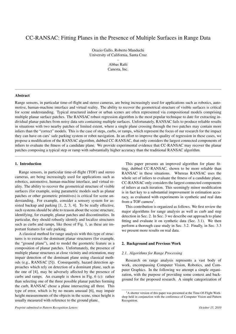
Figure 1: An example of a curb (a) and of a ramp (b). These types of featuresmust be identified for safe parking.

range analysis algorithms may be drawn based on whether lo-cal or global descriptors are employed. Local descriptors in-clude local surface normals [7, 8], ridges [9], and discontinu-ities [10, 11, 12, 13]. Contiguous point sets with similar localdescriptors may be clustered in space in order to identify ex-tended regions. For example, chains of points with high curva-ture may form a curb line, and groups of adjacent points withthe same normal may identify a planar patch. Only local anal-ysis of the range data is required for this type of descriptors,which can therefore be computed very quickly. For the samereason, however, local descriptors are susceptible to measure-ment noise and missing measurements.

“Global” descriptors, on the converse, are parametric rep-resentations (typically planar or quadratic) of relatively largesurface patches. All measurements in a patch contribute to theestimation of the parameters of the global descriptor. For ex-ample, if a set of measurements are known to be part of a plane,then simple linear regression (perhaps using principal compo-nent analysis, PCA) can provide the corresponding planar equa-tion.

When the measurements are affected by “outliers” (datapoints that differ substantially from the standard noise model),robust procedures should be employed [14, 15]. For example,M-estimators find the model parameters that minimize a cumu-lative “robust” loss function. With respect to the quadratic lossfunction used for standard linear regression, robust loss func-tions penalize more those samples that deviate heavily fromthe model. Possibly, the best known robust parametric esti-mators in Computer Vision are RANSAC [5] and the Houghtransform [16]. Both can be seen as particular instances of M-estimators [14]. Another popular robust estimation method isthe Least Median of Squares (LMedS) [17] and its variants,which include the Least K–th of Squares (LKS). It can be shownthat LMedS and LKS are instances of so-called S–estimators,which are a particular case of M–estimators [18]. Another ap-proach to dealing with outliers is to explicitly model them asuniformly distributed. This assumption is at the basis of theMLESAC algorithm [19].

An important parameter of robust estimators is the “scale”,ε, at which they operate. Intuitively, those points that are ata distance larger than ε from the estimated plane are consid-ered “outliers”; the remaining points are “inliers”. Clearly, thescale depends on the variance of the inliers, usually modeled

as normally distributed. The choice of scale may critically af-fect the performance of an estimator. A number of solutions tothe scale estimation problem exists, including joint estimationwith the model parameters [20], minimum unbiased scale esti-mation (MUSE [21]), adaptive least K–th order square estima-tion (ALKS [22]) and modified selective statistical estimation(MSSE [23]). When the variance of the inliers is not constant(heteroscedastic data), then more complex robust algorithmsshould be used [24].

In general, a given planar patch occupies only a finite por-tion in the image, with other, competing planar regions presentas well. There are three main approaches for the simultaneoussegmentation and estimation of planar regions in the same im-age. The first approach, which we use for the experiments inthis paper, is to simply use a robust estimator to extract a “dom-inant” planar region, by considering all the remaining points(including any other planar regions) as outliers. After findingthe planar region and removing the inliers, the operation is re-peated on the remaining points, until no more sizable planarstructures can be found. This algorithm is simple and intuitive,however, the presence of multiple structures may impair the es-timation of individual planar patches, especially if the scale isnot estimated correctly. This phenomenon was studied in de-tail [6, 18].

The second approach to multiple model estimation is to runa simultaneous, concurrent optimization over all planes visi-ble in the image. This can be obtained using the Expectation-Maximization algorithm (an iterative technique akin to K-means clustering) [25, 26] or the recently developed Gener-alized PCA algorithm [27]. In this case, each plane is repre-sented explicitly, rather than resorting to the notion of “outlier”with respect to a dominant structure. While intuitively more ap-pealing, this approach requires the joint estimation of the (un-known) number of planar surface elements in the scene, an op-eration that often proves challenging [28].

The third family of algorithms is based on region grow-ing [29, 30]. Starting from some “seed” points or regions, ho-mogeneous patches are grown concurrently by adding neigh-boring points consistent with the model. Regions that have sim-ilar models can then be merged together. Both region growingand merging can be performed using robust criteria [31, 32].Region growing is a simple and fast algorithm, but relies onthe selection of good seed points, which may be difficult to ob-tain, especially when planar patches of interest occupy only asmall portion of the image. Note that region growing can alsobe used as an initial step for subsequent robust parameter esti-mation [33].

2.2. Curb and Step Detection using Range DataCurb detection over short distances for safe driving has been

demonstrated at CMU with a laser striper [34]. The problemwith a fixed laser striper is that the viewing geometry is verylimited, while our task requires the ability to detect featuresover a rather wide field of view.

Se and Brady [35] used a stereo camera pair to detect curbsand steps. They detect candidate curbs by finding clusters oflines in an image using the Hough Transform. Then, in order

2

to classify a curb line as a step–up or step–down, they computethe ground plane parameters of the two regions separated by thecurb line. This allows one to precisely estimate the height of thecurb.

The work of Turchetto and Manduchi [36] combined stereoand visual information to find step edges. The idea behind thisapproach is that a curb’s edge usually generates a brightnessedge in the image, and thus, in the neighborhood of the pro-jected curb’s edge, the elevation gradient and the brightness gra-dient are expected to both have high values and to be aligned.Accordingly, detection is based on a weighted Hough Trans-form on brightness edge points, with weights values propor-tional to the scalar product of the brightness gradient and of thedepth gradient in the image.

This idea is pushed further in the work of Lu and Man-duchi [37]. For each surface element within a certain distancefrom an estimated ground plane, a surface curvature measure iscomputed on the range data, characterizing the likelihood thatthe point belongs to a curb or step edge. Segments in the imagethat are characterized by high brightness gradient (edges) andhigh surface curvature are extracted by means of a weightedHough transform. Finally, these segments are reprojected backinto the 3-D scene. The algorithm produced the endpoint of a3-D segment representing the curb edge, and could be used alsoto characterize staircases.

More recently, Pradeep et al. [38] proposed another stereo-based system for curb detection that is based on plane fitting.Tensor voting is used to calculate consistent normals at eachdata point, which allow for clustering into planar patches.

3. Regression and CC-RANSAC

As discussed previously, in the presence of curbs or smallsteps, dominant plane detection may produce unsatisfactory re-sults. This was noted, for example, by Lu and Manduchi [37],where it was shown that the estimated “ground plane” was notreliable enough for detection of small steps. In order to under-stand this behavior, it may be useful to quickly review somebasic concept of planar estimation.

Planar regression from a set of 3D point seeks for a plane Pthat minimizes some measure of observed “fitness” to the datapoints. If di is the Euclidian distance of the i-th data point to acandidate plane P, different measures of the fitness o(P) can beconsidered:

o = −∑

i d2i (LS)

o = −median{d2i } (LMedS)

o = |Iε(P)| (RANSAC)(1)

where Iε(P) is the set of inliers (i.e. data points with di ≤ εfor a given threshold ε) and |I| represents the cardinality of theset I. In the Least Squares approach (LS), the plane P withmaximum fitness o can be found in closed form. In the othertwo cases, random sampling can be used for minimization. Ingeneral, when the variance of the noise is known, at least ap-proximately, RANSAC is preferable to LMedS due to its lowercomputational cost. Both LMedS and RANSAC are superior to

LS when outliers are expected or, as in the scenarios consideredhere, when multiple planar models are present in the scene.

However, as mentioned earlier, even RANSAC (or LMedS)may provide poor results when the scene contains two or moreplanar patches at short distance from each other. This phe-nomenon was studied at length by Stewart [6]. This is not adefect of sampling: rather, the proposed measure of fitness ois not adequate, in the sense that the planes representing differ-ent surfaces in the scene do no necessarily produce large val-ues of fitness o. This is shown by way of example in Fig. 6.In this case, the plane that maximizes RANSAC fitness o (i.e.,the plane receiving the highest number of supporting inliers) isshown in a Fig. 6 (c). This plane straddles across the two planesrepresenting the top and bottom surfaces of a curb. Similar re-sults are obtained using the LMedS criterion.

Thus, even the robust fitness measures in 1 fail to correctlyidentify the individual visible planar components. We arguethat the main problem with such measures is that they neglectthe spatial coherence typically exhibited by inlier points. Ac-cordingly, we propose a modification of the RANSAC algo-rithm, dubbed CC-RANSAC, by defining the following mea-sure of fitness:

o = |IC(P)| (CC-RANSAC) (2)

where IC(P) is the largest connected component of inliers with8-neighbor topology inherited from the image grid. This ideaembeds the observation that data points that are the inliers of a“correct” plane cluster contiguously in space, whereas a planestraddling across two planar patches typically produces two dis-connected sets of inliers (see Fig. 6 (c)). Using IC for evaluatingthe fitness of a candidate plane ensures that only the inliers froma single planar patch will contribute to this measure. This is in-deed the case for Fig. 6 (d), where the red points represents theinliers belonging to IC for the same plane as in Fig. 6 (c).

3.1. Comparative Performance Assessment - Synthetic Data

In order to compare the performance of RANSAC and CC-RANSAC quantitatively, we first consider a synthetic data setwith noisy 3-D points generated from a model of a step. This al-lows us to test the algorithm under a wide variety of controlledconditions. A range imaging system is assumed to collect datafrom two planar patches (each providing 150 by 50 measure-ments on a regular grid with point spacing of 1 unit along eachaxis). The two patches, which are separated by a distance ofh units, are seen from above under orthography. The measure-ments are corrupted by Gaussian noise with standard deviationof σ units.

Our initial experiments computed robust planar regressionwith different values of the distance between the planar patches,h. Only one plane is estimated at each time. Since the twopatches have the same number of measurements, ideal robustregression would produce a plane modeling either patch. In or-der to measure the discrepancy between the plane P computedby the algorithm and the fitted patch, we compute the averagesquare distances {d

21, d

22} of the points of the two patches to

the plane P. Then, we define the regression error as e(P) =

3

Figure 2: Synthetically generated data representing a curb with height h equalto 5 units, with added Gaussian noise (in the vertical direction) with standarddeviation σ equal to 1 unit.

min(d1, d2). In each experiment, we first fix the number Nof random samples used for RANSAC or CC-RANSAC. Moreprecisely, a set of N non-collinear triplets of measurements aresampled without replacement from the data pool; the fitnessof the plane P identified by each triplet is computed using theRANSAC and the CC-RANSAC criteria; the best fitting planeis chosen for both cases, and a final least squares regressionbased on all the inliers is computed. This procedure is repeatedfor 500 times, each time with a new set of N triplets. The me-dian value e of regression error over the 500 experiments is usedfor the plots in the following figures.

2 4 6 8 100

0.5

1

1.5

h

e

ε=1N=500

Figure 3: Median regression error e as a function of the step height h usingRANSAC (stars) and CC-RANSAC (circles).

Fig. 3 shows the median regression error e when the distanceh between the two planar patches is varied. The value ε of thethreshold for the inliers (as defined in Sec. 2.1) is set equal to 1(i.e., equal to the standard deviation of noise). N=500 randomsamples are used for both algorithms. The most noteworthycharacteristic of the measurements in Fig. 3 is that, for h rang-ing between 4 and 8, RANSAC produces a relative large error,which drops to a low value for h > H, where H is a break-down value that in this case is approximately equal to 8. Thereason for this behavior is that for small values of h, RANSACproduces planes that straddle between the two patches. Whenthe patches are far enough from each other (relative to the mea-surement noise), RANSAC can produce stable and robust re-sults, reliably fitting either patch. The benefit of CC-RANSACis that the break-down value H is reduced from 8 to 3. In otherwords, CC-RANSAC allows for planar fitting in a wider rangeof step heights than RANSAC for the step considered in theseexperiments.

Next, we look at the performance of both algorithms when

0 0.5 1 1.5 2 2.5 30

0.5

1

1.5

2

2.5

3

ε

e

h=5N = 500

1 2 3 40

0.5

1

1.5

2

2.5

3

ε

e

h=10N=500

(a) (b)

Figure 4: Median regression error e as a function of inlier threshold ε usingRANSAC (stars) and CC-RANSAC (circles) for two different values of stepheight (h=5 and h=10).

the inliers threshold ε is changed. As mentioned earlier, a mea-surement point is considered an inlier with respect to a candi-date planePwhen its distance to P is less than ε. Robustness toincorrect (or “mismatched”) values of ε is important, since theactual standard deviation of noise σ is not always known withprecision. Fig. 4 (a) shows the median regression error e for astep of height h = 5 as ε is changed between 0.25 and 3 (whilethe standard deviation of noise σ remains equal to 1). It is seenthat RANSAC yields basically the same (large) regression er-ror, regardless of ε. CC-RANSAC produces reliable results forε between 0.5 and 1.25. For larger values of ε, it matches theresults of RANSAC. This is not surprising: for large enoughvalues of ε, an incorrect plane straddling across the two patcheswill produce a large number of connected inliers. The only timeCC-RANSAC performs worse than RANSAC is for very smallvalues of ε. The reason in this case is that only very small con-nected component are formed, which cannot provide reliablesupport for the correct plane.

Fig. 4 (b) shows results from a similar experiment, but thistime for a step with height h equal to 10 units. As seen in Fig. 3,at this step height RANSAC gives good results when ε is set to1. When ε takes values larger than 1.5, though, RANSAC pro-duces incorrect fitting planes with large median error. Remark-ably, the break-down point for CC-RANSAC is quite larger:only for ε larger than 3.5 does CC-RANSAC start behaving likeRANSAC.

0 100 200 300 400 5000

0.5

1

1.5

2

2.5

3

N

e

h=5ε=1

0 100 200 300 400 5000

0.5

1

1.5

2

2.5

3

N

e

h=10ε=1

(a) (b)

Figure 5: Median regression error e as a function of the number of randomsamples N using RANSAC (stars) and CC-RANSAC (circles) for two differentvalues of step height (h=5 and h=10). The bars show the 10- and 90-percentilesof the error distributions.

Finally, in Fig. 5 we show the median, along with the 10- and90-percentile, of the regression error as a function of the num-ber N of random samples used by the algorithms. When stepheight is set to 5 (with σ = ε = 1), CC-RANSAC produces

4

relatively stable results for N ≥ 100. Note that the medianerror for RANSAC remains basically constant, giving exper-imental evidence to the fact that incorrect regression is not aconsequence of poor sampling in this case. For h=10, the twoalgorithms perform substantially as well when N is changed.

3.2. Comparative Performance Assessment - TOF Measure-ments

Here we consider the measurements shown in Fig. 6 (a), ac-quired by a Canesta TOF camera in front of a curb, as a studycase. The goal is to find the prominent planar patch, shown inred in Fig. 6 (a). (Although there are two more planar patchesvisible in the scene, the one shown in red in Fig. 6 (b) has thelargest number of data points.)

Even when the ground truth planeP0 is available, it is impos-sible (or at least unpractical) to label each data point as belong-ing to a particular planar patch. This means that the regressionerror measure proposed in the previous section cannot be usedhere. We thus define a different “goodness” measure, that doesnot require knowledge of which patch each points belongs to.Given a candidate plane P, we define its quality q(P) as thenumber of inliers of P that are also inliers of the “ground truth”plane P0, normalized by the number of inliers of P0 :

q(P) = |I(P) ∩ I(P0)|/|I(P0)| (3)

Note that q(P) = 0 when P is far enough from the planar patch,and q(P) =1 when P coincides with P0. Hence, q seems like anappropriate and simple to compute measure for describing howwell a given plane fits the planar patch.2

Our first step is to compute the statistical correlation betweenfitness o of a candidate plane and its quality q. More precisely,we estimate the joint probability density function (pdf) of q ando, fq,o(q, o) by sampling the space of possible planes, where foreach plane sample P, o is set equal to either |Iε(P)| or to |IC(P)|based on the data of Fig. 6 (a). Note that, although the space ofcandidate planes is discrete (since each plane is determined bya triplet of measured points), we make the simplifying assump-tion that it is continuous in our analysis. The two joint pdf’s,computed using the Parzen window method from a set of 5000random sample planes, are shown in Fig. 7; these plots revealthat, for both choices of fitness, the joint pdf of q and o is char-acterized by two main “ridges”, corresponding to two differentclusters of planes.

We now show how fq,o(q, o) can be used to evaluate the ex-pected performance of RANSAC or CC-RANSAC. More pre-cisely, let qN be the random variable describing the quality ofthe plane chosen by either algorithm after N iterations (whereeach iteration corresponds to a randomly selected candidateplane). If {on} are the measured fitness values of the N can-didates planes, then each algorithm chooses the plane P witho(P) = o, where o = max{oi}.

The pdf of qN can be found as follows:

fqN (q) =

∫ ∞−∞

fqN |o(q|o) fo(o) do (4)

2Note that, as opposed to the regression error e used in the previous section,a high value of the quality q indicates good algorithm performance.

(a)

(b)

(c)

(d)

Figure 6: (a): Range data collected in front of a curb. (b): Optimal planar fit tothe lower planar patch (inliers with respect to the plane are shown in red). (c)Incorrect planar fit (P) and inliers in Iε(P). (d) Same plane as in (c) but withinliers in IC(P).

5

q

o

0 0.25 0.5 0.75 1

700

1400

2100

2800

q o

0 0.25 0.5 0.75 1

700

1400

2100

2800

(a) (b)

Figure 7: Graphical representation of the joint densities fq,o(q, o) for the dataof Fig. 6 (a) with (a) o = |Iε(P)| and (b) o = |ICC(P)|.

0.4 0.6 0.8 10

0.005

0.01

0.015

0.02

0.025

0.03

q

f q N(q)

N = 50N = 100N = 500N = 1000

0.4 0.6 0.8 10

0.005

0.01

0.015

0.02

0.025

0.03

q

f q N(q)

N = 50N = 100N = 500N = 1000

(a) (b)

Figure 8: Plots of the pdf fqN (q) of the quality of the plane chosen in the caseof Fig. 6 using (a) RANSAC and (b) CC-RANSAC with a variable number Nof iterations.

given that qN represents the quality of the plane with the highestfitness measure, it is clear that fqN |o(q|o) = fq|o(q|o). The pdf ofo can be easily derived based on the fact that the samples aredrawn independently:

fo(o) = N fo(o)FN−1o (o) (5)

where Fo(o) is the cumulative distribution function (cdf) of o:

Fo(o) =

∫ o

−∞

fo(u) du (6)

All of those quantities are easily computed by numerical inte-gration starting from fq,o(q, o).

Fig. 8 shows the pdf fqN (q) for RANSAC and CC-RANSACfor different numbers N of iterations. It is interesting to notethat RANSAC yields a bimodal distribution: since the twoplanes of Fig. 6 (a) and (c) both receive good inlier support, thealgorithm may choose one or the other with almost the samelikelihood (although the incorrect plane receives higher proba-bility mass as the number of iterations increases). RANSAC-CC, instead, yields a unimodal distribution that is peakedaround a high quality value, meaning that it almost invariablychooses a plane that is close to the optimal one. Even if only alimited amount of iterations (e.g., 100) is used, the chosen planeis likely to have a good quality value.

3.3. Planar Fitting Examples for Curbs and RampsThis section presents a few experimental results using CC-

RANSAC, in order to highlight the potential of this approachfor curb and ramp detection. These examples are of interest forautomotive applications, such as safe parking systems. Notethat, although we only present results for ramps and steps, these

patterns can be regarded as the building blocks for virtuallyany structure that only comprises planar surfaces. For exam-ple, an indoor staircase, which could be useful to detect for au-tonomous or semi-autonomous navigation (e.g., for the assistedcontrol of a motor wheelchair [39]), can be seen as a sequenceof steps. The crucial aspect, regardless of the structure, is thatenough datapoints support each planar patch; in the case of au-tonomous navigation, for example, a staircase would probablybe seen as a ramp from a distance and the steps would becomevisible as the robot or the wheelchair approaches it.

In Fig. 9, as well as in Fig. 6, inliers are represented withthick points, with color indicating to the plane they are closestto. For each fitting plane, we show the convex hull of its closestinliers, projected onto the planes.

Fig. 9 (a) shows the three best fitting planes to the data ofFig. 6. After the dominant plane has been found, the corre-sponding inliers are removed from the data, and the operationis repeated until a maximum number of planes is found, or thehighest planar fitness for the remaining point is below a certainthreshold.

Fig. 9 (b) shows the result to a similar curb taken from alarger distance. In this case, only two fitting planes were found.Note that the fit is pretty good, in spite of the planar patchesbeing close to each other.

Examples of ramp modeling are shown in Fig. 9 (c) and (d).In particular, Fig. 9 (d) is based on measurements taken of theramp shown in Fig. 1 (b). The red planar patch correspondsto the descending concrete surface in the ramp; the blue patchrepresents the asphalt surface at the bottom of the ramp; whilethe green patch corresponds to the surface covered in soil to theleft of the ramp. Note that, contrary to what one would hope,the green and the blue patches do not intersect. This is due tothe fact that the measurements supporting the green patch arebiased by the presence of a tree stump, visible near the left edgeof Fig. 1. Nonetheless, the algorithm is shown to produce verygood planar fits to the different elements of the scene, whichmay enable further reasoning and recognition.

4. Conclusions

The ability to accurately measure the geometry of the sceneenables systems relying on range sensors, for instance TOF sen-sors, to recognize features that are critical for many applica-tions, such as safe parking. In this paper we concentrate onsituations where this task can be impaired by the presence ofmultiple planar structures as in the case of curbs and ramps,a situation that is extremely common in urban environments.These are particularly challenging features that cannot be re-liably detected using conventional ultrasound and microwavesensors.

In order to describe the geometry of a curb or of a ramp,we perform robust fitting to the different visible planar patches.We have shown that the popular RANSAC algorithm may failin the case of a shallow curb; this result is in agreement withprevious work by Stewart [6]. In order to deal with these sit-uations, we propose a new algorithm, CC-RANSAC, that uses

6

only the largest connected component of inliers to evaluate thefitness of a candidate plane. This seemingly minor modificationmay in fact yield substantially better fits than RANSAC.

A critical analysis of CC-RANSAC brings a consideration tolight. The assumption that inliers cluster together into one largeconnected component, although intuitively correct, needs to beinvestigated further. It is clear that the size of the largest con-nected component depends on the distribution of the distancesdi of the data points to the candidate plane as well as on thechosen threshold ε. If ε is too small, only isolated inlier clus-ters will form, as shown by our experiments of Sec. 3.1. If εis too large, clusters of inliers corresponding to different planarpatches may end up connecting with each other.

In future work we will investigate methods to increase therobustness of this approach by considering different ways tocluster the inliers. For example, one could use the isophoticmetric [40], that combines Eulidean distance and distance be-tween normals. This could help in situations with “holes” in therange data, which are liable to create multiple connected com-ponents where only one connected component is expected3.

References

[1] V. Glazduri, An investigation of the potential safety benefits of vehiclebackup proximity sensors, in: Proceedings of the International TechnicalConference on Enhanced Safety Vehicles, 2005.

[2] M. Paine, M. Henderson, Devices to assist in reducing the risk to youngpedestrians from reversing motor vehicles, technical Specification 149,Roads and Traffic Authority, New South Wales, Australia (October 2005).

[3] Backup systems, Consumer Reports 69 (10) (2004) 19–20.[4] S. Hsu, A. Rafii, D. Hirvonen, Object detection and tracking using an

optical time-of-flight range camera module for vehicle safety and driverassist applications, in: Proceedings of SAE World Congress & Exhibition,2007.

[5] M. A. Fischler, R. C. Bolles, Random sample consensus: aparadigm for model fitting with applications to image analysis andautomated cartography, Commun. ACM 24 (6) (1981) 381–395.doi:http://doi.acm.org/10.1145/358669.358692.

[6] C. V. Stewart, Bias in robust estimation caused by discontinuities andmultiple structures, IEEE Transactions on Pattern Analysis and MachineIntelligence 19 (8) (1997) 818–833.

[7] J. F. Lalonde, R. Unnikrishnan, N. Vandapel, M. Hebert, Scale selectionfor classification of point-sampled 3D surfaces, in: Fifth InternationalConference on 3-D Digital Imaging and Modeling (3DIM 2005), 2005,pp. 285–292.

[8] N. J. Mitra, A. Nguyen, L. Guibas, Estimating surface normals in noisypoint cloud data, International Journal of Computational Geometry andApplications 14 (4–5) (2004) 261–276.

[9] D. Eberly, R. Gardner, B. Morse, S. Pizer, C. Scharlach, Ridges for imageanalysis, Journal of Mathematical Imaging and Vision 4 (4) (1994) 353–373. doi:http://dx.doi.org/10.1007/BF01262402.

[10] F. Tang, M. Adams, J. Ibanez-Guzman, W. S. Wijesoma, Pose invariant,robust feature extraction from data with a modified scale space approach,Proceedings of the IEEE International Conference on Robotics and Au-tomation (ICRA ’04) 3 (2004) 3173–3179.

[11] W.-S. Tong, C.-K. Tang, G. Medioni, First order tensor voting, and appli-cation to 3-D scale analysis, in: Proceedings of the IEEE Conference onComputer Vision and Pattern Recognition (CVPR ’01), Vol. 1, 2001.

[12] M. Adams, A. Kerstens, Tracking naturally-occurring indoor featuresin 2-D and 3-D with lidar range amplitude data, Internation Journal ofRobotics Research 17 (9) (1998) 907–923.

3We thank the anonymous reviewer for this suggestion.

(a)

(b)

(c)

(d)

Figure 9: Some experimental results with curbs ((a) and (b)) and ramps ((c) and(d)).

7

[13] M. D. Adams, On-line gradient based surface discontinuity detection foroutdoor scanning range sensors, in: Proceedings of the IEEE/RSJ Interna-tional Conference on Intelligent Robots and Systems (IROS ’01), Vol. 3,2001, pp. 1726–1731.

[14] C. V. Stewart, Robust parameter estimation in computer vision, SIAMRev. 41 (3) (1999) 513–537.

[15] P. Meer, Robust techniques for computer vision, in: G. Medioni, S. B.Kang (Eds.), Emerging Topics in Computer Vision, 1st Edition, IMSCPress Multimedia Series, Prentice Hall, 2004, Ch. 4.

[16] J. Illingworth, J. Kittler, A survey of the Hough transform,Comput. Vision Graph. Image Process. 44 (1) (1988) 87–116.doi:http://dx.doi.org/10.1016/S0734-189X(88)80033-1.

[17] P. Rousseeuw, A. Leroy, Robust regression and outlier detection, JohnWiley & Sons, Inc., New York, NY, USA, 1987.

[18] H. Chen, P. Meer, D. E. Tyler, Robust regression for data with multiplestructures, in: Proceedings of the IEEE Conference on Computer Visionand Pattern Recognition (CVPR 2001), Vol. 1, 2001, pp. 1069–1075.

[19] P. H. S. Torr, A. Zisserman, MLESAC: a new robust esti-mator with application to estimating image geometry, Com-puter Vision and Image Understanding 78 (1) (2000) 138–156.doi:http://dx.doi.org/10.1006/cviu.1999.0832.

[20] P. Huber, Robust Statistics, Wiley, New York, 1981.[21] J. V. Miller, C. V. Stewart, MUSE: robust surface fitting using unbiased

scale estimates, in: Proceedings of the IEEE Conference onComputer Vi-sion and Pattern Recognition (CVPR ’96), 1996, pp. 300–306.

[22] K.-M. Lee, P. Meer, R.-H. Park, Robust adaptive segmentation of rangeimages, IEEE Transactions on Pattern Analysis and Machine Intelligence20 (2) (1998) 200–205.

[23] A. Bab-Hadiashar, D. Suter, Robust range segmentation, in: Proceedingsof the Fourteenth International Conference on Pattern Recognition, Vol. 2,1998, pp. 969–971.

[24] R. Subbarao, P. Meer, Heteroscedastic projection based m-estimators, in:Proceedings of the IEEE Conference on Computer Vision and PatternRecognition (CVPR ’05), Vol. 3, 2005, pp. 38–38.

[25] Y. Liu, R. Emery, D. Chakrabarti, W. Burgard, S. Thrun, Using EM tolearn 3D models with mobile robots, in: Proceedings of the InternationalConference on Machine Learning (ICML), 2001.

[26] R. Triebel, W. Burgard, F. Dellaert, Using hierarchical EM to extractplanes from 3D range scans, Proceedings of the 2005 IEEE InternationalConference on Robotics and Automation (ICRA 2005) (2005) 4437–4442.

[27] R. Vidal, Y. Ma, S. Sastry, Generalized principal compo-nent analysis (GPCA), IEEE Transactions on Pattern Anal-ysis and Machine Intelligence 27 (12) (2005) 1945–1959.doi:http://doi.ieeecomputersociety.org/10.1109/TPAMI.2005.244.

[28] G. McLachlan, D. Peel, Finite Mixture Models, Wiley-Interscience, 2000.[29] P. J. Besl, R. C. Jain, Segmentation through variable-order surface fitting,

IEEE Transactions on Pattern Analysis and Machine Intelligence 10 (2)(1988) 167–192.

[30] G. Taubin, Estimation of planar curves, surfaces, and nonplanar spacecurves defined by implicit equations with applications to edge and rangeimage segmentation, IEEE Transactions on Pattern Analysis and MachineIntelligence 13 (11) (1991) 1115–1138.

[31] K. Boyer, M. Mirza, G. Ganguly, The robust sequential esti-mator: A general approach and its application to surface or-ganization in range data, IEEE Transactions on Pattern Anal-ysis and Machine Intelligence 16 (10) (1994) 987–1001.doi:http://doi.ieeecomputersociety.org/10.1109/34.329010.

[32] K. Koster, M. Spann, MIR: an approach to robust clustering-applicationto range image segmentation, IEEE Transactions on Pattern Analysis andMachine Intelligence 22 (5) (2000) 430–444.

[33] R. Unnikrishnan, M. Hebert, Robust extraction of multiple structuresfrom non-uniformly sampled data, Proceedings of the IEEE/RSJ Inter-national Conference on Intelligent Robots and Systems (IROS 2003) 2(2003) 1322–1329 vol.2.

[34] R. Aufrere, C. Mertz, C. Thorpe, Multiple sensor fusion for detectinglocation of curbs, walls, and barriers, in: Proceedings of the IEEE Intelli-gent Vehicles Symposium, 2003, pp. 126–131.

[35] S. Se, J. Brady, Vision-based detection of kerbs and steps, in: Proceedingsof the British Machine Vision Conference (BMVC ’97), 1997, pp. 410–419.

[36] R. Turchetto, R. Manduchi, Visual curb localization for autonomous nav-igation, in: Proceedings of the IEEE/RSJ International Conference on In-telligent Robots and Systems (IROS 2003), Vol. 2, 2003, pp. 1336–1342.

[37] X. Lu, R. Manduchi, Detection and localization of curbs and stairwaysusing stereo vision, in: Proceedings of the IEEE International Conferenceon Robotics and Automation (ICRA 2005), 2005, pp. 4648–4654.

[38] V. Pradeep, G. Medioni, J. Weiland, Piecewise planar modeling for stepdetection using stereo vision, in: Computer Vision Applications for theVisually Impaired (CVAVI’08), Marseille, France, 2008.

[39] M. J. Murarka, A., B. Kuipers.[40] H. Pottmann, T. Steiner, M. Hofer, C. Haider, A. Hanbury, The isophotic

metric and its application to feature sensitive morphology on surfaces, in:Proc. ECCV 2004, 2004, pp. 560–572.

8