causality and graphical models in time series analysisgalton.uchicago.edu/~eichler/hsss.pdf · 1...

1Causality and graphical models in time series

analysis

Rainer Dahlhaus and Michael EichlerUniversitat Heidelberg

1 IntroductionOver the last years there has been growing interest in graphical models and inparticular in those based on directed acyclic graphs as a general framework todescribe and infer causal relations (Pearl 1995, 2000; Lauritzen 2000; Dawid2000). This new graphical approach is related to other approaches to formalizethe concept of causality such as Neyman and Rubin’s potential-response model(Neyman 1935; Rubin 1974; Robins 1986) and path analysis or structural equa-tion models (Wright 1921; Haavelmo 1943). The latter concept has been appliedin particular by economists to describe the equilibrium distributions of systemswhich typically evolve over time.

In this chapter we take up the idea behind the dynamic interpretation ofstructural equations and discuss (among others) graphical models in which theflow of time is exploited for causal inference. Instead of the intervention basedcausality concept used by Pearl (1995) and others we apply a simpler notionof causality which is based on the obvious fact that an effect cannot precedeits cause in time. Assuming that the variables are observed at different timepoints the noncausality relations in the system can be derived by examining the(partial) correlation between the variables at different time lags. In the sameway we are able to identify the direction of directed edges in the graphical modelsthus avoiding the assumption of an a priori given ordering of the variables ase.g. in directed acyclic graphs for multivariate data. Since we have repeatedmeasurements of the variables over time we are in a time series setting. Morerestrictively we focus in this chapter on the situation where we observe only onelong multivariate, stationary time series (in contrast, for example, to the panelsituation where we have multiple observations of possibly short series).

The concept of causality we use is the concept of Granger causality (Granger1969) which exploits the natural time ordering to achieve a causal ordering ofthe variables. More precisely, one time series is said to be Granger causal foranother series if we are better able to predict the latter series using all availableinformation than if the information apart from the former series had been used.This concept of causality has been discussed extensively in the econometrics

2 R. Dahlhaus and M. Eichler

literature, with several extensions and modifications. Eichler (1999, 2000) hasused the definition of Granger causality to define causality graphs for time series.We discuss these graphs in Section 2 together with time series chain graphs andpartial correlation graphs for time series (Dahlhaus 2000). In Section 3 we discussMarkov properties and in Section 4 statistical inference for these graphs. Section5 contains two data examples. Finally Section 6 offers some concluding remarks.In particular we discuss the use of the presented graphs for causal inference andpossible sources for wrong identification of causal effects.

2 Graphical models for multivariate time series.Let X = {Xa(t), t ∈ Z, a = 1, . . . , d} be a d-variate stationary process. Through-out the chapter we assume that X has positive definite spectral matrix f(λ)with eigenvalues bounded and bounded away from zero uniformly for all λ ∈[−π, π]. Let V = {1, . . . , d} be the set of indices. For any A ⊆ V we defineXA = {XA(t)} as the multivariate subprocess given by the indices in A. FurtherXA(t) = {XA(s), s < t} denotes the past of the subprocess XA at time t.

There exist several possibilities for defining graphical models for a time seriesX. We can distinguish between two classes of graphical models. In the first classthe variable Xa(t) at a specific time t is represented by a separate vertex in thegraph. This leads to generalizations of classical graphical models such as the timeseries chain graph introduced in Definition 2.1. In the second class of graphicalmodels the vertex set only consists of the components Xa of the series, whichleads to a coarser modelling of the dependence structure of the series. As wewill see below this leads to mixed graphs in which directed edges reflect Grangercausality whereas the contemporaneous dependence structure is represented byundirected edges. These graphs are termed Granger causality graphs (Definition2.4). In addition we have also partial correlation graphs for time series (Definition2.6) which generalize classical concentration graphs to the time series situation.

Here we restrict ourselves to linear association and linear Granger noncausal-ity, which formally can be expressed in terms of conditional orthogonality ofclosed linear subspaces in a Hilbert space of random variables (e.g. Eichler 2000,Appendix A.1). For random vectors X, Y , and Z, X and Y are conditionallyorthogonal given Z, denoted by X ⊥ Y |Z, if X and Y are uncorrelated afterthe linear effects of Z have been removed. It is clear that this linear approachcannot capture the full causal relationships of processes which are partly of non-linear nature. The need for this restriction results from problems in statisticalinference. For example, there exist nonparametric methods for estimating lineardependencies whereas in the general case nonparametric inference seems hardlypossible particularly in view of the curse of dimensionality. Even if parametricmodels are used, inference for nonlinear models is often impractical due to alarge number of parameters and many applications therefore are restricted tolinear models. We note that the graphical modelling approach can be extendedto the nonlinear case by replacing conditional orthogonality by conditional in-dependence which leads to the notion of strong Granger causality (Eichler 2000,

Causality and graphical models in time series analysis 3

Sect. 5; Eichler 2001). For Gaussian processes the two meanings of the graphsof course are identical. Large parts of the results in this chapter also hold forthese general graphs. For details we refer to the discussion in Section 6.

2.1 Time series chain graphs

The first approach for defining graphical time series models naturally leads tochain graphs. Lynggaard and Walther (1993) introduced dynamic interactionmodels for time series based on the classical LWF Markov property for chaingraphs (cf. Lauritzen and Wermuth 1989; Frydenberg 1990). Here we discussan alternative approach which defines the graph according to the AMP Markovproperty of Andersson, Madigan, and Perlman (2001). One reason for this is thatthere exists an intimate relation between the use of the AMP Markov propertyin time series chain graphs and the recursive structure of a large number of timeseries models which then immediately characterize the graph. Another reasonis that the AMP Markov property is related to the notion of Granger causalitywhich is used in the definition of Granger causality graphs. In particular theAMP Markov property allows to obtain the Granger causality graph from thetime series chain graph by simple aggregation.

Definition 2.1 (Time series chain graph) The time series chain graph (TSC-graph) of a stationary process X is the chain graph GTS = (VTS, ETS) withVTS = V × Z and edge set ETS such that

(a, t− u)−→ (b, t) /∈ ETS ⇔ u ≤ 0 or Xa(t− u) ⊥ Xb(t) |XV (t)\{Xa(t− u)},(a, t− u)−− (b, t) /∈ ETS ⇔ u 6= 0 or Xa(t) ⊥ Xb(t) |XV (t) ∪ {XV \{a,b}(t)}.

Since the process is stationary we have (a, t)−−(b, t) /∈ ETS if and only if (a, s)−−(b, s) /∈ ETS for all s ∈ Z. The same shift invariance also holds for the directededges. We further note that the above conditions guarantee that the processsatisfies the pairwise AMP Markov property for GTS (Andersson et al. 2000).

Example 2.2 (Vector autoregressive processes) Suppose X is a linear vectorautoregressive (VAR) process

X(t) = A(1)X(t− 1) + . . .+A(p)X(t− p) + ε(t) (2.1)

where the errors ε(t) are independent and identically distributed with mean 0and covariance matrix Σ. If GTS = (VTS, ETS) denotes the TSC-graph then itcan be shown that

(a, t− u)−→ (b, t) ∈ ETS ⇔ u ∈ {1, . . . , p} and Aba(u) 6= 0, (2.2)

i.e. the directed edges in the graph reflect the recursive structure of the timeseries. Furthermore the undirected edges specify a covariance selection model(e.g. Dempster 1972) for the errors ε(t) and we have with K = Σ−1

(a, t)−− (b, t) ∈ ETS ⇔ εa(t) ⊥ εb(t) | εV \{a,b}(t) ⇔ Kab 6= 0.


t-3 t-2 t-1 t

5

4

3

2

1

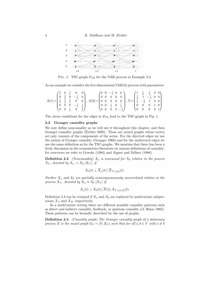
Fig. 1. TSC-graph GTS for the VAR process in Example 2.2.

As an example we consider the five-dimensional VAR(2)-process with parameters

A(1)=

35

0 15

0 0

0 35

0 − 15

025

13

35

0 0

0 0 0 − 12

15

0 0 15

0 25

, A(2)=

0 0 − 1

50 0

0 0 0 0 0

0 0 0 0 0

0 0 15

0 13

0 0 0 0 − 15

, Σ=

1 1

213

0 012

1 − 13

0 013− 1

31 0 0

0 0 0 1 0

0 0 0 0 1

.

The above conditions for the edges in ETS lead to the TSC-graph in Fig. 1.

2.2 Granger causality graphs

We now define noncausality as we will use it throughout this chapter, and thenGranger causality graphs (Eichler 2000). These are mixed graphs whose vertexset only consists of the components of the series. For the directed edges we usethe notion of Granger causality (Granger 1969) and for the undirected edges weuse the same definition as for the TSC-graphs. We mention that there has been alively discussion in the econometrics literature on various definitions of causality;for overviews we refer to Geweke (1984) and Aigner and Zellner (1988).

Definition 2.3 (Noncausality) Xa is noncausal for Xb relative to the processXV , denoted by Xa 9 Xb [XV ], if

Xb(t) ⊥ Xa(t) |XV \{a}(t).

Further Xa and Xb are partially contemporaneously uncorrelated relative to theprocess XV , denoted by Xa � Xb [XV ] if

Xa(t) ⊥ Xb(t) |X(t), XV \{a,b}(t).

Definition 2.3 can be retained if Xa and Xb are replaced by multivariate subpro-cesses XA and XB , respectively.

In a multivariate setting there are different possible causality patterns suchas direct and indirect causality, feedback, or spurious causality (cf. Hsiao 1982).These patterns can be formally described by the use of graphs.

Definition 2.4 (Causality graph) The Granger causality graph of a stationaryprocess X is the mixed graph GC = (V,EC) such that for all a, b ∈ V with a 6= b


1

2 4

53

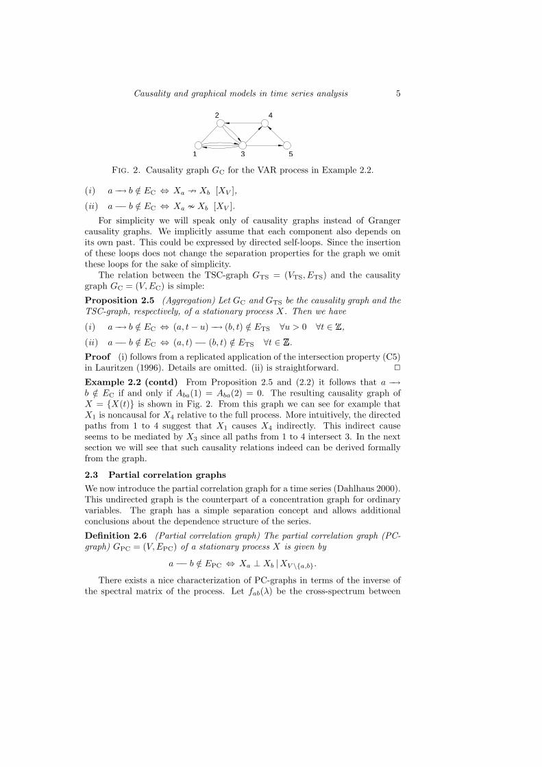
Fig. 2. Causality graph GC for the VAR process in Example 2.2.

(i) a−→ b /∈ EC ⇔ Xa 9 Xb [XV ],

(ii) a−− b /∈ EC ⇔ Xa � Xb [XV ].

For simplicity we will speak only of causality graphs instead of Grangercausality graphs. We implicitly assume that each component also depends onits own past. This could be expressed by directed self-loops. Since the insertionof these loops does not change the separation properties for the graph we omitthese loops for the sake of simplicity.

The relation between the TSC-graph GTS = (VTS, ETS) and the causalitygraph GC = (V,EC) is simple:

Proposition 2.5 (Aggregation) Let GC and GTS be the causality graph and theTSC-graph, respectively, of a stationary process X. Then we have

(i) a−→ b /∈ EC ⇔ (a, t− u)−→ (b, t) /∈ ETS ∀u > 0 ∀t ∈ Z,

(ii) a−− b /∈ EC ⇔ (a, t)−− (b, t) /∈ ETS ∀t ∈ Z.

Proof (i) follows from a replicated application of the intersection property (C5)in Lauritzen (1996). Details are omitted. (ii) is straightforward. 2

Example 2.2 (contd) From Proposition 2.5 and (2.2) it follows that a −→b /∈ EC if and only if Aba(1) = Aba(2) = 0. The resulting causality graph ofX = {X(t)} is shown in Fig. 2. From this graph we can see for example thatX1 is noncausal for X4 relative to the full process. More intuitively, the directedpaths from 1 to 4 suggest that X1 causes X4 indirectly. This indirect causeseems to be mediated by X3 since all paths from 1 to 4 intersect 3. In the nextsection we will see that such causality relations indeed can be derived formallyfrom the graph.

2.3 Partial correlation graphs

We now introduce the partial correlation graph for a time series (Dahlhaus 2000).This undirected graph is the counterpart of a concentration graph for ordinaryvariables. The graph has a simple separation concept and allows additionalconclusions about the dependence structure of the series.

Definition 2.6 (Partial correlation graph) The partial correlation graph (PC-graph) GPC = (V,EPC) of a stationary process X is given by

a−− b /∈ EPC ⇔ Xa ⊥ Xb |XV \{a,b}.

There exists a nice characterization of PC-graphs in terms of the inverse ofthe spectral matrix of the process. Let fab(λ) be the cross-spectrum between


1 3 5

42

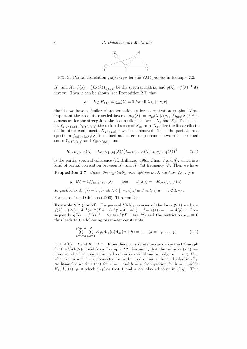
Fig. 3. Partial correlation graph GPC for the VAR process in Example 2.2.

Xa and Xb, f(λ) =(fab(λ)

)a,b∈V be the spectral matrix, and g(λ) = f(λ)−1 its

inverse. Then it can be shown (see Proposition 2.7) that

a−− b 6∈ EPC ⇔ gab(λ) = 0 for all λ ∈ [−π, π].

that is, we have a similar characterization as for concentration graphs. Moreimportant the absolute rescaled inverse |dab(λ)| = |gab(λ)|/

(gaa(λ)gbb(λ)

)1/2 is

a measure for the strength of the “connection” between Xa and Xb. To see thislet Ya|V \{a,b}, Yb|V \{a,b} the residual series of Xa, resp. Xb after the linear effectsof the other components XV \{a,b} have been removed. Then the partial crossspectrum fab|V \{a,b}(λ) is defined as the cross spectrum between the residualseries Ya|V \{a,b} and Yb|V \{a,b}, and

Rab|V \{a,b}(λ) = fab|V \{a,b}(λ)/(faa|V \{a,b}(λ)fbb|V \{a,b}(λ)

) 12 (2.3)

is the partial spectral coherence (cf. Brillinger, 1981, Chap. 7 and 8), which is akind of partial correlation between Xa and Xb “at frequency λ”. Then we have

Proposition 2.7 Under the regularity assumptions on X we have for a 6= b

gaa(λ) = 1/faa|V \{a}(λ) and dab(λ) = −Rab|V \{a,b}(λ).

In particular dab(λ) = 0 for all λ ∈ [−π, π] if and only if a−− b 6∈ EPC .

For a proof see Dahlhaus (2000), Theorem 2.4.

Example 2.2 (contd) For general VAR processes of the form (2.1) we havef(λ) = (2π)−1A−1(e−iλ)ΣA−1(eiλ)′ with A(z) = I −A(1)z− . . .−A(p)zp. Con-sequently g(λ) = f(λ)−1 = 2πA(eiλ)′Σ−1A(e−iλ) and the restriction gab ≡ 0thus leads to the following parameter constraints

p∧p+h∑u=0∨h

d∑j,k=1

KjkAja(u)Akb(u+ h) = 0, (h = −p, . . . , p) (2.4)

with A(0) = I and K = Σ−1. From these constraints we can derive the PC-graphfor the VAR(2)-model from Example 2.2. Assuming that the terms in (2.4) arenonzero whenever one summand is nonzero we obtain an edge a −− b ∈ EPC

whenever a and b are connected by a directed or an undirected edge in GC.Additionally we find that for a = 1 and b = 4 the equation for h = 1 yieldsK12A24(1) 6= 0 which implies that 1 and 4 are also adjacent in GPC. This


leads to the PC-graph in Figure 3. In general further conditional orthogonalitiesare possible under additional restrictions on the parameters. However, for thisparticular model an elaborate examination shows that this is not the case.

The condition K12A24(1) 6= 0 in the example implies that 1 −− 2←− 4 is asubgraph of GC. After insertion of the edge 1−− 4 this subgraph becomes com-plete, that is, any two vertices in the subgraph are adjacent. Thus the PC-graphof the process has been obtained from the causality graph by completing thissubgraph and then converting all directed edges to undirected edges. This oper-ation is called moralization. In the next section we will see that this relationshipbetween the causality graph and the PC-graph holds for all processes satisfyingthe regularity assumptions in Section 2.

Summarizing the three graphs GTS, GC, and GPC are related by two map-pings which correspond to the operations of aggregation and moralization,

GTS 7Prop. 2.5−−−−−−→ GC 7

Rem. 3.5−−−−−→ GPC.

Thus the graphs in a certain sense visualize the dependence structure of theprocess at different resolution levels, the TSC-graph having the finest resolution.

3 Markov propertiesThe time series graphs introduced in the previous section visualize the pairwiseinteraction structure between the components of the process, i.e. they reflect thepairwise Markov properties of the process. The interpretation of the graphs isenhanced by global Markov properties which relate the separation properties of agraph to conditional orthogonality or causality relations between the componentsof the process. For graphs which contain directed edges there are two mainapproaches defining global Markov properties: One approach utilizes separationin undirected graphs by applying the operation of moralization to appropriatesubgraphs while the other approach is based on path-oriented criteria like d-separation (Pearl, 1988) for directed acyclic graphs.

3.1 Global Markov properties for PC-graphs

Partial correlation graphs generalize concentration graphs for multivariate vari-ables. Thus the corresponding global Markov property is naturally based onthe separation in undirected graphs. For an undirected graph G = (V,E) anddisjoint subsets A,B, S ⊆ V we say that S separates A and B, denoted byA 1 B |S [G], if every path between A and B in G necessarily intersects S.Then the following result was shown by Dahlhaus (2000).

Theorem 3.1 Let GPC = (V,EPC) be the partial correlation graph of X. Thenfor all disjoint subsets A, B, S of V

A 1 B |S [GPC] ⇒ XA ⊥ XB |XS .

We say that X satisfies the global Markov property for GPC.


a

c

b a

dc

ba b

c

(b) (c)(a)

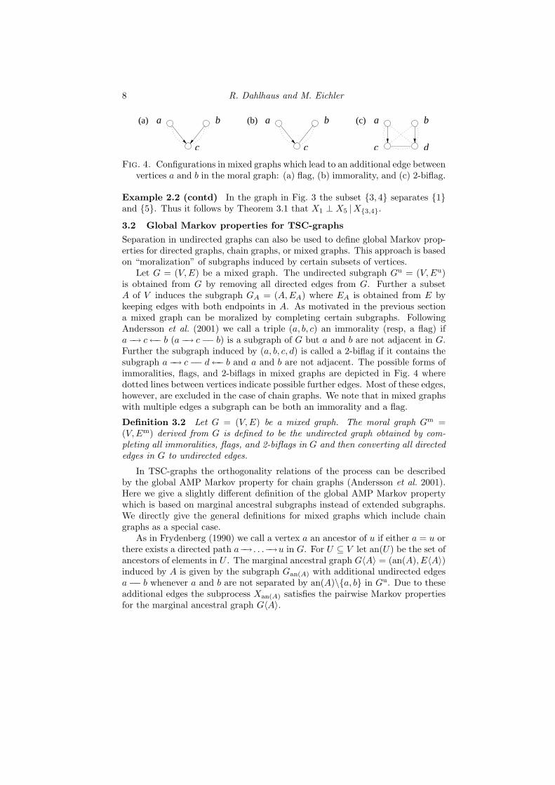
Fig. 4. Configurations in mixed graphs which lead to an additional edge betweenvertices a and b in the moral graph: (a) flag, (b) immorality, and (c) 2-biflag.

Example 2.2 (contd) In the graph in Fig. 3 the subset {3, 4} separates {1}and {5}. Thus it follows by Theorem 3.1 that X1 ⊥ X5 |X{3,4}.

3.2 Global Markov properties for TSC-graphs

Separation in undirected graphs can also be used to define global Markov prop-erties for directed graphs, chain graphs, or mixed graphs. This approach is basedon “moralization” of subgraphs induced by certain subsets of vertices.

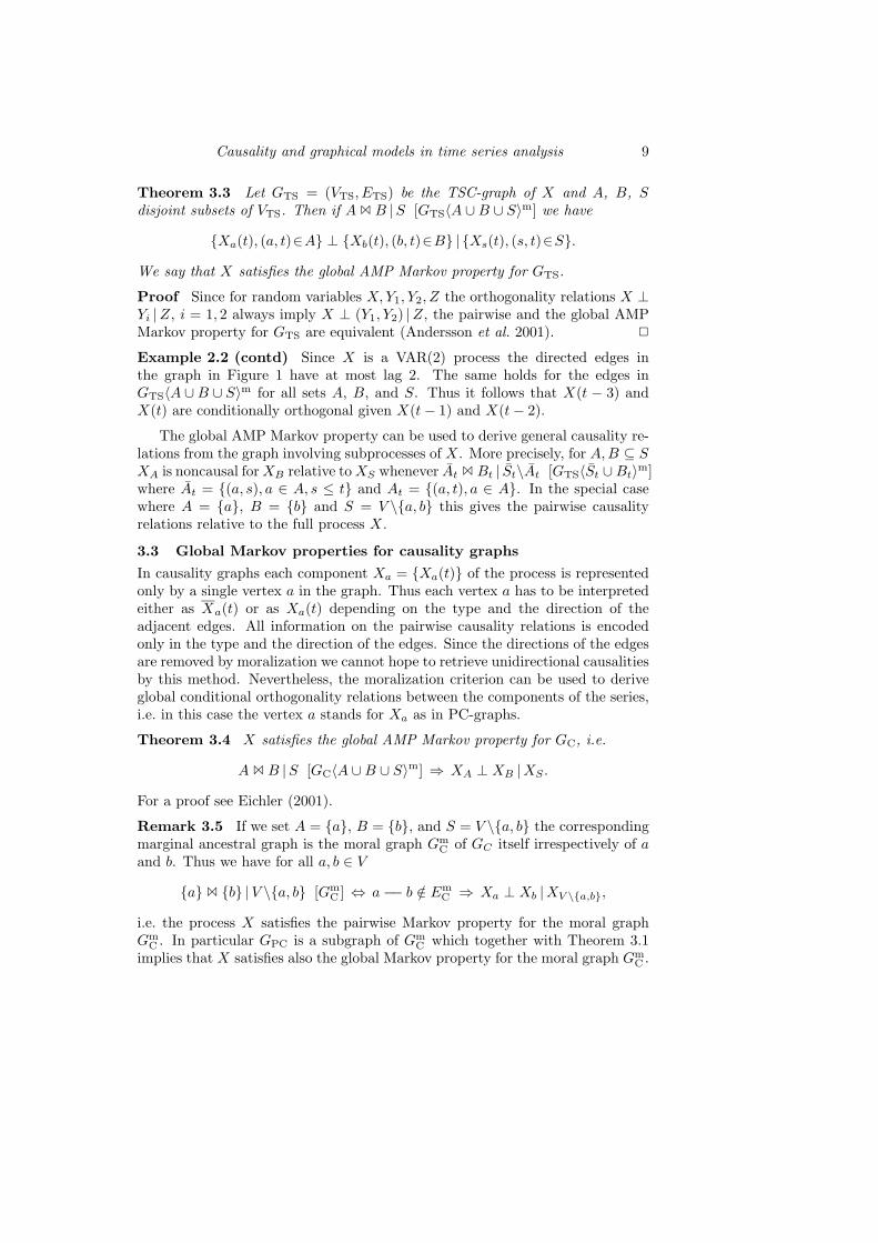
Let G = (V,E) be a mixed graph. The undirected subgraph Gu = (V,Eu)is obtained from G by removing all directed edges from G. Further a subsetA of V induces the subgraph GA = (A,EA) where EA is obtained from E bykeeping edges with both endpoints in A. As motivated in the previous sectiona mixed graph can be moralized by completing certain subgraphs. FollowingAndersson et al. (2001) we call a triple (a, b, c) an immorality (resp, a flag) ifa−→ c←− b (a−→ c−− b) is a subgraph of G but a and b are not adjacent in G.Further the subgraph induced by (a, b, c, d) is called a 2-biflag if it contains thesubgraph a−→ c−− d←− b and a and b are not adjacent. The possible forms ofimmoralities, flags, and 2-biflags in mixed graphs are depicted in Fig. 4 wheredotted lines between vertices indicate possible further edges. Most of these edges,however, are excluded in the case of chain graphs. We note that in mixed graphswith multiple edges a subgraph can be both an immorality and a flag.

Definition 3.2 Let G = (V,E) be a mixed graph. The moral graph Gm =(V,Em) derived from G is defined to be the undirected graph obtained by com-pleting all immoralities, flags, and 2-biflags in G and then converting all directededges in G to undirected edges.

In TSC-graphs the orthogonality relations of the process can be describedby the global AMP Markov property for chain graphs (Andersson et al. 2001).Here we give a slightly different definition of the global AMP Markov propertywhich is based on marginal ancestral subgraphs instead of extended subgraphs.We directly give the general definitions for mixed graphs which include chaingraphs as a special case.

As in Frydenberg (1990) we call a vertex a an ancestor of u if either a = u orthere exists a directed path a−→ . . .−→u in G. For U ⊆ V let an(U) be the set ofancestors of elements in U . The marginal ancestral graph G〈A〉 = (an(A), E〈A〉)induced by A is given by the subgraph Gan(A) with additional undirected edgesa−− b whenever a and b are not separated by an(A)\{a, b} in Gu. Due to theseadditional edges the subprocess Xan(A) satisfies the pairwise Markov propertiesfor the marginal ancestral graph G〈A〉.


Theorem 3.3 Let GTS = (VTS, ETS) be the TSC-graph of X and A, B, Sdisjoint subsets of VTS. Then if A 1 B |S [GTS〈A ∪B ∪ S〉m] we have

{Xa(t), (a, t)∈A} ⊥ {Xb(t), (b, t)∈B} | {Xs(t), (s, t)∈S}.

We say that X satisfies the global AMP Markov property for GTS.

Proof Since for random variables X,Y1, Y2, Z the orthogonality relations X ⊥Yi |Z, i = 1, 2 always imply X ⊥ (Y1, Y2) |Z, the pairwise and the global AMPMarkov property for GTS are equivalent (Andersson et al. 2001). 2

Example 2.2 (contd) Since X is a VAR(2) process the directed edges inthe graph in Figure 1 have at most lag 2. The same holds for the edges inGTS〈A ∪B ∪ S〉m for all sets A, B, and S. Thus it follows that X(t − 3) andX(t) are conditionally orthogonal given X(t− 1) and X(t− 2).

The global AMP Markov property can be used to derive general causality re-lations from the graph involving subprocesses of X. More precisely, for A,B ⊆ SXA is noncausal forXB relative toXS whenever At 1 Bt | St\At [GTS〈St ∪Bt〉m]where At = {(a, s), a ∈ A, s ≤ t} and At = {(a, t), a ∈ A}. In the special casewhere A = {a}, B = {b} and S = V \{a, b} this gives the pairwise causalityrelations relative to the full process X.

3.3 Global Markov properties for causality graphs

In causality graphs each component Xa = {Xa(t)} of the process is representedonly by a single vertex a in the graph. Thus each vertex a has to be interpretedeither as Xa(t) or as Xa(t) depending on the type and the direction of theadjacent edges. All information on the pairwise causality relations is encodedonly in the type and the direction of the edges. Since the directions of the edgesare removed by moralization we cannot hope to retrieve unidirectional causalitiesby this method. Nevertheless, the moralization criterion can be used to deriveglobal conditional orthogonality relations between the components of the series,i.e. in this case the vertex a stands for Xa as in PC-graphs.

Theorem 3.4 X satisfies the global AMP Markov property for GC, i.e.

A 1 B |S [GC〈A ∪B ∪ S〉m] ⇒ XA ⊥ XB |XS .

For a proof see Eichler (2001).

Remark 3.5 If we set A = {a}, B = {b}, and S = V \{a, b} the correspondingmarginal ancestral graph is the moral graph Gm

C of GC itself irrespectively of aand b. Thus we have for all a, b ∈ V

{a} 1 {b} |V \{a, b} [GmC ] ⇔ a−− b /∈ Em

C ⇒ Xa ⊥ Xb |XV \{a,b},

i.e. the process X satisfies the pairwise Markov property for the moral graphGm

C . In particular GPC is a subgraph of GmC which together with Theorem 3.1

implies that X satisfies also the global Markov property for the moral graph GmC .


The global AMP Markov property for GC is stronger than the global Markovproperty for Gm

C or GPC. To illustrate this we consider the simple causalitygraph 1−→ 3←− 2. With A = {1}, B = {2} and S = ∅ the global AMP Markovproperty yields X1 ⊥ X2. On the other hand the moral graph Gm

C is completeand consequently no conditional orthogonality relation can be read off the graph.

In TSC-graphs the derivation of causal relations by the moralization criterionis based on the fact that the past and the present of a component at time t arerepresented by different subsets of vertices in the TSC-graph. To preserve thecausal ordering when moralizing causality graphs Eichler (2000) introduced aspecial separation concept for mixed graphs which is based on the idea of splittingthe past and the present of certain variables and considering them together in achain graph. For any subset B of U ⊆ V this splitting of the past and the presentfor the variables in B can be accomplished by augmenting the moral graphGC〈U〉m with new vertices b∗ for all b ∈ B which then represent the presentof these variables, that is, b∗ corresponds to Xb(t), whereas all other verticesstand for the past at time t, for example, a for Xa(t). Let B∗ = {b∗|b ∈ B} bethe set of augmented vertices. The new vertices in B∗ are joined by edges suchthat we obtain a chain graph with two chain components an(U) and B∗ whichreflects the AMP Markov properties of the process. More precisely we define theaugmentation chain graph G〈U〉aug

B∗ as the mixed graph (an(U)∪B∗, Eaug) withedge set Eaug such that for all a1, a2 ∈ U and b1, b2 ∈ B

a1 −− a2 /∈ Eaug ⇔ a1 −− a2 /∈ E〈U〉m,a1 −→ b∗ /∈ Eaug ⇔ a1 −→ b1 /∈ E,b∗1 −− b∗2 /∈ Eaug ⇔ b1 1 b2 |B\{b1, b2} [Gu].

Let Y = (Yv)v∈an(U) and Y ∗ = (Y ∗b )b∈B random vectors with componentsYv = Xv(t) and Y ∗b = Xb(t). Then (Y, Y ∗) satisfies the pairwise AMP-Markovproperty with respect to G〈U〉aug

B∗ . This suggests defining the global Markovproperty for causality graphs by the global AMP Markov property in augmen-tation chain graphs.

Definition 3.6 X satisfies the global causal Markov property for the mixedgraph G = (V,E) if for all U ⊆ V and all disjoint partitions A,B,C of U

A 1 B∗ |U\A [(G〈U〉augB∗ )m] ⇒ XA 9 XB [XU ],

A∗ 1 B∗ |S ∪ C∗ [(G〈U〉augU∗ )m] ⇒ XA � XB [XU ].

The assumptions on the spectral matrix in Section 2 now guarantee the equiv-alence of pairwise and global causal Markov properties.

Theorem 3.7 Let GC = (V,EC) be the causality graph of X. Then X satisfiesthe global causal Markov property with respect to GC.

For a proof see Eichler (2000), Theorem 3.8.

Example 2.2 (contd) As already mentioned, an intuitive interpretation ofthe causality graph in Fig. 2 suggests that X1 has only an indirect effect on X4


2

1 3

4

5 1

2

3

4

5

4(b)(a) 4* *

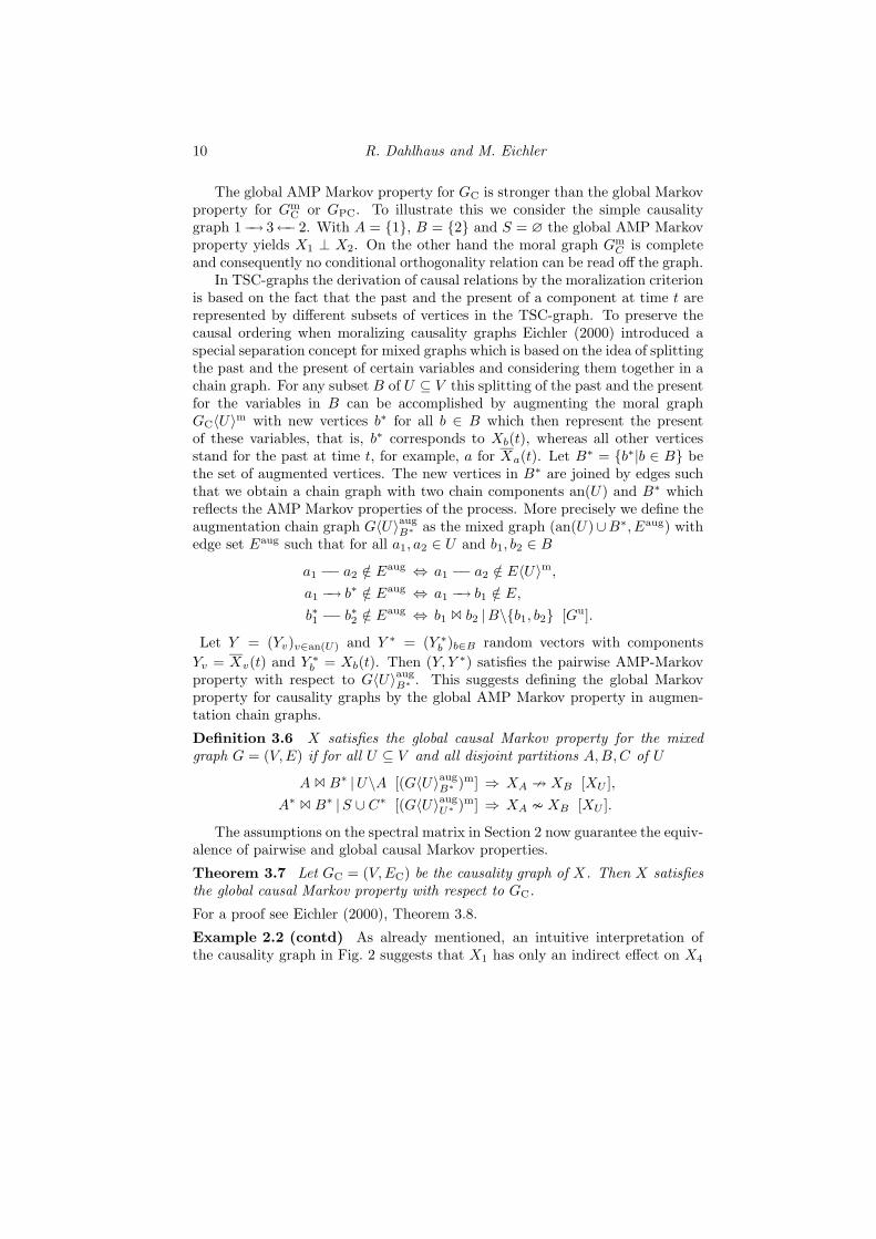
Fig. 5. Illustration of the global causal Markov property for the vectorautoregressive process in Example 2.2: (a) Augmentation chain graphG〈{1, 3, 4}〉aug

{4∗} and (b) its moral graph (G〈{1, 3, 4}〉aug{4∗})

m.

which is mediated by X3. That this interpretation is indeed correct can nowbe shown by deriving the relation X1 9 X4 [X{1,3,4}] from the correspondingaugmentation chain graph G〈{1, 3, 4}〉aug

{4∗}.Since the ancestral set generated by {1, 3, 4} is equal to the full set V we

start from the moral graph Gm in Fig. 3. Augmenting the graph with a newvertex 4∗ and joining this with vertex 4 and its parents 3 and 5 by arrowspointing towards 4∗ we obtain the augmentation chain graph G〈{1, 3, 4}〉aug

{4∗}in Fig. 5 (a). As the graph does not contain any flag or 2-biflag the removalof directions yields the moral graph (G〈{1, 3, 4}〉aug

{4∗})m in Fig. 5 (b). In this

graph the vertices 1 and 4∗ are separated by the set {3, 4} and hence the desirednoncausality relation follows from Theorem 3.7. Similarly it can be shown thatX1 and X4 are contemporaneously partially uncorrelated relative to the samesubprocess X{1,3,4} (Eichler 2000, Example 3.9)

3.4 The p-separation criterion

The moralization criterion in the previous sections is not a separation criterion inGTS of GC itself because the ancestral graphs and augmented moral graphs ap-pearing in the definitions of the global AMP and global causal Markov propertyvary with the subsets A, B, and S. For AMP chain graphs models Levitz et al.(2001) presented a pathwise separation criterion, called p-separation, which issimilar to the d-separation criterion for directed acyclic graphs. In Eichler (2001)it is shown that the global AMP Markov property and the global causal Markovproperty for causality graphs equivalently can be formulated by an adapted ver-sion of the p-separation criterion.

4 Inference for graphical time series models4.1 Conditional likelihood for graphical autoregressive models

We first discuss the case of fitting VAR(p) models restricted with respect to atime series chain graph. In practice the true TSC-graph is unknown and onehas to apply model selection strategies to find the best approximation for thetrue graph. Depending on the model discrepancy this leads to different modelselection criteria such as AIC or BIC. More precisely, let G = (VTS, E) be agraph from the class GTS(p) of all time series chain graphs whose edges haveat most lag p and which are invariant under translation in the sense that forall a, b ∈ V , and all t, s, u ∈ Z we have (a, t − u) −→ (b, t) /∈ E if and only if


(a, s− u)−→ (b, s) /∈ E and (a, t)−− (b, t) /∈ E if and only if (a, s)−− (b, s) /∈ E.We consider Gaussian VAR(p) models of the form

X(t) = A(1)X(t− 1) + . . .+A(p)X(t− p) + ε(t), ε(t) iid∼ N (0,ΣG)

where the parameters AG = (A(1), . . . , A(p)) and KG = Σ−1G satisfy the follow-

ing constraints

Aba(u) = 0 if (a, t)−→ (b, t+ u) /∈ E and Kab = 0 if (a, t)−− (b, t) /∈ E.

We call a vector autoregressive model with these constraints on the parametersa VAR(p,G) model.

Given observations X(1), . . . , X(T ) let T0 = T − p. The conditional loglikelihood function of a Gaussian VAR(p,G) model for the data can be writtenas (cf. Lutkepohl 1993)

LT

(AG,KG

)=d

2log(2π)− 1

2log |KG|+

12T0

T∑t=p+1

e(t)′KGe(t),

where e(t) = X(t) −∑pu=1A(u)X(t − u). Differentiating the log-likelihood we

obtain equations for the maximum likelihood estimate which can be solved nu-merically by an iterative algorithm (Dahlhaus and Eichler 2001). Furthermorewe can use model selection criteria for selection of the optimal VAR(p,G) modelamong all models with 1 ≤ p ≤ P and G ∈ GTS(p). Since in practice the numberof possible models is too large one has to use special model selection strategies.

Alternatively we can fit VAR(p) under the restrictions of a mixed graph Gfrom the class of all causality graphs GC. Such models are a special case of theVAR(p,G) models since by Proposition 2.5 for each G ∈ GC there exists a chaingraph G′ = (VTS, E

′) ∈ GTS(p) which implies exactly the same constraints onthe parameter as G, i.e. we have for all t ∈ Z (a, t) −− (b, t) /∈ E′ if and only ifa−− b /∈ E and (a, t)−→ (b, t+ u) /∈ E′ if and only if u > p or a−→ b /∈ E.

4.2 Partial directed and partial contemporaneous correlation

We now present a nonparametric approach for estimating TSC-graphs which isbased on the definition of the TSC-graphs itself. For random variables X, Y ,and Z let corrL(X,Y |Z) denote the correlation between X and Y after the lineareffects of Z have been removed. Thus we have corrL(X,Y |Z) = 0 if and only ifX ⊥ Y |Z. We define the partial directed correlation at lag u > 0 by

πba(u) = corrL

(Xb(t), Xa(t− u)

∣∣XV (t)\{Xa(t− u)})

and the partial contemporaneous correlation by

π◦ba = corrL

(Xb(t), Xa(t)

∣∣XV (t) ∪ {XV \{a,b}(t)}).


Then the time series chain graph GTS of a process X = {X(t)} can be charac-terized in terms of the partial directed and partial contemporaneous correlation,

(a, t− u)−→ (b, t) /∈ ETS ⇔ πba(u) 6= 0,(a, t)−− (b, t) /∈ ETS ⇔ π◦ba 6= 0.

When estimating the partial directed and partial contemporaneous correla-tions from observations X(1), . . . , X(T ) it is clear that only the observed partof the past can be taken into account. Therefore we define

πba(u) = corrL

(Xb(p), Xa(p− u)

∣∣{X(1), . . . , X(p− 1)}\{Xa(p− u)})

for some fixed p, with a similar definition for π◦ba. In Dahlhaus and Eichler (2001)an iterative scheme for the computation of these estimators has been suggested.

The estimators πba(u) and π◦ba can be used for testing for the existence of anedge in the TSC-graph GTS. More precisely, if the edge (a, t−u)−→(b, t) is absentin the true TSC-graph then T π2

ba(u) is asymptotically χ21-distributed. Similarly

we can test for the absence of undirected edges in the TSC-graph using thepartial contemporaneous correlation. For model selection these tests have to beapplied repeatedly for various edges which raises the usual problems associatedwith multiple testing.

In Proposition 2.5 we have seen that aggregation of the edges in the TSC-graph leads to the causality graph of the process. The idea of aggregation sug-gests to use the sum of π2

ba(u) for testing for the absence of a directed edge inthe causality graph. Let Rp being the empirical covariance matrix of X and H

a p×p matrix with entries Huv = (R−1p )bb(u−v)/(R−1

p )bb(0). Correcting for thedependence between the πba(u) at different lags we then obtain as a test statistic

Sab = T π′baH−1πba,

where πba is the vector of partial directed correlations. Under the null hypothesisthat Xa is noncausal for Xb the test statistic is asymptotically χ2

p-distributed.An equivalent test statistic has been presented by Tjøstheim (1982) for testingfor causality in multivariate time series (without considering causality relationsbetween the variables at the different time points themselves).

4.3 Partial correlation graphs

Inference for PC-graphs is in a certain sense more complicated than for TSC-graphs or causality graphs. Suppose for example that one wants to test by alikelihood ratio test the hypothesis that the edge a −− b is missing in the PC-graph of the VAR model in Example 2.2. This requires the calculation of themaximum likelihood estimator under the restrictions (2.4). There does not existan analytic solution for this problem whereas numerical solutions seem to bedifficult due to the particular nonlinear structure of the restrictions.

Instead we suggest a nonparametric method based on the characterization ofa missing edge by a vanishing partial spectral coherence in Proposition 2.7. By


0 6 12 18 24

0

10

20

30

40

50

60

70

80

time

conc

entr

atio

n

CO (100 µg/m³)NO (µg/m³)NO (µg/m³)2

�

ozone (µg/m³)radiation (10 W/m²)

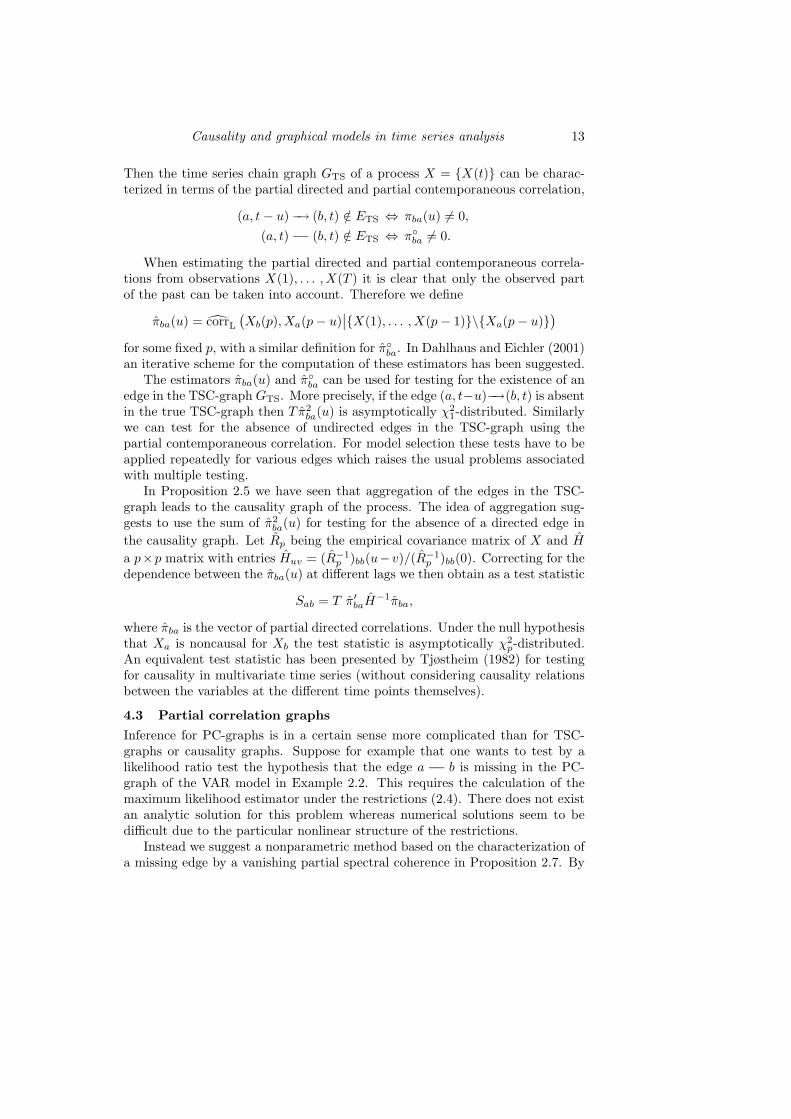
Fig. 6. Average of daily measurements over 61 days in summer.

this proposition the partial spectral coherence can be obtained by an inversionand rescaling of the spectral density matrix. We therefore estimate the spectralmatrix and invert and rescale this estimate. As an estimator for fab(λ) we takea kernel estimator based on the periodogram (cf. Dahlhaus, 2000).

We then test the hypothesis a −− b /∈ EPC by using an approximation ofthe distribution of supλ∈[−π,π] |Rab|V \{a,b}(λ)|2 under the hypothesis, i.e. underRab|V \{a,b}(λ) = 0 (for more details see Dahlhaus 2000, Section 5).

Alternatively the test can be based in the time domain on the partial corre-lations of Xa and Xb after removing the linear effects of XV \{a,b} (see Eichler etal. 2000).

5 ApplicationsIn order to illustrate the methods presented in this chapter we discuss two realdata example from chemistry and neurology. For further examples we refer toGather et al. (2002), who analyzed time series from intensive care monitoring bythe help of partial correlation graphs, and Eichler et al. (2000), who discussedthe identification of neural connectivities from spike train data.

5.1 Application to air pollution data

The method was used to analyze a 5-dimensional time series of length 35088of air pollutants recorded half-hourly from January 1991 to December 1992 inHeidelberg. The recorded variables were CO and NO (mainly emitted from cars,house-heating and industry), NO2 and O3 (created in different reactions in theatmosphere) and the global radiation intensity Irad which plays a major role inthe generation of ozone. Details on these reaction can be found e.g. in Seinfeld(1986, Chapter 4). Figure 6 shows the daily course of the five variables averagedover 61 successive days in summer. CO and NO increase early in the morningdue to traffic and, as a consequence, also NO2 increases. O3 increases later dueto the higher level of NO2 and the increase of the global radiation. Figure 6indicates that all variables are correlated at different lags.

The following analysis is based on the residual series after subtracting the(local) average course as shown in Fig. 6. The original series contained a fewmissing values (less than 2%) which were completed by interpolation of the


-1.0

1.0

-1.0

1.0

-1.0

1.0

-1.0

1.0

-6 0 6 -6 0 6 -6 0 6 -6 0 6

-1.0

1.0

-1.0

1.0

-1.0

1.0

-1.0

1.0

part

ial d

irect

ed/c

onte

mpo

rane

ous

corr

elat

ion

corr

elat

ion

time [h]

CO

NO

NO

O

I

2

3

rad

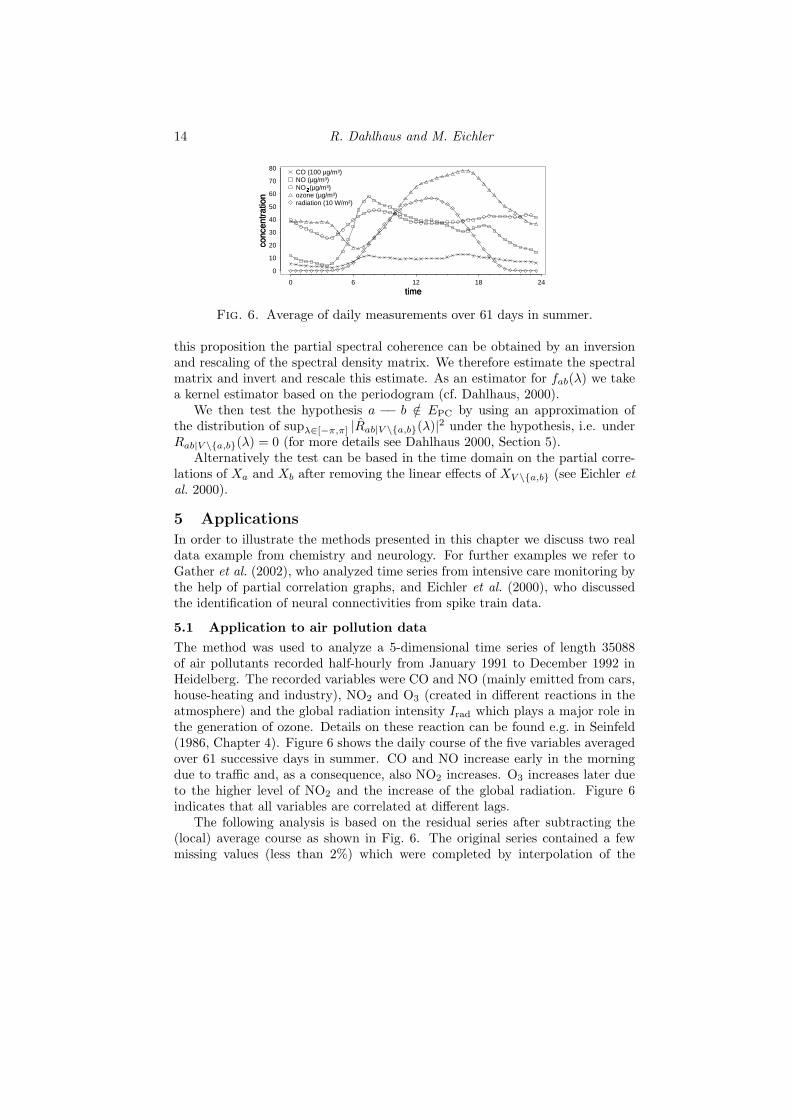
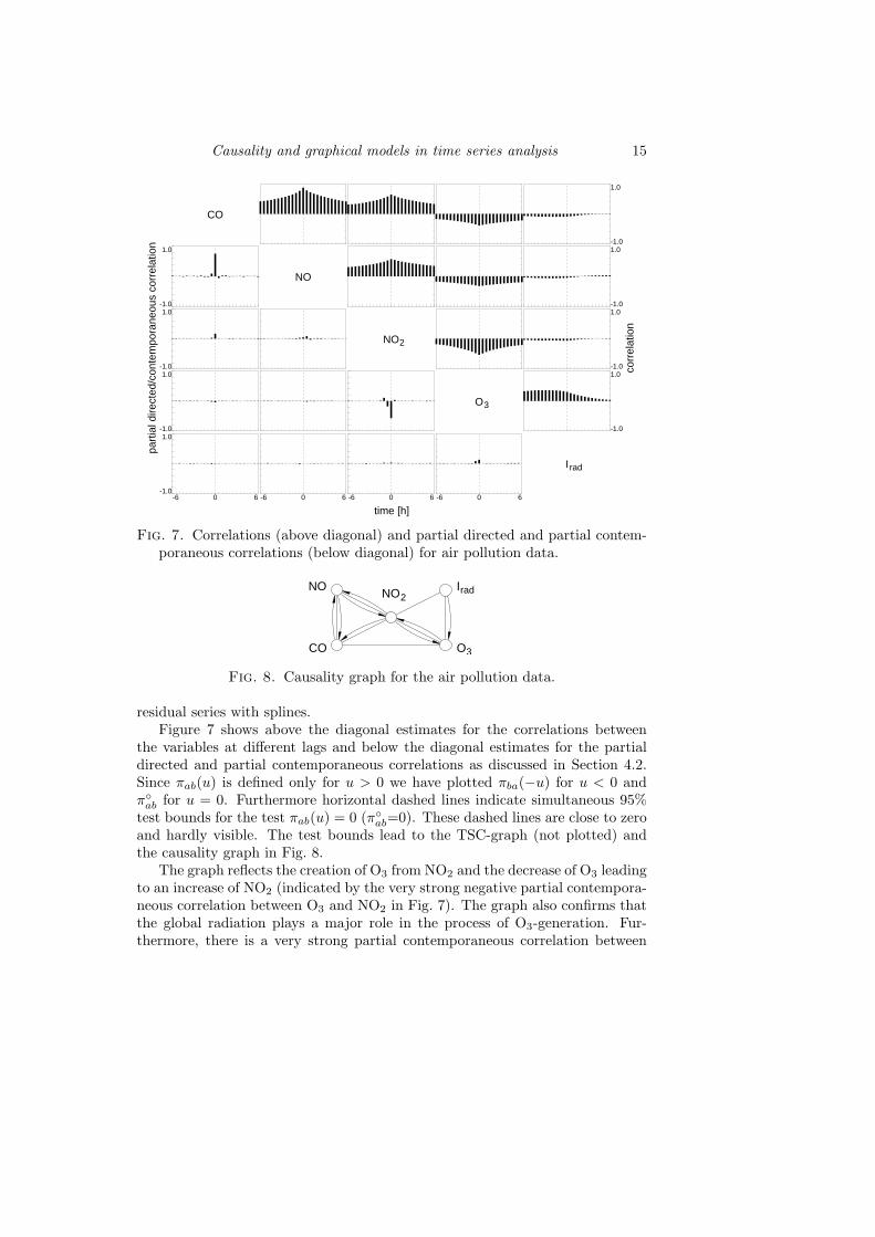
Fig. 7. Correlations (above diagonal) and partial directed and partial contem-poraneous correlations (below diagonal) for air pollution data.

I

O

rad

3CO

NONO2

Fig. 8. Causality graph for the air pollution data.

residual series with splines.Figure 7 shows above the diagonal estimates for the correlations between

the variables at different lags and below the diagonal estimates for the partialdirected and partial contemporaneous correlations as discussed in Section 4.2.Since πab(u) is defined only for u > 0 we have plotted πba(−u) for u < 0 andπ◦ab for u = 0. Furthermore horizontal dashed lines indicate simultaneous 95%test bounds for the test πab(u) = 0 (π◦ab=0). These dashed lines are close to zeroand hardly visible. The test bounds lead to the TSC-graph (not plotted) andthe causality graph in Fig. 8.

The graph reflects the creation of O3 from NO2 and the decrease of O3 leadingto an increase of NO2 (indicated by the very strong negative partial contempora-neous correlation between O3 and NO2 in Fig. 7). The graph also confirms thatthe global radiation plays a major role in the process of O3-generation. Fur-thermore, there is a very strong partial contemporaneous correlation between


CO and NO (both are emitted from cars etc.). The meaning of the other edges(and of some of the missing edges) is less obvious. Chemical reactions betweenair pollutants are very complex. In particular, one has to be aware of the factthat NO2 and O3 are not only increased but also decreased by several chemicalreactions and that several other chemicals play an important role.

Some of these reactions can be explained by a photochemical theory (cf. Se-infeld 1986, Section 4.2). This theory is confirmed by the above graph: First theedge between Irad and NO2 represents the photolysis of NO2. Second the edgesbetween NO and NO2 are present but Fig. 7 shows that the partial directedand partial contemporaneous correlations are less strong than the correlationbetween CO and NO2. This indicates that mainly the concentration of CO (andnot of NO) is responsible for the generation of NO2 which means that NO2 ismainly generated via a radical reaction (where CO is involved) and not in adirect reaction (where CO is not involved). This also is in accordance with thephotochemical theory for ozone generation.

The example shows the effect of the discretization interval (30 minutes) on thegraph. Obviously this interval is too large to resolve the direction in the chemicalreactions from the time flow. Thus most of the causality is detected as undirectedpartial contemporaneous correlation instead of directed Granger causality. Thereis one exception: The strong partial contemporaneous correlation between COand NO is due to the fact that both are emitted at the same time from cars,i.e. we have a confounder which is causal for both CO and NO.

The example also reveals the need for a more quantitative analysis in thatone wants to discriminate between major effects (such as NO2 −− O3 −− Irad)and minor effects (such as CO−−O3) leading to the idea of edges with differentgrey levels or colors reflecting the “strength” of a connection. This has to bepursued, in particular for applications with large data sets.

An analysis of the same data set discretized at a 4 hour interval with PC-graphs can be found in Dahlhaus (2000).

5.2 Application to human tremor data

The second example in this section is concerned with the identification of neu-rological signal transmission pathways in the investigation of human tremor.Tremor is defined as the involuntary, oscillatory movement of parts of the body,mainly the upper limbs. It has been shown that patients suffering from Parkin-son’s disease show a tremor-related cortical activity which can be detected inthe EEG time series by cross-spectral analysis (e.g. Timmer et al. 2000).

In one experiment the EEG and the surface electromyogram (EMG) of theleft hand wrist extensor muscle in a healthy subject have been measured duringan externally enforced oscillation of the hand with 1.9 Hz. The EMG signal wasband-pass filtered to avoid aliasing effects and undesired slow drifts. Additionallythe signal was digitally full wave rectified. The resulting time series reflects themuscle activity encoded in the envelope of the originally measured signal. TheEEG recordings were performed using a 64-channel EEG system. The potential


0.0

1.0

0.0

1.0

0 5 10 15 0 5 10 15

-2.0

6.0

0.0

8.0

6.0

12.0

0 5 10 15

-0.1

0.1

-0.1

0.1

-0.1

0.1

-30 0 30

part

ial d

irect

ed/c

onte

mpo

rane

ous

corr

elat

ion

part

ial c

oher

ence

/ lo

g sp

ectr

a

Frequency [Hz] Time [ms]

P1

C2P

Extensor

P1-C2P

P1-Extensor

C2P-Extensor

(b)(a)

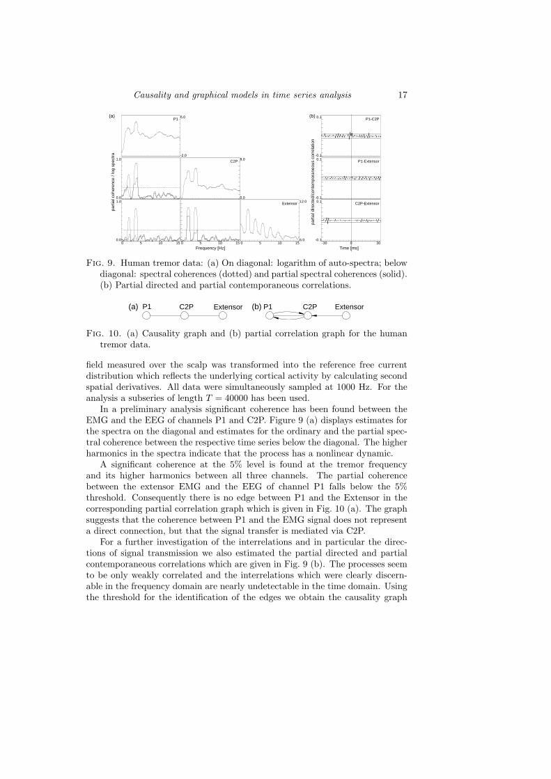
Fig. 9. Human tremor data: (a) On diagonal: logarithm of auto-spectra; belowdiagonal: spectral coherences (dotted) and partial spectral coherences (solid).(b) Partial directed and partial contemporaneous correlations.

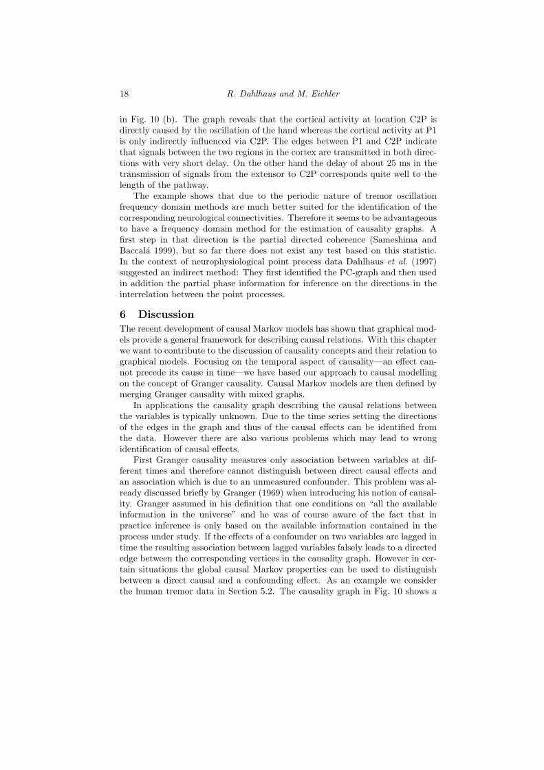
ExtensorP1 C2P C2P ExtensorP1(b)(a)

Fig. 10. (a) Causality graph and (b) partial correlation graph for the humantremor data.

field measured over the scalp was transformed into the reference free currentdistribution which reflects the underlying cortical activity by calculating secondspatial derivatives. All data were simultaneously sampled at 1000 Hz. For theanalysis a subseries of length T = 40000 has been used.

In a preliminary analysis significant coherence has been found between theEMG and the EEG of channels P1 and C2P. Figure 9 (a) displays estimates forthe spectra on the diagonal and estimates for the ordinary and the partial spec-tral coherence between the respective time series below the diagonal. The higherharmonics in the spectra indicate that the process has a nonlinear dynamic.

A significant coherence at the 5% level is found at the tremor frequencyand its higher harmonics between all three channels. The partial coherencebetween the extensor EMG and the EEG of channel P1 falls below the 5%threshold. Consequently there is no edge between P1 and the Extensor in thecorresponding partial correlation graph which is given in Fig. 10 (a). The graphsuggests that the coherence between P1 and the EMG signal does not representa direct connection, but that the signal transfer is mediated via C2P.

For a further investigation of the interrelations and in particular the direc-tions of signal transmission we also estimated the partial directed and partialcontemporaneous correlations which are given in Fig. 9 (b). The processes seemto be only weakly correlated and the interrelations which were clearly discern-able in the frequency domain are nearly undetectable in the time domain. Usingthe threshold for the identification of the edges we obtain the causality graph


in Fig. 10 (b). The graph reveals that the cortical activity at location C2P isdirectly caused by the oscillation of the hand whereas the cortical activity at P1is only indirectly influenced via C2P. The edges between P1 and C2P indicatethat signals between the two regions in the cortex are transmitted in both direc-tions with very short delay. On the other hand the delay of about 25 ms in thetransmission of signals from the extensor to C2P corresponds quite well to thelength of the pathway.

The example shows that due to the periodic nature of tremor oscillationfrequency domain methods are much better suited for the identification of thecorresponding neurological connectivities. Therefore it seems to be advantageousto have a frequency domain method for the estimation of causality graphs. Afirst step in that direction is the partial directed coherence (Sameshima andBaccala 1999), but so far there does not exist any test based on this statistic.In the context of neurophysiological point process data Dahlhaus et al. (1997)suggested an indirect method: They first identified the PC-graph and then usedin addition the partial phase information for inference on the directions in theinterrelation between the point processes.

6 DiscussionThe recent development of causal Markov models has shown that graphical mod-els provide a general framework for describing causal relations. With this chapterwe want to contribute to the discussion of causality concepts and their relation tographical models. Focusing on the temporal aspect of causality—an effect can-not precede its cause in time—we have based our approach to causal modellingon the concept of Granger causality. Causal Markov models are then defined bymerging Granger causality with mixed graphs.

In applications the causality graph describing the causal relations betweenthe variables is typically unknown. Due to the time series setting the directionsof the edges in the graph and thus of the causal effects can be identified fromthe data. However there are also various problems which may lead to wrongidentification of causal effects.

First Granger causality measures only association between variables at dif-ferent times and therefore cannot distinguish between direct causal effects andan association which is due to an unmeasured confounder. This problem was al-ready discussed briefly by Granger (1969) when introducing his notion of causal-ity. Granger assumed in his definition that one conditions on “all the availableinformation in the universe” and he was of course aware of the fact that inpractice inference is only based on the available information contained in theprocess under study. If the effects of a confounder on two variables are lagged intime the resulting association between lagged variables falsely leads to a directededge between the corresponding vertices in the causality graph. However in cer-tain situations the global causal Markov properties can be used to distinguishbetween a direct causal and a confounding effect. As an example we considerthe human tremor data in Section 5.2. The causality graph in Fig. 10 shows a


direct feedback between the two EEG channels P1 and C2P. The two channelsmight also be influenced by a third region in the brain. On the other hand abivariate analysis of P1 and the extensor shows that the latter is still causal forthe former. This contradicts the assumption of a confounder which would implythat the hand movements are noncausal for the cortical activity in channel P1.Therefore C2P must have a direct causal effect on P1 but we cannot excludethat part of the association is due to a confounder. For more details we refer toSection 4 of Eichler (2000).

Second, the identification of nonlinear causal effects is hampered by the re-striction to linear methods. Here, graphs defined in terms of conditional indepen-dence or strong Granger causality provide an alternative capturing the completedependence structure of the process. The results in Sections 2 and 3 also hold forthese graphs with one notable exception: The pairwise and the global Markovproperties for the TSC- and the causality graphs in general are no longer equiv-alent but only under additional assumption on the process. Alternatively thegraphs can be defined in terms of the so-called blockrecursive Markov propertieswhich are still equivalent to the global ones. For details we refer to Section 5 ofEichler (2000) and Eichler (2001). However, we mention that it is hardly pos-sible to make inference for arbitrary nonlinear causal relationships since strictlyspeaking we have only one observation of the multivariate process. This problemcould only be overcome by assuming specific nonlinear time series models.

A third limitation arises from the fact that the measured variables typicallyevolve continuously over time but are observed only at discrete times. If thetime between a cause and its effect is shorter than the sampling interval thenthe corresponding discretized component series are only contemporaneously cor-related and a directed edge is detected falsely as an undirected one. (We notethat contemporaneous causality may also be due to confounding by an unmea-sured process.) For the same reasons an indirect causality mediated by measuredvariables may lead to a directed edge in the causality graph.

The third problem can be avoided by replacing the discrete version of Grangercausality by local Granger causality and local instantaneous causality whichhave been introduced by Comte and Renault (1996) for the investigation ofcausal relations between time-continuous processes. We note that local Grangercausality is related to the notion of local independence (Schweder 1970; Aalen1987) which has been used by Didelez (2001) for the definition of directed graphsfor marked point processes.

Finally we note that the concept of Granger causality is not restricted tostationary time series but also applies to more general situations such as nonsta-tionary time series, panels of time series, or point processes. We conjecture thatthe graphical modelling approach can be applied in these cases in a similar way.

BibliographyAalen, O.O. (1987). Dynamic modelling and causality. Scandinavian ActuarialJournal, 177-190.


Aigner, D.J. and Zellner, A. (eds.) (1988). Causality. Journal of Econometrics,39, No.1/2, North Holland, Amsterdam, p. 1-234.Andersson, S.A., Madigan, D., and Perlman, M.D. (2001). Alternative Markovproperties for chain graphs. Scandinavian Journal of Statistics, 28, 33-85.Brillinger, D.R. (1981). Time Series: Data Analysis and Theory, McGraw Hill,New York.Comte, F. and Renault, E. (1996). Noncausality in continuous time models.Econometric Theory, 12, 215-256.Dahlhaus, R. (2000). Graphical interaction models for multivariate time series.Metrika, 51, 157-172.Dahlhaus, R., Eichler, M., and Sandkuhler, J. (1997). Identification of synapticconnections in neural ensembles by graphical models. Journal of NeuroscienceMethods, 77, 93-107.Dahlhaus, R. and Eichler, M. (2001). Statistical inference for time series chaingraphs. In preparation.Dawid, A.P. (2000). Causal inference without counterfactuals. Journal of theAmerican Statistical Association., 86, 9-26.Dempster, A.P. (1972). Covariance selection. Biometrics, 28, 157-175.Eichler, M. (1999). Graphical Models in Time Series Analysis. Doctoral thesis,University of Heidelberg, Germany.Eichler, M. (2000). Granger-causality graphs for multivariate time series. Tech-nical report, University of Heidelberg, Germany.Eichler, M. (2001). Markov properties for graphical time series models. Tech-nical report, University of Heidelberg, Germany.Eichler, M., Dahlhaus, R., and Sandkuhler, J. (2000). Partial correlation anal-ysis for the identification of synaptic connections. Technical report, Universityof Heidelberg, Germany.Frydenberg, M. (1990). The chain graph Markov property. Scandinavian Jour-nal of Statistics, 17, 333-353.Gather, U., Imhoff, M., and Fried, R. (2002). Graphical models for multi-variate time series from intensive care monitoring. Statistics in Medicine, toappear.Geweke, J. (1984). Inference and causality in economic time series. InZ. Griliches and M.D. Intriligator (eds.), Handbook of Econometrics, Vol. 2,North-Holland, Amsterdam, 1101-1144.Granger, C.W.J. (1969). Investigating causal relations by econometric modelsand cross-spectral methods. Econometrica, 37, 424-438.Haavelmo, T. (1943). The statistical implications of a system of simultaneousequations. Econometrica, 11, 1-12.Hsiao, C. (1982). Autoregressive modeling and causal ordering of econometricvariables. Journal of Economic Dynamics and Control, 4, 243-259.


Lauritzen, S.L. and Wermuth, N. (1989). Graphical models for associationbetween variables, some of which are qualitative and some are quantitative.Annals of Statistics, 17, 31-57.Lauritzen, S.L. (2000). Causal inference from graphical models. InE. Barndorff-Nielsen, D.R. Cox, and C. Kluppelberg (eds.) Complex StochasticSystems, CRC Press, LondonLevitz, M., Perlman, M.D., and Madigan, D. (2001). Separation and complete-ness properties for AMP chain graph markov models. Annals of Statistics, 29,1751 - 1784.Lutkepohl, H. (1993). Introduction to multiple time series analysis. Springer,Berlin.Lynggaard, H., and Walther, K.H. (1993). Dynamic Modelling with MixedGraphical Association Models. Master’s Thesis, Aalborg University.Neyman, J. (1923). Statistical problems in agricultural experimentation (withdiscussion). Journal of the Royal Statistical Society Suppl., 2, 107-180.Pearl, J. (1988). Probabilistic Inference in Intelligent Systems. Morgan Kauf-mann, San Mateo, California.Pearl, J. (1995). Causal diagrams for empirical research (with discussion).Biometrika, 82, 669-710.Pearl, J. (2000). Causality, Cambridge University Press, Cambridge, UK.Robins, J. (1986). A new approach to causal inference in mortality studieswith sustained exposure periods - application to control of the healthy workersurvivor effect. Mathematical Modelling, 7, 1393-1512.Rubin, D.B. (1974). Estimating causal effects of treatments in randomizedand nonrandomized studies. Journal of Educational Psychology, 66, 688-701.Sameshima, K. and Baccala, L.A. (1999). Using partial directed coherence todescribe neuronal ensemble interactions. Journal of Neuroscience Methods, 94,93-103.Schweder, T. (1970). Composable Markov processes. Journal of Applied Prob-ability, 7, 400-410.Seinfeld, J.H. (1986). Atmospheric Chemistry and Physics of Air Pollution.John Wiley, Chichester.Timmer, J., Lauk, M., Koster, B., Hellwig, B., Haußler, S., Guschlbauer, B.,Radt, V., Eichler, M., Deuschl, G., and Lucking, C.H. (2000). Cross-spectralanalysis of tremor time series. Int. J. of Bifurcation and Chaos, 10, 2595-2610.Tjøstheim, D. (1981). Granger-causality in multiple time series. Journal ofEconometrics, 17, 157-176.Wright, S. (1921). Correlation and causation. Journal of Agricultural Research,20, 557-585.

causality and graphical models in time series analysisgalton.uchicago.edu/~eichler/hsss.pdf · 1...

Documents