causal inference with observational data - boston collegefm · causal inference with observational...

OverviewPanel Methods

Matching and ReweightingInstrumental Variables (IV)

Regression Discontinuity (RD)More

Causal inference with observational dataRegression Discontinuity and related methods in Stata

Austin Nichols

June 26, 2009

Austin Nichols Causal inference with observational data




Selection and EndogeneityThe Gold Standard

Selection and Endogeneity

In a model like y = Xb + e, we must have E(X ′e) = 0 for unbiased estimatesof b. This assumption fails in the presence of measurement error, simultaneousequations, omitted variables in X , or selection (of X ) based on unobserved orunobservable factors. The “selection problem” is my focus.

A classic example is the effect of education on earnings, where the highestability individuals may get more education, but would have had higher earningsregardless (leading us under this simple assumption to guess that the effect ofeducation is overestimated). The selection problem can often be framed as acase of omitted variables (e.g. ability) or misspecification, but is more general.

Solution: observe unobserved factors, or attempt to control for unobservablefactors, using an experiment and/or quasi-experimental (QE) methods.Though I focus on the selection problem and QE methods, they are also usedfor other cases of endogeneity listed above; see e.g. Hardin, Schmiediche, andCarroll (2003) on measurement error.


http://www.stata.com/merror/





A Simple Example

-------------------------------------------------------

| Success

Treatment | 0 1 Total

----------+--------------------------------------------

P | .1743 .8257 1

| [.1621,.1872] [.8128,.8379]

|

O | .22 .78 1

| [.2066,.234] [.766,.7934]

|

Total | .1971 .8029 1

| [.188,.2066] [.7934,.812]

-------------------------------------------------------

Key: row proportions

[95% confidence intervals for row proportions]






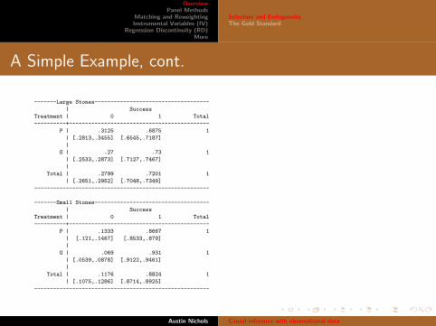
A Simple Example, cont.

-------Large Stones------------------------------------

| Success


----------+--------------------------------------------

P | .3125 .6875 1

| [.2813,.3455] [.6545,.7187]

|

O | .27 .73 1

| [.2533,.2873] [.7127,.7467]

|

Total | .2799 .7201 1

| [.2651,.2952] [.7048,.7349]

-------------------------------------------------------

-------Small Stones------------------------------------

| Success


----------+--------------------------------------------

P | .1333 .8667 1

| [.121,.1467] [.8533,.879]

|

O | .069 .931 1

| [.0539,.0878] [.9122,.9461]

|

Total | .1176 .8824 1

| [.1075,.1286] [.8714,.8925]

-------------------------------------------------------






The Rubin Causal Model

Rubin (1974) gave us the model of identification of causal effects that mosteconometricians carry around in their heads, which relies on the notion of ahypothetical counterfactual for each observation. The model flows from workby Neyman (1923,1935) and Fisher (1915,1925), and perhaps the clearestexposition is by Holland (1986); see also Tukey (1954), Wold (1956), Cochran(1965), Pearl (2000), and Rosenbaum (2002).

To estimate the effect of a college degree on earnings, we’d like to observe theearnings of college graduates had they not gone to college, to compute the gainin earnings, and to observe the earnings of nongraduates had they gone tocollege, to compute their potential gain in earnings.

One method here is to call the missing information on hypotheticalcounterfactual outcomes missing data, and to impute the missing data—this isessentially the approach a matching estimator takes. The other leading QEcandidates are panel methods, reweighting techniques, instrumental variables(IV), and regression discontinuity (RD) approaches.






The Fundamental Problem

The Fundamental Problem is that we can never see the counterfactualoutcome, but randomization of treatment lets us estimate treatment effects. Tomake matters concrete, imagine the treatment effect is the same for everyonebut there is heterogeneity in levels—suppose there are two types 1 and 2:

Type E [y |T ] E [y |C ] TE

1 100 50 502 70 20 50

and the problem is that the treatment T is not applied with equal probabilityto each type. For simplicity, suppose only type 1 gets treatment T and put amissing dot in where we cannot compute a sample mean:


1 100 . ?2 . 20 ?

The difference in sample means overestimates the ATE (80 instead of 50); ifonly type 2 gets treatment the difference in sample means underestimates theATE (20 instead of 50).






The Solution

Random assignment puts equal weight on each of the possible observedoutcomes:


1 100 . ?2 . 20 ?1 . 50 ?2 70 . ?

and the difference in sample means is an unbiased estimate of the ATE.






The Gold Standard Solution

To control for unobservable factors, the universally preferred method is arandomized controlled trial, where individuals are assigned X randomly. In thesimplest case of binary X , where X = 1 is the treatment group and X = 0 thecontrol, the effect of X is a simple difference in means, and all unobserved andunobservable selection problems are avoided. In fact, we can always do better(Fisher 1926) by conditioning on observables, or running a regression on morethan just a treatment dummy, as the multiple comparisons improve efficiency.

In many cases, an RCT is infeasible due to cost or legal/moral objections.Apparently, you can’t randomly assign people to smoke cigarettes or not. Youalso can’t randomly assign different types of parents or a new marital status,either. Without random assignment, we have observational data, and anobservational study. Methods for consistently estimating b in observationaldata are quasi-experimental methods, and include no method at all (i.e. yourun the same regression you would have before you realized there might be aselection problem). Angrist and Pischke (2009) provide a good overview of afew approaches, and Imbens and Wooldridge (2007) cover most.






All That Glitters

Even where an experiment is feasible, the implementation can be quitedaunting. Often, the individuals who are randomly assigned will agitate to bein another group—the controls want to get treatment if they perceive abenefit, or the treatment group wants to drop out if the treatment feelsonerous—or behave differently.

Even in a double-blind RCT, there may be leakage between treatment andcontrol groups, or differing behavioral responses. Those getting a placebo mayself-medicate in ways the treatment group do not (imagine a double-blind RCTfor treatment of heroin addiction), or side effects of treatment may induce thetreatment group to take some set of actions different from the control group (ifyour pills made you too sick to work, you might either stop taking the pills orstop working—presumably the placebo induces fewer people to give up work).






QE Methods in Experiments

In practice, all of the quasi-experimental methods here are used in experimentalsettings as well as in observational studies, to attempt to control for departuresfrom the ideal of the RCT.

Sometimes, the folks designing experiments are clever and build in comparisonsof the RCT approach and observational approaches. See Orr et al. (1996) forone example where OLS appears to outperform the more sophisticatedalternatives, and Heckman, Ichimura, and Todd (1997) where moresophisticated alternatives are preferred. Smith and Todd (2001,2005) pursuethese comparisons further.

Another major problem with experiments is that they tend to use small andselect populations, so that an unbiased estimate of a treatment effect isavailable only for a subpopulation, and the estimate may have large variance.This is mostly a question of scale, but highlights the cost, bias, and efficiencytradeoffs in choosing between an experiment and an observational study.






Treatment Effect

Just to be clear:

The “treatment effects” literature usually focuses on a binary indicator fortreatment where X = 1 indicates the treatment group and X = 0 the control,but X is not randomly assigned in the sample.

I will use the term “treatment” for any potentially endogenous variable in Xwhose effect we wish to measure, including continuous variables. Manytreatments come in different types or intensities, and we often estimate theeffect of a one-unit increase in intensity, however intensity happens to bemeasured.






The Counterfactual Again

The mention of the placebo group self-medicating may also bring to mind whathappens in social experiments. If some folks are assigned to the control group,does that mean they get no treatment? Generally not. A person who isassigned to get no job training as part of an experiment may get someelsewhere. Someone assigned to get job training as part of an experiment maysleep through it.

The treatment group may not get treated; the control group may not gountreated. The important thing to bear in mind is the relevantcounterfactual: what two regimes are you comparing? A world in whicheveryone who gets treated gets the maximum intensity treatment perfectlyapplied, and those who don’t get treated sit in an empty room and do nothing?What is the status quo for those not treated?





Diff-in-Diff and Natural ExperimentsDifference and Fixed Effects ModelsMore ModelsATE and LATE

DD

The most basic quasi-experimental method used in observational studies isidentical to that used in most RCT’s, the difference in differences (DD)method.

Pre Post ATETreatment y1 y2 (y2 − y1)− (y4 − y3)Control y3 y4

The average treatment effect (ATE) estimate is the difference in differences.For example, the estimate might be the test score gain from 8th grade to 12thgrade for those attending charter schools less the test score gain for those inregular public schools. This assumes that the kids in charters, who had toapply to get in, would not have had the same gains in a regular school, i.e.that there was no selection into treatment.






DD, DDD, Dn

Having differenced out the “time” effect or the “state” effect, it is natural towant to add dimensions and compute a difference in differences in differences,and so on. This is equivalent to adding indicator variables and interactions to aregression, and the usual concerns apply to the added variables.

The usual “good” diff-in-diff approach relies on a natural experiment, i.e. therewas some change in policy or the environment expected to affect treatment forone group more than another, and the two groups should not otherwise havedifferent experiences. For this to work well, the natural experiment should beexogenous itself (i.e. it should not be the case that the policy change is areaction to behavior) and unlikely to induce people to “game the system” andchange their behavior in unpredictable ways.






A Natural Experiment Example

For example, in some US states in 1996, immigrants became ineligible for foodstamps, but 17 states offered a substitute program for those in the countrybefore 1996. As of July 2002, anyone in the country five years was eligible forfood stamps and most of those in the country 4.9 years were not. One couldcompute a difference in mean outcomes (say, prevalence of obesity) acrossrecent and less recent immigrants, across calendar years 1995 and 1996, acrossaffected and unaffected states. Using 2002, you could compute a differenceacross the population of immigrants in the country 4 years or 5 years. SeeKaushal (2007) for a related approach.






Good Natural Experiments

In most cases, these types of natural experiments call for one of the othermethods below (the food stamp example cries out for an RegressionDiscontinuity approach using individual data). A hybrid of DD and anotherapproach is often best.

In general, the more bizarre and byzantine the rules changes, and the moredraconian the change, the more likely a natural experiment is likely to identifysome effect of interest. A modest change in marginal tax rates may not providesufficient power to identify any interesting behavioral parameters, but the topmarginal estate tax rates falling from 45% in 2009 to zero in 2010 and thenjumping to 55% in 2011 creates an interesting incentive for mercenary childrento pull the plug on rich parents in the tax-free year.






Difference and Fixed Effects Models

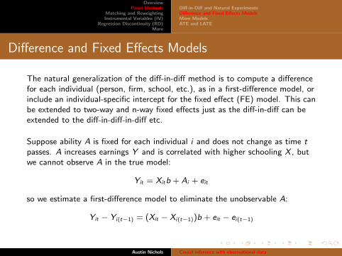
The natural generalization of the diff-in-diff method is to compute a differencefor each individual (person, firm, school, etc.), as in a first-difference model, orinclude an individual-specific intercept for the fixed effect (FE) model. This canbe extended to two-way and n-way fixed effects just as the diff-in-diff can beextended to the diff-in-diff-in-diff etc.

Suppose ability A is fixed for each individual i and does not change as time tpasses. A increases earnings Y and is correlated with higher schooling X , butwe cannot observe A in the true model:

Yit = Xitb + Ai + eit

so we estimate a first-difference model to eliminate the unobservable A:

Yit − Yi(t−1) = (Xit − Xi(t−1))b + eit − ei(t−1)






Fixed Effects Models

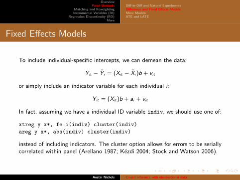
To include individual-specific intercepts, we can demean the data:

Yit − Yi = (Xit − Xi )b + vit

or simply include an indicator variable for each individual i :

Yit = (Xit)b + ai + vit

In fact, assuming we have a individual ID variable indiv, we should use one of:

xtreg y x*, fe i(indiv) cluster(indiv)

areg y x*, abs(indiv) cluster(indiv)

instead of including indicators. The cluster option allows for errors to be seriallycorrelated within panel (Arellano 1987; Kezdi 2004; Stock and Watson 2006).






2-way Fixed Effects Models

Including additional sets of fixed effects, as for time periods, is easiest viaindicator variables:

qui tab year, gen(iy)drop iy1areg y x* iy*, abs(indiv) cluster(indiv)

See Abowd, Creecy, and Kramarz (2002) and Andrews, Schank, andUpward (2005) for faster estimation of n-way fixed effects. See alsoCameron, Gelbach, and Miller (2006) for two-way clustering of errors,and Cameron, Gelbach, and Miller (2007) for a bootstrap approach toestimating cluster-robust standard errors with fewer than 50 clusters.






First Difference, Fixed Effects, and Long Difference0

.51

1.5

Pre Post






First Difference, Fixed Effects, and Long Difference

FD=.50.5

11.

5

Pre Post







FE=1

FD=.50.5

11.

5

Pre Post







FE=1

FD=.5

LD=1.2

0.5

11.

5

Pre Post






FD, FE, and LD

Clearly, one must impose some assumptions on the speed with which Xaffects Y , or have some evidence as to the right time frame forestimation. This type of choice comes up frequently when stock pricesare supposed to have adjusted to some news, especially given thefrequency of data available—economists believe the new information iscapitalized in prices, but not instantaneously. Taking a difference in stockprices between 3:01pm and 3pm is inappropriate, but taking a longdifference over a year is clearly inappropriate as well, since newinformation arrives continuously.

One should always think about within-panel trends and the frequency ofmeasurement. Baum (2006) discussed some filtering techniques to getdifferent frequency “signals” from noisy data. Personally, I like a simplemethod due to Baker, Benjamin, and Stanger (1999).






Growth Models

In the food stamps example, if you had daily observations on height andweight, you would not want to estimate the one-day change in obesityamong the affected group. Similarly, for an educational intervention, thetest scores on the second day are probably not the best measure, but arethe test scores on the last day? In the Tennessee STAR experiment, somestudents were placed in smaller classes, and had higher test scores at theend of the year. If they don’t have higher test scores after five years,should we care?






There is a large class of growth models, where the effect of X is assumed to beon the rate of change in Y . The natural way to specify these models is toinclude an elapsed time variable and interact it with X .

Yit = Xitb + Titg + TXit f + Ai + eit

For a binary X, the marginal effect of X for each observation is then b + fTit

(or b[x]+ b[timex]*time in Stata with T variable time and TX variabletimex), and we can imagine taking the mean across relevant time periods orcomputing this quantity at some specified end point, i.e. we are back tochoosing among first difference or long difference models.

In practice, growth models are usually estimated using hierarchical models,such as xtmixed, xtmelogit, xtmepoisson or some form of gllamm model(Rabe-Hesketh, Skrondal, and Pickles 2002).






Consistency

Note the assumption I started with: Suppose ability A is fixed for eachindividual i but does not change as time t passes. If ability doesn’tchange over time, what is the point of education? A facile observation,perhaps, but the point is that the assumed selection was of the mostuncomplicated variety, and it is natural to think that people differ inunobservable ways over time as well.

If people differ in unobservable ways over time as well, or selection ismore complicated, these panel methods will not provide consistentestimates of the effect b.






Other Panel Models

There are a variety of random effect and GLS methods that exploitdistributional assumptions to estimate more complicated panel models,and there is the random coefficient case

Yit = Xitbi + eit

which seems like a natural extension to the basic panel setting (see xtrcin Stata 10). With more assumptions come more violations ofassumptions, but greater efficiency (and potentially less bias) if theassumptions hold.






ATE

The mention of individual-specific coefficients raises the question of whatexactly we wish to estimate. If individuals may have different treatmenteffects, or marginal effects, of some endogenous X, a regression of Y onX will not in general recover the mean marginal effect of X, or averagetreatment effect (ATE).






OLS inconsistent for ATE

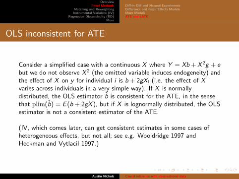
Consider a simplified case with a continuous X where Y = Xb + X 2g + ebut we do not observe X 2 (the omitted variable induces endogeneity) andthe effect of X on y for individual i is b + 2gXi (i.e. the effect of Xvaries across individuals in a very simple way). If X is normallydistributed, the OLS estimator b is consistent for the ATE, in the sensethat plim(b) = E (b + 2gX ), but if X is lognormally distributed, the OLSestimator is not a consistent estimator of the ATE.

(IV, which comes later, can get consistent estimates in some cases ofheterogeneous effects, but not all; see e.g. Wooldridge 1997 andHeckman and Vytlacil 1997.)






ATE and LATE

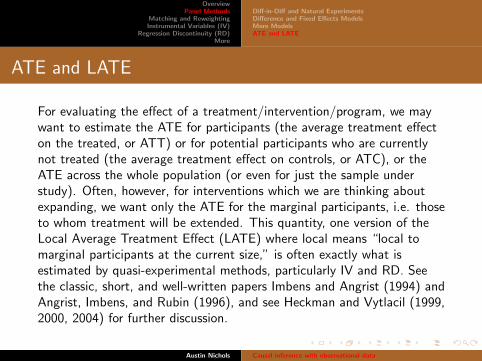
For evaluating the effect of a treatment/intervention/program, we maywant to estimate the ATE for participants (the average treatment effecton the treated, or ATT) or for potential participants who are currentlynot treated (the average treatment effect on controls, or ATC), or theATE across the whole population (or even for just the sample understudy). Often, however, for interventions which we are thinking aboutexpanding, we want only the ATE for the marginal participants, i.e. thoseto whom treatment will be extended. This quantity, one version of theLocal Average Treatment Effect (LATE) where local means “local tomarginal participants at the current size,” is often exactly what isestimated by quasi-experimental methods, particularly IV and RD. Seethe classic, short, and well-written papers Imbens and Angrist (1994) andAngrist, Imbens, and Rubin (1996), and see Heckman and Vytlacil (1999,2000, 2004) for further discussion.






Outline

OverviewSelection and EndogeneityThe Gold Standard

Panel MethodsDiff-in-Diff and Natural ExperimentsDifference and Fixed Effects ModelsMore ModelsATE and LATE

Matching and ReweightingNearest Neighbor MatchingPropensity score matchingReweighting

Instrumental Variables (IV)Forms of IVNecessary Specification TestsGeneralizations using Control FunctionsThe zeroth stageTreatreg

Regression Discontinuity (RD)Deterministic or Probabilistic AssignmentInterpretationRD Modeling ChoicesSpecification Testing

MoreSensitivity TestingConnections across method typesConclusionsReferences





Nearest Neighbor MatchingPropensity score matchingReweighting

Outline












Matching and Reweighting Distributions

If individuals in the treatment and control groups differ in observableways (selection on observables case), a variety of estimators are possible.One may be able to include indicators and interactions for the factorsthat affect selection, to estimate the impact of some treatment variablewithin groups of identical X (a fully saturated regression). There are alsomatching estimators (Cochran and Rubin 1973) which compareobservations with like X , for example by pairing observations that are“close” by some metric. A set of alternative approaches involvereweighting so the distribution of X is identical for different groups,discussed in Nichols (2008).






Nearest Neighbor Matching

Nearest neighbor matching pairs observations in the treatment andcontrol groups and computes the difference in outcome Y for each pair,then the mean difference across pairs. Imbens (2006) presented at lastyear’s meetings on the Stata implementation nnmatch (Abadie et al.2004). See Imbens (2004) for details of Nearest Neighbor Matchingmethods.

The downside to Nearest Neighbor Matching is that it can becomputationally intensive, and bootstrapped standard errors are infeasibleowning to the discontinuous nature of matching (Abadie and Imbens,2006).






Propensity score matching

Propensity score matching essentially estimates each individual’spropensity to receive a binary treatment (via a probit or logit) as afunction of observables and matches individuals with similar propensities.As Rosenbaum and Rubin (1983) showed, if the propensity were knownfor each case, it would incorporate all the information about selection andpropensity score matching could achieve optimal efficiency andconsistency; in practice, the propensity must be estimated and selectionis not only on observables, so the estimator will be both biased andinefficient.

Morgan and Harding (2006) provide an excellent overview of practicaland theoretical issues in matching, and comparisons of nearest neighbormatching and propensity score matching. Their expositions of differenttypes of propensity score matching, and simulations showing when itperforms badly, are particularly helpful.






Propensity score matching methods

Typically, one treatment case is matched to several control cases, butone-to-one matching is also common. One Stata implementation psmatch2 isavailable from SSC (ssc desc psmatch2) and has a useful help file, and thereis another Stata implementation described by Becker and Ichino (2002)(findit pscore in Stata). psmatch2 will perform one-to-one (nearestneighbour or within caliper, with or without replacement), k-nearest neighbors,radius, kernel, local linear regression, and Mahalanobis matching.

As Morgan and Harding (2006) point out, all the matching estimators can bethought of as reweighting scheme whereby treatment and control observationsare reweighted to allow causal inference on the difference in means. Note thata treatment case i matched to k cases in an interval, or k nearest neighbors,contributes yi − k−1 ∑k

1 yj to the estimate of a treatment effect, and one couldjust as easily rewrite the estimate of a treatment effect as a weighted meandifference.






Common support

Propensity score methods typically assume a common support, i.e. the range ofpropensities to be treated is the same for treated and control cases, even if thedensity functions have quite different shapes. In practice, it is rarely the casethat the ranges of estimated propensity scores are the same, but they do nearlyalways overlap, and generalizations about treatment effects should probably belimited to the smallest connected area of common support.

Often a density estimate below some threshold greater than zero defines theend of common support—see Heckman, Ichimura, and Todd (1997) for morediscussion. This is because the common support is the range where bothdensities are nonzero, but the estimated propensity scores take on a finitenumber of values, so the empirical densities will be zero almosteverywhere—we need a kernel density estimate in general, to obtain smoothestimated density functions, but then areas of zero density may have positivedensity estimates, so some small value is redefined to be effectively zero.






Common support diagnostic graph

It is unappealing to limit the sample to a range of estimated propensity scores, since itis hard to characterize the population to which an estimate would generalize in thatcase. A more appealing choice if the distributions of propensity scores exhibit pooroverlap, or if kernel density estimates of propensity scores for treatment or controlgroups exhibit positive density or nonzero slope at zero or one, is to limit to ranges ofX variables, such that the distributions of propensity scores exhibit better properties.At least in this case, we can say “our estimates apply to unemployed native workerswith less than a college education” or somesuch, together with an acknowledgementthat we would like estimates for the population as well, but the method employed didnot allow it.

Regardless of whether the estimation or extrapolation of estimates is limited to arange of propensities or ranges of X variables, the analyst should present evidence onhow the treatment and control groups differ, and which subpopulation is beingstudied. The standard graph here is an overlay of kernel density estimates ofpropensity scores for treatment and control groups, easy in Stata with twoway

kdensity (but better with akdensity or kdens on SSC; the latter allows a boundarycorrection at zero and one). DiNardo and Tobias (2001) provide an overview ofnonparametric estimators including kernel density estimators.






Propensity score reweighting

The propensity score can also be used to reweight the treatment and controlgroups so the distribution of X looks the same in both groups: one method isto give treatment cases weight one and control cases weight p/(1− p) where pis the probability of treatment. Additional choices are discussed in Nichols(2008).

Note that the assumption that p is bounded away from zero and one isimportant here. If estimated p approaches one for a control case, thereweighting scheme above assigns infinite weight to one control case as thecounterfactual for every treatment case, and this control case should not evenexist (as p approaches one for a control case, the probability of observing sucha case approaches zero)!






Propensity scores, true and estimated

Part of the problem may be that propensity scores are estimated. If we had truepropensity scores, they would certainly never be one for a control case. But it turnsout that is really not the problem, at least for mean squared error in estimates ofcausal impacts. In fact, you can usually do better using an estimated propensity score,even with specification error in the propensity score model, than using the truepropensity score (based on unpublished simulations). This arises because the varianceof estimates using true propensity scores is very high, whereas using an estimatedpropensity score is effectively a shrinkage estimator, which greatly reduces meansquared error.

In fact, Hirano, Imbens, and Ridder (2003) show that using nonparametric estimatesof the propensity score to construct weights is efficient relative to using truepropensity scores or covariates, and achieves the theoretical bound on efficiency (butsee Song 2009 for a case where this does not hold).

It is a problem that propensity scores are estimated, because that fact is not used inconstructing standard errors, so most SEs are too small in some sense. Yet if we thinkthat using estimated propensity scores and throwing away information on truepropensity scores can improve efficiency, perhaps our standard errors are actually toolarge! This is an active research area, but most people will construct standard errorsassuming no error in estimated propensity scores.






More reweighting

The large set of reweighting techniques lead to a whole class of estimatorsbased on reweighting the treatment and control groups to have similardistributions of X in a regression. The reweighting techniques include DiNardo,Fortin, and Lemieux (1996), Autor, Katz, and Kearney (2005), Liebbrandt,Levinsohn, and McCrary (2005), and Machado and Mata(2005), and arerelated to decomposition techniques in Blinder (1973), Oaxaca (1973), Yun(2004, 2005ab), Gomulka and Stern (1990), and Juhn, Murphy, and Pierce(1991, 1993).

DiNardo (2002) draws some very useful connections between thedecomposition and reweighting techniques, and propensity score methods, buta comprehensive review is needed.






Selection on unobservables etc.

Imagine the outcome is wage and the treatment variable is union membership—onecan imagine reweighting union members to have equivalent education, age,race/ethnicity, and other job and demographic characteristics as nonunion workers.One could compare otherwise identical persons within occupation and industry cellsusing nnmatch with exact matching on some characteristics. The various propensityscore methods offer various middle roads.

However, these estimates based on reweighting or matching are unlikely to convincesomeone unconvinced by OLS results. Selection on observables is not the type ofselection most critics have in mind, and there are a variety of remaining problemsunaddressed by reweighting or matching, such as selection into a pool eligible forassignment to treatment or control—e.g. in the union case, there may be differentiallabor market participation (so whether or not a particular person would be in a union isunknown for many cases). One hypothesized effect of unions is a reduction in the sizeof workforces—if unionized jobs produce different proportions working, the marginalworker is from a different part of the distribution in the two populations. DiNardo andLee (2002) offer a much more convincing set of causal estimates using an RD design.





Forms of IVNecessary Specification TestsGeneralizations using Control FunctionsThe zeroth stageTreatreg

Outline












IV methods

The idea of IV is to exploit another moment condition E(Z ′e) = 0 when we thinkE(X ′e) 6= 0. Put another way, Z moves X around in such a way that there is someexogenous variation in X we can use to estimate the causal effect of X on Y . It is thisway of characterizing IV that leads people to think they are getting an unbiasedestimator, but it is worthwhile to remember the IV estimator is biased but consistent,and has substantially lower efficiency than OLS. Thus, if a significant OLS estimate b

becomes an insignificant bIV when using IV, one cannot immediately conclude thatb = 0. Failure to reject the null should not lead you to accept it.

There are a variety of things that can go wrong in IV, particularly if your chosenexcluded instruments don’t satisfy E(Z ′e) = 0 or if Z is only weakly correlated withthe endogenous X . You should always test for endogeneity of your supposedlyendogenous variable, and test that your IV estimate differs from your OLS pointestimate (not just from zero). You should also conduct overidentification tests andidentification tests, and tests for weak instruments. Luckily, all of the tests are easilydone in Stata, and some are part of official Stata as of release 10.






Forms of IV

I The IV Estimator The instrumental variables estimator in ivreg is a one-step estimator thatcan be thought of as equivalent to a variety of 2-step estimators; most think of it as aprojection of y on the projection of X on Z .

I Two-stage Least Squares (2SLS) is an instrumental variables estimation technique that isformally equivalent to the one-step estimator in the linear case. First, use OLS to regress Xon Z and get X = Z(Z ′Z)−1Z ′X , thenS use OLS to regress y on X to get βIV .

I Ratio of Coefficients: If you have one endogenous variable X and one instrument Z , you canregress X on Z to get π = (Z ′Z)−1Z ′X and regress y on Z to get γ = (Z ′Z)−1Z ′y , and

the IV estimate βIV = γ/π. If X is a binary indicator variable, this ratio of coefficientsmethod is known as the Wald estimator.

I The Control Function Approach: The most useful approach considers another set of twostages: use OLS to regress X on Z and get estimated errors ν = X − Z(Z ′Z)−1Z ′X then

use OLS to regress y on X and ν to get βIV .

Note that in every case the set of excluded instruments does not vary; if different instruments areto be used for different endogenous variables, you have a system estimator and should use reg3(and read Goldberger and Duncan 1973). Also, if you want to model nonlinearities in an

endogenous variable X , as by including X 2, you must treat added variables as new endogenousvariables, so you may need additional excluded instruments.






One-step vs. two-step

The latter 3 two-step approaches will all give you the same answer as theone-step estimator, though you will have to adjust your standard errors toaccount for the two-step estimation as discussed in Wooldridge (2002,Section 12.5.2). The advantages of the control function approach arethat it offers an immediate test of the endogeneity of X via a test ofb[v x]=0:

reg x_endog x* z*predict v_x, residreg y x_endog x* v_xtest v_x

(without adjusting SEs), and that it generalizes to nonlinear second stageGLM estimation techniques such as probit or logit (for binary Y ) and log(for nonnegative Y ) links.






Other Flavors of IV: GMM

The GMM version of IV offers superior efficiency, and is implemented inStata using ivreg2 (see Baum, Schaffer, and Stillman (2003) and Baum,Schaffer and Stillman (2007)), or the Stata 10 command ivregress.GMM should be preferred in large samples if the null is rejected in a testof heteroskedasticity due to Pagan and Hall (1983) implemented in Stataas ivhettest by Schaffer (2004). Pesaran and Taylor (1999) discusssimulations of the Pagan and Hall statistic suggesting it performs poorlyin small samples.

ivreg2 can also estimate the “continuously updated GMM” of Hansenet al. (1996), which requires numerical optimization methods, in additionto offering numerous choices of standard error corrections.






Other Flavors of IV: LIML etc.

ivreg2 and ivregress both can produce the Limited InformationMaximum Likelihood (LIML) version of IV, though ivreg2 also offersgeneral k-class estimation, encompassing for example the UEVEestimator proposed by Devereaux (2007) to deal with measurement error.The Jackknife instrumental variables estimator (JIVE) can be estimatedby jive (Poi 2006) though note too that Devereaux (2007) draws a linkbetween JIVE and k-class estimators. There are a variety of other IVmethods of note, including for example the Gini IV (Schechtman andYitzhaki 2001).






Tests for Endogeneity

If X is not endogenous, we would prefer OLS since the estimator has lowervariance. So it is natural to report a test of the endogeneity of any “treatment”variables in X before presenting IV estimates. I already mentioned the controlfunction approach; the ivreg2 package offers a variety of other tests:

I orthog: The C statistic (also known as a ”GMM distance” or”difference-in-Sargan” statistic), reported when using theorthog(varlist) option, is a test of the exogeneity of the excludedinstruments in varlist.

I endog: Endogeneity tests of one or more potentially endogenousregressors can be implemented using the endog(varlist) option.

I ivendog: The endogeneity test statistic can also be calculated after ivregor ivreg2 by the command ivendog. Unlike the output of ivendog, theendog(varlist) option of ivreg2 can report test statistics that arerobust to various violations of conditional homoskedasticity.






OverID Tests

If more excluded instruments are available than there are endogenous variables, anoveridentification (overID) test is feasible. Since excluded instruments can always be interactedwith each other, with themselves (forming higher powers), or with other exogenous variables, it iseasy to increase the number of excluded instruments.

Users of Stata 9.2 or earlier should use the overid command of Baum, Schaffer, Stillman, andWiggins (2006) in the ivreg2 package. As of Stata 10, the command estat overid may be usedfollowing ivregress to obtain the appropriate test. If the 2SLS estimator was used, Sargan’s(1958) and Basmann’s (1960) chi-squared tests are reported, as is Wooldridge’s (1995) robustscore test; if the LIML estimator was used, Anderson and Rubin’s (1950) chi-squared test andBasmann’s F test are reported; and if the GMM estimator was used, Hansen’s (1982) J statisticchi-squared test is reported.

The null of an overID test is that the instruments Z are valid, i.e. that E(Z’e)=0, so a statisticallysignificant test statistic indicates that the instruments may not be valid. In this case, an appeal totheorized connections between your variables may lead you to drop some excluded instruments andform others.






Identification Tests

For the parameters on k endogenous variables to be identified in an IV model, thematrix of excluded instruments must have rank at least k, i.e. they can’t be collinearin the sample or in expectation. A number of tests of this rank condition foridentification have been proposed, including the Anderson (1951) likelihood-ratio ranktest statistic −N ln(1− e) where e is the minimum eigenvalue of the canonicalcorrelations. The null hypothesis of the test is that the matrix of reduced formcoefficients has rank k − 1, i.e, that the equation is just underidentified. Under thenull, the statistic is distributed chi-squared with degrees of freedom L− k + 1 where Lis the number of exogenous variables (included and excluded instruments). TheAnderson (1951) statistic and the chi-squared version of the Cragg Donald (1993) teststatistic Ne/(1− e), are reported by ivreg2 and discussed by Baum, Schaffer, andStillman (2003, 2007).Frank Kleibergen and Mark Schaffer produced the Stata program ranktest toimplement the rk test for the rank of a matrix proposed by Kleibergen and Paap(2006). The rk test is a generalization of the Anderson (1951) test that allows forheteroscedasticity/autocorrelation consistent (HAC) variance estimates.A rejection of the null for any of these rank tests indicates that the model is identified.






Tests for Weak Instruments

Weak instruments result in incorrect size of tests (typically resulting in overrejection of the nullhypothesis of no effect) and increased bias. Bound, Jaeger, and Baker (1993, 1995) pointed outhow badly wrong IV estimates might go if the excluded instrument is weakly correlated with theendogenous variable, and Staiger and Stock (1997) formalized the notion of weak instruments.Stock and Yogo (2005) provide tests of weak instruments (based on the Cragg and Donald (1993)statistic) for some models, which are reported by ivreg2 when possible. Andrews, Moreira, andStock (2006, 2007), Chao and Swanson (2005), Dufour (2003), Dufour and Taamouti (1999,2007), Kleibergen (2007), and Stock, Wright, and Yogo (2002), among others, discuss variousapproaches to inference robust to weak instruments.

Anderson and Rubin (1949) propose a test of structural parameters (the AR test) that turns out tobe robust to weak instruments (i.e. the test has correct size in cases where instruments are weak,and when they are not). Kleibergen (2002) proposed a Lagrange multiplier test, also called thescore test, but this is now deprecated since Moreira (2001, 2003) proposed a Conditional LikelihoodRatio (CLR) test that dominates it, implemented in Stata by Mikusheva and Poi (2006).

Nichols (2006) reviews the literature on these issues. Briefly, if you have one endogenous variableand homoskedasticity and the first-stage F-stat is less than 15, use the CLR test condtest byMikusheva and Poi (2006). If you have multiple endogenous variables, or H/AC/clustered errors,use the AR test, but note its confidence region need be neither bounded nor connected, and maynot contain the point estimate. In theory, either the AR test or the CLR test can be inverted toproduce a confidence region for the parameter or parameters of interest, but in practice thisrequires numerical methods and is computationally costly.






Generalizations using the CF approach

The class of “control function” approaches is simply enormous, but Irefer to the fourth “flavor” of IV above where the endogenous Xvariables are regressed on all exogenous variables (included and excludedinstruments), error terms are predicted, and included in a regression ofoutcomes on X variables. The last stage, the regression of outcomes onX variables, need not be a linear regression, but might be probit orlogit or poisson or any glm model.

The standard errors have to be corrected for the two-stage estimation, asin Wooldridge (2002, Section 12.5.2), but in practice, the correctionsseem to make little difference to estimated standard errors. Thebootstrap is an easier and generally more robust correction in practice.

See Imbens and Wooldridge (2007; lecture 6) for much more detail onvarious control function approaches.


http://www.nber.org/~confer/2007/si2007/wneprg.html





The zeroth stage

Generated regressors normally require corrections to standard errors; this is notthe case for excluded instruments. So various estimation strategies to estimateZ are allowed before running an IV model (like a stage zero before the stage 1and 2 of IV). In fact, a wide variety of specification search is “allowed” in thefirst stage as well.

Wooldridge (2002) procedure 18.1 is a useful implementation of this: a binaryendogenous variable X is no problem for IV, but estimation is typically woefullyinefficient. Improved efficiency may be obtained by first regressing X on theincluded and excluded instruments via probit or logit, predicting theprobability X , and using X as the single excluded instrument.

A related approach is to predict a continuous endogenous X in some previousstep and then use the prediction X as the instrument Z in the IV regression(e.g. Dahl and Lochner 2005).

Note that the weak instrument diagnostics will fail miserably using theseapproaches.






Treatreg

The treatreg command offers another approach similar to IV in thecase of a single binary endogenous variable, but offers increased efficiencyif distributional assumptions are met. The two-step estimator is anothercontrol function approach, where the inverse Mills ratio is the predictedcomponent in the first stage regression that is then included in thesecond stage.

These consistent estimators can produce quite different estimates andinference in small samples:

sysuse auto, cleartreatreg pri wei, treat(for=mpg)treatreg pri wei, treat(for=mpg) twoivreg pri wei (for=mpg)qui probit for wei mpgqui predict ghat if e(sample)ivreg pri wei (for=ghat)





Deterministic or Probabilistic AssignmentInterpretationRD Modeling ChoicesSpecification Testing

Outline












The RD Design

The idea of Regression Discontinuity (RD) design (due to Thistlewaite andCampbell 1960) is to use a discontinuity in the level of treatment related tosome observable to get a consistent LATE estimate, by comparing those justeligible for the treatment to those just ineligible.

Hahn, Todd, and Van der Klaauw (2001) is the standard treatment, and anumber of papers on RD appear in a special issue of the Journal ofEconometrics, including notably a practical guide by Imbens and Lemieux(2008). Cook (2008) provides an entertaining history of the method’sdevelopment, and Lee and Card (2008) discuss specification error in RD.

The RD design is generally regarded as having the greatest internal validity ofall quasi-experimental methods. Its external validity is less impressive, since theestimated treatment effect is local to the discontinuity.






RD Design Validity

For example, the What Works Clearinghouse (established in 2002 by the U.S.Department of Education’s Institute of Education Sciences) uses EvidenceStandards to “identify studies that provide the strongest evidence of effects:primarily well conducted randomized controlled trials and regressiondiscontinuity studies, and secondarily quasi-experimental studies of especiallystrong design.”

I ”Meets Evidence Standards”—randomized controlled trials (RCTs) that do not haveproblems with randomization, attrition, or disruption, and regression discontinuity designsthat do not have problems with attrition or disruption.

I ”Meets Evidence Standards with Reservations”—strong quasi-experimental studies thathave comparison groups and meet other WWC Evidence Standards, as well as randomizedtrials with randomization, attrition, or disruption problems and regression discontinuitydesigns with attrition or disruption problems.

I ”Does Not Meet Evidence Screens”—studies that provide insufficient evidence of causalvalidity or are not relevant to the topic being reviewed.






RD Design Elements

What do we need for an RD design?

The first assumption is that treatment is not randomly assigned, but isassigned based at least in part on a variable we can observe. I call thisvariable the assignment variable, or Z , but it is often called the“running” or “forcing” variable.

The crucial second assumption is that there is a discontinuity at somecutoff value of the assignment variable in the level of treatment. Forexample, in the food stamps example, immigrants in the country fiveyears are eligible, those in the country one day or one hour less than fiveyears are not.






RD Design cont.

The third crucial assumption is that individuals cannot manipulate theassignment variable (e.g. by backdating paperwork) to affect whether ornot they fall on one side of the cutoff or the other, or more strongly,observations on one side or the other are exchangeable or otherwiseidentical.

The fourth crucial assumption is that the other variables are smoothfunctions of the assignment variable conditional on treatment, i.e. theonly reason the outcome variable should jump at the cutoff is due to thediscontinuity in the level of treatment. (Actually, only continuity in Z ofpotential outcomes Y (X ) at the cutoff is required, but some globalsmoothness is an appealing and more testable assumption.)

Note this differs from IV, in that the assignment variable Z can have adirect impact on the outcome Y , not just on the treatment X , thoughnot a discontinuous impact.






Deterministic or Probabilistic Assignment

In one version of RD, everyone above some cutoff gets treatment (or a strictly higherlevel of treatment), and in another, the conditional mean of treatment jumps up atthe cutoff. These two types are often called the Sharp RD Design and the Fuzzy RDDesign, but I don’t much like the Fuzzy versus Sharp terminology. The discontinuitymust be “sharp” in either case. One issue is whether there is common support for thepropensity of treatment—if not, then we can say for certain that folks to the left of thecutoff certainly don’t get more than x amount of treatment and folks to the right getno less than x , and x < x gives us one kind of “sharp” design since there is no overlap.

The special case where we know the conditional mean of treatment above and belowthe cutoff, as with a binary treatment where x = 0 and x = 1, I call the deterministicRD design since there is “deterministic assignment” of treatment conditional on theobserved assignment variable. In any other case, we have to estimate the jump in theconditional mean of treatment at the discontinuity.






Voting

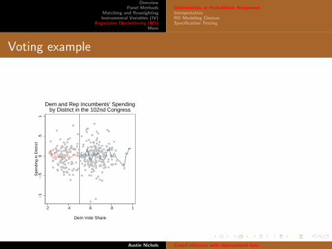
One obvious “deterministic assignment” example of a regression discontinuityoccurs in elections with two options, such as for/against (e.g. unionization) orRepublican/Democrat. Across many firms, those which unionized with apro-union vote of 80% are likely quite different along many dimensions fromthose that failed to unionize with a pro-union vote of 80%. Across manycongressional districts, those with 80% voting for Republicans are likely quitedifferent from those with 80% voting for Democrats. However, the firm thatunionizes with 50% voting for the union is probably not appreciably differentfrom the one that fails to unionize with 49.9% voting for the union. Whetheror not those people casting the few pivotal votes showed up or not is often dueto some entirely random factor (they were out sick, or their car didn’t start, orthey accidentally checked the wrong box on the ballot). DiNardo and Lee(2002) found little effect of unions using an RD design. Lee, Moretti, andButler (2004) looked at the effect of party affiliation on voting records in theUS Congress (testing the median voter theorem’s real-world utility) and Lee(2001) looked at the effect of incumbency using similar methods.






Voting example−

1−

.50

.51

S

pend

ing

in D

istr

ict

.2 .4 .6 .8 1

Dem Vote Share

Dem and Rep Incumbents’ Spendingby District in the 102nd Congress






Educational grant example

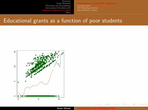
An example of “probabilistic assignment” is a US Department ofEducation grant program that is available to high-poverty school districtswithin each state. High-poverty districts are clearly different fromlow-poverty districts, but districts on either side of the cutoff point areessentially exchangeable. The first difference here is that districts thatqualify (are above the cutoff) do not automatically get the grant; theymust apply. A second difference is that low-poverty districts can enterinto consortia with high-poverty districts and get funds even though theyare below the cutoff. However, a district cannot unilaterally apply, whichcreates a discontinuity in the costs of applying at the cutoff, and we canobserve the assignment variable and the cutoff to see if there is adiscontinuity in funds received:






Educational grants as a function of poor students

05

1015

0 5 10






Local Wald Estimator

In the “sharp” or “deterministic assignment” version, the estimated treatment effect is just thejump in expected outcomes at the cutoff: in other words, the expected outcome for units justabove the cutoff (who get treated), call this y +, minus the expected outcome for units just below

the cutoff (who don’t get treated, but are supposed to be otherwise identical), call this y−, or

LATE = (y + − y−)

since the jump in the level of treatment is exactly one unit at the cutoff.

In the “fuzzy” or “probabilistic assignment” version, the jump in outcomes is “caused” by somejump in treatment that need not be one—but the ratio of coefficients method for IV, the Waldestimator, suggests how to estimate the effect of a unit change in treatment: just form the ratio ofthe jump in outcomes to the jump in treatment. The Local Wald Estimator of LATE is thus(y + − y−)/(x+ − x−), where (x+ − x−) is the estimated discontinuous jump in expectedtreatment. Note that this second estimator reduces to the first given “deterministic assignment”since (x+ − x−) = 1 in this case, so the distinction between “sharp” and “fuzzy” RD is not toosharp.






LATE

The RD estimator assumes “as-if random” assignment of the level of treatmentin the neighborhood of the cutoff, so that observations with levels of theassignment variable Z close to the cutoff Z0 form the “experimental” group.Just as is often the case with true experiments, we cannot generalize theestimated treatment effect to the rest of the population; for RD, our estimatedtreatment effect technically applies only to individuals with Z exactly equal toZ0, i.e. a set of measure zero in the population. RD is therefore a verylocalized sort of Local Average Treatment Effect (LATE) estimator with highinternal validity and low external validity.

In this respect, RD is most like a RCT, in which subjects are often selectednonrandomly from the population and then randomly assigned treatment, sothe unbiased estimate of average treatment effects applies only to the type ofsubpopulation selected into the subject pool. At least in RD, we cancharacterize exactly the population for whom we estimate the LATE: it is folkswith Z exactly equal to Z0.






Polynomial or Local Polynomial in Z

There is a great deal of art involved in the choice of some continuousfunction of the assignment variable Z for treatment and outcomes. Theresearcher chooses some high-order polynomial of Z to estimateseparately on both sides of the discontinuity, or better, a localpolynomial, local linear, or local mean smoother, where the art is in thechoice of kernel and bandwidth. Stata 10 now offers lpoly whichsupports aweights; users of prior versions can findit locpoly andexpand their data to get weighted local polynomial estimates. Thedefault in both is local mean smoothing, but local linear regression ispreferred in RD designs.






Choice of Bandwidth

There are several rule-of-thumb bandwidth choosers and cross-validationtechniques for automating bandwidth choice, but none is foolproof. McCrary(2007) contains a useful discussion of bandwidth choice, and claims that thereis no substitute for visual inspection comparing the local polynomial smootherwith the pattern in the scatterplot.

Because different bandwidth choices can produce different estimates, theresearcher should really report more than one estimate, or perhaps at leastthree: the preferred bandwidth estimate, and estimates using twice and half thepreferred bandwidth. I believe a future method might incorporate uncertaintyabout the bias-minimizing bandwidth by re-estimating many times usingdifferent bandwidth choices.

As it is, though, local polynomial regression is estimating hundreds orthousands or even hundreds of thousands of regressions. Bootstrapping theseestimates requires estimating millions of regressions, or more. Still, computingtime is cheap now.






More Choices

Of somewhat less importance, but equally art over science, is the choiceof kernel. Most researchers use the default epanechnikov kernel, but thetriangle kernel typically has better properties at boundaries, and it is theestimates at the boundaries that matter in this case.

Show the Data

Given how much choice the researcher has over parameters in asupposedly nonparametric strategy, it is always wise to show a scatteror dotplot of the data with the local polynomial smooth superimposed,so readers may be reassured no shenanigans of picking parameters wereinvolved.






Testing for Existence of a Discontinuity

The first test should be a test that the hypothesized cutoff in the assignmentvariable produces a jump in the level of treatment. In the voting example, thisis easy: the probability of winning the election jumps from zero to one at 50%,but in other settings the effect is more subtle: in the education example, thediscontinuity is far from obvious.

In any case, the test for a discontinuity in treatment X is the same as a test fora discontinuity in the outcome Y . Simply estimate a local linear regression ofX on Z , both above and below the cutoff, perhaps using a triangle kernel witha bandwidth that guarantees 10-20 observations are given positive weight atthe boundary, approaching the cutoff from either side. The local estimate atthe cutoff for regressions constrained below the cutoff is x− and the localestimate at the cutoff for regressions constrained above the cutoff is x+. Thecomputation of the difference x+ − x− can be wrapped in a program andbootstrapped for a test of discontinuity.






Testing for a Discontinuity

Assume for the sake of the example that the assignment variable Z is called share and rangesfrom 0 to 100 (e.g. percent votes received) with an assignment cutoff at 50. Then we could writea simple program:

prog discont, rclassversion 10cap drop z f0 f1g z=_n in 1/99lpoly ‘1’ share if share<50, gen(f0) at(z) nogr k(tri) bw(2) deg(1)lpoly ‘1’ share if share>=50, gen(f1) at(z) nogr k(tri) bw(2) deg(1)return scalar d=‘=f1[50]-f0[50]’endbootstrap r(d), reps(1000): discont x

The computation of the difference in outcomes y + − y− is obtained by replacing x with y above.The Local Wald Estimator of LATE is then (y + − y−)/(x+ − x−), which quantity can also becomputed in a program and bootstrapped. The SSC package rd automates many of these tasks.Imbens and Lemieux (2008) also provide analytic standard error formulae.






Testing for Sorting at the Discontinuity

McCrary (2007) gives a very detailed exposition of how one should testthis assumption by testing the continuity of the density of the assignmentvariable at the cutoff. As he points out, the continuity of the density ofthe assignment variable is neither necessary nor sufficient forexchangeability, but it is reassuring.

McCrary (2007) also provides tests of sorting around the discontinuity invoting in US Congressional elections, where there is no sorting, and inroll-call votes in Congress, where there is sorting.






Testing for Extraneous Discontinuities in Y and X

Another useful test is that there are no extra jumps in the levels oftreatment or the outcome (both should be smooth functions of theassignment variable at other points) where no hypothesized cutoff exists.This is a test of the fourth crucial assumption. One can easily pick 100random placebo cutoff points, and test the difference in X and thedifference in Y (about 5 placebo cutoffs will show significant jumps, ofcourse).






Testing for Extraneous Discontinuities in Other PotentialOutcomes

An important though supererogatory piece of evidence is that there areno jumps in variables that are not suspected to be affected by thediscontinuity. This amounts to estimating the difference h+ − h− at thecutoff for every other variable h (e.g. demographic characteristics, etc.).

This makes for some long papers, with page after page of scatterplotsshowing no relationship where none was expected, but is very reassuringthat there is not some major difference between treated and untreatedobservations around the discontinuity (i.e. these graphs are moreevidence in favor of exchangeability).





Sensitivity TestingConnections across method typesConclusionsReferences

Outline












Sensitivity Testing

The exposition by Manski (1995) demonstrates how a causal effect can be bounded under veryunrestrictive assumptions, and then the bounds can be narrowed under more restrictive parametricassumptions. Given how sensitive the QE methods are to assumptions (selection on observables,exclusion restrictions, exchangeability, etc.), some kind of sensitivity testing is order no matterwhat method is used.

Rosenbaum (2002) provides a wealth of detail on formal sensitivity testing under variousparametric assumptions. Eliason (2007) provides a short Stata example of calculating Rosenbaumbounds on treatment effects using psmatch2 and rbounds, due to DiPrete and Gangl (2004), whocompare Rosenbaum bounds in a matching model to IV estimates. sensatt by Nannicini (2006)and mhbounds by Becker and Caliendo (2007) are additional Stata programs to aid in theconstruction of bounds. Rosenbaum’s “gamma” measure of sensitivity is a useful summarymeasure of potential sensitivity, often estimated via simulation.

Lee (2005) advocates another very useful method of bounding treatment effects, used inLiebbrandt, Levinsohn, and McCrary (2005).






Panel and IV methods

Estimators such as xtivreg (see also xtivreg2 due to Schaffer 2007) orthe Arellano and Bond (1991) estimator in xtabond (see also xtabond2and Roodman 2006) offer a combination of panel methods and IVestimation.






Panel matching/reweighting

Many of the reweighting papers e.g. DiNardo, Fortin, and Lemieux(1996), Autor, Katz, and Kearney (2005), etc., are marriages ofmatching/reweighting estimators and panel methods.

The preferred estimator in Heckman, Ichimura, and Todd (1997) is amarriage of matching and diff-in-diff estimation.






Reweighted IV or RD

It is also interesting to consider reweighting so compliers in IV (thoseinduced to take a binary treatment by a single excluded binaryinstrument) look like the rest of the distribution in observable variables,or more generally to match or reweight to impute the LATE estimates tothe rest of the sample, and get an ATE estimate.

Similarly, one can imagine reweighting/matching marginal cases in RD toget at the ATE. I have not seen this in the literature, though; probablythe finite sample performance is poor.






RD meets IV

As mentioned above, the LATE estimate in the so-called “fuzzy RD”design (y+ − y−)/(x+ − x−) is a Local Wald Estimator, or a type oflocal IV.

If one were willing to dispose of local polynomials and assume a form forX and Y as functions of the assignment variable Z , the RD approach canbe recast as straight IV where the terms with Z are included instrumentsand an indicator for Z above the cutoff is the sole excluded instrument.






RD meets DDOne can also imagine estimating a diff-in-diff version of the RD estimator, given the advent ofsome policy with an eligibility cutoff, where the difference across times t and 0:[

(y +t − y−t )− (y +

0 − y−0 )]/(x+

t − x−t )

would be the estimated program impact. One would not want the difference in local Waldestimates [

(y + − y−)/(x+ − x−)]

t−

[(y + − y−)/(x+ − x−)

]0

since before the policy is implemented, one would expect (x+ − x−) to be zero, which wouldcreate instability in the estimate.

An application where this might be useful is if we expect an underlying discontinuity at the cutoffin the absence of treatment but we can use the observed jump in x and y before treatment beginsto difference that out. For example, a new treatment is applied only to those 65 or older, but thereis already an effect at 65 due to a jump in eligibility for Medicare (a large public health insurancesystem). Or a new treatment is applied only to those whose children are 18 or older, but there isalready an effect at 18 due to parents’ ideas about when children should fend for themselves. Ify +

0 − y−0 (and/or x+0 − x−0 ) is nonzero, we can give up the internal validity of regression

discontinuity, and downgrade to the internal validity of panel estimators, but get an unbiasedestimate under stronger conditions. If the jumps at the cutoff are not changing over time in theabsence of treatment, the differenced local Wald estimators will be unbiased for the local averagetreatment effect.






Conclusions

None of these methods is perfect. The gold standard, an RCT, has the bestinternal validity but may have poor external validity. Of methods usingobservational data, the RD design is closest to an RCT, and also has highinternal validity but low external validity. IV methods can eliminate bias fromselection on unobservables in the limit, but may have very poor performance infinite samples. The hypothetical internal validity of IV is high, but the practicalinternal validity of IV is often low, and the external validity not much greaterthan RD.

Panel methods can eliminate bias from selection on unobservables that do notchange over time, or satisfy other strong distributional assumptions, but therequired assumptions are often untenable in practice. Matching andreweighting methods can eliminate bias due to selection on observables, andgive efficient estimates of many types of treatment effects in many settings,but it is rarely the case that selection depends only on observables, in whichcase matching can actually exacerbate bias. Regression or matching methodsapplied to population data often have very high external validity, but internalvalidity that is often questionable.






Conclusions cont.

In practice, the data often dictate the method. If one has access toexperimental data, one worries less about selection (though IV is often used tocorrect for selection of treatment status contrary to assignment). Givenobservational data, if one can find a discontinuity in expected treatment withrespect to an observable assignment variable, one uses RD; if one can conceiveof plausible excluded instruments, one uses IV. In the absence of these featuresof the data, repeated measures may used to control for invariant unobservables,or observations may be matched on observables.

Checking that your model is not badly misspecified, and conducting variouskinds of sensitivity tests, is perhaps the most valuable way to minimize bias inpublished estimates. Nichols (2007, 2008) offers a kind of “checklist” of thingsto look at in these models (in Stata) and there will be a monograph with moreuser-friendly text and examples later this year (forthcoming from Stata Press).






Abadie, Alberto and Guido W. Imbens. 2006. “On the Failure of the Bootstrap for Matching Estimators.” NBER technical working paper325.

Abadie, Alberto, David Drukker, Jane Leber Herr, and Guido W. Imbens, 2004. “Implementing matching estimators for average treatmenteffects in Stata,” Stata Journal 4(3): 290-311

Abadie, Alberto, Joshua D. Angrist, and G. Imbens, (2002), ”Instrumental Variables Estimation of Quantile Treatment Effects,”Econometrica 70(1): 91-117.

Abadie, Alberto, and Guido W. Imbens. 2002. “Simple and Bias-Corrected Matching Estimators for Average Treatment Effects,” NBERtechnical working paper 283.

Abowd, J., Creecy, R. and Kramarz, F. 2002. “Computing person and firm effects using linked longitudinal employer-employee data.”Technical Paper 2002-06, U.S. Census Bureau.

Anderson, T. W. and H. Rubin (1949). “Estimators of the Parameters of a Single Equation in a Complete Set of Stochastic Equations.”Annals of Mathematical Statistics, 21: 570-582.

Andrews, Donald W. K.; Marcelo J. Moreira; and James H. Stock. 2007. “Performance of Conditional Wald Tests in IV Regression withWeak Instruments.” Journal of Econometrics, 139(1): 116-132. Working paper version online with supplements at Stock’s website.

Andrews, Donald W. K.; Marcelo J. Moreira; and James H. Stock. 2006. “Optimal Two-Sided Invariant Similar Tests for InstrumentalVariables Regression.” Econometrica 74: 715-752. Earlier version published as NBER Technical Working Paper No. 299 with supplementsat Stock’s website.

Andrews, Martyn, Thorsten Schank, and Richard Upward. “Practical fixed effects estimation methods for the three-way error componentsmodel.” University of Nottingham Working Paper.

Angrist, Joshua D. and Alan B. Krueger. 2000. “Empirical Strategies in Labor Economics,” in A. Ashenfelter and D. Card eds. Handbookof Labor Economics, vol. 3. New York: Elsevier Science.

Angrist, Joshua D., Guido W. Imbens and D.B. Rubin. 1996. “Identification of Causal Effects Using Instrumental Variables.” Journal ofthe American Statistical Association 91, 444-472.

Angrist, Joshua D., Guido W. Imbens, and Alan B.Krueger. 1999. “Jackknife Instrumental Variables Estimation.” Journal of AppliedEconometrics 14(1): 57-67.

Angrist, Joshua D. and Jorn-Steffen Pischke. 2009. Mostly Harmless Econometrics Princeton: Princeton University Press.


http://www.nber.org/t0325




http://post.economics.harvard.edu/faculty/moreira/papers/cwald_4.pdf

http://ksghome.harvard.edu/~JStock/ams/websupp/index.htm

http://papers.nber.org/papers/t0299

http://ksghome.harvard.edu/~JStock/ams/websupp/index.htm

http://www.nottingham.ac.uk/economics/leverhulme/staff/details/ru/leed2.pdf





Arellano, Manuel. 1987. “Computing Robust Standard Errors for Within-Groups Estimators.” Oxford Bulletin of Economics and Statistics,49: 431-34.

Arellano, M., and S. Bond. 1991. “Some tests of specification for panel data: Monte Carlo evidence and an application to employmentequations.” Review of Economic Studies 58: 277-297.

Athey, Susan and Guido W. Imbens. 2006. “Identification and Inference in Nonlinear Difference-in-Differences Models.” Econometrica 74(2): 431-497.

Autor, David H., Lawrence F. Katz, Melissa S. Kearney. 2005. “Rising Wage Inequality: The Role of Composition and Prices.” NBERWorking Paper 11628.

Baker, Michael, Dwayne Benjamin, and Shuchita Stanger. 1999. “The Highs and Lows of the Minimum Wage Effect: A Time-SeriesCross-Section Study of the Canadian Law.” Journal of Labor Economics, 17(2): 318-350.

Basmann, R.L. 1960. “On Finite Sample Distributions of Generalized Classical Linear Identifiability Test Statistics.” Journal of theAmerican Statistical Association 55(292): 650-59.

Baum, Christopher F. 2006. “Time-series filtering techniques in Stata.” Presented at NASUG5.

Baum, Christopher F., Mark E. Schaffer, Steven Stillman, and Vince Wiggins. 2006. “overid: Stata module to calculate tests ofoveridentifying restrictions after ivreg, ivreg2, ivprobit, ivtobit, reg3.” RePEc or findit overid.

Baum, Christopher F., Mark E. Schaffer, and Steven Stillman. 2007. “Enhanced routines for instrumental variables/GMM estimation andtesting.” Unpublished working paper.

Baum, Christopher F., Mark E. Schaffer, and Steven Stillman. 2003. “Instrumental variables and GMM: Estimation and testing.” StataJournal 3(1), 1-31. Also Boston College Department of Economics Working Paper No 545

Becker, Sascha O. and Andrea Ichino. 2002. “Estimation of average treatment effects based on propensity scores”, The Stata Journal2(4): 358-377. Also findit pscore for updates (e.g. Stata Journal 5(3): 470).

Becker, Sascha O. and Marco Caliendo, 2007. “mhbounds - Sensitivity Analysis for Average Treatment Effects.” IZA Discussion Paper2542.


http://www.nber.org/papers/w11628


http://links.jstor.org/sici?sici=0734-306X%28199904%2917%3A2%3C318%3ATHALOT%3E2.0.CO%3B2-B

http://www.stata.com/meeting/5nasug/TSFiltering_beamer.pdf

http://ideas.repec.org/c/boc/bocode/s396802.html

http://fmwww.bc.edu/EC-P/WP545.pdf

http://ftp.iza.org/dp2542.pdf






Blinder, Alan S. 1973. “Wage Discrimination: Reduced Form and Structural Estimates.” The Journal of Human Resources 8(4): 436-455.

Bound, John, David A. Jaeger, and Regina Baker. 1993. “The Cure Can Be Worse than the Disease: A Cautionary Tale RegardingInstrumental Variables.” NBER Technical Working Paper No. 137.

Bound, John, David A. Jaeger, and Regina Baker. 1995. “Problems with Instrumental Variables Estimation when the Correlation Betweenthe Instruments and the Endogenous Explanatory Variables is Weak.” Journal of the American Statistical Association, 90(430), 443-450.

Cameron, A. Colin, Jonah B. Gelbach, and Douglas L. Miller. 2006. “Robust Inference with Multi-Way Clustering.” NBER TechnicalWorking Paper T0327.

Cameron, A. Colin, Jonah B. Gelbach, and Douglas L. Miller. 2007. “Bootstrap-Based Improvements for Inference with Clustered Errors”FSU College of Law, Law and Economics Paper 07/002.

Chao, John C. and Norman R. Swanson. (2005). “Consistent Estimation with a Large Number of Weak Instruments.” Econometrica,73(5), 1673-1692. Working paper version available online.

Cochran, William G. 1965. “The Planning of Observational Studies of Human Populations” and discussion. Journal of the RoyalStatistical Society A128(2): 234-266.

Cochran, William G., and Donald B. Rubin. 1973. ”Controlling Bias in Observational Studies: A Review.” Sankhya 35: 417-46.

Cook, Thomas D. 2008. “Waiting for Life to Arrive: A History of the Regression-Discontinuity Design in Psychology, Statistics andEconomics.” Journal of Econometrics, 142(2).

Cragg, J.G. and S.G. Donald. (1993). “Testing Identifiability and Specification in Instrumental Variable Models,” Econometric Theory, 9,222-240.

Dahl, Gordon and Lance Lochner. 2005. “The Impact of Family Income on Child Achievement.” NBER Working Paper 11279.

Devereux, Paul J. 2007. “Improved Errors-in-Variables Estimators for Grouped Data.” Journal of Business and Economic Statistics, 25(3):278-287.


http://links.jstor.org/sici?sici=0022-166X%28197323%298%3A4%3C436%3AWDRFAS%3E2.0.CO%3B2-U

http://papers.nber.org/papers/t0137

http://links.jstor.org/sici?sici=0162-1459%28199506%2990%3A430%3C443%3APWIVEW%3E2.0.CO%3B2-U

http://nber.org/t0327

http://nber.org/t0327

http://ssrn.com/abstract=956890

http://papers.ssrn.com/sol3/papers.cfm?abstract_id=410809

http://links.jstor.org/sici?sici=0035-9238%281965%29128%3A2%3C234%3ATPOOSO%3E2.0.CO%3B2-F

http://links.jstor.org/sici?sici=0035-9238%281965%29128%3A2%3C234%3ATPOOSO%3E2.0.CO%3B2-F

http://nber.org/papers/W11279





DiNardo, John. 2002. “Propensity Score Reweighting and Changes in Wage Distributions” University of Michigan Working Paper.

DiNardo, John and David Lee. 2002. “The Impact of Unionization on Establishment Closure: A Regression Discontinuity Analysis ofRepresentation Elections.” NBER Working Paper 8993.

DiNardo, John, Nicole M. Fortin, and Thomas Lemieux. 1996. “Labor Market Institutions and the Distribution of Wages, 1973-1992: ASemiparametric Approach.” Econometrica, 64(5): 1001-1044.

DiNardo, John and Justin L. Tobias. 2001. “Nonparametric Density and Regression Estimation.” The Journal of Economic Perspectives,15(4): 11-28.

DiPrete, Thomas A. and Markus Gangl. 2004. “Assessing Bias in the Estimation of Causal Effects: Rosenbaum Bounds on MatchingEstimators and Instrumental Variables Estimation with Imperfect Instruments.” Sociological Methodology, 34: 271-310. Stata code toestimate Rosenbaum bounds

Dufour, Jean-Marie. 2003. “Identification, Weak Instruments, and Statistical Inference in Econometrics.” Canadian Journal of Economics,36, 767-808.

Dufour, Jean-Marie and Mohamed Taamouti. 1999; revised 2003. “Projection-Based Statistical Inference in Linear Structural Models withPossibly Weak Instruments.” Manuscript, Department of Economics, University of Montreal.

Dufour, Jean-Marie and Mohamed Taamouti. 2007. “Further results on projection-based inference in IV regressions with weak, collinear ormissing instruments.” Journal of Econometrics, 139(1): 133-153.

Eliason, Scott R. 2007. “Calculating Rosenbaum Bounds in Stata: Average Causal Effects of College v. HS Degrees on Wages Example.”University of Minnesota paper. See also this website.

Fisher, Ronald A. 1918. “The causes of human variability.” Eugenics Review 10: 213-220.

Fisher, Ronald A. 1925. Statistical Methods for Research Workers. Edinburgh: Oliver and Boyd.

Fisher, Ronald A. 1926. “The arrangement of field experiments.” Journal of the Ministry of Agriculture of Great Britain, 33:503–513.

Frolich, Markus. 2007a. “Nonparametric IV Estimation of Local Average Treatment Effects with Covariates.” Journal of Econometrics139 (1), 35-75. Also IZA Discussion Paper 588.


http://www-personal.umich.edu/~jdinardo/bztalk5.pdf

http://nber.org/papers/w8993

http://links.jstor.org/sici?sici=0012-9682%28199609%2964%3A5%3C1001%3ALMIATD%3E2.0.CO%3B2-K

http://links.jstor.org/sici?sici=0895-3309%28200123%2915%3A4%3C11%3ANDARE%3E2.0.CO%3B2-4

http://links.jstor.org/sici?sici=0895-3309%28200123%2915%3A4%3C11%3ANDARE%3E2.0.CO%3B2-4

http://www.wzb.eu/ars/ab/pdf/gangl_rbounds.zip

http://www.wzb.eu/ars/ab/pdf/gangl_rbounds.zip

http://www.fas.umontreal.ca/SCECO/dufour/Dufour_Taamouti_1999_Projections_W.pdf

http://www.soc.umn.edu/~eliason/index_files/RB_Example.pdf

http://www.soc.umn.edu/~eliason/index_files/AdvTopics_CausalInference.htm






Frolich, Markus. 2007b. “Propensity score matching without conditional independence assumptionwith an application to the gender wagegap in the United Kingdom.” The Econometrics Journal 10(2), 359407.

Frolich, Markus. 2004. “What is the Value of Knowing the Propensity Score for Estimating Average Treatment Effects?” EconometricReviews 23(2): 167-174. Also IZA Discussion Paper 548.

Goldberger, Arthur S. 1972. “Selection bias in evaluating treatment effects: Some formal illustrations.” Discussion paper 123-72, Institutefor Research on Poverty, University of Wisconsin, Madison.

Goldberger, Arthur S., and 0tis D. Duncan. 1973. Structural Equation Models in the Social Sciences. New York: Seminar Press.

Gomulka, Joanna, and Nicholas Stern. 1990. “The Employment of Married Women in the United Kingdom 1970-83.” Economica 57:171-199.

Hahn, Jinyong, Petra Todd, and Wilbert Van der Klaauw. 2001. “Identification and Estimation of Treatment Effects with aRegression-Discontinuity Design.” Econometrica 69(1): 201-209.

Hardin, James W., Henrik Schmiediche, and Raymond J. Carroll. 2003. “Instrumental variables, bootstrapping, and generalized linearmodels.” Stata Journal 3(4): 351-360. See also http://www.stata.com/merror/.

Heckman, James J. and Edward Vytlacil. 1999. “Local Instrumental Variables and Latent Variable Models for Identifying and BoundingTreatment Effects.” Proceedings of the National Academy of Sciences of the United States of America 96:4730-34.

Heckman, James J. and Edward Vytlacil. 2000. “The Relationship between Treatment Parameters within a Latent Variable Framework.”Economics Letters 66:33-39.

Heckman, James J. and Edward Vytlacil. 2004. “Structural Equations, Treatment Effects and Econometric Policy Evaluation.”Econometrica 73(3): 669738.

Heckman, James J., Hidehiko Ichimura, and Petra E. Todd. 1997. “Matching as an Econometric Evaluation Estimator: Evidence fromEvaluating a Job Training Programme.” Review of Economic Studies 64(4): 605-654.

Hirano, Keisuke, Guido W. Imbens, and Geert Ridder, 2003. “Efficient Estimation of Average Treatment Effects Using the EstimatedPropensity Score.” Econometrica 71(4): 1161-1189. (See also NBER WP T0251.



http://www.stata.com/merror/

http://links.jstor.org/sici?sici=0034-6527%28199710%2964%3A4%3C605%3AMAAEEE%3E2.0.CO%3B2-I

http://www.nber.org/papers/t0251.pdf





Holland, Paul W. 1986. “Statistics and causal inference.” Journal of the American Statistical Association 8(396): 945-960.

Imbens, Guido and Jeffrey Wooldridge. “What’s New in Econometrics.” NBER Summer Institute Course notes.

Imbens, Guido and Thomas Lemieux. 2008. “Regression Discontinuity Designs: A Guide to Practice.” Journal of Econometrics, 142(2).See also NBER Working Paper 13039.

Imbens, Guido W. 2004. “Nonparametric Estimation of Average Treatment Effects Under Exogeneity: A Review.” Review of Economicsand Statistics 86(1): 4-29, 06. Earlier version available as NBER Technical Working Paper 0294.

Imbens, Guido W. 2006. “Matching methods for estimating treatment effects using Stata.” Presented at NASUG6.

Imbens, Guido W. and Joshua D. Angrist. 1994. “Identification and Estimation of Local Average Treatment Effects.” Econometrica62(2): 467-75

Juhn, Chinhui, Kevin M. Murphy, Brooks Pierce. 1993. “Wage Inequality and the Rise in Returns to Skill.” Journal of Political Economy101(3): 410-442.

Juhn, Chinhui, Kevin M. Murphy, Brooks Pierce. 1991. “Accounting for the Slowdown in Black-White Wage Convergence.” in Workersand Their Wages, ed. Marvin Kosters, Washington, DC: AEI Press.

Kaushal, Neeraj. 2007. “Do Food Stamps Cause Obesity? Evidence from Immigrant Experience.” NBER Working Paper No. 12849

Kezdi, Gabor. 2004. “Robust Standard Error Estimation in Fixed-Effects Panel Models.” Hungarian Statistical Review Special(9): 96-116.

Kinal, Terrence W. 1980. “The Existence of Moments of k-Class Estimators.” Econometrica, 48(1), 241-250.

Kleibergen, Frank. 2002. “Pivotal Statistics for Testing Structural Parameters in Instrumental Variables Regression.” Econometrica,70(5), 1781-1803.


http://links.jstor.org/sici?sici=0162-1459%28198612%2981%3A396%3C945%3ASACI%3E2.0.CO%3B2-7

http://www.nber.org/~confer/2007/si2007/wneprg.html


http://www.nber.org/papers/t0294

http://www.stata.com/meeting/5nasug/Imbens_stata_06july.pdf

http://papers.nber.org/papers/w12849

http://portal.ksh.hu/pls/portal/docs/PAGE/STATSZEMLE/STATSZEMLE_ARCHIVUM/2004_ARCHIVUM/2004_SPECIAL_S9_ARCHIVUM/KEZDI.PDF

http://links.jstor.org/sici?sici=0012-9682%28198001%2948%3A1%3C241%3ATEOMOK%3E2.0.CO%3B2-D

http://links.jstor.org/sici?sici=0012-9682%28200209%2970%3A5%3C1781%3APSFTSP%3E2.0.CO%3B2-0

http://links.jstor.org/sici?sici=0012-9682%28200209%2970%3A5%3C1781%3APSFTSP%3E2.0.CO%3B2-0





Kleibergen, Frank. 2007. “Generalizing weak instrument robust IV statistics towards multiple parameters, unrestricted covariance matricesand identification statistics.” Journal of Econometrics 139(1): 181-216.

Kleibergen, Frank and Richard Paap. 2006. “Generalized reduced rank tests using the singular value decomposition.” Journal ofEconometrics 133(1): 97-126. Preprint.

Lee, David S., Enrico Moretti, and Matthew J. Butler. 2004. “Do Voters Affect Or Elect Policies? Evidence From The U. S. House.”Quarterly Journal of Economics 119(3): 807-859.

Lee, David S. 2001. “The Electoral Advantage to Incumbency and Voters’ Valuation of Politicians’ Experience: A RegressionDiscontinuity Analysis of Elections to the U.S. House.” NBER Working Paper 8441. New version “Randomized Experiments fromNon-random Selection in U.S. House Elections” forthcoming in Journal of Econometrics with a Supplemental Mathematical Appendix.

Lee, David S. 2005. “Training, Wages, and Sample Selection: Estimating Sharp Bounds on Treatment Effects.” NBER Working Paper11721 with errata. Previous version: Trimming for Bounds on Treatment Effects with Missing Outcomes, NBER Technical Working Paper277.

Lee, David S. and David Card. 2008. “Regression Discontinuity Inference with Specification Error.” Journal of Econometrics, 142(2). Seealso NBER Technical Working Paper 322 and previous version: Center for Labor Economics Working Paper 74.

Lee, Lung-Fei. 1992. “Amemiya’s Generalized Least Squares and Tests of Overidentification in Simultaneous Equation Models withQualitative or Limited Dependent Variables.” Econometric Reviews 11(3): 319-328.

Leibbrandt, Murray, James Levinsohn, and Justin McCrary. 2005. “Incomes in South Africa Since the Fall of Apartheid.” NBER WorkingPaper 11384.

Leuven, Edwin and Barbara Sianesi. 2003. “psmatch2: Stata module to perform full Mahalanobis and propensity score matching,common support graphing, and covariate imbalance testing.” RePEc or findit psmatch2.

Machado, Jos and Jos Mata. 2005. “Counterfactual Decompositions of Changes in Wage Distributions Using Quantile Regression.”Journal of Applied Econometrics 20(4): 445-65.

Manski, Charles F. 1995. Identification Problems in the Social Sciences. Cambridge, MA: Harvard University Press.

McCrary, Justin. 2007. “Manipulation of the Running Variable in the Regression Discontinuity Design: A Density Test.” NBER TechnicalWorking Paper 334.


http://www.econ.brown.edu/fac/Frank_Kleibergen/revrank1.pdf


http://www.princeton.edu/~davidlee/wp/AppendixC.pdf



http://www.princeton.edu/~davidlee/wp/typo_trim.pdf

http://www.nber.org/papers/T0322



http://ideas.repec.org/c/boc/bocode/s432001.html

http://nber.org/papers/t0334

http://nber.org/papers/t0334





Mikusheva, Anna. 2005. “Robust Confidence Sets in the Presence of Weak Instruments.” Unpublished manuscript, Harvard University.

Mikusheva, Anna and Brian P. Poi. 2006. “Tests and confidence sets with correct size in the simultaneous equations model withpotentially weak instruments.” The Stata Journal 6(3): 335-347. Working paper.

Moreira, Marcelo J. 2001. “Tests With Correct Size When Instruments Can Be Arbitrarily Weak.” Working paper available online.

Moreira, Marcelo J. 2003. “A Conditional Likelihood Ratio Test for Structural Models.” Econometrica, 71 (4), 1027-1048. Working paperversion available on Moreira’s website.

Morgan, Stephen L. and David J. Harding. 2006. “Matching Estimators of Causal Effects: Prospects and Pitfalls in Theory and Practice.”Sociological Methods and Research 35(1)3-60.

Nannicini, Tommaso. 2006. “A simulation-based sensitivity analysis for matching estimators.” presented at NASUG5, working paperonline.

Newey, W.K. 1987. “Efficient Estimation of Limited Dependent Variable Models with Endogeneous Explanatory Variables”. Journal ofEconometrics 36: 231-250.

Neyman, Jerzy. 1923. “On the Application of Probability Theory to Agricultural Experiments: Essay on Principles, Section 9,” translatedwith an introduction by D. M. Dabrowska and T. P. Speed. 1990. Statistical Science 5(4): 465-472.

Neyman, Jerzy, K. Iwaskiewicz, and St. Kolodziejczyk. 1935. “Statistical problems in agricultural experimentation” (with discussion).Supplement to the Journal of the Royal Statistical Society 2(2): 107-180.

Nichols, Austin. 2006. “Weak Instruments: An Overview and New Techniques.” presented at NASUG5.

Nichols, Austin. 2007. “Causal inference with observational data.” Stata Journal 7(4): 507-541.

Nichols, Austin. 2008. “Erratum and discussion of propensity score reweighting.” Stata Journal 8(4): 532-539.

Oaxaca, Ronald. 1973. “Male-Female Wage Differentials in Urban Labor Markets.” International Economic Review 14(3): 693-709.

Orr, Larry L., Howard S. Bloom, Stephen H. Bell, Fred Doolittle, Winston Lin, and George Cave. 1996. Does training for thedisadvantaged work? Evidence from the national JTPA Study. Washington, DC: The Urban Institute Press.


http://www.stata-press.com/journals/sjabstracts/st0033_2.pdf

http://www.people.fas.harvard.edu/~mikouch/paper-2/tests_and_confsets.pdf

http://emlab.berkeley.edu/users/cle/wp/wp37.pdf

http://post.economics.harvard.edu/faculty/moreira/papers/LR.pdf

http://post.economics.harvard.edu/faculty/moreira/papers/LR.pdf

http://repec.org/nasug2006/pres_Stata_1.pdf

http://repec.org/nasug2006/sensatt_wp.pdf

http://repec.org/nasug2006/sensatt_wp.pdf

http://links.jstor.org/sici?sici=0883-4237%28199011%295%3A4%3C465%3AOTAOPT%3E2.0.CO%3B2-M

http://links.jstor.org/sici?sici=1466-6162%281935%292%3A2%3C107%3ASPIAE%3E2.0.CO%3B2-K

http://www.stata.com/meeting/5nasug/wiv.pdf

http://www.stata-journal.com/article.html?article=st0136

http://www.stata-journal.com/article.html?article=st0136_1

http://links.jstor.org/sici?sici=0020-6598%28197310%2914%3A3%3C693%3AMWDIUL





Pearl, Judea. 2000. Causality: Models, Reasoning, and Inference. Cambridge: Cambridge University Press.

Poi, Brian P. 2006. “Jackknife instrumental variables estimation in Stata.” Stata Journal 6(3): 364-376.

Rabe-Hesketh, Sophia, Anders Skrondal, and Andrew Pickles. 2002. “Reliable estimation of generalised linear mixed models usingadaptive quadrature.” Stata Journal 2: 1-21. See also [http://gllamm.org].

Roodman, David M. 2006. “How to Do xtabond2: An Introduction to Difference and System GMM in Stata.” CGDev WP 103 andpresentation at NASUG5.

Rosenbaum, Paul R. 2002. Observational Studies. New York: Springer.

Rosenbaum, Paul R. and Donald B. Rubin. 1983. “The Central Role of the Propensity Score in Observational Studies for Causal Effects.”Biometrika 70(1): 41-55.

Rubin, Donald B. 1974. “Estimating Causal Effects of Treatments in Randomized and Nonrandomized Studies.” Journal of EducationalPsychology 66: 688-701.

Sargan, J.D. 1958. “The Estimation of Economic Relationships Using Instrumental Variables.” Econometrica 26: 393-415.

Schaffer, Mark E., and Stillman, Steven. 2006. “xtoverid: Stata module to calculate tests of overidentifying restrictions after xtivreg,xtivreg2, xthtaylor.” http://ideas.repec.org/c/boc/bocode/s456779.html

Schaffer, Mark E. 2007. “xtivreg2: Stata module to perform extended IV/2SLS, GMM and AC/HAC, LIML and k-class regression forpanel data models.” http://ideas.repec.org/c/boc/bocode/s456501.html

Schechtman, Edna and Shlomo Yitzhaki. 2001. “The Gini Instrumental Variable, or ’The Double IV Estimator’.” at SSRN.

Smith, Jeffrey A., and Petra E. Todd. 2005. “Does Matching Overcome Lalonde’s Critique of Nonexperimental Estimators?” Journal ofEconometrics 125: 305-353.


http://gllamm.org

http://repec.org/nasug2006/howtodoxtabond2.cgdev.pdf

http://repec.org/nasug2006/How2Do_xtabond2.ppt

http://links.jstor.org/sici?sici=0006-3444%28198304%2970%3A1%3C41%3ATCROTP%3E2.0.CO%3B2-Q

http://ssrn.com/abstract=281091





Smith, Jeffrey A., and Petra E. Todd. 2001. “Reconciling Conflicting Evidence on the Performance of Propensity-Score MatchingMethods.” The American Economic Review 91(2): 112-118.

Song, Kyungchul. 2009. “Efficient Estimation of Average Treatment Effects under Treatment-Based Sampling.” PIER Working Paper09-011.

Staiger, Douglas and James H. Stock (1997). “Instrumental Variables Regression with Weak Instruments.” Econometrica, 65, 557-586.

Stock, James H. and Motohiro Yogo (2005), “Testing for Weak Instruments in Linear IV Regression.” Ch. 5 in J.H. Stock and D.W.K.Andrews (eds), Identification and Inference for Econometric Models: Essays in Honor of Thomas J. Rothenberg, Cambridge UniversityPress. Originally published 2001 as NBER Technical Working Paper No. 284; newer version (2004) available at Stock’s website.

Stock, James H.; Jonathan H. Wright; and Motohiro Yogo. (2002). “A Survey of Weak Instruments and Weak Identification inGeneralized Method of Moments.” Journal of Business and Economic Statistics, 20, 518-529. Available from Yogo’s website.

Stock, James H. and Mark W. Watson. 2006. “Heteroskedasticity-Robust Standard Errors for Fixed Effects Panel Data Regression.”NBER Technical Working Paper 323.

Thistlewaite, D. L., and Campbell, Donald T. (1960). “Regression-Discontinuity Analysis: An Alternative to the Ex-Post FactoExperiment.” Journal of Educational Psychology 51: 309-317.

Tukey, J. W. 1954. “Causation, regression and path analysis,” in Statistics and Mathematics in Biology. Ames: Iowa State College Press.

Wold, Herman. 1956. “Causal inference from observational data: A review of ends and means.” Journal of the Royal Statistical Society.A119(1): 28-61.

Wooldridge, J.M. 2002. Econometric Analysis of Cross Section and Panel Data. Cambridge, MA: MIT Press. Available from Stata.com.

Yun, Myeong-Su. 2004. “Decomposing Differences in the First Moment.” Economics Letters 82(2): 275-280. See also IZA DiscussionPaper 877.

Yun, Myeong-Su. 2005a. “A Simple Solution to the Identification Problem in Detailed Wage Decompositions.” Economic Inquiry 43(4):766-772. See also IZA Discussion Paper 836.

Yun, Myeong-Su. 2005b. “Normalized Equation and Decomposition Analysis: Computation and Inference.” IZA Discussion Paper 1822.


http://links.jstor.org/sici?sici=0002-8282%28200105%2991%3A2%3C112%3ARCEOTP%3E2.0.CO%3B2-W

http://pier.econ.upenn.edu/Archive/09-011.pdf

http://pier.econ.upenn.edu/Archive/09-011.pdf

http://links.jstor.org/sici?sici=0012-9682%28199705%2965%3A3%3C557%3AIVRWWI%3E2.0.CO%3B2-Z

http://papers.nber.org/papers/t0284.pdf

http://ksghome.harvard.edu/~JStock/ams/websupp/rfa_7.pdf

http://finance.wharton.upenn.edu/~yogo/papers/published/JBES1002.pdf

http://www.nber.org/papers/T0323

http://links.jstor.org/sici?sici=0035-9238%281956%29119%3A1%3C28%3ACIFODA%3E2.0.CO%3B2-%23

http://links.jstor.org/sici?sici=0035-9238%281956%29119%3A1%3C28%3ACIFODA%3E2.0.CO%3B2-%23

http://stata.com/bookstore/cspd.html




http://www.iza.org/en/webcontent/publications/papers/viewAbstract?dp_id=1822

causal inference with observational data - boston collegefm · causal inference with observational...

Documents