Causal GMs10708, Fall 2020

Pradeep Ravikumar

1 Introduction

So far we have studied PGMs which are statistical models. Given such a statistical model, onecould use probabilistic reasoning to deduce likely observations and outcomes. And conversely,given a set of observations and outcomes, one could then use statistical learning to infer thelikely underlying statistical model. But in the real world, we do not just have passivelyobserved data, but also outcomes of active interventions. The counterpart of statisticalmodels here is a causal model. We could use causal reasoning to infer the likely outcomes ofinterventions and changes to the environment, and conversely, use causal learning to learnsuch causal models given data comprising passive observations as well as actively intervenedoutcomes.

Thus, a causal model could be viewed as subsuming a statistical model, just as the corre-sponding set of outcomes, both passive and active, subsumes the set of passively observedoutcomes.

But what is the connection between a causal model and a statistical model? The followingimportant principle could be viewed as providing one such link.

Definition 1 (Reichenbach’s Common Cause Principle) If two random variables Xand Y are statistically dependent, then there exists a third random variable Z that is acommon cause (possibly coinciding with either X or Y ), such that X ⊥⊥ Y |Z.

Remark: Spurious Dependences. Note that in some cases where we only observe therandom variables via a finite set of samples from their corresponding distributions, it ispossible for there to be a spurious observed dependence: the principle above then doesnot apply. When we do not have iid data, and instead see samples from two time-varyingstochastic processes, then it might seem that the two variables are dependent. This is forinstance what leads people to claim analogues of the increasing number of Shrek moviesbeing associated with global warming. In such a case, we could view time itself as a commoncause. In certain cases, the samples we observe of X and Y are implicitly conditioned ona specific value of some other variable Z. When this conditioning variable is a downstream“effect” of X and Y , then we know that this results in observed conditional dependence ofX and Y : this is also called selection bias. In this case again the Reichenbach’s principledoes not apply, since we do not observe marginal dependence of X and Y .

1

Time and Causality. In certain accounts, causality is intrinsically associated with timein the sense that the effect variable is observed after the cause variable. However, it isnot necessary we incorporate time in our causal modeling machinery. It could be that theobservations cannot be mapped to specific time, or might even be equilibrium observations.For instance, consider motivation as cause, and grades as the effect: the former cannot bemapped to a specfic time instance. Mapping to time is most common in hard sciences suchas physics and chemistry.

1.1 Hierarchy of Models

We thus have the following hierarchy of mathematical models for reasoning in complex en-vironments. A statistical model can answer observational queries, but not interventional, orcounterfactual queries.A causal graphical model can answer both observational and interventional queries, but notcounterfactual ones.A structural causal model can answer observational, interventional, as well as counterfactualqueries.Mechanistic or Physical Models can not only all of above queries, but moreover have com-ponents that can be mapped to the real world, so that they additionally provide “scien-tific/physical insight”.

1.2 Interventions

The key distinction between statistical and causal setting arises from outcomes of interven-tions. An intervention comprises simply of setting a variable to a particular value. We oftenassume this is an ideal intervention: where we set the value of a specific variable without“setting” values of other variables immediately. There could still be causal effects conse-quently, which we are actually interested in measuring. Interventions might not be possibleper se. For instance, we cannot simply instantaneously intervene on age of a person.

As we will see counterfactuals are a slightly more subtle notion: here, we do observe thevalue of the specific variable, but want to reason about the outcome if we set the variableto some other value. This results in some slightly different conclusions, as we will see in thesequel.

2

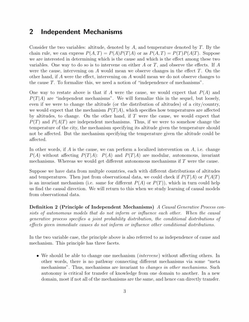
2 Independent Mechanisms

Consider the two variables: altitude, denoted by A, and temperature denoted by T . By thechain rule, we can express P (A, T ) = P (A)P (T |A) or as P (A, T ) = P (T )P (A|T ). Supposewe are interested in determining which is the cause and which is the effect among these twovariables. One way to do so is to intervene on either A or T , and observe the effects. If Awere the cause, intervening on A would mean we observe changes in the effect T . On theother hand, if A were the effect, intervening on A would mean we do not observe changes tothe cause T . To formalize this, we need a notion of “independence of mechanisms”.

One way to restate above is that if A were the cause, we would expect that P (A) andP (T |A) are “independent mechanisms”. We will formalize this in the sequel, but loosely,even if we were to change the altitude (or the distribution of altitudes) of a city/country,we would expect that the mechanism P (T |A), which specifies how temperatures are affectedby altitudes, to change. On the other hand, if T were the cause, we would expect thatP (T ) and P (A|T ) are independent mechanisms. Thus, if we were to somehow change thetemperature of the city, the mechanism specifying its altitude given the temperature shouldnot be affected. But the mechanism specifying the temperature given the altitude could beaffected.

In other words, if A is the cause, we can perform a localized intervention on A, i.e. changeP (A) without affecting P (T |A): P (A) and P (T |A) are modular, autonomous, invariantmechanisms. Whereas we would get different autonomous mechanisms if T were the cause.

Suppose we have data from multple countries, each with different distributions of altitudesand temperatures. Then just from observational data, we could check if P (T |A) or P (A|T )is an invariant mechanism (i.e. same for different P (A) or P (T )), which in turn could helpus find the causal direction. We will return to this when we study learning of causal modelsfrom observational data.

Definition 2 (Principle of Independent Mechanisms) A Causal Generative Process con-sists of autonomous models that do not inform or influence each other. When the causalgenerative process specifies a joint probability distribution, the conditional distributions ofeffects given immediate causes do not inform or influence other conditional distributions.

In the two variable case, the principle above is also referred to as independence of cause andmechanism. This principle has three facets.

• We should be able to change one mechanism (intervene) without affecting others. Inother words, there is no pathway connecting different mechanisms via some “metamechanisms”. Thus, mechanisms are invariant to changes in other mechanisms. Suchautonomy is critical for transfer of knowledge from one domain to another. In a newdomain, most if not all of the mechanisms are the same, and hence can directly transfer.

3

• Each mechanism should not provide “information” about other mechanisms. One as-pects of this is with respect to changes: change in one mechanism should not provideinformation on how other mechanisms have changed. But there should be no informa-tion flow even in the absence of changes.

• Suppose the conditional distributions can be specified deterministically given the set ofobserved random variables, and additional noise variables. In the two variable, cause-effect model, case, suppose that C,E are two variables, with conditional distributionsspecified as:

C = NC

E = fE(C,NE),

where NC , NE are additional noise variables, and fE is a deterministic function. ThenNC , NE are statistically independent.

It can be seen that such statistical independence is necessary for independence ofmechanisms.

To see this, note that the noise variable N acts as a gate, whose value specifies oneof many deterministic mechanisms, which we can rewrite as E = fN(C). So if N isdependent on some other noise variable M for some other mechanism say E ′ = gM(C),then there is information leakage between different mechanisms.

The third facet is something we have a good understanding of, namely statistical indepen-dence of noise variables. But how do we formalize the first two facets which need some wayof specifying independence of mechanisms (rather than random variables). We will see thatin the sequel.

3 Cause Effect Models

It is instructive to first study causal models in the simplest possible setting with just twovariables: a cause variable C and an effect variable E. This would allow us to isolate theadditional facets of a causal model beyond that of a statistical model.

A common approach of specifying a causal model is via a so-called Structural Causal Model(SCM):

C = NC

E = fE(C,NE),

where NC , NE are independent noise variables, and fE is a deterministic function. This isassociated with a “causal graph” with nodes C,E and a directed edge C → E.

4

3.1 Interventions

When we intervene on a variable, say E, we simply substitute its existing causal mechanism(E = fE(C,NE)),for a substitute intervened one.

The simplest such intervention is where the substitute mechanism is simply setting E toa constant. This is referred to as a hard intervention, and we will denote the resultingcausal model as P (E=e). This is to be contrasted with the more general soft interventions,where the substitute mechanism could be a more general e.g. E = g(C, NE). We will denote

the resulting intervened causal model via P (E=g(C,NE)).

If the causal graph is C → E, when we intervene on the effect variable, we do not expectthe cause mechanism to change. Accordingly,

P(E=e)C = PC 6= PC|E=e.

This clearly shows that intervening is not the same as conditioning. But on the other handwhen we intervene on the cause variable:

P(C=c)E = PE|C=c 6= PE.

Moreover, in the effect-intervened causal model P(E=NE)C,E , we have that C ⊥⊥ E, but which

does not hold in the cause-intervened causal model: P(C=NC)C,E .

3.2 Counterfactuals

Suppose we have a disease that could result in blindness, and a candidate treatment for thisdisease. Let T denote the binary variable on whether or not to administer the treatmentand let B denote the binary variable on whether or not the disease causes blindness. Nowsuppose that for 99% of patients, the treatment leads to a cure, and if not treated, theyget blind. While for the remaining 1% of patients, the treatment leads to blindness, and ifnot treated, they get cured. So any patient belongs to one of these two categories, which inturn depends on a condition NB ∈ 0, 1 which is unknown to the doctor. We thus have thefollowing causal model:

T = NT

B = T NB + (1− T )(1−NB),

where NB ∼ Ber(0.01).

5

Suppose somebody gets the treatment, but are blinded. A natural question would then be:what would have happened if we had not given that person the treatment?

This is a counterfactual question. Note that unlike the intervention case, here we do observethe values of the variables: T = 1, B = 1. Plugging these into the SCM above, we get thatNT = 1, NB = 1. Suppose we plug these values of the noise variables back into the SCM:this then yields the counterfactual SCM:

T = 1

B = T + (1− T )0 = T.

Let us denote this counterfactual SCM by C ′. The counterfactual question asked above isthen reasoning with an intervention on this counterfactual SCM: C ′(T=0). This can be seento be the SCM: is then the SCM:

T = 0

B = T,

which places all mass on (0, 0). So the answer to the counterfactual query is that the patientwould have been cured if not treated!

Does that mean the doctor commited malpractice? Note however that the condition (affect-ing the noise variable NB) is unknown apriori. All the doctor could thus use apriori are theinterventional probabilities :

P (T=1)(B = 0) = P (NB = 0) = 0.99

P (T=0)(B = 0) = P (NB = 1) = 0.01,

which does warrant the doctor treating the patient.

So for answering counterfactual questions, we first set up a counterfactual SCM by inferringnoise variables given the observed values of the observed variables, and then use interventionbased causal reasoning with this SCM. A consequence of this is that two SCMs with thesame interventional probabilities can lead to different counterfactual probabilities.

Consider the following SCM:

C = NC

E = nE(C),

where without loss of generality we have combined the functional and noise elements ofthe effect mechanism in the earlier SCM into a random function nE . Suppose C takes

6

values in the finite set C = [k], and E in some other finite set E. Then any deterministicfunction g from C to E can be associated with the vector (g(1), . . . , g(k)) ∈ Ek. Thus theset of random functions g is associated with a random vector (g(1), . . . , g(k)). Since C is

the cause, and E is the effect, P(C=j)E = PE|C=j = Pg(j), so that the observational and

interventional distributions (when we intervene on the cause) coincide, and moreover onlydepend on the marginal distributions Pg(j) of the random noise function g.

But on observing some values (c, e) of the cause and effect variables, the counterfactual SCMis then given by:

C = c

E = nE(C) | (nE(c) = e).

Thus the counterfactual SCM explicitly depends on the joint distribution of nE, and ac-cordingly counterfactual queries such as “if c had been different, then would e be different?”necessarily involve reasoning with the joint distribution of nE. For instance, suppose weobserve (j, e), and suppose as before we identify nE with a random vector (g(1), . . . , g(k)).Then, in the counterfactual SCM above:

C = j

E ∼ g | g(j) = e

The counterfactual query of what would have happened were C = j′ instead, could be

answered by P(C=j′)E = PE|C=j′ = Pg(j′)|g(j)=e, which explicitly involves the joint distribution

of the noise distribution g.

4 Causality: Connections to Unsupervised Learning

In the Unsupervised Learning task of clustering, we are given (samples based access to) thedistribution PX of some variables X, and are asked to infer PY |X of some “cluster” label Y .Note that we do not have any access, sampling based or otherwise, to PY or PX,Y .

Suppose X is the cause, and Y is the effect. Then by independence of causal mechanisms,PX has no information about PY |X . So unsupervised learning “in a causal direction” is notpossible.

On the other hand, suppose X is the effect, and Y is the cause. then PX may have infoabout PY |X . As an example, suppose Y ∈ −1, 1, and X = Y µ+NX where NX ∼ N (0, 1),then, PX is a Gaussian mixture model, from which can recover the Gaussian componentsPX|Y and hence via Bayes rule PY |X .

7

Remark. Note that if we aim to obtain an optimal decision function f ∗inF , and optimizeout PY |X over a set P , wrt some optimality criterion, then this optimal f ∗ by definition willdepend on PX .

As an example, suppose we use a Bayesian optimality criertion, with respect to some priorπ over distributions PY |X . Then solving for:

arg inffinF

EPY |X πloss(f, PY |X , PX),

clearly only depends on PX .

This is also the case with a minimax optimality criterion:

arg inffinF

supPY |X inP

loss(f, PY |X , PX),

clearly only depends on PX .

Thus the key point is not whether the decision function of interest depends only on PX , butrather is an informational statement about PX itself: whether PY |X is idenfitiable given PX .

5 Causality: Connections to Domain Adaptation

Suppose X is the cause, and Y the effect. Then even if we change PX (covariate shift),the “autonomous mechanism” PY |X need not change, and hence could be used even in thecovariate shifted domain. Of course, it is still possible that PY |X also changes (independentof the changes in PX), but by the independence principle, the new P ′X has no info aboutP ′Y |X so we might as well use the old PY |X in the absence of further information.

The above is only justified in the causal direction. Whereas, in the anti-causal direction, anychange in PX could also entail changes in PY |X , and indeed we could even aim to estimatethis change. In one extreme, P ′X could make P ′Y |X identifiable, so we could use unsupervisedlearning to infer this.

Causality seems to have a lot to say about domain adaptation and transfer problems, butmuch is still open.

6 General Structural Causal Models (SCMs)

An SCM C consists of a DAG G, and a collection of “structural assignments”:

Xj = fj(PAj, Nj),

8

where PAj are parents of Xj in G, and (N1, ..., Np) are independent noise terms. Eachsuch assignment is simply an alternative characterization of the conditional distribution ofXj given PAj. The variables PAj are called direct causes of Xj, and Xj is a direct effectof its causes. SCMs are also called Structural Equation Models (SEMs). When fj(·) arenon-linear, these are called non-linear SCMs/SEMs.

Proposition 3 An SCM entails a unique joint distribution over (X1, ..., Xp).

This just follows from how in the case of DGMs, the conditional distributions of variablesgiven their parents specifies a unique joint distribution that is simply the product of thesenode conditional distributions.

Remark. SCMs are still not “mechanistic” enough for “scientific theories”, many of whichfor instance take the form of PDEs, with components corresponding to physical quantities.

But one can analyze the behavior of these PDEs in their equilibrium state, which can thenyield an SCM (Dash 2005, Hansen & Sokol 2014).

6.1 Interventions

Given an SCM C with DAG G, suppose we replace one or more structural assignments toobtain a new SCM C:

Xk = f(PAk, Nk).

We then call this an intervention SCM, and the resulting distribution P C as the interventiondistribution. Variables whose structural assignments are replaced are said to be intervenedon.

We denote this as:P C = P (Xk:=f(PAk,Nk)).

When f(PAk, Nk) places a point mass on a constant a, we simply write:

P C = P (Xk:=a.

Example: Consider the DAG X1 → Y → X2, where Y is an effect of two causes X1, X2,and the structural assignments:

X1 = NX1

Y = X1 +NY

X2 = Y +NX2 ,

9

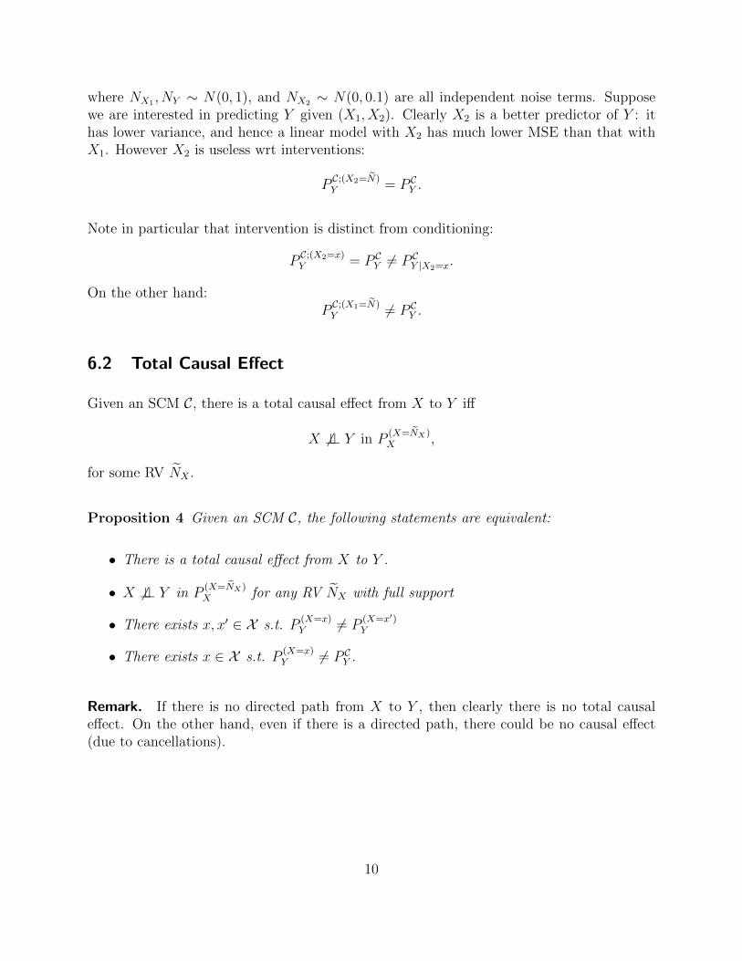
where NX1 , NY ∼ N(0, 1), and NX2 ∼ N(0, 0.1) are all independent noise terms. Supposewe are interested in predicting Y given (X1, X2). Clearly X2 is a better predictor of Y : ithas lower variance, and hence a linear model with X2 has much lower MSE than that withX1. However X2 is useless wrt interventions:

PC;(X2=N)Y = P CY .

Note in particular that intervention is distinct from conditioning:

PC;(X2=x)Y = P CY 6= P CY |X2=x.

On the other hand:PC;(X1=N)Y 6= P CY .

6.2 Total Causal Effect

Given an SCM C, there is a total causal effect from X to Y iff

X 6⊥⊥ Y in P(X=NX)X ,

for some RV NX .

Proposition 4 Given an SCM C, the following statements are equivalent:

• There is a total causal effect from X to Y .

• X 6⊥⊥ Y in P(X=NX)X for any RV NX with full support

• There exists x, x′ ∈ X s.t. P(X=x)Y 6= P

(X=x′)Y

• There exists x ∈ X s.t. P(X=x)Y 6= P CY .

Remark. If there is no directed path from X to Y , then clearly there is no total causaleffect. On the other hand, even if there is a directed path, there could be no causal effect(due to cancellations).

10

7 Pearl’s Augmented SCM

An alternate approach to specify conditional probabilities and conditional independencies inthe intervention SCM is by analyzing a augmented SCM, with an extended DAG G+.

Given an SCM C with DAG G, consider the augmented DAG G+ with parentless nodesIj pointing to each variable Xj for all j ∈ [p], where Ij ∈ no-int ∪ Xj, with Ij = no-intcorresponding to no intervention, and Ij ∈ Xj corresponding to intervening on Xj and settingit equal to Ij. One can then specify the augmented SCM C+ with structural equations:

Xj = fj(PAj(G+), Nj),

where Xj = fj(PAj, Nj)I[Ij = 0] + Ij I[Ij 6= 0].

It can then be seen that:P C

+

Y |Ij=xj= P

C;do(Xj=xj)Y .

It also follows thatP C;do(X=x)(Y ) = P C(Y |X = x),

if Y is d-separated from IX given X in the graph G+. This is because from the above:

P C;do(X=x)(Y ) = P C+

(Y |IX = x)

= P C+

(Y |IX = x,X = x)

= P C+

(Y |X = x)

= P C(Y |X = x),

where the third equality follows from the d-separation, and the last is because the marginaldistribution over the non-I variables is simply the original SCM.

We also have that:P C;do(X=x)(Y ) = P C(Y ),

if Y is d-separated from IX in the graph G+. This follows similarly:

P C;do(X=x)(Y ) = P C+

(Y |IX = x)

= P C+

(Y )

= P C(Y ),

where the second equality follows from the d-separation, and the last is because the marginaldistribution over the non-I variables is simply the original SCM.

One can extend these instances to a general calculus involving simplifying intervention con-ditionals, that Pearl called “do-calculus”.

11

7.1 Do-Calculus

As before, given an SCM C with DAG G, we can specify the augmented SCM C+ with DAGG+. Then by a simple extension of the analyses we get the following rules.

Insertion/Deletion of Observations.

P C;do(Z=z)(Y |X,W ) = P C;do(Z=z)(Y |X),

if W is d-separated from Y given IZ , X in the graph G+.

Action/Observation Exchange.

P C;do(Z=z,X=x)(Y |W ) = P C;do(Z=z)(Y |X = x,W ),

if Y is d-separated from IX given X, IZ ,W in the graph G+.

In the simplest case, with Z = W = , the above states that:

P C;do(X=x)(Y ) = P C(Y |X = x),

if Y is d-separated from IX given X in the graph G+. This is precisely what we showedearlier as a simple consequence of the d-separation.

Insertion/Deletion of Actions.

P C;do(Z=z,X=x)(Y |W ) = P C;do(Z=z)(Y |W ),

if Y is d-separated from IX given IZ ,W in the graph G+.

In the simplest case, with Z = W = , the above states that:

P C;do(X=x)(Y ) = P C(Y ),

if Y is d-separated from IX in the graph G+. This is precisely what we showed earlier as asimple consequence of the d-separation.

8 Counterfactuals

Consider an SCM C with DAG G over a random vector X. Given discrete observations x,the counterfactual SCM, denoted by CX=x is the same set of structural assignments, but

12

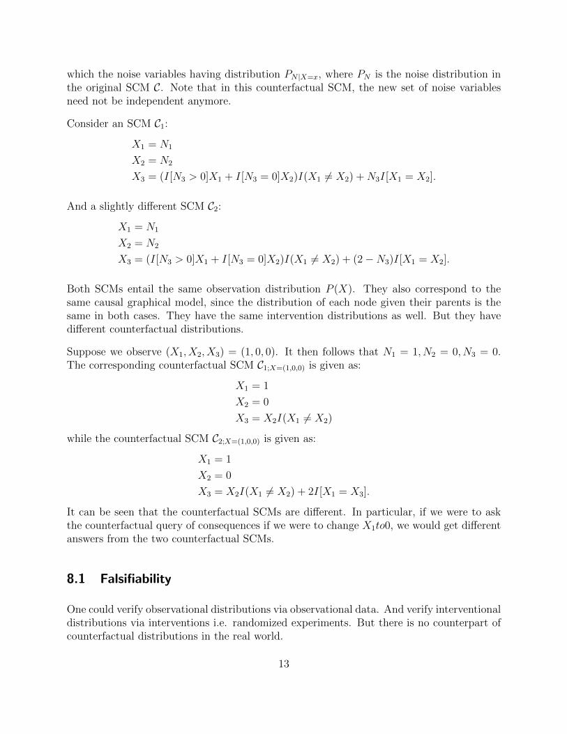
which the noise variables having distribution PN |X=x, where PN is the noise distribution inthe original SCM C. Note that in this counterfactual SCM, the new set of noise variablesneed not be independent anymore.

Consider an SCM C1:

X1 = N1

X2 = N2

X3 = (I[N3 > 0]X1 + I[N3 = 0]X2)I(X1 6= X2) +N3I[X1 = X2].

And a slightly different SCM C2:

X1 = N1

X2 = N2

X3 = (I[N3 > 0]X1 + I[N3 = 0]X2)I(X1 6= X2) + (2−N3)I[X1 = X2].

Both SCMs entail the same observation distribution P (X). They also correspond to thesame causal graphical model, since the distribution of each node given their parents is thesame in both cases. They have the same intervention distributions as well. But they havedifferent counterfactual distributions.

Suppose we observe (X1, X2, X3) = (1, 0, 0). It then follows that N1 = 1, N2 = 0, N3 = 0.The corresponding counterfactual SCM C1;X=(1,0,0) is given as:

X1 = 1

X2 = 0

X3 = X2I(X1 6= X2)

while the counterfactual SCM C2;X=(1,0,0) is given as:

X1 = 1

X2 = 0

X3 = X2I(X1 6= X2) + 2I[X1 = X3].

It can be seen that the counterfactual SCMs are different. In particular, if we were to askthe counterfactual query of consequences if we were to change X1to0, we would get differentanswers from the two counterfactual SCMs.

8.1 Falsifiability

One could verify observational distributions via observational data. And verify interventionaldistributions via interventions i.e. randomized experiments. But there is no counterpart ofcounterfactual distributions in the real world.

13

It is possible in certain cases for counterfactual distributions to be falsifiable. For instance,if we can observe the specific noise samples as entailed by the counterfactual distribution(e.g. imagine if the noise variables could be obtained via some measurement). One could alsofalsify the counterfactual SCM by drawing upon scientific theories or domain knowledge. Butin general, it is not falsifiable. That said, humans often think in terms of counterfactuals,and indeed, counterfactuals have occured in literature and philosophy throughout humanhistory. What if I was on the plane that crashed, rather than the plane that left an hourlater? What if I had picked the winning lottery numbers? And so on.

8.2 Equivalence of Causal Models

Definition 5 We say two models as probabilistically/interventionally/counterfactually equiv-alent if they entail the same obs./obs. and interv./obs., interv., and counterfactual distribu-tions.

It turns out that for a pair of positive distributions, for them to be interventionally equivalentit suffices for them to agree on simple single-node interventions where Xk = Nk for someindependent noise distribution (rather than an entirely different SCM component that coulddepend on some other subsets of nodes). This is convenient because such interventions areeasier to setup in the real world, and are also mathematically easier.

Proposition 6 Suppose that two SCMs C1, C2 with strictly positive SCM components, sat-isfy:

PC1;do(Xj=Nj)X = P

C2;do(Xj=Nj)X ,

for all j ∈ [p], and all distributions Nj with full support. Then C1 and C2 are fully interven-tionally equivalent.

9 Causal Models and DGMs

We can now revisit Reichenbach’s common cause principle in light of DGMs. Here, “causing”is taken to mean existence of a directed path. So we can restate the principle purely as aconditional independence statement in DGMs.

Proposition 7 (Reichenbach’s common cause principle: DGM Edition) If X andY are unconditionally dependent in a DGM with DAG G, then one of the statements belowis true:

1. there is a directed path from X to Y

14

2. there is a directed path from Y to X

3. there is a node Z in G with a directed path from Z to X, and from Z to Y .

Note that the above does not hold when we condition on some variable: it asks for uncon-ditional independence between X and Y . This is particularly the case when we conditionon a common child of X and Y : they would then be dependent, but none of the statementsabove would hold.

9.1 Causal Graphical Models (CGMs)

What is the difference between SCMs and CGMs? With CGMs, we only specify the distri-butions, rather than the structural equation. It is thus simply a DGM, with additionallyspecifications of interventional distributions.

Thus, given X = (X1, . . . , Xp), the CGM is specified as:

P (X) =

p∏j=1

fj(Xj, XPAj),

where fj(Xj, XPAj) = P (Xj|XPAj

.

Moreover,

P(Xk=q(·|X

PAk))

(x) =∏j 6=k

fj(Xj, XPAj)q(xk;xPAk

). (1)

Why use SCMs rather than just the set of local densities as in CGMs? They yield thesame observational distributions (as do DGMs), and the same interventional distributions,but lack the information required to specify counterfactual distributions. What if we are notinterested in counterfactual distributions? Even then, SCMs are a more natural specificationin delineating the deterministic functional components and the noise components: this isuseful in allowing for restricting just the functional or noise components for identifiabilitywhen we learn them from data, as we will see in the sequel. But at the level of observationsand interventions, and if we do not need to worry about learning/identifiability, one coulduse either formulation.

But whether we use the SCM or Causal Graphical Model form, we can simply derive theintervention distribution as in (1), by just replacing one of the factors with that specifiedby the intervention. This is known by various names: truncated factorization (Pearl 1993),G-computation (Robins 1986), and manipulation theorem (Spirtes 2000). It is worth re-iterating this facet of CGMs/SCMs: we can obtain intervention distributions from themwithout observing data specifically from these interventions.

15

10 SCM Calculus

While the truncated factorization in (1) specifies a new intervention SCM, and one wouldneed to perform probabilistic reasoning on this new SCM to derive conditional probabilitiesof interest. But could we directly express the conditional probabilities in the interventionSCM in terms of conditional probabilities in the original SCM?

Definition 8 (Confounding) Consider an SCM C, with a directed path from X to Y , forsome nodes X, Y ∈ V . The causal effect from X to Y is said to be confounded if:

P C;do(X:=x)(y) 6= P C)(y).

Otherwise the causal effect is said to unconfounded.

Thus, there exist some confounding variables that account for the dependence between Xand Y . Consider the following simple instance of such confounding.

Example 9 (Kidney Stones) Suppose somebody has kidney stones for which they seektreatment. Let Z be a RV that denotes the size of the kidney stones, T a binary treatmentRV (with T = 0 indicating one treatment, and T = 1indicating the other), and R a binaryrecovery RV (with R = 1 indicating recovery, and R = 0 otherwise.) We are interested inmeasuring the average causal effect between the treatments:

P C;do(T=1)(R = 1)− P C;do(T=2)(R = 1).

Note that this is different from the difference between the conditionals:

P C(R = 1|T = 1)− P C(R = 1|T = 2).

But we can connect some conditionals in P C;do(T=t) to conditionals in P C. For instance, itcan be seen from inspecting the intervention SCM that:

P C;do(T=1)(R = 1|T = 1, Z = z) = P C(R = 1|T = 1, Z = z)P C;do(T=1)(Z = z) = P C(Z = z)

This thus allows us to perform the following calculation:

P C;do(T=1)(R = 1) =∑z

P C;do(T=1)(R = 1, T = 1, Z = z)

=∑z

P C;do(T=1)(R = 1|T = 1, Z = z)P C;do(T=1)(T = 1, Z = z)

=∑z

P C;do(T=1)(R = 1|T = 1, Z = z)P C;do(T=1)(Z = z)

=∑z

P C(R = 1|T = 1, Z = z)P C(Z = z),

16

In the example above, by adjusting for Z, we could compute the effect of the treatmententirely from observational conditional probabilities. This leads us to the following concept.

Definition 10 (Valid Adjustment Set) Consider an SCM C, and two nodes X, Y ∈ V ,where Y 6∈ paX . We call a set Z a valid adjustment set for the ordered pair (X, Y ) if:

P C;do(X:=x)(y) =∑z

P C)(y|x, z)P C(z).

Let us now perform a calculation similar to the kidney stones example. For any set of nodesZ ⊆ V , we have that:

P C;do(X:=x)(y) =∑z

P C;do(X:=x)(y, z)

=∑z

P C;do(X:=x)(y|x, z)P C;do(X:=x)(z).

So, if the set of nodes Z satisfies:

P C;do(X:=x)(y|x, z) = P C(y|x, z)

P C;do(X:=x)(z) = P C(z), (2)

it then follows that Z is a valid adjustment set. We now need to characterize when such asubset of nodes Z will be invariant to interventions on X. As in an earlier section, considerthe extended DGM G+ corresponding to the SCM with intervention indicator variables IXcorresponding to variables X. It then follows that (2) is satisfied if:

Y ⊥⊥G+ IX |X,ZZ ⊥⊥G+ IX . (3)

Now, suppose Z ′ ∈ V s.t.

Z ′ ⊥⊥ Y |X,Z. (4)

Then:∑z,z′

P C;do(X:=x)(y|x, z, z′)P C;do(X:=x)(z, z′) =∑z

P C;do(X:=x)(y|x, z)∑z′

P C;do(X:=x)(z, z′)

=∑z

P C;do(X:=x)(y|x, z).

It thus follows that for any Z satisfying (3), Z ′ satisfies (4) wrt that Z, then Z∪Z ′ is alsoa valid adjustment set.

Proposition 11 (Shpitser et al, 2010) Consider an SCM C. Any Z that satisfies (3) is avalid adjustment set for X, Y ∈ V . Given a valid adjustment set Z, suppose Z ′ satisfies (4)wrt Z. Then Z ∪ Z ′ is also a valid adjustment set. These are the only valid adjustmentsets.

17

11 Potential Outcomes

Suppose that X is a binary variable that represents some exposure. So X = 1 meansthe subject was exposed and X = 0 means the subject was not exposed. And Y is some“outcome” variable measuring how well the treatment worked.

We can address the problem of predicting Y from X by estimating P (Y |X = x). But thatdoes not get at causal dependence between X and Y . Let Y1 denote the response if thesubject is exposed. Let Y0 denote the response if the subject is not exposed. If we exposea subject, we observe Y1 but we do not observe Y0. Instead, Y0 is the value we would haveobserved if the subject had NOT been exposed.

Thus,

Y =

Y1 if X = 1

Y0 if X = 0.

More succinctlyY = XY1 + (1−X)Y0. (5)

The variables (Y0, Y1) are also called potential outcomes.

We have replaced the random variables (X, Y ) with the more detailed variables (X, Y0, Y1, Y )where Y = XY1 + (1−X)Y0.

A small dataset might look like this:

X Y Y0 Y1

1 1 * 11 1 * 11 0 * 01 1 * 10 1 1 *0 0 0 *0 1 1 *0 1 1 *

It is important to keep in mind here that each row corresponds to a different subject. Thus,X = 1 in any row indicates that subject was given the treatment, and X = 0 indicatesthey were not. The asterisks indicate unobserved variables. So, for those subjects for whomX = 1, for those specific subjects, we only observe their Y1 value, and do not observe theirY0 value.

Causal questions involve the the distribution P (Y0, Y1) of the potential outcomes. For in-stance, the treatment could be said to be effective if E[Y1]− E[Y0] is large.

18

Thus, in the potential outcomes view, causal analysis involves reasoning about some randomvariables — potential outcomes — which by definition are rife with missingness. How do werelate this to causal SCMs, and the causal graph approach we have studied so far?

Given an SCM C, we can interpret Y1 as Y C;do(X=1) and Y0 as Y C;do(X=0) We can verify thatfor any SCM C:

Y C = Y C;do(X=1)I[XC = 1] + Y C;do(X=0)I[XC = 0].

But there are other interpretations as well, since the potential outcomes literature focuseson individual subjects. Pearl (2009) thus suggests that any individual subject u can beassociated with some noise variables Nu, so that we can consider the resulting counterfactualSCM CN=Nu . The potential outcomes for subject u can then be specified as:

Y0(u) = Y CN=Nu ;(X=0)

Y1(u) = Y CN=Nu ;(X=1),

but specializes our earlier specification to an individual for whom treatment outcomes forinstance could be deterministic.

But even if you find this specific connection convoluted, it is instructive to look at howpotential outcomes are measured given data.

One approach is to use a randomized trial, where we ensure that X ⊥⊥ (Y0, Y1): sincewho gets treatment is chosen completely independently (for instance by uniformly randomassignment) of how they may fare given the treatment. We can then simply write: P (Y1) =P (Y1|X = 1) = P (Y |X = 1). And similarly, P (Y0) = P (Y |X = 1), so that we couldestimate the potential outcome probabilities just from conditionals over the observed RVs.This is why randomized control trials are used for measuring causal effects.

But suppose X was not chosen independent of Y0, Y1, for instance, we only had access toobservational data. But suppose we knew all the “confounding” variables Z such that:

X ⊥⊥ (Y0, Y1) |Z(Z0,Z1) ∼d Z

Thus conditioned on the confounding variables, the treatment outcomes are independent ofwho gets the treatment. An example of such confounding variables could be age, or socio-economic status. We also assume that intervening on the treatment would not have affectedthe distribution of the confounding variables (e.g. we would not affect the age by deciding

19

to give somebody the treatment!). Given such a confounding set, we then have:

P (Y1) =∑z

P (Y1|Z1 = z)P (Z1 = z)

=∑z

P (Y1|X = 1,Z1 = z)P (Z = z)

=∑z

P (Y |X = 1, Z = z)P (Z = z),

where the second equality used the independence of X, as well as that Z1 ∼d Z, while the lastequality simply used the definition of potential outcomes. This can be seen to be preciselythe computation using a valid adjustment set, and the conditions above are precisely thosespecifying valid adjustment sets. Thus, causal SCMs and potential outcomes result in thesame calculations under the same assumptions.

One can even show that theorems that hold in one framework also hold under equivalentassumptions in the other framework. Nonetheless, they might be easier to prove in oneframework vs the other. Potential outcomes seem preferable for a smaller set of discretevariables, while SCMs might be preferable for larger scale settings. Potential outcomes alsofocus on assumptions that relate interventional quantities to observed conditionals, whileSCMs allow for more complex causal reasoning.

12 Algorithmic Notion of Causality

So far we have discussed conditional independence properties among random variables. Butif we are to ask that causal mechanisms i.e. conditional distributions of nodes given theirparents are to be “independent,” it might seem we lack the technical tools to define whatwe mean when we say that two conditional distributions (in contrast to random variables)are independent.

Consider objects (not necessarily random variables) from some set Ω. And assume that wehave access to an “information” functional:

R : 2Ω 7→ R,

that given a set of objects, can quantify the amount of information in this set. For any twosets x,y ⊆ Ω, we would have that: R(x,y) ≥ R(y), so that R is monotone. We could thusinterpret: R(x |y) = R(x,y)− R(y) as the conditional information in x given y. Similarlywe can define a counterpart of mutual information:

I(x; y) = R(x) +R(y)−R(x,y),

as well as conditional mutual information:

I(x; y | z) = R(x, z) +R(y, z)−R(x,y, z)−R(z).

20

We can also define generalized SCMs over a set of objects (x1, . . . , xp) by requiring that anode xj not contain more information than its parents paj and an unobserved independentnoise object nj:

R(xj,paj, nj) = R(paj, nj),

and further that the noise objects are independent:

R(n1, . . . , np) =

p∑j=1

R(nj).

This can also be stated simply as:

I(n1, . . . , np) = 0.

Janzing and Scholkopf (2010) suggest the use of Kolmogorov complexity as the notion ofinformation above, to derive an “algorithmic model of causality”. This might be suitable tocases where the data consists of non-stationary perhaps even deterministic time-series, forwhich such algorithmic notions of dependence might be better suited.

12.1 Algorithmic Independence of Conditionals

Given such an algorithmic notion of dependence, we can now formalize one notion of “in-dependence” of causal mechanisms. We say that an SCM has algorithmically independentconditionals if:

I(PX1 |PA1 , . . . , PXp |PAp) = 0.

References

Elements of Causal Inference, Foundations and Learning Algorithms, Jonas Peters, Do-minik Janzing and Bernhard Scholkopf, available for free: https://www.dropbox.com/s/

gkmsow492w3oolt/11283.pdf?dl=1

Causal Inference, Miguel Hernan, also available for free: https://www.hsph.harvard.edu/miguel-hernan/causal-inference-book/

21