Caste, Female Labor Supply and the Gender Wage Gap in India:

Boserup Revisited

Kanika Mahajan

Bharat Ramaswami*

October 2012

ABSTRACT

A look at the spatial variation in male and female agricultural wages in India throws up a

seeming paradox: gender differentials are the largest in the southern regions of India that are

otherwise favourable to women. Boserup (1970) hypothesized that this is due to the greater

labor force participation of women in these regions. This is not obvious as greater female

labor supply could depress male wages as well. This paper undertakes a formal test of the

Boserup proposition. Econometrically, the main challenge is to relate wages to exogenous

variation in labor supply. The results show that differences in female labor supply are able to

explain 55% of difference in gender wage differential between northern and southern states

of India. Key words: Wage gap, Female, Agriculture, Labor supply, Caste JEL Codes: J21, J22, J31, J16, J43, O15

___________________________ * Indian Statistical Institute, Delhi. Email: kanika9r@isid.ac.in and bharat@isid.ac.in

We thank Vegard Iversen and Kensuke Kubo for comments on an earlier draft. We also thank Richard Palmer-

Jones for providing the data on agro-ecological zone composition at the district level used in this paper.

1

Caste, Female Labor Supply and the Gender Wage Gap in India:

Boserup Revisited

1. Introduction

The gender gap in wages is a widely documented phenomenon. Though many

countries have passed minimum wage laws and laws mandating equal treatment of women at

workplace, gender wage differential remains a persistent feature of labor markets. The

standard wage discrimination analysis would suggest that the variation in the gender gap is

due to `explainable’ differences in observed characteristics and endowments and the variation

in `unexplained’ differences commonly attributed to wage discrimination. However, in a

cross-country context, observable differences in characteristics and endowments, explain

only a small portion of the wage gap (Hertz et. al, 2009). Female wages as a percentage of

male wages is close to 100% in parts of Latin America and Kenya but can be just above 50%

in Afghanistan and parts of South Asia. Since the unexplained component is the dominant

one, the geographical variation in the wage gap is essentially unexplained.

Variation in gender wage gaps can be observed within a country as well. On average

female daily wage rate in agriculture is 70% of that of male agricultural labor in India

(National Sample Survey, 2004). However, there are wide differences across states ranging

from 90% in the state of Gujarat to 54% in Tamil Nadu. Explaining the spatial variation in

India is the goal of this paper. In particular, the paper asks whether exogenous variation in

female and male labor supply to agriculture play any part in causing the gender wage gap.

The relationship between female labor supply and the gender wage gap has been investigated

in developed countries as well. Acemoglu (2004) considered the increased work

participation of women to explain the post-World War II increase in the gender wage gap in

the United States. Blau and Kahn (2003) study the relation in a 22 country sample drawn

mostly from the OECD countries.

2

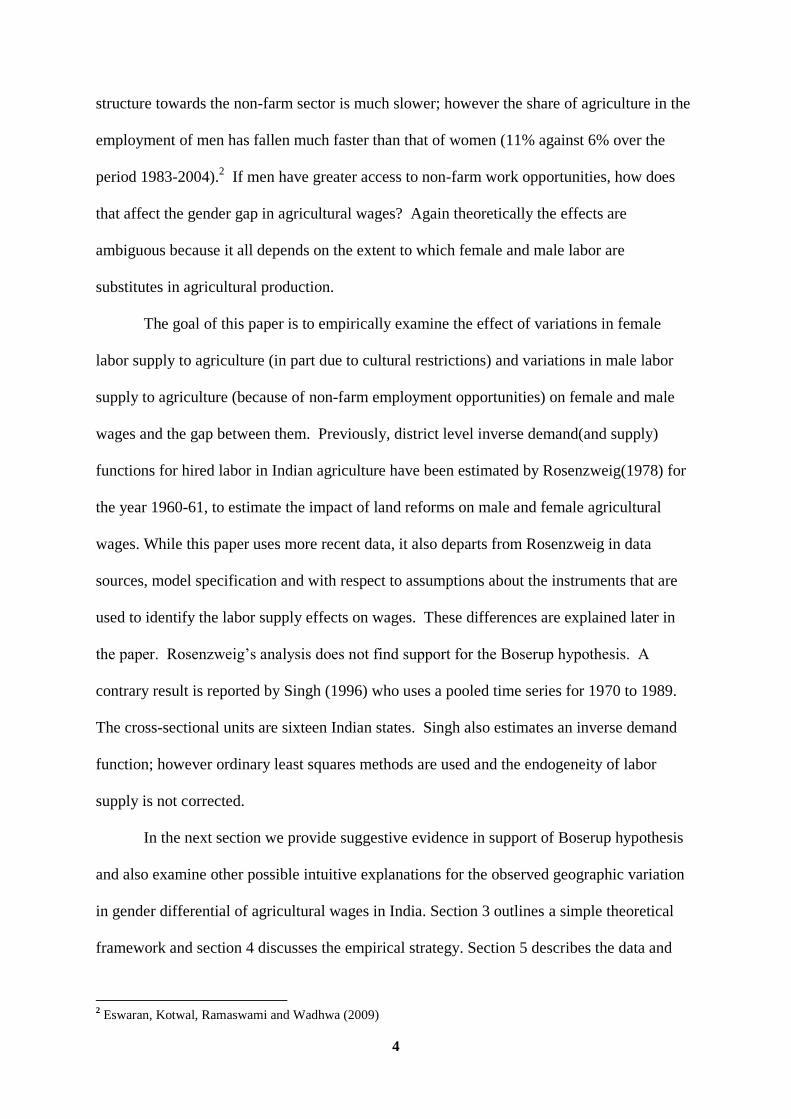
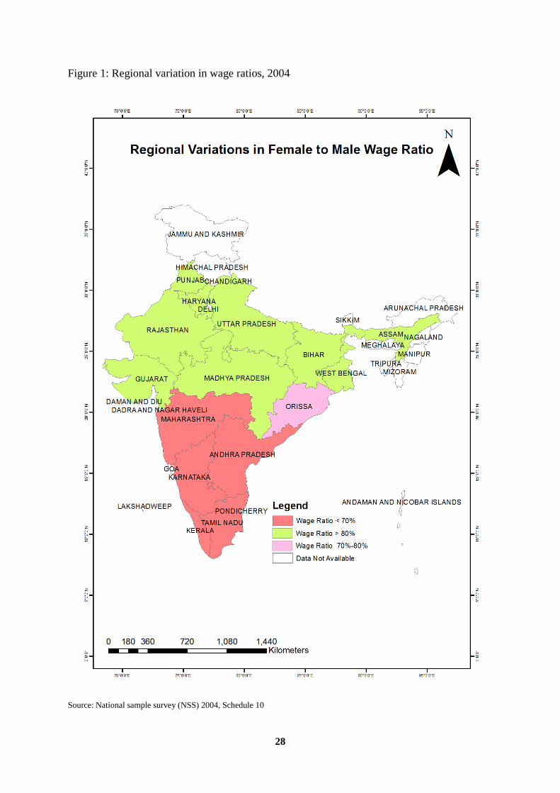
Figure 1 maps the gender differential in agricultural wages across states in India. On a

closer inspection one can observe a systematic regional pattern- gender gap in wages in the

northern states is much lower than in the southern states. At a first glance this seems to be

against a well known finding that women have greater autonomy in the southern states

(Dyson and Moore, 1983). Basu (1992) and Jejeebhoy (2001) also find similar patterns in

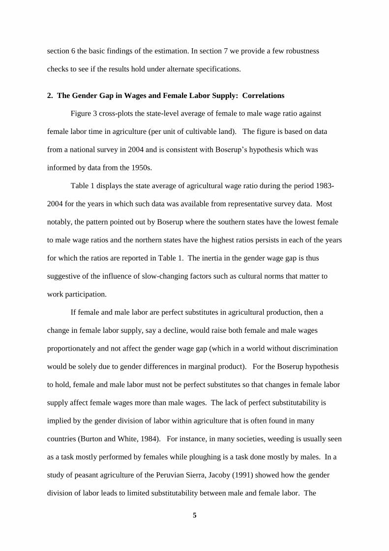
woman’s status indicators in a society across India’s north and south.1 The panels in Figure

2 cross-plot the female to male wage ratio against some commonly used indicators of the

welfare of women – the sex ratio in the population, the percentage of women with a body

mass index below the threshold of 18.5, the percentage of women who have experienced

physical or sexual violence, the percentage of women who can make decisions regarding

social visits, major household purchases and the percentage of women who can travel

unaccompanied to the market, health facility and destinations outside the village. It can be

seen that regions with greater gender wage gaps are, in fact, characterized by indicators that

are favorable to women.

An explanation of this apparent paradox is provided by Boserup (1970). She posits

that the variation in gender wage differential across states is because of variation in female

labor supply. Female labor force participation is much higher in the southern states than in

the north. This characteristic of the labor market has been well studied (e.g. Nayyar(1987),

Chen(1995), Bardhan(1984) and Das(2006)). The variation in female labor force

participation in some studies is attributed to varying agro-ecological conditions in India, for

instance, wet-rice farming traditionally employs more female labor (Agarwal, 1986).

Boserup’s argument, however, revolves around the cultural restrictions on woman’s

participation in work and the variation in this norm across India. Boserup points out that,

typically, higher caste Hindu women take no part in cultivation activities while tribal and low

1 However, Rahman and Rao (2003) do not find such a distinct differentiation across all indicators of woman’s

status.

3

caste women have traditions of female farming either on their own land or as wage labor.

She also points out that tribal and low caste populations are lower in north India relative to

other parts of the country. The association of social group membership (caste and tribe) with

female work participation has been confirmed in later work as well (e.g., Chen (1995), Das

(2006), Eswaran, Ramaswami and Wadhwa (2012)). Boserup follows up these observations

with its consequences. In her words,

“The difference between the wages paid to women and to men for the same agricultural tasks

is less in many parts of Northern India than is usual in Southern India and it seems reasonable

to explain this as a result of the disinclination of North Indian women to leave the domestic

sphere and temporarily accept the low status of an agricultural wage laborer.” (Boserup, p

61).

Boserup’s hypothesis is based on raw correlations drawn from wage data across

villages in different Indian states in the 1950s. However, the hypothesis is not immediately

obvious because variations in female labor supply could affect male wages as well. Indeed,

theoretically, the effects are ambiguous (Rosenzweig, 1978). Furthermore, there could be

other factors that affect the gender wage gap as well. Firstly, the analysis should account for

gender segregation by task where `female’ tasks are possibly paid less than supposedly

`male’ tasks. Secondly, the efficiency of male and female labor in agriculture could vary

across regions because of differences in cropping pattern and agro-climatic condition and

these need to be controlled for. Thirdly, factors which affect supply of male labor to

agriculture like non-farm employment could also matter to the wage gap. It is well known

that the labor flow from agriculture to other sectors has been much more marked for males

than for females (Eswaran et.al, 2009). If the trends in any of these factors vary by state then

this must also be reckoned as a possible explanation.

Indeed, the impact of non-farm employment on the gender wage gap is of independent

interest as well. The non-farm sector is growing much faster than the farm sector as a result

of which agriculture’s share in GDP has dipped below 20%. The shift in the employment

4

structure towards the non-farm sector is much slower; however the share of agriculture in the

employment of men has fallen much faster than that of women (11% against 6% over the

period 1983-2004).2 If men have greater access to non-farm work opportunities, how does

that affect the gender gap in agricultural wages? Again theoretically the effects are

ambiguous because it all depends on the extent to which female and male labor are

substitutes in agricultural production.

The goal of this paper is to empirically examine the effect of variations in female

labor supply to agriculture (in part due to cultural restrictions) and variations in male labor

supply to agriculture (because of non-farm employment opportunities) on female and male

wages and the gap between them. Previously, district level inverse demand(and supply)

functions for hired labor in Indian agriculture have been estimated by Rosenzweig(1978) for

the year 1960-61, to estimate the impact of land reforms on male and female agricultural

wages. While this paper uses more recent data, it also departs from Rosenzweig in data

sources, model specification and with respect to assumptions about the instruments that are

used to identify the labor supply effects on wages. These differences are explained later in

the paper. Rosenzweig’s analysis does not find support for the Boserup hypothesis. A

contrary result is reported by Singh (1996) who uses a pooled time series for 1970 to 1989.

The cross-sectional units are sixteen Indian states. Singh also estimates an inverse demand

function; however ordinary least squares methods are used and the endogeneity of labor

supply is not corrected.

In the next section we provide suggestive evidence in support of Boserup hypothesis

and also examine other possible intuitive explanations for the observed geographic variation

in gender differential of agricultural wages in India. Section 3 outlines a simple theoretical

framework and section 4 discusses the empirical strategy. Section 5 describes the data and

2 Eswaran, Kotwal, Ramaswami and Wadhwa (2009)

5

section 6 the basic findings of the estimation. In section 7 we provide a few robustness

checks to see if the results hold under alternate specifications.

2. The Gender Gap in Wages and Female Labor Supply: Correlations

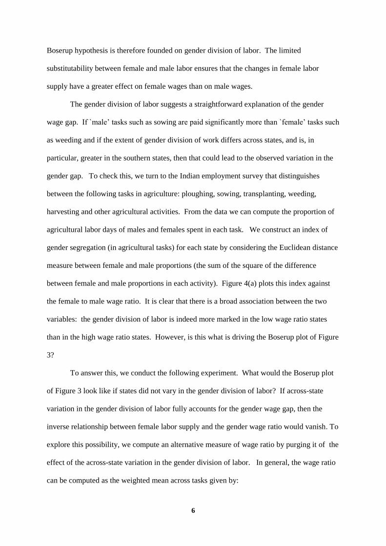
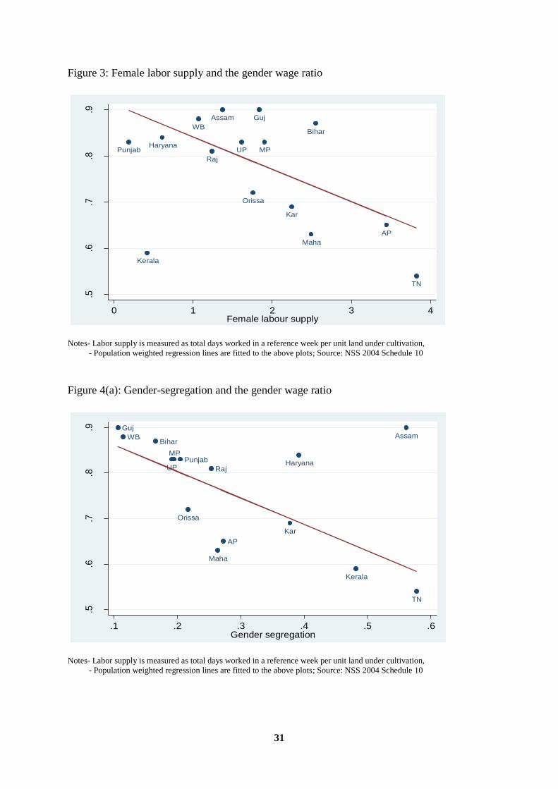
Figure 3 cross-plots the state-level average of female to male wage ratio against

female labor time in agriculture (per unit of cultivable land). The figure is based on data

from a national survey in 2004 and is consistent with Boserup’s hypothesis which was

informed by data from the 1950s.

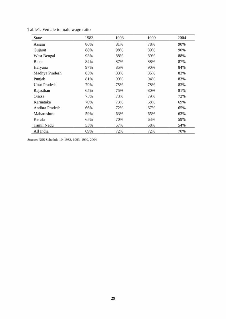
Table 1 displays the state average of agricultural wage ratio during the period 1983-

2004 for the years in which such data was available from representative survey data. Most

notably, the pattern pointed out by Boserup where the southern states have the lowest female

to male wage ratios and the northern states have the highest ratios persists in each of the years

for which the ratios are reported in Table 1. The inertia in the gender wage gap is thus

suggestive of the influence of slow-changing factors such as cultural norms that matter to

work participation.

If female and male labor are perfect substitutes in agricultural production, then a

change in female labor supply, say a decline, would raise both female and male wages

proportionately and not affect the gender wage gap (which in a world without discrimination

would be solely due to gender differences in marginal product). For the Boserup hypothesis

to hold, female and male labor must not be perfect substitutes so that changes in female labor

supply affect female wages more than male wages. The lack of perfect substitutability is

implied by the gender division of labor within agriculture that is often found in many

countries (Burton and White, 1984). For instance, in many societies, weeding is usually seen

as a task mostly performed by females while ploughing is a task done mostly by males. In a

study of peasant agriculture of the Peruvian Sierra, Jacoby (1991) showed how the gender

division of labor leads to limited substitutability between male and female labor. The

6

Boserup hypothesis is therefore founded on gender division of labor. The limited

substitutability between female and male labor ensures that the changes in female labor

supply have a greater effect on female wages than on male wages.

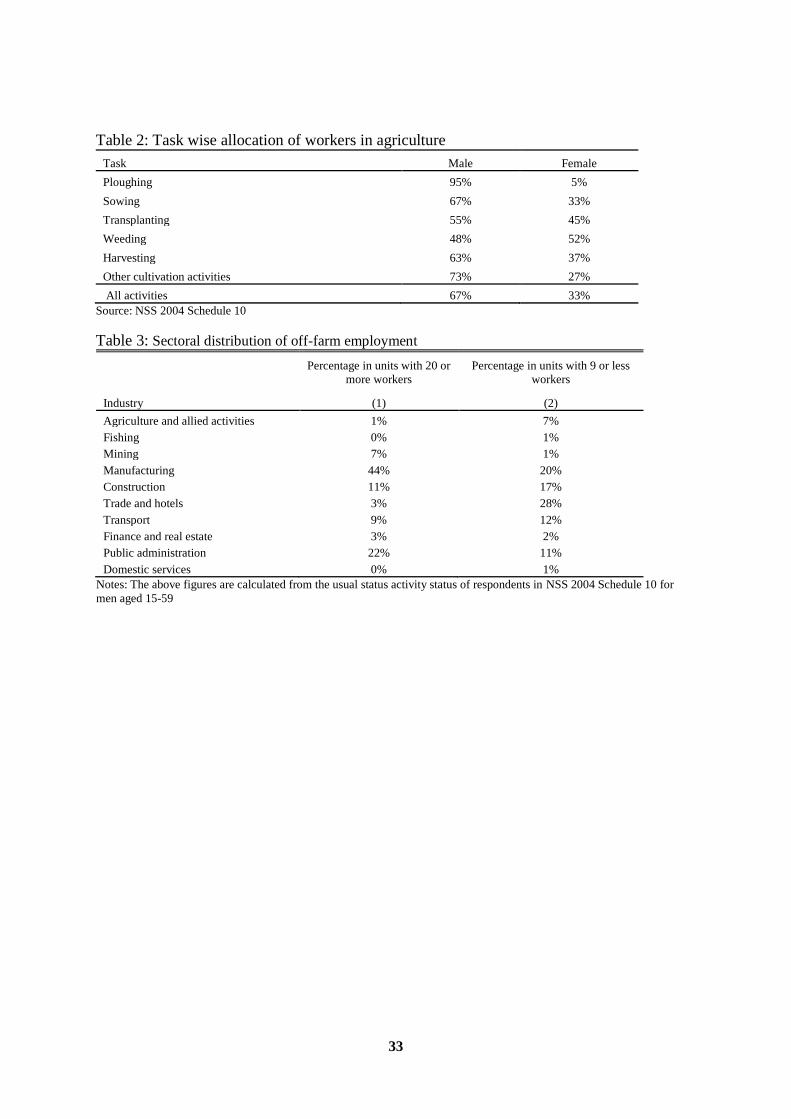
The gender division of labor suggests a straightforward explanation of the gender

wage gap. If `male’ tasks such as sowing are paid significantly more than `female’ tasks such

as weeding and if the extent of gender division of work differs across states, and is, in

particular, greater in the southern states, then that could lead to the observed variation in the

gender gap. To check this, we turn to the Indian employment survey that distinguishes

between the following tasks in agriculture: ploughing, sowing, transplanting, weeding,

harvesting and other agricultural activities. From the data we can compute the proportion of

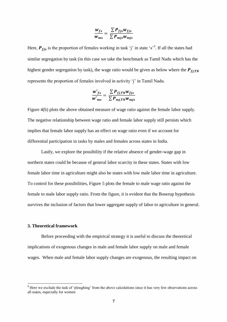
agricultural labor days of males and females spent in each task. We construct an index of

gender segregation (in agricultural tasks) for each state by considering the Euclidean distance

measure between female and male proportions (the sum of the square of the difference

between female and male proportions in each activity). Figure 4(a) plots this index against

the female to male wage ratio. It is clear that there is a broad association between the two

variables: the gender division of labor is indeed more marked in the low wage ratio states

than in the high wage ratio states. However, is this what is driving the Boserup plot of Figure

3?

To answer this, we conduct the following experiment. What would the Boserup plot

of Figure 3 look like if states did not vary in the gender division of labor? If across-state

variation in the gender division of labor fully accounts for the gender wage gap, then the

inverse relationship between female labor supply and the gender wage ratio would vanish. To

explore this possibility, we compute an alternative measure of wage ratio by purging it of the

effect of the across-state variation in the gender division of labor. In general, the wage ratio

can be computed as the weighted mean across tasks given by:

7

Here, is the proportion of females working in task ‘j’ in state ‘s’3. If all the states had

similar segregation by task (in this case we take the benchmark as Tamil Nadu which has the

highest gender segregation by task), the wage ratio would be given as below where the

represents the proportion of females involved in activity ‘j’ in Tamil Nadu.

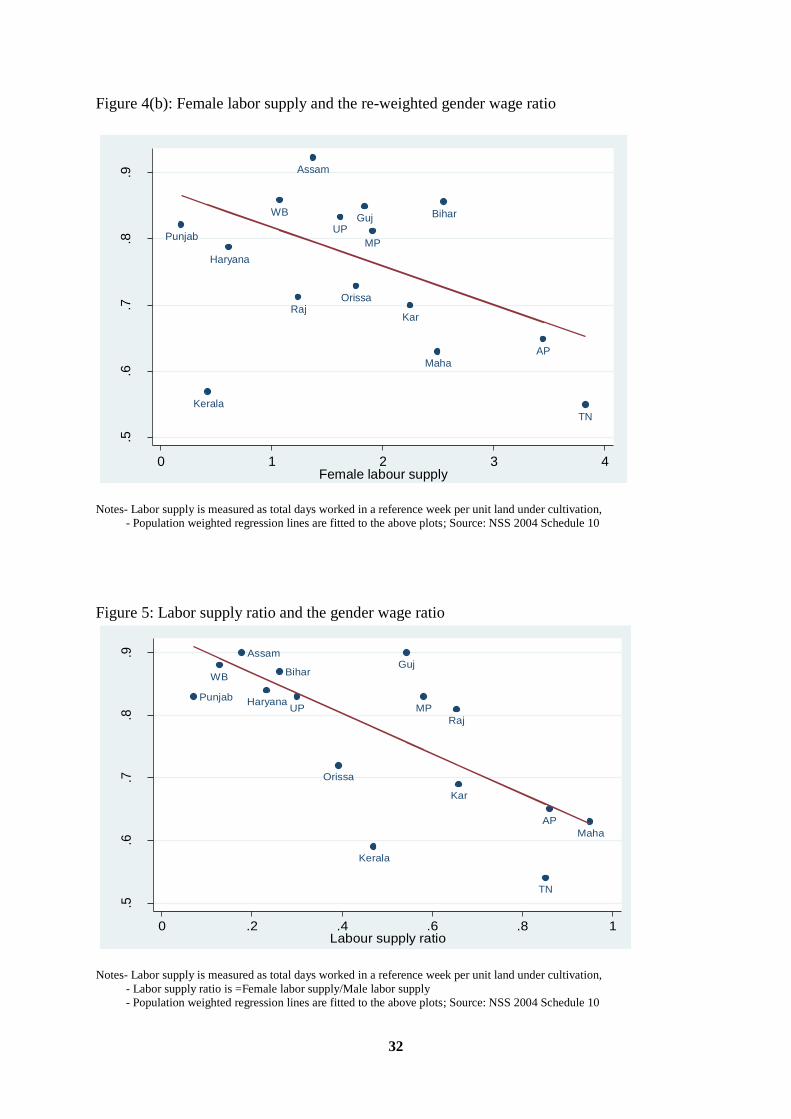
Figure 4(b) plots the above obtained measure of wage ratio against the female labor supply.

The negative relationship between wage ratio and female labor supply still persists which

implies that female labor supply has an effect on wage ratio even if we account for

differential participation in tasks by males and females across states in India.

Lastly, we explore the possibility if the relative absence of gender-wage gap in

northern states could be because of general labor scarcity in these states. States with low

female labor time in agriculture might also be states with low male labor time in agriculture.

To control for these possibilities, Figure 5 plots the female to male wage ratio against the

female to male labor supply ratio. From the figure, it is evident that the Boserup hypothesis

survives the inclusion of factors that lower aggregate supply of labor to agriculture in general.

3. Theoretical framework

Before proceeding with the empirical strategy it is useful to discuss the theoretical

implications of exogenous changes in male and female labor supply on male and female

wages. When male and female labor supply changes are exogenous, the resulting impact on

3 Here we exclude the task of ‘ploughing’ from the above calculations since it has very few observations across

all states, especially for women

8

wages can be determined by reading off the labor demand curve. Identification of such

exogenous changes and the estimation of the demand curve is the subject of later sections.

In the model below we assume competitive agricultural labor market with

exogenously determined labor supply and three factors of production – Land (A), Male labor

(Lm) and Female labor (Lf). The production function is homogenous, continuous and

differentiable. There exist diminishing returns to each factor and in the short run the amount

of land is fixed. The profit function is given by:

In a competitive equilibrium all factors are paid their marginal products. Let and

denote the marginal product of male and female labor respectively. The first order

conditions for labor demand satisfy

(1)

(2)

From these, the own and cross price elasticities of male wages to exogenous changes in labor

supply can be derived as the following.

Similar, expressions for own and cross price elasticity of female wages to exogenous changes

in labor supply are given by

9

The diminishing returns to factors inputs imply that own price elasticity’s, (3) and (5) are

negative. To sign the cross wage elasticity we need to know whether male and female labor

are substitutes or complements in the production process. If they are imperfect substitutes

then (4) and (6) will also be negative since marginal product of male labor will decline if

female labor increases and vice versa. If they are complements then (4) and (6) will be

positive.

The effect of female labor supply on the gender wage gap is given by

-

. If male and female labor are substitutes (whether perfect or not), this

expression cannot be signed without further restrictions. If the two kinds of labor are

complements, then increase in female labor supply will increase the gender wage gap.

Similarly, the effect of male labor supply on the gender wage gap is given by

.

Again, this expression cannot be signed when male and female labor are substitutes. If they

are complements, then an increase in the male labor supply will reduce the gender wage gap.

Note that the relative magnitude of the cross wage elasticities can be obtained from (4) and

(6). This is given by

The relative magnitude of the cross price elasticities can thus be expressed as a product of

male to female labor supply and male to female wage ratio. In the Indian agricultural labor

market, it is seen that the labor supply of males is greater than that of females and the male

wage is also greater than female wage. Therefore, the above expression will be greater than

10

unity which implies that the effect of male labor supply on female wage will be greater than

the effect of female labor supply on male wage. Later, in the paper we see if the estimate of

the relative cross price elasticities implied by the above theoretical model holds ground

empirically.

4. Empirical strategy

For observed levels of female and male employment in agriculture, the inverse

demand functions can be written as

where k = F, M indexes female and males respectively, i indexes district, W is log of real

wage, L is log of labor employed in agriculture, X are other control variables. The inverse

demand functions are estimated at the level of a district. This requires Indian districts to

approximate separate agricultural labor markets. Previous studies such as those by

Jayachandran (2006) and Rosenzweig (1978) also make a similar assumption. If migration

makes the entire country a single labor market then there would be no observed relationship

between district employment and district wages as wages would equalize across districts.

However, it is well known that migration across districts is low in India. Census data show

that intra-state flows dominate this low rate and more than half of intra-state migration is

accounted by intra-district flows from rural to rural areas (Mitra and Murayama, 2008).

Moreover, marriage related migration by females dominate permanent migration streams.

Seasonal migration estimates from the National Sample Survey, 2007 in India also show that

5% of rural men and less than 1% of rural women undertake seasonal migration for

alternative employment in a year and even among these 70% migrate to urban areas for non-

11

agricultural jobs. Thus, the assumption that districts act as closed agricultural labor markets

does not seem unreasonable in the light of the above facts.

The key data used in this paper is from the nationally representative Employment and

Unemployment survey of 2004/05 conducted by National Sample Survey (NSS)4. The survey

contains labor force participation and earnings details for the reference period of a week and

follows a two stage sampling design. In the rural areas, the first stratum is a district. Villages

are primary sampling units (PSU) and are picked randomly in the district and the households

are randomly chosen in the selected PSU’s. A total of 79, 306 households are surveyed in the

rural areas. The analyses includes 15 major states in the sample: Punjab, Haryana, Uttar

Pradesh(includes Uttarakhand), Madhya Pradesh (includes Chattisgarh), Bihar (includes

Jharkhand), Gujarat, Rajasthan, Assam, West Bengal, Maharashtra, Andhra Pradesh,

Karnataka, Orissa, Tamil Nadu and Kerala.

From (1) and (2), it can be seen that the effect of female labor supply on the gender

gap in agricultural wages is given by (α1 – α0). As α1 is expected to be negative, an increase

in female labor supply leads to a greater gender gap in agricultural wages (i.e., the Boserup

hypothesis) if (α1 – α0) < 0. Similarly, the effect of male labor supply on the gender gap in

agricultural wages is (β1 – β0). A decline in male labor supply to agriculture due to greater

non-farm employment opportunities would increase the gender gap in agricultural wages if

(β1 – β0) > 0. Identification requires that we relate wages to exogenous variation in female

and male labor supply to agriculture. What instrument variables could identify such

exogenous variation?

4 There are primarily two sources for district level agricultural wages- Agricultural wages in India (AWI) and

Employment and Unemployment schedule of the National Sample Survey in India. The problem with AWI is

that no standard procedure is followed by states as the definition of “wage” is ambiguous. Also, just one village

is required to be selected in a district for the purpose of reporting of wage data. See Rao (1972) and Himanshu

(2005) for discussion about the merits of different sources of data. The consensus is that although the AWI data

may work well for long-term trend analyses it is not suitable for a cross sectional analyses if the data biases

differ across states.

12

For female labor supply, this paper uses the proportion of district population that is

low caste as an instrument. Earlier work has established the effect of caste on female labor

supply. As remarked earlier, sociologists have observed that high caste women refrain from

work participation because of `status’ considerations (Aggarwal, 1994; Beteille, 1969;

Boserup, 1970; Chen, 1995). These observations from village level and local studies have

been confirmed by statistical analysis of large data sets. Using nationally representative

employment data, Das (2006) showed that castes ranking higher in the traditional caste

hierarchy have consistently lower participation rates for women. The `high’ castes also have

higher wealth, income and greater levels of education. So could the observed effect be due

only to the income effect (although the greater education levels among higher castes should

work in the opposite direction)? In an empirical model of household labor supply, Eswaran,

Wadhwa and Ramaswami (2012) showed that `higher’ caste households have lower female

labor supply even when there are controls for male labor supply, female and male education,

family wealth, family composition, and village level fixed effects that control for local labor

market conditions (male and female wages) as well as local infrastructure.

The exclusion restriction is that caste composition affects wages only through its

affect on labor supply of women to agriculture. Could the caste composition of a district

directly affect the demand for agricultural labor? Rajaraman (1986) and Das and Dutta

(2007) find no evidence of discrimination against lower castes in the casual rural labor

market in India. If, however, the caste composition is correlated with developmental

indicators that affect agricultural technology then it could have an indirect impact on demand

for labor. Such a correlation could arise from public and private investments. For instance,

Banerjee and Somanathan (2007) find that districts with greater tribal population have less

access to public goods due to their limited political clout. This would mean that the

proportion of district proportion that is low caste would be a suitable instrument if it is

13

conditioned on development indicators such as irrigation, education, access to roads,

commercial banks and electricity. Binswanger et al (1993) find that infrastructure

investments affect agricultural productivity and agro-climatic conditions play a very

important role in determining the public and private infrastructure investment decisions.

Controlling for agro-ecological conditions is thus critical as they affect agriculture production

technology directly and indirectly by affecting the placement of public goods.

Another possibility is that the caste composition in a district reflects long run

development possibilities. In this story, the `higher castes’ used their dominance to settle in

better endowed regions. Once again, this would call for adequate controls for agro-ecological

conditions. Finally, could caste composition itself be influenced by wages? Anderson (2011)

argues that village level caste composition in India has remained unchanged for centuries and

the location of castes is exogenous to current economic outcomes. This is, of course, entirely

consistent with the low levels of mobility noted earlier.

Turning to male labor supply to agriculture, the paper uses a measure of the presence

of the non-farm economy as an instrument. The competition from non-farm jobs reduces the

labor supply to agriculture and increases wages. Evidence on this relation has been presented

by Lanjouw and Murgai (2009). Rosenzweig’s (1978) study of agricultural labor markets

also uses indicators of non-farm economy as an instrument for labor supply to agriculture.5

However, non-farm activity could in general be endogenous to the agricultural labor market.

In this paper, a variable measuring non-farm employment in large work manufacturing and

mining units is used as an instrument for male labor supply. As we shall argue, such a

variable, appropriately conditioned, would generate exogenous variation in male labor

supply.

5 The variables used by Rosenzweig are the number of factories and workshops per household, percentage of

factories and workshops employing 5 or more people and the percentage of factories and workshops using

power.

14

The rural non-farm sector is known to be heterogenous. Some non-farm activity is of

very low productivity and “functions as a safety net – acting to absorb labor in those regions

where agricultural productivity has been declining – rather than being promoted by growth in

the agricultural sector” (Lanjouw and Murgai, 2009). These are typically service occupations

with self-employment and limited capital. In the usual case of a dynamic non-farm sector, a

distinction can be made between non-traded goods and services (which directly respond to

local demand) and traded goods and services (which respond to external demand). The

employment in the non-traded sector would be positively correlated with agricultural

productivity. On the other hand, the traded sector would not depend on local demand and

would not be correlated with agricultural productivity via this route. Using a panel data set

for a set of villages across India, Foster and Rosenzweig (2003) argue that “non-traded

sectors are family businesses with few employees while factories are large employers and

frequently employ workers from outside the village in which they are located.” In a

companion paper, they state that on average non-traded service enterprises consists of 2-3

workers.

From this evidence, it is clear that if there is any component of rural non-farm activity

that would be exogenous to agricultural labor demand, it has to be the traded sector that is not

dependent on local demand. For this reason, the instrument for male labor supply that is used

in the paper is the district wide percentage of men (in the age group 15-59) employed in non-

farm manufacturing and mining units with a workforce of at least 20. The variable is a

measure of non-farm employment in large work units and is therefore likely to reflect

demand from external sources rather than from within the rural areas of district. This

variable would also exclude the rural non-farm employment that is of residual nature as

mentioned by Lanjouw and Murgai (2009). Column 1 in Table 3 presents the sectoral

distribution of non-farm employment in production units with workforce of size 20 or more.

15

This can be compared to the sectoral distribution of non-farm employment in production

units with workforce of size 9 or less in column 2 of Table 3. It can be seen that,

manufacturing and mining account for a substantially higher proportion of large work units

while non-tradables such as trade and hotels, transport and construction are less important.

Even though the tradable non-farm goods and services do not depend on local

demand, the variable could still be endogenous if the non-farm enterprises locate themselves

in areas of low agricultural wages. This possibility was suggested by the work of Foster and

Rosenzweig (2003). Their findings stem from a panel data set over the period 1971-99

collected by the National Council of Applied Economic Research (NCAER). This data

suggests a much higher expansion of rural non-farm activity than that implied by the

nationally representative employment survey data of NSS (Lanjouw and Murgai, 2009). To

see if the non-farm sector gravitates towards agriculturally depressed areas in this data set,

Lanjouw and Murgai(2009) estimate the impact of growth in agricultural yields on growth in

non-farm sector employment. They take growth in agricultural yields as a proxy for

agricultural productivity and do not find a negative relationship between manufacturing

employment and yield growth6. They find a positive effect between the two in the

specification with state fixed effects and no other district controls. However, the addition of

region fixed effects makes the positive relation also disappear.

Therefore, if anything, the traded non-farm sector grew more in areas that were

relatively agriculturally advanced. One explanation for this has been provided by

Chakravarty and Lall (2005). They analyse the spatial location of industries in India in the

late 1990s and find that private investment is biased towards already industrialized and

coastal districts with better infrastructure. No such pattern is seen for government

6 They find a negative relationship between non-farm sector and yield growth but only for construction and self-

employment in non-farm sector in a few specifications. The results obtained for construction could be an

artefact of construction activity occurring at the expense of agriculture according to the authors. Also, results for

self-employment in informal non-farm sector show that in areas where agriculture is stagnant rural workforce

engages in low paying self employment jobs.

16

investment. The significance of geographical clusters is that it makes initial conditions of

agricultural productivity and infrastructure important in determining future investments.

Once again the validity of the proposed measure of non-farm employment in large

manufacturing and mining units as an instrument depends on the inclusion of adequate

controls for infrastructure.

Relation to Literature

Blau and Kahn(2003) analyse gender wage gaps across 22 countries and find evidence

that gender wage differential is lower when women are in shorter supply relative to their

demand. They construct a direct measure of female net supply using data across all

occupations and recognise that their estimates might be biased due to reverse causality.

Acemoglu(2004) correct for endogeneity of female labor supply using male mobilisation

rates during World War II as instrument for labor supply of females to the non-farm sector in

the United states and find that a 10 percent increase in female labor supply lowered female

wages relative to male wages by 3-4 percent. In the Indian context, Rosenzweig (1978) was

the first paper to estimate labor demand functions for agricultural labor in India to estimate

the impact of land reforms on male and female wage rates. This exercise is embedded within

a general equilibrium market clearing model of wage determination. In the empirical

exercise, Rosenzweig estimates inverse demand and supply equations for hired labor of

males, females and children in agriculture at the district level using wage data on 159 districts

in India for the year 1960-61.7 To identify the inverse demand equation he uses following

exclusion restrictions: demand for hired male, female and child labor is not affected by

proportion of population living in urban areas in the district, indicators of non-farm economy

and the percentage of Muslims in the district. These variables affect only the off-farm supply

7 The data source is Agricultural Wages in India.

17

of labor. His results show that variations in female labor supply have a negative effect on

both male and female wages. Further, the paper is unable to reject the null hypothesis that

both effects are of equal magnitude. Thus, the Boserup hypothesis is not supported.

There are several points of departure for this paper. First, while the identification

strategy for male labor supply is similar (relying on measures of the district non-farm sector),

the identification for female labor supply is different. This paper relies on the caste-specific

norms of female labor supply.

Second, this paper estimates the demand for total labor and not just hired agricultural

labor. Suppose and

are the aggregate labor supply to the home farm and to outside

farms respectively. Similarly, let

and be the aggregate demand for family and hired

labor respectively. Then equilibrium in the labor market can either be written as

or as

. However, for econometric estimation, it is preferable to estimate the

inverse demand for all agricultural labor than for hired labor alone. This is because the

instruments that affect off-farm labor supply could also potentially affect the demand for

hired labor. For instance, higher caste women may refrain from work outside the home and

also limit their work on own farms. Similarly, the availability of non-farm work

opportunities may affect the family labor supply of landed households to own farms and

increase the demand for hired labor.

Third, there are differences in specification. For instance, this paper employs controls

for agricultural technology, crop composition, soil and climate, and district infrastructure (of

roads, banks and electricity) which could potentially affect efficiency of female and male

labor differently across regions and are also important for exogeneity of the instruments.

Other studies that estimate structural demand and supply equations for hired

agricultural labor in India are Bardhan (1984) and Kanwar (2004). Bardhan (1984) estimates

simultaneous demand and supply equations for hired male laborers at village level in West

18

Bengal. He instruments the village wage rate by village developmental indicators,

unemployment rate and seasonal dummies. Kanwar (2004) estimates village level seasonal

labor demand and supply equations for hired agricultural labor simultaneously accounting for

non-clearing of the labor market using ICRISAT data. Neither of these studies analyse

males and females laborers separately and they cover only a few villages in a state.

5. Data

As mentioned before, the key endogenous variables of wages and labor use in

agriculture are sourced from the employment survey of the NSS. Some of the other variables

including the instruments are also constructed from this data set. However, other correlates

such as crop composition, soil and climate endowments and district infrastructure are

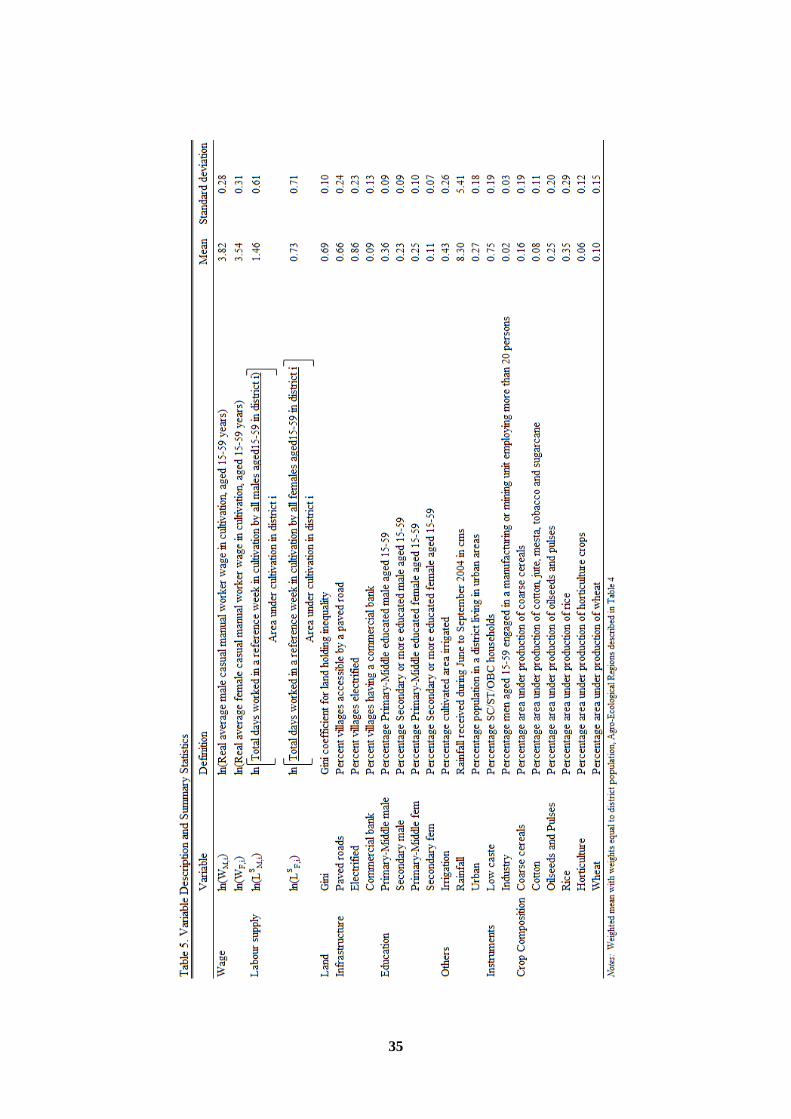
collected from other sources. Table 5 contains a description of the variables, their definitions

and descriptive statistics. Appendix A.1 lists the sources for each variable used.

Aside from the endogenous variables, the control variables are land distribution,

irrigation, rainfall, crop composition, infrastructure (roads, electrification and banking),

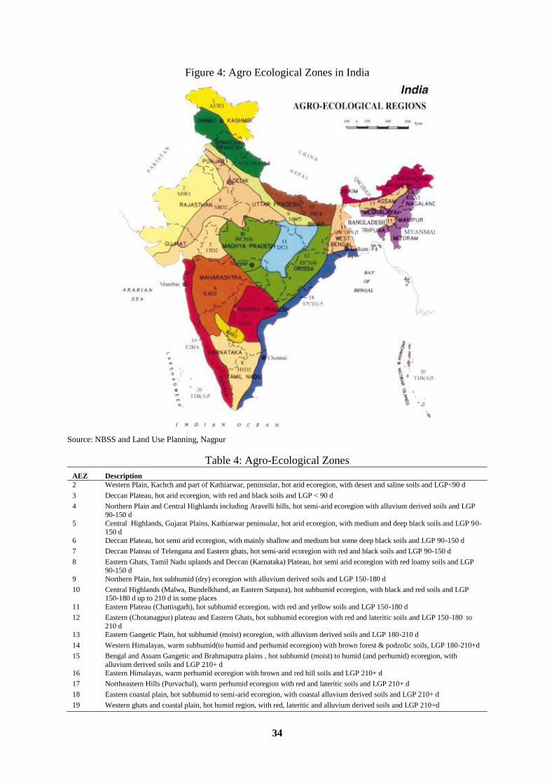
urbanization, education and agro-climatic variables.8 The last set of variables comes from the

classification of the country into 20 agro-ecological zones(AEZ) by the National Bureau of

Soil Survey based on soil, physiography of the area, bioclimatic conditions and length of

growing period which depends on moisture availability in soil. The nature of crops grown in

an area depends on climatic and soil suitability. Table 4 gives a brief description of the

AEZ’s to which the districts in the sample belong. There is no district under AEZ 1 and 20 in

the sample. The independent variables are created by taking the proportion of area of the

district under the particular AEZ. Palmer-Jones and Sen(2003) show that agricultural growth

and poverty reduction in a district depends on whether the district is located in an area where

8 Education and urbanization affect the supply of labor to agriculture. However, this paper does not use them as

instruments because by changing the skill composition of the labor force and also affecting the access to non-

labor inputs, these variables can also affect the demand for agricultural labor.

19

the agro-ecological conditions are favourable to spread of irrigation and agricultural

development. In general AEZ’s having features which are more suitable to agriculture should

positively affect the demand for labor in agriculture.

Our district-level regressions are weighted by district population and the standard

errors are robust and corrected for clustering at state-region level. In some districts, there are

very few wage observations. To avoid the influence of outliers, the districts for which

number of wage observations for either males or females was less than 5 were dropped from

the analyses. Dropping districts where either male or female observations are few in number

results in a data set with equal observations for males and females. However, this could lead

to a biased sample as the districts where female participation in the casual labor market is the

least are most likely to be excluded from the sample. We later see if the results are sensitive

to this type of district selection by estimating male labor demand function for districts in

which number of male wage observations are at least five (ignoring the paucity, if any, in the

number of female observations) and female labor demand function for districts in which

number of female wage observations are at least five (ignoring the paucity, if any, of male

wage observations).

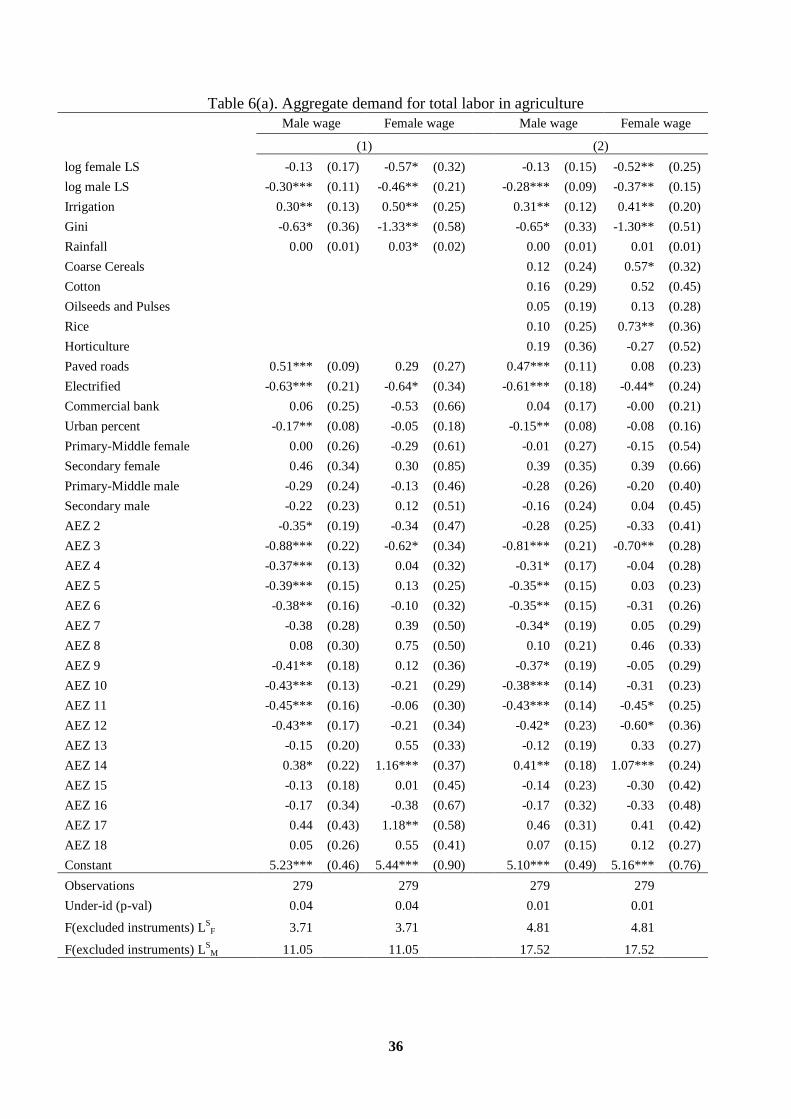
6. Main Findings:

Table 6(a) shows the system two stage least squares estimates of inverse demand

functions for total male and female labor in agriculture. The exclusion restriction implied by

the instrumental variables strategy is that variation in low caste population and access to large

scale non-farm employment affect agricultural wages only through their impact on supply of

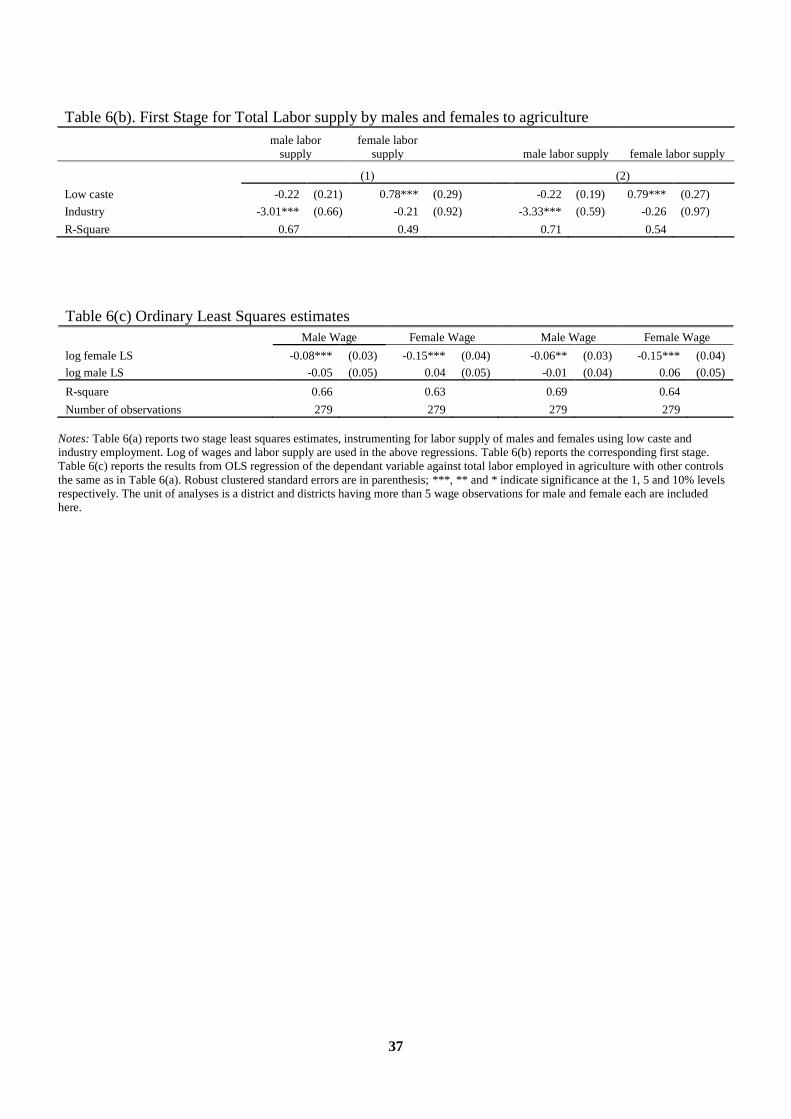
labor to agriculture. Table 6(b) shows the first stage results for the corresponding

specifications in Table 6(a). Table 6(a) considers two specifications. The first specification

includes the controls for land distribution, rainfall, infrastructure, education and agro-

20

ecological regions. The second specification augments the first regression by adding control

variables for crop composition. In the first stage reduced form regressions we find that

greater the proportion of low caste households in a district, greater is female labor supply to

agriculture and that this relation is highly significant in both the specifications. Similarly, a

greater presence of large scale non-farm enterprises in manufacturing and mining sectors

decreases male labor supply to agriculture significantly in both the specifications. The

proportion of low caste households does not affect supply of male labor to agriculture and

presence of large scale non-farm manufacturing and mining enterprises does not affect female

labor supply to agriculture significantly. The F-statistic for the instruments is reported in the

bottom of Table 6(a) and it is highly significant as well. The first stage regressions thus

confirm the causal story about these variables: that status norm govern female labor supply

and that non-farm opportunities are primarily received by men.

The system 2SLS estimates of female and male labor supply are larger in magnitude

than the OLS estimates in Table 6(c), and have the expected negative signs for own effects.

The coefficients of the labor supply variables do not change much between the two

specifications in Table 6(a). The negative signs on cross effects imply that males and females

are substitutes in agriculture.

However, male and female labor are not perfect substitutes. In the system 2SLS

regressions with full set of controls, female labor supply has a significant impact on female

wages with an inverse demand elasticity of – 0.52. However, the impact of female labor

supply on male wages is smaller (around -0.1) and is not significantly different from zero.

Thus, an increase in female labor supply by 10 percent decreases female wages by 5.2

percent and male wages by 1.3 percent and decreases the female to male wage ratio by 4

percent. To test formally that the impact on female wages is greater (in absolute terms) than

the impact on male wages, we estimate the covariance between the two coefficients and carry

21

out a chi-square-test. The chi-square-test rejects the null that the coefficients are equal

against the alternative that the coefficient of female labor supply in the female wage

regression is higher than the coefficient of female labor supply in the male wage regression at

1% level of significance. This is supportive of the Boserup hypothesis that the caste driven

variation in female labor supply leads to variation in the gender wage gap. In particular,

greater female work participation decreases female wages relative to male wages.

In contrast, the effect of male labor supply variation is significant for both male and

female wages. In the second specification with full set of controls, the point estimate of the

inverse demand elasticity is -0.37 for females and -0.28 for males and both are significant.

Although large scale non-farm employment is dominated by men, non-farm labor demand

has favourable effects on female and male wages. The point estimates would imply that a 10

percent decrease in male labor supply increases male wages by 2.8 percent, female wages by

3.7 percent and increases the female to male wage ratio by 1 percent. A chi-square test

however, does not reject the null of equality of the two coefficients in the male and female

inverse demand functions for male labor supply and hence decrease in male labor supply to

agriculture has no significant impact on gender wage differentials in agriculture.

Thus, there is an asymmetry between the effects of gender specific variation in labor

supply on the wages of the opposite gender. Male labor supply matters to female wages but

the effect of female labor supply on male wages is small and insignificant. The theoretical

model posited in section 3 predicts that the elasticity of female wages with respect to male

labor supply relative to the similar cross elasticity for male wages is the product of two ratios:

the ratio of male to female labor employment and the male to female wage ratio. The sample

estimate of male and female labor employment is 5.17 and 2.57 days per week per hectare of

land respectively while the sample estimate for male and female wages is Rs 47.3 and Rs

36.13 per day respectively. This gives an estimate of relative cross price elasticities to be

22

2.63. The baseline results in Table 6(a) with full set of controls give an empirical estimate of

the ratio of cross-price elasticities as 2.84 which is very similar to the theoretical estimate

derived.

The control variables (i.e., other than the labor supply variables) could also have an

effect on the gender wage gap. To ascertain this, a Chi-square test was used to test for the

equality of coefficients of each of the control variables across male and female demand

equations. We find that the null hypothesis of equality of coefficients cannot be rejected for

all except three variables. The null is rejected at the 5% level of significance for rice

cultivation, access to roads and landholding inequality. Areas where more rice is cultivated

have a higher demand for female labor which leads to higher wages for women and translates

into a lower gender wage differential. Many researchers have documented greater demand for

female labor in rice cultivation due to greater efficiency of females in tasks like transplanting

and weeding (Mbiti(2010)) and this result validates their observations. Access to roads on the

other hand only seems to increase demand for male labor resulting in a larger wage

differential between females and males in districts with better access to roads. This possibly

stems from the greater importance of non-farm employment for men. Landholding inequality

measured by the gini coefficient for a district affects demand for both males and females

significantly negatively reflecting the well known feature that large farms use less labor per

unit of land than small farms. However, women are more adversely affected by men

resulting in larger gender wage gaps in districts with higher land inequality. Theoretically, the

effect of landholding inequality on gender wage differentials is ambiguous (Rosenzweig,

1980).

7. Robustness checks

23

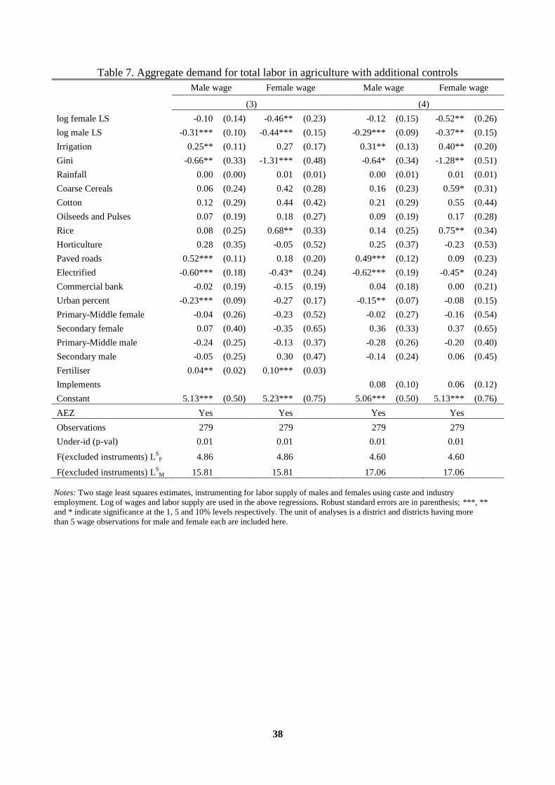
In Table 7 we control for other covariates which could affect demand for labor like

fertiliser usage and tractors and power operated implements per unit land cultivated in a

district. Including fertilisers does not change the impact of female labor supply on male and

female wages and a 10 percent increase in female labor supply increases the gender wage

differential by 3.6 percent. The chi-square test does not reject the equality of male labor

supply coefficients across male and female demand equations but rejects the equality for

female labor supply coefficients. The inclusion of fertilizers does, however, reduce the

coefficient of irrigation in both equations to the point that it becomes insignificant in the

female labor demand equation. This is possibly because of the high positive correlation

between irrigation and fertiliser use. Controlling for implements used per unit land cultivated

does not change any of the principal findings of the base specification. Again, the chi-square

test does not reject the equality of male labor supply coefficients across male and female

demand equations but rejects the equality for female labor supply coefficients.

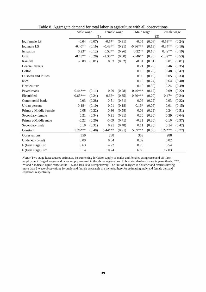
As a second check, we reconsider our sample selection rule. Recall, that we chose

districts for which there were at least five observations for female as well as male wages.

While this ensured equal sample sizes for males and females, it also risked dropping districts

where the female participation in wage work is the least. To ameliorate the possible bias, for

at least, the male labor demand equations, we considered the following alternative. For the

male worker sample, we considered all districts where there at least five observations on male

wages. Similarly, for the female worker sample, we included all districts where there at least

five observations on female wages. This increases the number of districts from 279 in the

matched sample to 359 for males and to 288 for females. Table 8 shows the results from the

estimation of the two specifications on this enlarged sample. In the specification with full set

of controls, an increase in female labor supply decreases the wage ratio while there is no

effect of a change in the male labor supply on the wage ratio. In this respect, the findings of

24

the enlarged sample are no different from what was obtained with the matched sample.

However, the effect of female labor supply in the enlarged sample is greater. A 10% increase

in female labor supply results in a 4.8% decline in the gender wage ratio in the enlarged

sample compared to 4% in the matched sample.

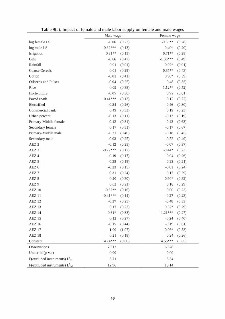
As a third robustness check, we control for differential participation in tasks by males

and females across districts. As noted in section 2, some agricultural tasks are traditionally

deemed as male while others are dominated by women. In section 2, we showed that the raw

correlations between female labor supply and the gender wage gap is robust to the cross-

sectional differences in the gender division of labor. To address this issue formally, we

estimate wage equations at the individual level with explanatory factors for district level male

and female labor supply, other district level controls, individual characteristics (age, age

square, education dummies, and marital status dummies) and dummies for the various

agricultural tasks. The different agricultural tasks are ploughing, sowing, transplanting,

weeding, harvesting and other agricultural activities.

Table 9(a) shows the 2SLS results with the above estimation. The estimates show that

a one percent increase in female labor supply reduces female wage by 0.55% and has no

significant effect on male wage. Male labor supply on the other hand has an identical

negative effect on male and female wage. Thus, the conclusions of the district level

specifications with regard to the impact of male and female labor supply on male and female

wages continue to hold at the individual level with agricultural task controls as well.

8. Explaining the difference in wage gap between northern and southern states of India

While our findings support the Boserup hypothesis, there are other factors as well that

matter to the gender wage gap. So to what extent does the Boserup hypothesis, i.e., the

25

difference in female work participation across northern and southern states in India explain

the observed differences in the gender wage gap?

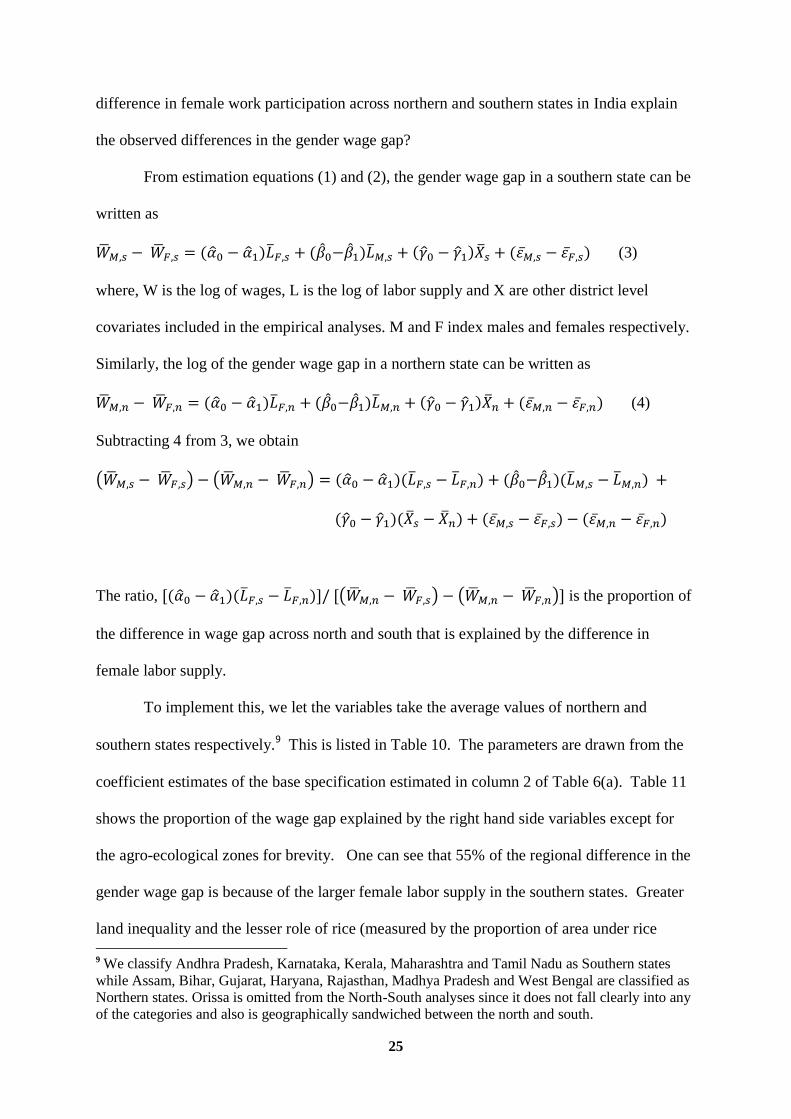
From estimation equations (1) and (2), the gender wage gap in a southern state can be

written as

(3)

where, W is the log of wages, L is the log of labor supply and X are other district level

covariates included in the empirical analyses. M and F index males and females respectively.

Similarly, the log of the gender wage gap in a northern state can be written as

(4)

Subtracting 4 from 3, we obtain

The ratio, is the proportion of

the difference in wage gap across north and south that is explained by the difference in

female labor supply.

To implement this, we let the variables take the average values of northern and

southern states respectively.9 This is listed in Table 10. The parameters are drawn from the

coefficient estimates of the base specification estimated in column 2 of Table 6(a). Table 11

shows the proportion of the wage gap explained by the right hand side variables except for

the agro-ecological zones for brevity. One can see that 55% of the regional difference in the

gender wage gap is because of the larger female labor supply in the southern states. Greater

land inequality and the lesser role of rice (measured by the proportion of area under rice

9 We classify Andhra Pradesh, Karnataka, Kerala, Maharashtra and Tamil Nadu as Southern states

while Assam, Bihar, Gujarat, Haryana, Rajasthan, Madhya Pradesh and West Bengal are classified as

Northern states. Orissa is omitted from the North-South analyses since it does not fall clearly into any

of the categories and also is geographically sandwiched between the north and south.

26

cultivation) are other important and significant factors which lead to a greater wage gap in the

south. On the other hand, greater electrification, lower male supply and the greater

importance of coarse cereal crops (sorghum and millets) should lead to a lower wage gap in

the south but these do not affect the wage gaps significantly in the regressions.

9. Conclusion

Based on the data from the 1950s, the sociologist Ester Boserup noted that the gender wage

differentials in the Southern states of India were greater than in North India. Half a century

later, this pattern has continued to hold. Boserup posited that this could be because of greater

female labor supply in South India where the cultural restrictions on women's participation in

economic activity were less severe than in North India. In this paper we tested this

hypothesis within a neo-classical framework of labor markets.

The paper estimated district level inverse aggregate demand equations for males and

females in agriculture. The exogenous variation in labor supply was identified by spatial

variation in caste composition and non-farm employment of men in large units. The findings

are supportive of the Boserup hypothesis. Female labor supply has sizeable effects on female

wages but not so much on male wages. An immediate implication of the results is the gender

wage gap might be a misleading indicator of the `economic freedom' enjoyed by women.

The gender gap in the labor force participation is important as well.

The paper also found that male labor supply has sizeable effects on male and female

wages. The asymmetry between the effects of female and male labor supply was found to be

consistent with a standard neo-classical model. The strong effect of male labor supply on

female wages is of independent interest. The sectoral mobility of women from the farm to

non-farm sector is much less marked compared to men (Eswaran, et. al, 2009). This could be

because of lower education levels as well societal constraints that limit participation in most

27

non-farm jobs. This raises the concern that the rapid growth of non-farm sector does not

have much to offer to women. Our finding, however, suggests that there is enough

substitutability between men and women in the agricultural production process that a

withdrawal of men from agriculture has positive effects on male and female wages.

The interesting question is whether our findings can be expected to be found across

time. A temporal panel analysis might also be advocated for controlling unobserved

differences across regions. For instance, in the United States, the military mobilization for

World War II led to a sharp rise in women's labor force participation. Using the military

mobilization as an exogenous event, Acemoglu, Autor and Lyle (2004) estimated the effect

of female labor supply increase on female and male wages. In the Indian case, the absence of

such defining exogenous events makes it difficult to study the effect of temporal variation.

The persistence over five decades (from the 1950s to the 2000s) of the spatial patterns in the

gender wage gaps and gender gaps in labor force participation means that panel data analysis

will have little variation to explain. This is much like what was found by Blau and

Kahn(2003) who use a panel of rich and middle-income countries to estimate the impact of

net female labor supply and earnings inequality on the gender wage differential. They find

that the impacts are smaller and often insignificant in the models with country fixed effects.

This is essentially because most of the variation is between countries rather than within-

country. In the absence of major exogenous events that affect work participation, questions

about temporal impacts are difficult to answer.

28

Figure 1: Regional variation in wage ratios, 2004

Source: National sample survey (NSS) 2004, Schedule 10

29

Table1. Female to male wage ratio

State 1983 1993 1999 2004

Assam 86% 81% 78% 90%

Gujarat 88% 98% 89% 90%

West Bengal 93% 88% 89% 88%

Bihar 84% 87% 88% 87%

Haryana 97% 85% 90% 84%

Madhya Pradesh 85% 83% 85% 83%

Punjab 81% 99% 94% 83%

Uttar Pradesh 79% 75% 78% 83%

Rajasthan 65% 75% 80% 81%

Orissa 75% 73% 79% 72%

Karnataka 70% 73% 68% 69%

Andhra Pradesh 66% 72% 67% 65%

Maharashtra 59% 63% 65% 63%

Kerala 65% 70% 63% 59%

Tamil Nadu 55% 57% 58% 54%

All India 69% 72% 72% 70%

Source: NSS Schedule 10, 1983, 1993, 1999, 2004

30

Figure 2

Figure 2(a) Figure 2(b)

Figure 2(c) Figure 2(d)

Figure 2(e) Figure 2(f)

2(a) Sex ratio

2(b) Percent women having body mass index below 18.5

2(c) Percent women who have experienced physical/sexual violence

2(d) Percent women who make the decision to visit family/relatives

2(e) Percent women who make the decision regarding major household purchases

2(f) Percent women allowed to the market, to the health facility, and to places outside the village alone Population weighted regression lines are fitted to the above plots

Source: NSS 2004 Schedule 10, National Family and Health Survey (NFHS) 2005-06

PunjabHaryana

Raj

UP

Bihar

Assam

WBOrissa

MP

Guj

Maha

AP

Kar

KeralaTN

900

950

100

01

05

01

10

0

se

xra

tio

.5 .6 .7 .8 .9Wage ratio

Fitted values

Punjab

Haryana

Raj UP

Bihar

Assam

WB

Orissa

MPGujMaha

AP

Kar

Kerala

TN

20

30

40

50

bm

i

.5 .6 .7 .8 .9Wage ratio

Fitted values

Punjab

Haryana

Raj

UP

Bihar

AssamWB

Orissa

MP

Guj

Maha

AP

Kar

Kerala

TN

20

30

40

50

60

Ph

ysic

al or

sexu

al vio

len

ce

.5 .6 .7 .8 .9Wage ratio

Fitted values

Punjab

Haryana

Raj

UP

BiharAssam

WB

OrissaMP

Guj

Maha

AP

Kar

Kerala

TN

51

01

52

0

Fam

ily v

isit b

y w

om

an

.5 .6 .7 .8 .9Wage ratio

Fitted values

Punjab

HaryanaRajUP

Bihar

AssamWB

Orissa

MP

GujMaha

APKar

Kerala

TN

51

01

52

0

Ma

jor

purc

hase

s b

y w

om

an

.5 .6 .7 .8 .9Wage ratio

Fitted values

Punjab Haryana

Raj

UP

Bihar

Assam

WB

Orissa

MP

Guj

Maha

AP

Kar

Kerala

TN

20

30

40

50

Allo

we

d a

lon

e

.5 .6 .7 .8 .9Wage ratio

Fitted values

31

Figure 3: Female labor supply and the gender wage ratio

Notes- Labor supply is measured as total days worked in a reference week per unit land under cultivation,

- Population weighted regression lines are fitted to the above plots; Source: NSS 2004 Schedule 10

Figure 4(a): Gender-segregation and the gender wage ratio

Notes- Labor supply is measured as total days worked in a reference week per unit land under cultivation,

- Population weighted regression lines are fitted to the above plots; Source: NSS 2004 Schedule 10

PunjabHaryana

Raj

UP

Bihar

Assam

WB

Orissa

MP

Guj

Maha

AP

Kar

Kerala

TN

.5.6

.7.8

.9

Wag

e r

atio

0 1 2 3 4Female labour supply

Punjab HaryanaRajUP

BiharAssamWB

Orissa

MP

Guj

Maha

AP

Kar

Kerala

TN

.5.6

.7.8

.9

Wag

e r

atio

.1 .2 .3 .4 .5 .6Gender segregation

Fitted values

32

Figure 4(b): Female labor supply and the re-weighted gender wage ratio

Notes- Labor supply is measured as total days worked in a reference week per unit land under cultivation,

- Population weighted regression lines are fitted to the above plots; Source: NSS 2004 Schedule 10

Figure 5: Labor supply ratio and the gender wage ratio

Notes- Labor supply is measured as total days worked in a reference week per unit land under cultivation,

- Labor supply ratio is =Female labor supply/Male labor supply

- Population weighted regression lines are fitted to the above plots; Source: NSS 2004 Schedule 10

Punjab

Haryana

Raj

UP

Bihar

Assam

WB

Orissa

MP

Guj

MahaAP

Kar

Kerala

TN

.5.6

.7.8

.9

Wag

e r

atio

re

we

ighte

d

0 1 2 3 4Female labour supply

Punjab Haryana

Raj

UP

Bihar

Assam

WB

Orissa

MP

Guj

Maha

AP

Kar

Kerala

TN

.5.6

.7.8

.9

Wag

e r

atio

0 .2 .4 .6 .8 1Labour supply ratio

Fitted values

33

Table 2: Task wise allocation of workers in agriculture

Task Male Female

Ploughing 95% 5%

Sowing 67% 33%

Transplanting 55% 45%

Weeding 48% 52%

Harvesting 63% 37%

Other cultivation activities 73% 27%

All activities 67% 33%

Source: NSS 2004 Schedule 10

Table 3: Sectoral distribution of off-farm employment

Industry

Percentage in units with 20 or

more workers

Percentage in units with 9 or less

workers

(1) (2)

Agriculture and allied activities 1% 7%

Fishing 0% 1%

Mining 7% 1%

Manufacturing 44% 20%

Construction 11% 17%

Trade and hotels 3% 28%

Transport 9% 12%

Finance and real estate 3% 2%

Public administration 22% 11%

Domestic services 0% 1%

Notes: The above figures are calculated from the usual status activity status of respondents in NSS 2004 Schedule 10 for

men aged 15-59

34

Figure 4: Agro Ecological Zones in India

Source: NBSS and Land Use Planning, Nagpur

Table 4: Agro-Ecological Zones

AEZ Description

2 Western Plain, Kachch and part of Kathiarwar, peninsular, hot arid ecoregion, with desert and saline soils and LGP<90 d

3 Deccan Plateau, hot arid ecoregion, with red and black soils and LGP < 90 d

4 Northern Plain and Central Highlands including Aravelli hills, hot semi-arid ecoregion with alluvium derived soils and LGP

90-150 d

5 Central Highlands, Gujarat Plains, Kathiarwar peninsular, hot arid ecoregion, with medium and deep black soils and LGP 90-

150 d

6 Deccan Plateau, hot semi arid ecoregion, with mainly shallow and medium but some deep black soils and LGP 90-150 d

7 Deccan Plateau of Telengana and Eastern ghats, hot semi-arid ecoregion with red and black soils and LGP 90-150 d

8 Eastern Ghats, Tamil Nadu uplands and Deccan (Karnataka) Plateau, hot semi arid ecoregion with red loamy soils and LGP 90-150 d

9 Northern Plain, hot subhumid (dry) ecoregion with alluvium derived soils and LGP 150-180 d

10 Central Highlands (Malwa, Bundelkhand, an Eastern Satpura), hot subhumid ecoregion, with black and red soils and LGP

150-180 d up to 210 d in some places

11 Eastern Plateau (Chattisgarh), hot subhumid ecoregion, with red and yellow soils and LGP 150-180 d

12 Eastern (Chotanagpur) plateau and Eastern Ghats, hot subhumid ecoregion with red and lateritic soils and LGP 150-180 to

210 d 13 Eastern Gangetic Plain, hot subhumid (moist) ecoregion, with alluvium derived soils and LGP 180-210 d

14 Western Himalayas, warm subhumid(to humid and perhumid ecoregion) with brown forest & podzolic soils, LGP 180-210+d

15 Bengal and Assam Gangetic and Brahmaputra plains , hot subhumid (moist) to humid (and perhumid) ecoregion, with

alluvium derived soils and LGP 210+ d

16 Eastern Himalayas, warm perhumid ecoregion with brown and red hill soils and LGP 210+ d

17 Northeastern Hills (Purvachal), warm perhumid ecoregion with red and lateritic soils and LGP 210+ d

18 Eastern coastal plain, hot subhumid to semi-arid ecoregion, with coastal alluvium derived soils and LGP 210+ d

19 Western ghats and coastal plain, hot humid region, with red, lateritic and alluvium derived soils and LGP 210+d

35

36

Table 6(a). Aggregate demand for total labor in agriculture

Male wage Female wage

Male wage Female wage

(1) (2)

log female LS -0.13 (0.17) -0.57* (0.32)

-0.13 (0.15) -0.52** (0.25)

log male LS -0.30*** (0.11) -0.46** (0.21)

-0.28*** (0.09) -0.37** (0.15)

Irrigation 0.30** (0.13) 0.50** (0.25)

0.31** (0.12) 0.41** (0.20)

Gini -0.63* (0.36) -1.33** (0.58)

-0.65* (0.33) -1.30** (0.51)

Rainfall 0.00 (0.01) 0.03* (0.02)

0.00 (0.01) 0.01 (0.01)

Coarse Cereals

0.12 (0.24) 0.57* (0.32)

Cotton

0.16 (0.29) 0.52 (0.45)

Oilseeds and Pulses

0.05 (0.19) 0.13 (0.28)

Rice

0.10 (0.25) 0.73** (0.36)

Horticulture

0.19 (0.36) -0.27 (0.52)

Paved roads 0.51*** (0.09) 0.29 (0.27)

0.47*** (0.11) 0.08 (0.23)

Electrified -0.63*** (0.21) -0.64* (0.34)

-0.61*** (0.18) -0.44* (0.24)

Commercial bank 0.06 (0.25) -0.53 (0.66)

0.04 (0.17) -0.00 (0.21)

Urban percent -0.17** (0.08) -0.05 (0.18)

-0.15** (0.08) -0.08 (0.16)

Primary-Middle female 0.00 (0.26) -0.29 (0.61)

-0.01 (0.27) -0.15 (0.54)

Secondary female 0.46 (0.34) 0.30 (0.85)

0.39 (0.35) 0.39 (0.66)

Primary-Middle male -0.29 (0.24) -0.13 (0.46)

-0.28 (0.26) -0.20 (0.40)

Secondary male -0.22 (0.23) 0.12 (0.51)

-0.16 (0.24) 0.04 (0.45)

AEZ 2 -0.35* (0.19) -0.34 (0.47)

-0.28 (0.25) -0.33 (0.41)

AEZ 3 -0.88*** (0.22) -0.62* (0.34)

-0.81*** (0.21) -0.70** (0.28)

AEZ 4 -0.37*** (0.13) 0.04 (0.32)

-0.31* (0.17) -0.04 (0.28)

AEZ 5 -0.39*** (0.15) 0.13 (0.25)

-0.35** (0.15) 0.03 (0.23)

AEZ 6 -0.38** (0.16) -0.10 (0.32)

-0.35** (0.15) -0.31 (0.26)

AEZ 7 -0.38 (0.28) 0.39 (0.50)

-0.34* (0.19) 0.05 (0.29)

AEZ 8 0.08 (0.30) 0.75 (0.50)

0.10 (0.21) 0.46 (0.33)

AEZ 9 -0.41** (0.18) 0.12 (0.36)

-0.37* (0.19) -0.05 (0.29)

AEZ 10 -0.43*** (0.13) -0.21 (0.29)

-0.38*** (0.14) -0.31 (0.23)

AEZ 11 -0.45*** (0.16) -0.06 (0.30)

-0.43*** (0.14) -0.45* (0.25)

AEZ 12 -0.43** (0.17) -0.21 (0.34)

-0.42* (0.23) -0.60* (0.36)

AEZ 13 -0.15 (0.20) 0.55 (0.33)

-0.12 (0.19) 0.33 (0.27)

AEZ 14 0.38* (0.22) 1.16*** (0.37)

0.41** (0.18) 1.07*** (0.24)

AEZ 15 -0.13 (0.18) 0.01 (0.45)

-0.14 (0.23) -0.30 (0.42)

AEZ 16 -0.17 (0.34) -0.38 (0.67)

-0.17 (0.32) -0.33 (0.48)

AEZ 17 0.44 (0.43) 1.18** (0.58)

0.46 (0.31) 0.41 (0.42)

AEZ 18 0.05 (0.26) 0.55 (0.41)

0.07 (0.15) 0.12 (0.27)

Constant 5.23*** (0.46) 5.44*** (0.90) 5.10*** (0.49) 5.16*** (0.76)

Observations 279

279

279

279

Under-id (p-val) 0.04

0.04

0.01

0.01

F(excluded instruments) L

SF 3.71

3.71

4.81

4.81

F(excluded instruments) L

SM 11.05 11.05 17.52 17.52

37

Table 6(b). First Stage for Total Labor supply by males and females to agriculture

male labor

supply

female labor

supply male labor supply female labor supply

(1) (2)

Low caste -0.22 (0.21) 0.78*** (0.29)

-0.22 (0.19) 0.79*** (0.27)

Industry -3.01*** (0.66) -0.21 (0.92)

-3.33*** (0.59) -0.26 (0.97)

R-Square 0.67 0.49 0.71 0.54

Table 6(c) Ordinary Least Squares estimates

Male Wage Female Wage

Male Wage Female Wage

log female LS -0.08*** (0.03) -0.15*** (0.04)

-0.06** (0.03) -0.15*** (0.04)

log male LS -0.05 (0.05) 0.04 (0.05)

-0.01 (0.04) 0.06 (0.05)

R-square 0.66 0.63 0.69 0.64

Number of observations 279 279 279 279

Notes: Table 6(a) reports two stage least squares estimates, instrumenting for labor supply of males and females using low caste and

industry employment. Log of wages and labor supply are used in the above regressions. Table 6(b) reports the corresponding first stage.

Table 6(c) reports the results from OLS regression of the dependant variable against total labor employed in agriculture with other controls

the same as in Table 6(a). Robust clustered standard errors are in parenthesis; ***, ** and * indicate significance at the 1, 5 and 10% levels

respectively. The unit of analyses is a district and districts having more than 5 wage observations for male and female each are included

here.

38

Table 7. Aggregate demand for total labor in agriculture with additional controls

Male wage Female wage

Male wage Female wage

(3) (4)

log female LS -0.10 (0.14) -0.46** (0.23)

-0.12 (0.15) -0.52** (0.26)

log male LS -0.31*** (0.10) -0.44*** (0.15)

-0.29*** (0.09) -0.37** (0.15)

Irrigation 0.25** (0.11) 0.27 (0.17)

0.31** (0.13) 0.40** (0.20)

Gini -0.66** (0.33) -1.31*** (0.48)

-0.64* (0.34) -1.28** (0.51)

Rainfall 0.00 (0.00) 0.01 (0.01)

0.00 (0.01) 0.01 (0.01)

Coarse Cereals 0.06 (0.24) 0.42 (0.28)

0.16 (0.23) 0.59* (0.31)

Cotton 0.12 (0.29) 0.44 (0.42)

0.21 (0.29) 0.55 (0.44)

Oilseeds and Pulses 0.07 (0.19) 0.18 (0.27)

0.09 (0.19) 0.17 (0.28)

Rice 0.08 (0.25) 0.68** (0.33)

0.14 (0.25) 0.75** (0.34)

Horticulture 0.28 (0.35) -0.05 (0.52)

0.25 (0.37) -0.23 (0.53)

Paved roads 0.52*** (0.11) 0.18 (0.20)

0.49*** (0.12) 0.09 (0.23)

Electrified -0.60*** (0.18) -0.43* (0.24)

-0.62*** (0.19) -0.45* (0.24)

Commercial bank -0.02 (0.19) -0.15 (0.19)

0.04 (0.18) 0.00 (0.21)

Urban percent -0.23*** (0.09) -0.27 (0.17)

-0.15** (0.07) -0.08 (0.15)

Primary-Middle female -0.04 (0.26) -0.23 (0.52)

-0.02 (0.27) -0.16 (0.54)

Secondary female 0.07 (0.40) -0.35 (0.65)

0.36 (0.33) 0.37 (0.65)

Primary-Middle male -0.24 (0.25) -0.13 (0.37)

-0.28 (0.26) -0.20 (0.40)

Secondary male -0.05 (0.25) 0.30 (0.47)

-0.14 (0.24) 0.06 (0.45)

Fertiliser 0.04** (0.02) 0.10*** (0.03)

Implements

0.08 (0.10) 0.06 (0.12)

Constant 5.13*** (0.50) 5.23*** (0.75) 5.06*** (0.50) 5.13*** (0.76)

AEZ Yes Yes Yes Yes

Observations 279

279

279

279

Under-id (p-val) 0.01

0.01

0.01

0.01

F(excluded instruments) L

SF 4.86

4.86

4.60

4.60

F(excluded instruments) L

SM 15.81 15.81 17.06 17.06

Notes: Two stage least squares estimates, instrumenting for labor supply of males and females using caste and industry

employment. Log of wages and labor supply are used in the above regressions. Robust standard errors are in parenthesis; ***, **

and * indicate significance at the 1, 5 and 10% levels respectively. The unit of analyses is a district and districts having more

than 5 wage observations for male and female each are included here.

39

Table 8. Aggregate demand for total labor in agriculture with all observations

Male wage Female wage Male wage Female wage

(1) (2)

log female LS -0.04 (0.07) -0.57* (0.31) -0.05 (0.06) -0.53** (0.24)

log male LS -0.40** (0.19) -0.43** (0.21) -0.36*** (0.13) -0.34** (0.16)

Irrigation 0.23* (0.12) 0.52** (0.26) 0.22** (0.10) 0.42** (0.19)

Gini -0.45** (0.20) -1.36** (0.60) -0.46** (0.20) -1.32** (0.53)

Rainfall -0.00 (0.01) 0.03 (0.02) -0.01 (0.01) 0.01 (0.01)

Coarse Cereals

0.21 (0.23) 0.46 (0.35)

Cotton

0.18 (0.26) 0.48 (0.47)

Oilseeds and Pulses

0.05 (0.19) 0.05 (0.33)

Rice

0.19 (0.24) 0.64 (0.40)

Horticulture

0.10 (0.39) -0.24 (0.49)

Paved roads 0.44*** (0.11) 0.29 (0.28) 0.40*** (0.12) 0.09 (0.22)

Electrified -0.65*** (0.24) -0.66* (0.35) -0.60*** (0.20) -0.47* (0.24)

Commercial bank -0.03 (0.28) -0.51 (0.61) 0.06 (0.22) -0.03 (0.22)

Urban percent -0.18* (0.10) 0.01 (0.18) -0.16* (0.09) -0.01 (0.15)

Primary-Middle female 0.08 (0.22) -0.36 (0.58) 0.08 (0.22) -0.24 (0.51)

Secondary female 0.21 (0.34) 0.21 (0.81) 0.20 (0.30) 0.29 (0.64)

Primary-Middle male -0.22 (0.20) -0.09 (0.41) -0.21 (0.20) -0.16 (0.37)

Secondary male 0.10 (0.31) 0.21 (0.48) 0.11 (0.26) 0.14 (0.42)

Constant 5.26*** (0.48) 5.44*** (0.91) 5.09*** (0.50) 5.22*** (0.77)

Observations 359

288

359

288

Under-id (p-val) 0.09

0.04

0.02

0.02

F (First stage) lsf 8.63

4.22

8.76

5.54

F (First stage) lsm 3.14 10.74 6.69 17.03

Notes: Two stage least squares estimates, instrumenting for labor supply of males and females using caste and off-farm

employment. Log of wages and labor supply are used in the above regressions. Robust standard errors are in parenthesis; ***,

** and * indicate significance at the 1, 5 and 10% levels respectively. The unit of analyses is a district and districts having

more than 5 wage observations for male and female separately are included here for estimating male and female demand

equations respectively.

40

Table 9(a). Impact of female and male labor supply on female and male wages

Male wage Female wage

log female LS -0.06 (0.23) -0.55** (0.28)

log male LS -0.39*** (0.13) -0.40* (0.20)

Irrigation 0.31** (0.15) 0.71** (0.28)

Gini -0.66 (0.47) -1.36*** (0.49)

Rainfall 0.01 (0.01) 0.02* (0.01)

Coarse Cereals 0.01 (0.29) 0.85** (0.43)

Cotton -0.01 (0.41) 0.98* (0.59)

Oilseeds and Pulses -0.04 (0.25) 0.48 (0.35)

Rice 0.09 (0.38) 1.12** (0.52)

Horticulture -0.05 (0.36) 0.92 (0.61)

Paved roads 0.41*** (0.13) 0.12 (0.22)

Electrified -0.34 (0.26) -0.46 (0.30)

Commercial bank 0.49 (0.33) 0.19 (0.25)

Urban percent -0.13 (0.11) -0.13 (0.19)

Primary-Middle female -0.12 (0.31) -0.42 (0.63)

Secondary female 0.17 (0.51) -0.17 (0.67)

Primary-Middle male -0.21 (0.40) -0.18 (0.45)

Secondary male -0.03 (0.25) 0.52 (0.49)

AEZ 2 -0.12 (0.25) -0.07 (0.37)

AEZ 3 -0.72*** (0.17) -0.44* (0.23)

AEZ 4 -0.19 (0.17) 0.04 (0.26)

AEZ 5 -0.28 (0.19) 0.22 (0.21)

AEZ 6 -0.23 (0.15) -0.01 (0.24)

AEZ 7 -0.31 (0.24) 0.17 (0.29)

AEZ 8 0.20 (0.30) 0.60* (0.32)

AEZ 9 0.02 (0.21) 0.18 (0.29)

AEZ 10 -0.32** (0.16) 0.00 (0.23)

AEZ 11 -0.41*** (0.14) -0.27 (0.23)

AEZ 12 -0.27 (0.25) -0.48 (0.33)

AEZ 13 0.17 (0.22) 0.52* (0.29)

AEZ 14 0.61* (0.33) 1.21*** (0.27)

AEZ 15 0.12 (0.27) -0.24 (0.40)

AEZ 16 -0.15 (0.44) -0.19 (0.61)

AEZ 17 1.00 (1.07) 0.96* (0.53)

AEZ 18 0.21 (0.18) 0.24 (0.26)

Constant 4.74*** (0.60) 4.55*** (0.65)

Observations 7,812

6,378

Under-id (p-val) 0.00

0.00

F(excluded instruments) L

SF 3.71

5.34

F(excluded instruments) L

SM 12.96 13.14

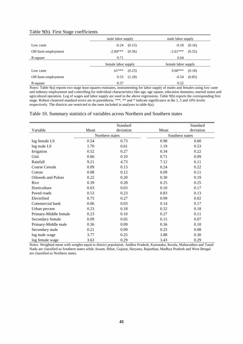
41

Table 9(b). First Stage coefficients

male labor supply male labor supply

Low caste -0.24 (0.15) -0.18 (0.16)

Off-farm employment -2.84*** (0.56) -2.61*** (0.55)

R-square 0.71

0.64

female labor supply female labor supply

Low caste .61*** (0.23) 0.60*** (0.18)

Off-farm employment 0.53 (1.18) -0.54 (0.85)

R-square 0.57 0.52

Notes: Table 9(a) reports two stage least squares estimates, instrumenting for labor supply of males and females using low caste

and industry employment and controlling for individual characteristics like age, age square, education dummies, marital status and

agricultural operation. Log of wages and labor supply are used in the above regressions. Table 9(b) reports the corresponding first

stage. Robust clustered standard errors are in parenthesis; ***, ** and * indicate significance at the 1, 5 and 10% levels

respectively. The districts are restricted to the ones included in analyses in table 6(a).

Table 10. Summary statistics of variables across Northern and Southern states

Variable Mean

Standard

deviation Mean

Standard

deviation

Northern states Southern states

log female LS 0.54 0.73

0.98 0.60

log male LS 1.70 0.61

1.19 0.53

Irrigation 0.52 0.27

0.34 0.22

Gini 0.66 0.10

0.71 0.09

Rainfall 9.21 4.73

7.12 6.11

Coarse Cereals 0.09 0.13

0.24 0.22

Cotton 0.08 0.12

0.09 0.11

Oilseeds and Pulses 0.22 0.20

0.30 0.19

Rice 0.39 0.28

0.25 0.25

Horticulture 0.03 0.03

0.10 0.17

Paved roads 0.53 0.23

0.83 0.13

Electrified 0.75 0.27

0.99 0.02

Commercial bank 0.06 0.03

0.14 0.17

Urban percent 0.23 0.18

0.32 0.18

Primary-Middle female 0.23 0.10

0.27 0.11

Secondary female 0.09 0.05

0.15 0.07

Primary-Middle male 0.36 0.09

0.36 0.10

Secondary male 0.21 0.09

0.25 0.08

log male wage 3.77 0.25

3.88 0.30

log female wage 3.63 0.29 3.43 0.29 Notes: Weighted mean with weights equal to district population. Andhra Pradesh, Karnataka, Kerala, Maharashtra and Tamil

Nadu are classified as Southern states while Assam, Bihar, Gujarat, Haryana, Rajasthan, Madhya Pradesh and West Bengal

are classified as Northern states.

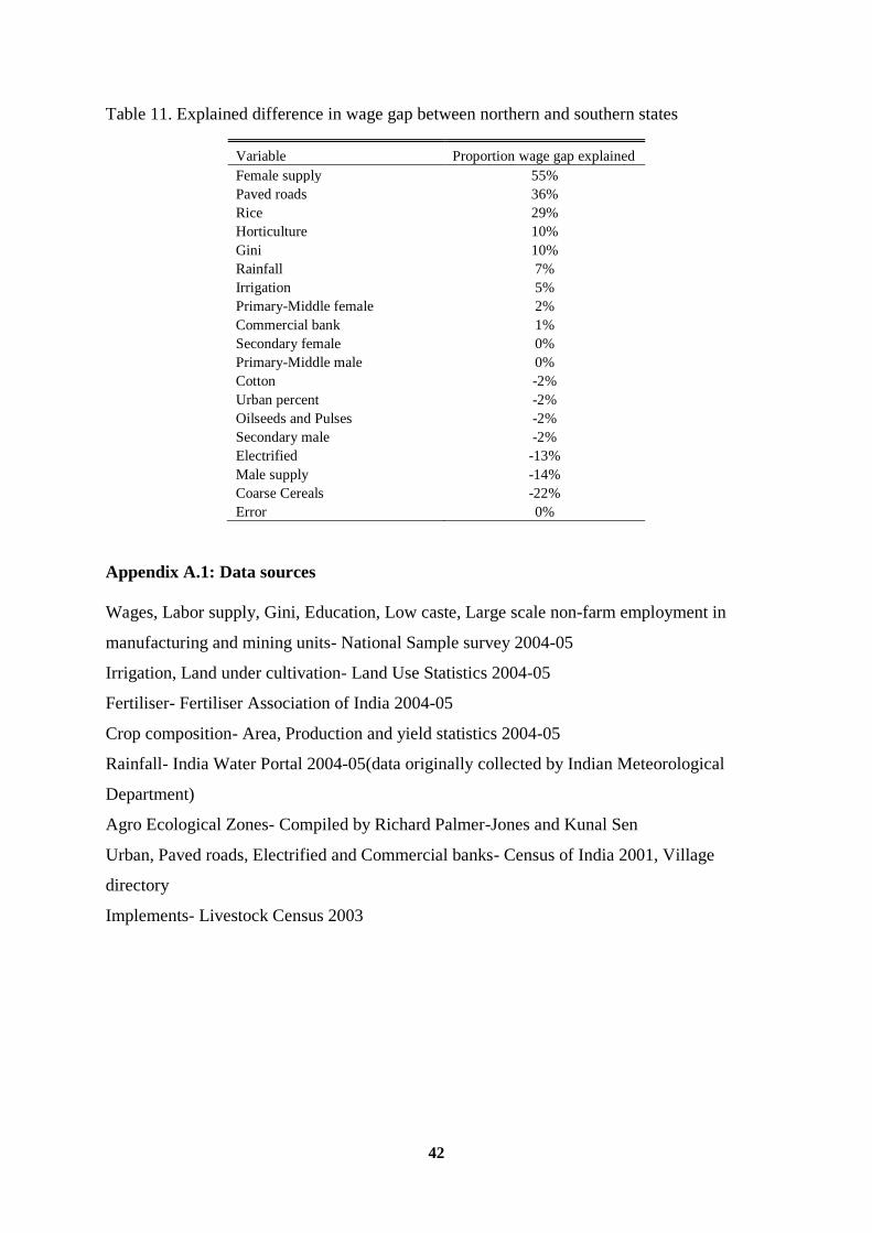
42

Table 11. Explained difference in wage gap between northern and southern states

Variable Proportion wage gap explained

Female supply 55%

Paved roads 36%

Rice 29%

Horticulture 10%

Gini 10%

Rainfall 7%

Irrigation 5%

Primary-Middle female 2%

Commercial bank 1%

Secondary female 0%

Primary-Middle male 0%

Cotton -2%

Urban percent -2%

Oilseeds and Pulses -2%

Secondary male -2%

Electrified -13%

Male supply -14%

Coarse Cereals -22%

Error 0%

Appendix A.1: Data sources

Wages, Labor supply, Gini, Education, Low caste, Large scale non-farm employment in

manufacturing and mining units- National Sample survey 2004-05

Irrigation, Land under cultivation- Land Use Statistics 2004-05

Fertiliser- Fertiliser Association of India 2004-05

Crop composition- Area, Production and yield statistics 2004-05

Rainfall- India Water Portal 2004-05(data originally collected by Indian Meteorological

Department)

Agro Ecological Zones- Compiled by Richard Palmer-Jones and Kunal Sen

Urban, Paved roads, Electrified and Commercial banks- Census of India 2001, Village

directory

Implements- Livestock Census 2003

43

References

Acemoglu, Daron, David H. Autor, and David Lyle (2004). “Women, War, and Wages: The

Effect of Female Labor Supply on the Wage Structure at Mid-Century.” Journal of Political

Economy, 112(3), pp. 497-551.

Aggarwal, Bina (1986), “Women, Poverty and Agricultural Growth in India”, The Journal of

Peasant Studies, Vol 13, No 4, July 1986.

Aggarwal, Bina (1994), “A Field of One’s Own: Gender and Land rights in South Asia”,

Cambridge: Cambridge University Press

Anderson, S., (2011), “Caste as an Impediment to Trade”, American Economic Journal:

Applied Economics, Vol. 3, No. 1: Pages 239-263

Banerjee, A. and Rohini Somanathan (2007), “The political economy of public goods: Some

evidence from India”, Journal of Development Economics, 82, pp 287–314

Bardhan, K. (1984). “Work Patterns and Social Differentiation: Rural Women of West

Bengal”, in H.P. Binswanger and M. R. Rosenzweig (eds), Contractual Arrangements,

Employment and Wages in Rural Labor Markets in Asia. Yale University Press, New Haven,

pp.184-208

Bardhan, P. (1979). “Labor supply functions in a poor agrarian economy”, American

Economic Review, Vol. 69, pp. 73–83.

Bardhan, P. (1984). “Determinants of supply and demand for labor in a poor agrarian

economy: an analysis of household survey data from rural West Bengal”, in Binswanger

H. P. and Rosenzweig M. R. (eds), Contractual Arrangements, Employment and Wages in

Rural Labor Markets in Asia. Yale University Press, New Haven.

Basu, Alaka M. (1992), Culture, the Status of Women, and Demographic Behaviour:

Illustrated with the Case of India. Oxford: Clarendon Press.

Beteille, Andre (1969), Caste, Class and Power: Changing Patterns of Stratification in a

Tanjore Village. University of California Press.

Bhalla, G.S. and G. Singh, 2001, Indian agriculture: Four Decades of Development, New

Delhi: Sage

Binswanger, Hans P., Khandker, S., and M. R. Rosenzweig (1993), “How infrastructure and

financial institutions affect agricultural output and investment in India”, Journal of

Development Economics Volume 41, Issue 2, Pages 337-366

Blau and Kahn(2003). “Understanding International Differences in the Gender Pay Gap”,

Journal of Labor Economics, Vol. 21, No. 1, pp. 106-144

Boserup, E. (1970). Women's role in economic development. New York: St. Martin'

Burton, M. L., & White, D. R. (1984), “Sexual division of labor in agriculture”, American

Anthropologist, 86, 568–583

44

Chakravorty , S. and S.V. Lall (2005) “Industrial Location and Spatial Inequality: Theory

and Evidence from India”, Review of Development Economics, 9(1), 47–68

Chavan, P. and Bedamatta, R. (2006) Trends in agricultural wages in India: 1964–65 to

1999–2000. Economic and Political Weekly, 41(38), pp. 4041–4052

Chen, Martha (1995), “A Matter of Survival: Women”s Right to Employment in India and

Bangladesh” in Martha C. Nussbaum and Jonathan Glover (eds), Women, culture and

development: a study of human capabilities. Oxford: Oxford University Press, pp. 37-59

Chen, Martha (1989), “Women’s Work in Indian Agriculture by Agro-Ecologic Zones:

Meeting Needs of Landless and Land-Poor Women”, Economic and Political Weekly, Vol.

24, No. 43, pp. WS79- WS89.

Das, M.B. (2006), “Do Traditional Axes of Exclusion Affect Labor Market Outcomes in

India?” Social Development Papers, South Asia Series, Paper no. 97

Das, M. B., & Dutta, P. V. (2008), “Does caste matter for wages in the Indian labor market?”

paper presented at the third IZA/World Bank conference on employment and development,

Rabat Morocco May 2008

Dyson, Tim and Mick Moore (1983) “On kinship structure, female autonomy, and

demographic behavior in India,” Population and Development Review 9(1): 35–60.

Eswaran, Mukesh, Ramaswami, Bharat and Wilima Wadhwa (2012), “Status, Caste, and the

Time Allocation of Women in Rural India”, forthcoming in Economic Development and

Cultural Change.

Eswaran, M., A. Kotwal, B. Ramaswami and W. Wadhwa. 2009. “Sectoral Labor Flows and

Agricultural Wages in India, 1982-2004: Has Growth Trickled Down?” Economic and

Political Weekly, 44(2): 46–55.

Evenson, R. E. and Binswanger, H. P. (1984). “Estimating labor demand functions for

Indian agriculture”, in Binswanger H. P. and Rosenzweig M. R. (eds), Contractual

Arrangements, Employment and Wages in Rural Labor Markets in Asia, Yale University

Press, New Haven.

Food and Agriculture Organisation (2010), “Gender dimensions of agricultural and rural

employment: Differentiated pathways out of poverty Status, trends and gaps.”

Food and Agriculture Organisation (2011), “Women in agriculture: Closing the gender gap

for development.”

Foster, A. and Rosenzweig, M., (2003), “Agricultural Productivity Growth, Rural Economic

Diversity, and Economic Reforms: India, 1970-2000”, Working Paper.

Gajbhiye, K.S. and C. Mandal “Agro-Ecological Zones, their Soil Resource and Cropping

Systems”, National Bureau of Soil Survey and Land Use Planning, Nagpur

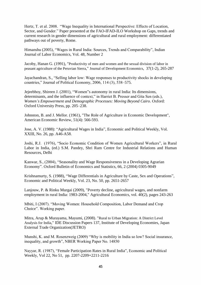
45

Hertz, T. et al. 2008. “Wage Inequality in International Perspective: Effects of Location,

Sector, and Gender.” Paper presented at the FAO-IFAD-ILO Workshop on Gaps, trends and

current research in gender dimensions of agricultural and rural employment: differentiated

pathways out of poverty, Rome.

Himanshu (2005), “Wages in Rural India: Sources, Trends and Comparability”, Indian

Journal of Labor Economics, Vol. 48, Number 2

Jacoby, Hanan G. (1991), "Productivity of men and women and the sexual division of labor in

peasant agriculture of the Peruvian Sierra," Journal of Development Economics, 37(1-2), 265-287

Jayachandran, S., “Selling labor low: Wage responses to productivity shocks in developing

countries,” Journal of Political Economy, 2006, 114 (3), 538–575.

Jejeebhoy, Shireen J. (2001), “Women”s autonomy in rural India: Its dimensions,

determinants, and the influence of context,” in Harriet B. Presser and Gita Sen (eds.),

Women’s Empowerment and Demographic Processes: Moving Beyond Cairo. Oxford:

Oxford University Press, pp. 205–238.

Johnston, B. and J. Mellor. (1961), "The Role of Agriculture in Economic Development",

American Economic Review, 51(4): 566-593.

Jose, A. V. (1988): “Agricultural Wages in India”, Economic and Political Weekly, Vol.

XXIII, No. 26, pp. A46-A58.

Joshi, R.J. (1976), “Socio Economic Condition of Women Agricultural Workers”, in Rural

Labor in India, (ed.) S.M. Pandey, Shri Ram Centre for Industrial Relations and Human

Resources, Delhi

Kanwar, S., (2004), “Seasonality and Wage Responsiveness in a Developing Agrarian

Economy”. Oxford Bulletin of Economics and Statistics, 66, 2 (2004) 0305-9049

Krishnamurty, S. (1988), “Wage Differentials in Agriculture by Caste, Sex and Operations”,

Economic and Political Weekly, Vol. 23, No. 50, pp. 2651-2657

Lanjouw, P. & Rinku Murgai (2009), "Poverty decline, agricultural wages, and nonfarm

employment in rural India: 1983-2004," Agricultural Economics, vol. 40(2), pages 243-263

Mbiti, I (2007). “Moving Women: Household Composition, Labor Demand and Crop

Choice”. Working paper.

Mitra, Arup & Murayama, Mayumi, (2008). "Rural to Urban Migration: A District Level

Analysis for India," IDE Discussion Papers 137, Institute of Developing Economies, Japan

External Trade Organization(JETRO)

Munshi, K. and M. Rosenzweig (2009) “Why is mobility in India so low? Social insurance,

inequality, and growth”, NBER Working Paper No. 14850

Nayyar, R. (1987), “Female Participation Rates in Rural India”, Economic and Political

Weekly, Vol 22, No 51, pp. 2207-2209+2211-2216

46

Olivetti, Claudia and Barbara Petrongolo (2008),” Unequal pay or unequal employment? A

cross-country analysis of gender gaps”, Journal of Labor Economics, vol. 26, issue 4, pages

621-654

Palmer-Jones, Richard and Sen, Kunal (2003) “What has luck got to do with it? A regional

analysis of poverty and agricultural growth in rural India”, Journal of Development Studies,

40: 1, 1 - 31

Rajaraman, I. (1986), “Offered wage and recipient attribute: Wage functions for rural labor in

India”, Journal of Development Economics 24, 179-195.

Rosenzweig, M. R. (1980). “Neoclassical theory and the optimizing peasant: an econometric

analysis of market family labor supply in developing countries”, Quarterly Journal of

Economics, Vol. 94, pp. 31–56.

Rosenzweig, M. R. (1978), “Rural wages, labor supply, and land reform: A theoretical and

empirical analysis”, American Economic Review 68, no. 5, 847-861.

Singh I., Squire, L and J. Strauss (1986). “Agricultural Household Models: Applications,

Extensions and Policy”, Baltimore: Johns Hopkins University Press, 1986

World Bank (2009), “Gender in Agriculture Sourcebook.”

47