cassegrain reflector antenna with dual mode … reflector antenna with...cassegrain reflector...

www.wipl-d.com [email protected]

Cassegrain Reflector Antenna with Dual Mode Conical Feeder


This paper presents the procedure for design of Cassegrain reflector antenna. It contains theoretical consideration and foundation for this kind of antenna, as well as procedure for design in WIPL-D software suite. Cassegrain antenna consists of two parts: 1. Feeding antenna and waveguide (feeder), 2. Hyperbolic subreflector and main parabolic reflector. The design procedure is roughly divided into to two steps, each corresponding to the design of one part. After a theoretical consideration, a description on how to make the model in WIPL-D is given for every step. 1. The Design of the Feeder For reflector type antennas, most often the feeding antenna is chosen to be a horn antenna fed by a waveguide. In our case we choose cylindrical horn (CH) fed by a cylindrical waveguide (CWG). Normal horn antenna is a single mode antenna, whose beam width is not equal in E and H plane. To make it equal, we introduce a dua l mode horn antenna that requires modification of the single mode horn. The feeder design procedure consists of three phases:

1. Design of CWG, according to the specified central operating frequency, 2. Design of the single mode CH, and 3. Design of dual mode CH.

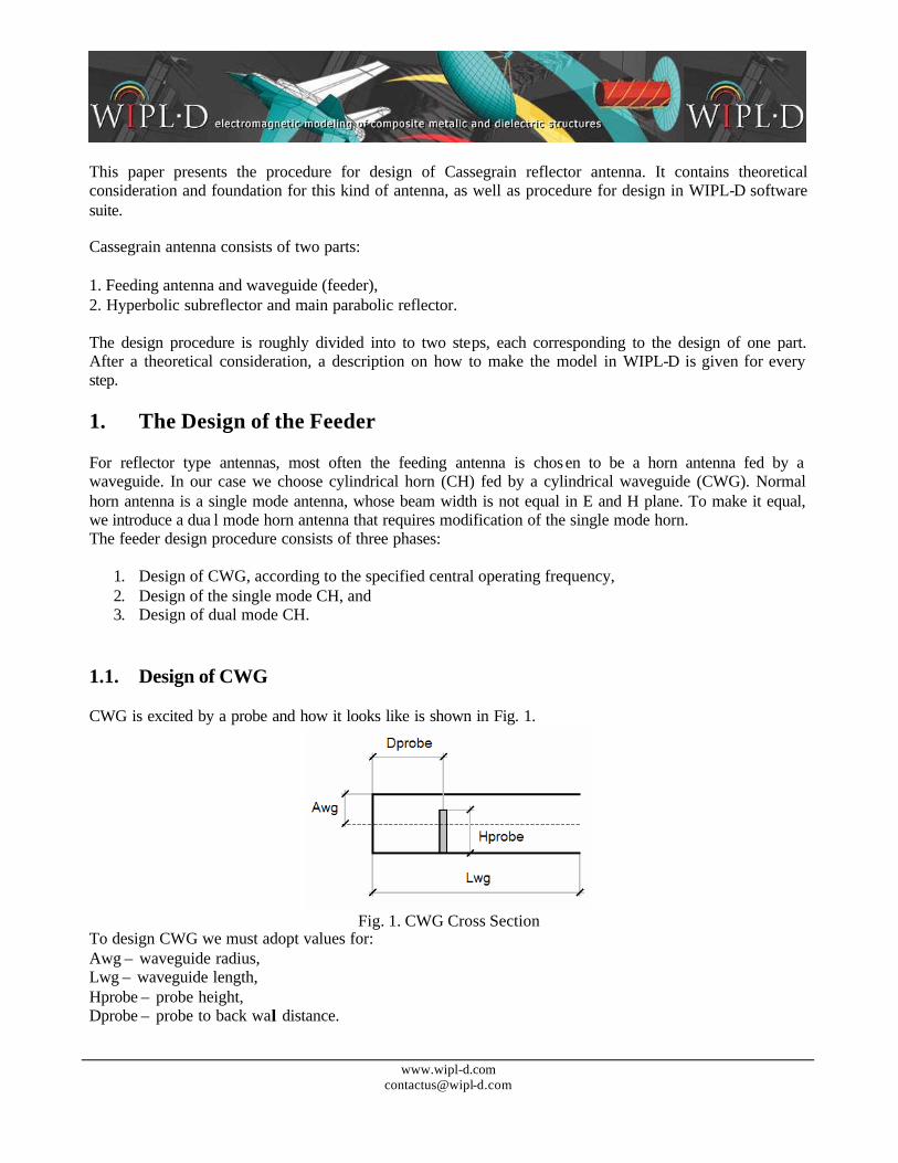
1.1. Design of CWG CWG is excited by a probe and how it looks like is shown in Fig. 1.

Fig. 1. CWG Cross Section

To design CWG we must adopt values for: Awg – waveguide radius, Lwg – waveguide length, Hprobe – probe height, Dprobe – probe to back wall distance.


The fundamental mode propagating through a cylindrical waveguide is TE11 mode. The next mode is TM10. Cut off frequencies for TE11 and TM10 modes are given with:

Awgc

TEFc 293.0)( 11 = (1)

Awgc

TMFc 383.0)( 10 = (2)

where c is the speed of light and Awg is the radius of the cylindrical waveguide. The operating frequency F0 is best chosen to be geometrical mean value of two cut off frequencie s:

Awgc

TMFcTEFcF 335.0)()(0 1011 == (3)

Taking sm

c 810= from (3) we obtain the radius of the cylindrical waveguide for given operating frequency:

][0100

][GHzF

mmAwg = (4)

At operating frequency F0 the wavelengths in free space WL0 and in the waveguide WLwg are given with:

][0300

00

0GHzF

WLFc

WL =⇒= (5)

][0619

0)(

1

02

11GHzF

WLwg

FTEFc

WLWLwg =⇒

−

= (6)

Waveguide length is chosen in such manner that higher order modes completely vanish by the open end. It is sufficient to take:

][43

][ mmWLwgmmLwg = (7)

The distance of the probe from the back waveguide wall should be:

][41

][ mmWLwgmmDprobe = (8)


The probe length should be:

][041

][ mmWLmmHprobe = (9)

The dimensioning of the waveguide is completely done. 1.2. Design of Single Mode CH CH is completely described with its length Lhorn and aperture radius Ahorn. The cross section of the cone is shown in Fig. 2. The part of this cone outlined black is a CH.

Fig. 2. Cross section of the CH

Given the 10 dB beamwidth it is possible to determine required aperture radius as:

][066][066 mmWLBW

mmAhornAhornWLBW

oo =⇒= (10)

Minimum length of the cone can be obtained from:

][07.0][][)(

22

min mmWLmmAhornmmLcone = (11)

Corresponding minimum horn length can be found from:

22

minmin )()(1)( AwgAhornLconeAhornAwgLhorn −−

−= (12)


Actual horn length is taken to be the multiple of the minimum length:

min)(LhornCLhorn= (13) where for single mode horn C should be between 1.25 and 1.5, while for dual mode it should be between 2.5 and 3. To suppress back radiation a choke is added to the horn aperture edge. A horn with a choke looks like in Fig. 3.

Fig. 3. Cross section of the CH with choke The choke length should be:

4][0

][mmWL

mmLchoke = (14)

while the choke width Dchoke is taken to be equal to metallic wall thickness T.


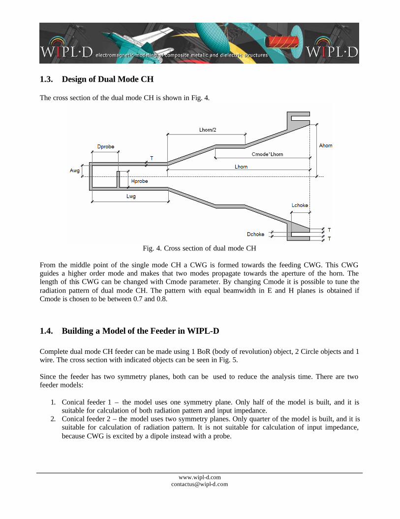
1.3. Design of Dual Mode CH The cross section of the dual mode CH is shown in Fig. 4.

Fig. 4. Cross section of dual mode CH

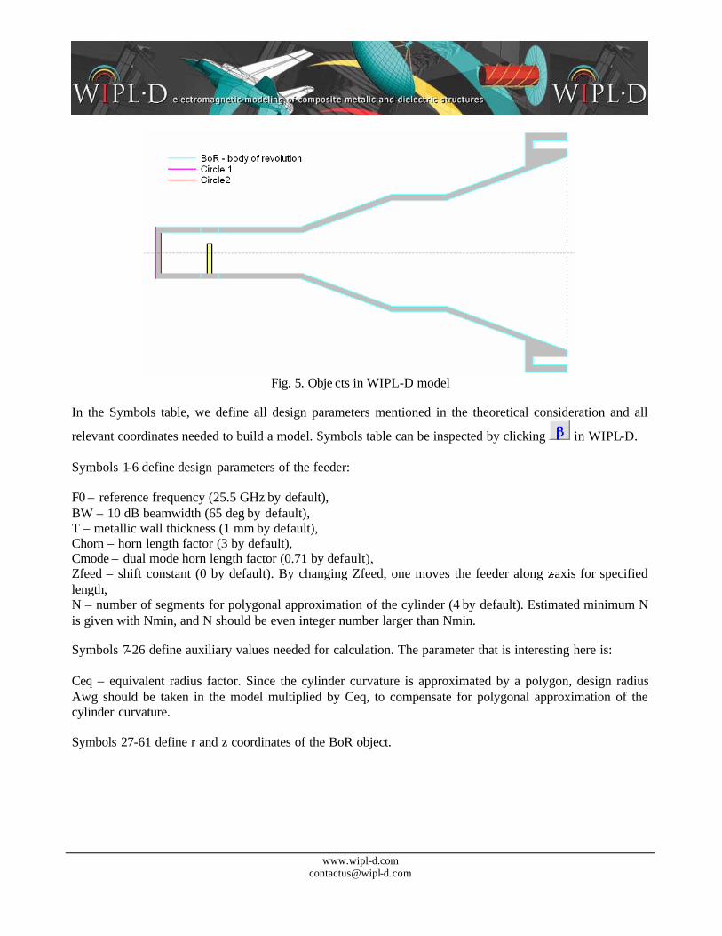
From the middle point of the single mode CH a CWG is formed towards the feeding CWG. This CWG guides a higher order mode and makes that two modes propagate towards the aperture of the horn. The length of this CWG can be changed with Cmode parameter. By changing Cmode it is possible to tune the radiation pattern of dual mode CH. The pattern with equal beamwidth in E and H planes is obtained if Cmode is chosen to be between 0.7 and 0.8. 1.4. Building a Model of the Feeder in WIPL-D Complete dual mode CH feeder can be made using 1 BoR (body of revolution) object, 2 Circle objects and 1 wire. The cross section with indicated objects can be seen in Fig. 5. Since the feeder has two symmetry planes, both can be used to reduce the analysis time. There are two feeder models:

1. Conical feeder 1 – the model uses one symmetry plane. Only half of the model is built, and it is suitable for calculation of both radiation pattern and input impedance.

2. Conical feeder 2 – the model uses two symmetry planes. Only quarter of the model is built, and it is suitable for calculation of radiation pattern. It is not suitable for calculation of input impedance, because CWG is excited by a dipole instead with a probe.


Fig. 5. Obje cts in WIPL-D model

In the Symbols table, we define all design parameters mentioned in the theoretical consideration and all

relevant coordinates needed to build a model. Symbols table can be inspected by clicking in WIPL-D. Symbols 1-6 define design parameters of the feeder: F0 – reference frequency (25.5 GHz by default), BW – 10 dB beamwidth (65 deg by default), T – metallic wall thickness (1 mm by default), Chorn – horn length factor (3 by default), Cmode – dual mode horn length factor (0.71 by default), Zfeed – shift constant (0 by default). By changing Zfeed, one moves the feeder along z-axis for specified length, N – number of segments for polygonal approximation of the cylinder (4 by default). Estimated minimum N is given with Nmin, and N should be even integer number larger than Nmin. Symbols 7-26 define auxiliary values needed for calculation. The parameter that is interesting here is: Ceq – equivalent radius factor. Since the cylinder curvature is approximated by a polygon, design radius Awg should be taken in the model multiplied by Ceq, to compensate for polygonal approximation of the cylinder curvature. Symbols 27-61 define r and z coordinates of the BoR object.


Modification of the models is easy. Starting from either from Conical feeder 1 or 2, it is possible to obtain:

1. Single mode CH - by deleting (R5,Z5), (R6,Z6), (R15,Z15) and (R16,Z16) in BoR object. 2. CH without metal thickness – by deleting from (R13,Z13) to (R18,Z18) in BoR object and by

completely deleting Circle 2 object. 3. CH without choke – by deleting from (R9,Z 9) to (R14,Z14) in BoR object

To run simulation click . After simulation is done, to inspect YZS click , and for radiation pattern

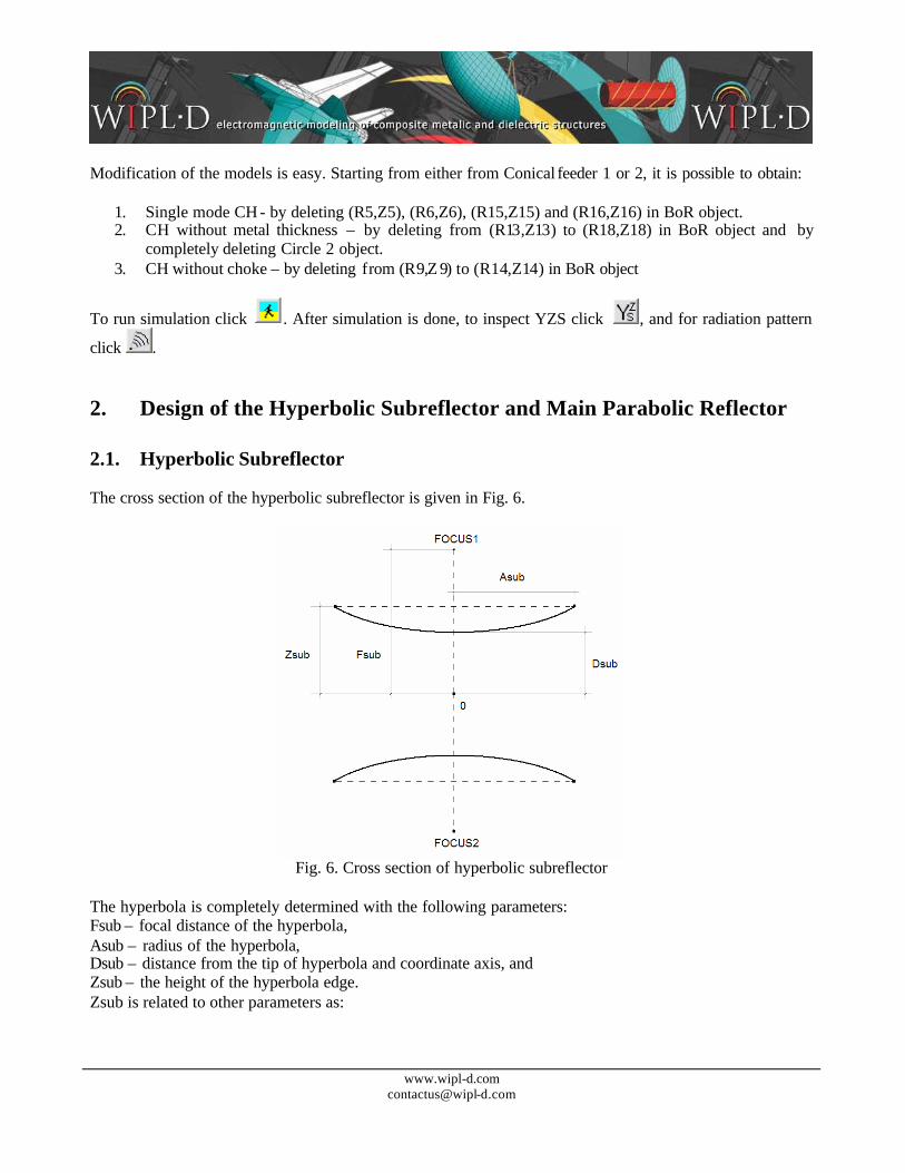
click . 2. Design of the Hyperbolic Subreflector and Main Parabolic Reflector 2.1. Hyperbolic Subreflector The cross section of the hyperbolic subreflector is given in Fig. 6.

Fig. 6. Cross section of hyperbolic subreflector

The hyperbola is completely determined with the following parameters: Fsub – focal distance of the hyperbola, Asub – radius of the hyperbola, Dsub – distance from the tip of hyperbola and coordinate axis, and Zsub – the height of the hyperbola edge. Zsub is related to other parameters as:


22

2

1DsubFsub

AsubDsubZsub

−+= (15)

Only the upper hyperbola is necessary for antenna design. The phase center of the dual mode CH should be placed in the Focus 2 of the hyperbola.

2.1. Parabolic Reflector The cross section of the parabolic reflector is given in Fig. 7.

Fig. 7. Cross section of parabolic reflector

The parabola is completely determined with the following parameters: Fref – focal distance of the parabola, Aref – radius of the parabola, Zref – the height of the parabola edge. Zref is related to other parameters as:

FrefAref

Zref4

2

= (16)

The Focus 1 of the hyperbola should be put in the focus of the parabola.


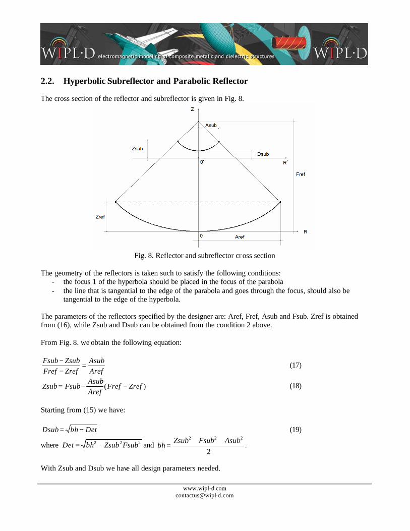
2.2. Hyperbolic Subreflector and Parabolic Reflector The cross section of the reflector and subreflector is given in Fig. 8.

Fig. 8. Reflector and subreflector cr oss section

The geometry of the reflectors is taken such to satisfy the following conditions:

- the focus 1 of the hyperbola should be placed in the focus of the parabola - the line that is tangential to the edge of the parabola and goes through the focus, should also be

tangential to the edge of the hyperbola. The parameters of the reflectors specified by the designer are: Aref, Fref, Asub and Fsub. Zref is obtained from (16), while Zsub and Dsub can be obtained from the condition 2 above. From Fig. 8. we obtain the following equation:

ArefAsub

ZrefFrefZsubFsub

=−− (17)

)( ZrefFrefArefAsub

FsubZsub −−= (18)

Starting from (15) we have:

DetbhDsub −= (19)

where 222 FsubZsubbhDet −= and 2

222 AsubFsubZsubbh

++= .

With Zsub and Dsub we have all design parameters needed.


2.3. Building the Model of the Reflectors in WIPL-D The hyperbolic subreflector and parabolic reflector are built using predefined Rflct. object in WIPL-D. The model of the reflector and sub reflector can be found in projects: - cassegrain 1 (one symmetry plane used – half model) and - cassegrain 2 (two symmetry planes – quarter model). Symbols 1-5 are defined by the user and specify referent frequency and geometry of the reflectors: F0 – reference frequency (25.5 GHz by default), Aref – radius of the parabolic reflector (150 mm by default), Fref – focal distance of the parabolic reflector (112.5 mm by default), Asub – radius of the hyperbolic subreflector (26 mm by default), Fsub – focal distance of the hyperbolic subreflector (26 mm by default). Symbols 6-8 are: Nref – number of segments per quarter of circumference for parabolic reflector. Nref should be even integer larger than NrefE estimated in symbol 9. The estimation of NrefE is made using the criterion that maximum size of the plate in the model is no larger than 1.5 wavelength at reference frequency F0. Nsub – number of segments per quarter of circumference for hyperbolic reflector. Nsub should be even integer larger than NsubE estimated in symbol 10. The estimation of NsubE is made using the criterion that maximum size of the plate in the model is no larger than 1 wavelength at reference frequency F0. BWE – estimation of the beamwidth of the feeder radiation pattern in order to have 10 dB space taper at the edge of the subreflector. BW from the model of CH should be equal to BWE. Symbols 11-19 are additional symbols for geometry definition and positioning, as well as auxiliary symbols. What is left to do is to import the feeder to the reflector. There are two projects of the complete antenna: - Cassegrain with conical horn 1 (one symmetry plane - half model) – suitable for calculation of both

radiation pattern and input impedance. - Cassegrain with conical horn 2 (two symmetry planes – quarter model) – suitable for calculation of

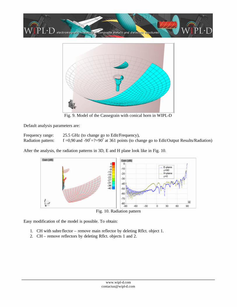
radiation pattern only. To import use option Edit/Structure/Import. After, move the feeder phase center to hyperbola focus by specifying Zfeed=Fref-2*Fsub in the Symbols table. The final model with one symmetry plane (Cassegrain with conical horn 1) looks like in Fig. 9.


Fig. 9. Model of the Cassegrain with conical horn in WIPL-D

Default analysis parameters are: Frequency range: 25.5 GHz (to change go to Edit/Frequency), Radiation pattern: f =0,90 and -90?=?=90? at 361 points (to change go to Edit/Output Results/Radiation) After the analysis, the radiation patterns in 3D, E and H plane look like in Fig. 10.

Fig. 10. Radiation pattern

Easy modification of the model is possible. To obtain:

1. CH with subre flector – remove main reflector by deleting Rflct. object 1. 2. CH – remove reflectors by deleting Rflct. objects 1 and 2.

cassegrain reflector antenna with dual mode … reflector antenna with...cassegrain reflector...

Documents