cash flows and market risk - illinois: ideals home

UNIVERSITY Of-

ILLINOIS LIBRARYAT URBANA-CHAMPAIGN

BOOKSTACKS

H

& /--3

m H

H

nfi

(t-i

CD00

O

Digitized by the Internet Archive

in 2011 with funding from

University of Illinois Urbana-Champaign

http://www.archive.org/details/cashflowsmarketr855gent

/•' -^^

FACULTY WORKINGPAPER NO. 855

Cash Flows and Market Risk

James A. Gentry, Paul Newbold,and David T. Whitford

College of Commerce and Business Administration

Bureau of Economic and Business ResearchUniversity o' ilii'icis, Urbana-Champaigr

BEBRFACULTY WORKING PAPER NO. 855

College of Commerce and Business Administration

University of Illinois at Urbana-Champaign

March 1982

Cash Flows and Market Risk

James A. Gentry, ProfessorDepartment of Finance

Paul Newbold, ProfessorDepartment of Economics

David T. Whitford, Assistant ProfessorDepartment of Finance

Abstract

The theory of finance recognizes that the value of any asset is

based upon the risk-adjusted present value of its expected future net

cash flows. Recently Fama has modeled a multiperiod pricing process

based upon the capital asset pricing model (CAPM) . Based upon Fama's

model, this research develops the rationale for using cash flows to

explain the value and systematic risk of a firm. It presents a model of

eight components underlying a firm's funds flows and hypothesizes how

these affect systematic risk. Finally, this research measures and

empirically analyzes the relationship between a firm's beta and levels,

trends, and variability of these eight funds flow components.

CASH FLOWS AND MARKET RISK

The theory of finance recognizes that the value of any asset is

based upon the risk-adjusted present value of its expected future net

cash flows [5, 7, 14, 22, 23]. Financial theory also presumes that the

goal of the firm is maximization of shareholder wealth. Therefore, the

management of real assets is assumed to reflect the perspective of in-

vestors, who collectively determine the value of the firm.

The capital asset pricing model (CAPM) , developed by Sharpe [20],

Lintner [15] and Black [4] (SLB) , currently lies in the main stream of

financial management thought. Initially, the market equilibrium models

of SLB and others were primarily concerned with one-period rates of re-

turn on a firm's common stock, where the length of the period was unde-

fined. During its formative years the CAPM did not focus on a multi-

period stream of cash flows generated by a firm's investments nor the

effect that an uncertain stream of cash flows would have on the price

of a firm's securities. However, in 1977 Fama [10] modeled a multi-

period pricing process that utilized the SLB framework. The key contri-

bution of Fama's article was that a firm's beta coefficient was related

to the risks inherent in its cash flows. Fama showed that cash flows

can vary in a multiperiod SLB model and that a single risk-adjusted

discount rate can be applied to all flows [10, p. 4].

The Fama study provides the theoretical framework for further re-

search on the relationship between the firm's beta coefficient and the

risks of the cash flows generated by the firm's real assets. Several

authors [1, 2, 3, 6, 9, 16, 17, 18, 19, 21] have attempted to identify

-2-

and measure the relationship between an ad_ hoc set of financial variables

and beta. In general the findings have been mixed and inconclusive.

The lack of explanatory power of the previous models occurs in part be-

cause a theoretical valuation framework was not properly specified and

an ad^ hoc set of variables was used to test the model.

This study is based on the widely accepted theory that relates the

value of the firm to its long run stream of net cash flows from real

assets. The objectives of this paper are to develop the rationale for

using cash flow information for explaining the value and market (syste-

matic) risk of a firm; to present a model of eight components underlying

a firm's funds flows; to present a set of scenarios that highlight

classic funds flow patterns and hypothesize their effect on a firm's

systematic risk; to measure empirically and analyze the relationship

between a firm's beta coefficient and the eight funds flow components;

and finally to summarize the implications of the empirical findings for

financial management and planning.

WHY CASH FLOWS?

In 1937 John Burr Williams created the theory for valuing common

stock [25]. Williams constructed the theory on the concept that the

payment of cash dividends to investors for an endless time period was

the basis of a common stock's value. Discounting the stream of cash pay-

ments to investors at the appropriate rate provided a solid theoretical

base for determining the value of a firm's common stock.

In a related context, the present value of net cash flows from a

capital investment is used to establish the acceptability of an invest-

ment project [5, 7, 14, 22, 23]. Although there are many simplifying

-3-

assumptions involved in estimating future cash inflows and outflows,

financial economists recognize net cash flows are a basic component in

determining the value of a capital investment and a common stock. The

actual measurement of the cash flows rely on accrual accounting infor-

mation.

As noted earlier, many empirical studies have attempted to discover

the components underlying a firm's systematic risk or beta. The find-

ings of the various studies ranged from mixed to inconclusive. One ex-

planation for the mixed results is that the previous studies have not

provided a theoretical framework that links market risk with a particu-

lar set of financial ratios. This study focuses on the relationship

between the level of a firm's systematic risk and the relative size and

variability of eight corporate funds flow components. Use of funds flows

provides two distinct advantages. First, they are unambiguous com-

ponents of a firm's market value. Second, they reflect the success

management has experienced in controlling and directing the real assets

of the firm.

In theory actual cash flow data would provide the best information

to use in an empirical analysis of the determinates of a firm's market

9risk. Unfortunately actual cash flow data are not publicly available.

The next best source of data are funds flows generated from balance sheet

and income statement information. The model we have used to identify

funds flow measures was developed in 1972 by Erich Helfert [12].

Helfert's model integrates balance sheet and income statement informa-

tion and subdivides the funds flow variables into the three natural

decision areas: investment, financing and operations.

-4-

The concept of funds flow analysis is designed to display movement

of resources in financial terms. The funds flow statement measures the

inflow of funds and tracks their outflows much like the traditional

sources and uses of funds statements. By analyzing a company's chrono-

logical trends and patterns of funds flow, one can detect the various

ways that management policies and decisions affect a company's finan-

cial performance. The funds statement can be used to compare the in-

ternal flow of resources among divisions or to compare differences and

similarities of competitors. It can also be used to measure historical

performance or alternatively, to evaluate the performance of alternative

planning strategies from pro forma financial statements. In summary,

a primary objective of funds flow analysis is to provide chronological

benchmarks for measuring and judging management effectiveness [12, p. 4].

Helfert's funds flow statement integrates the sources and uses of

funds from the balance sheet together with the inflow and outflow of

funds from the income statement. Because the balance sheet reflects

the measurement of assets and liabilities at a single point in time, to

calculate the change in the movement of funds it is necessary to measure

the change between time periods

.

Although the changes in the balance sheet reflect major movements

in the stock of assets and liabilities, there are also flow items that

are required to have a complete picture of total sources and uses of

funds within the firm. The major source of funds is net sales. Also

interest and other income items received are sources of funds. The ma-

jor outflow items are operating costs such as materials, supplies, labor,

power and other cost items. Also variable and fixed overhead costs

.-5-

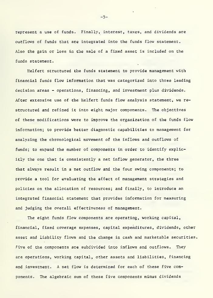
represent a use of funds. Finally, interest, taxes, and dividends are

outflows of funds that are integrated into the funds flow statement.

Also the gain or loss in the sale of a fixed asset is included on the

funds statement.

Helfert structured the funds statement to provide management with

financial funds flow information that was categorized into three leading

decision areas - operations, financing, and investment plus dividends.

After extensive use of the Helfert funds flow analysis statement, we re-

structured and refined it into eight major components. The objectives

of these modifications were to improve the organization of the funds flow

information; to provide better diagnostic capabilities to management for

analyzing the chronological movement of the inflows and outflows of

funds; to expand the number of components in order to identify explic-

itly the one that is consistently a net inflow generator, the three

that always result in a net outflow and the four swing components; to

provide a tool for evaluating the affect of management strategies and

policies on the allocation of resources; and finally, to introduce an

integrated financial statement that provides information for measuring

and judging the overall effectiveness of management.

The eight funds flow components are operating, working capital,

financial, fixed coverage expenses, capital expenditures, dividends, other

asset and liability flows and the change in cash and marketable securities,

Five of the components are subdivided into inflows and outflows. They

are operations, working capital, other assets and liabilities, financing

and investment. A net flow is determined for each of these five com-

ponents. The algebraic sum of these five components minus dividends

-6-

and net fixed coverage expenses will equal the change in cash and market-

able securities. The revised format for the funds flow analysis and the

acronyms for each variable are presented below.

Operating FlowsInflows (01)

minus : Outflows (00)equals: Net Operating Funds Flow (NOFF)

Working Capital FlowsInflows (WCI)

minus: Outflows (WCO)

equals: Net Working Capital Funds Flows (NWCFF)

Other A&L FlowsInflows (OA&LI)

minus: Outflows (OA&LO)equals: Net Other A&L Funds Flow (NOA&LF)

Financial FlowsInflows (FI)

minus : Outflows (FO)

equals: Net Financial Funds Flow (NFFF)

Investment FlowsInflows (II)

minus: Outflows (10)

equals: Net Investment Funds Flow (NIFF)

Dividend Outflows (DIV)

Fixed Coverage Expenditure Outflows (FCEF)

Change in Cash (CC) [Below: equals the sum of preceding sevencomponents]

Beginning Cash and S.T. Investments

Ending Cash and S.T. Investments

REVISED MODEL

The funds flow components contained in the revised Helfert model

are presented in equation 1. Because the interrelationship among the

components is complex, equation (1) is presented in a format of a most

likely case.

-7-

NOFF - NWCFF + NFFF - FCEF - NIFF - DIV ± MOA&LE ± CC = . (1)

Net operating funds flows (NOFF) are composed of all operating in-

flows (01) , of which sales is the primary source, minus all operating

outflows (00) . The primary operating outflows are expenditures related

to the cost of goods sold, selling and advertising taxes, research and

development, rental, extraordinary, minority interest, deferred taxes,

investment credit and tax loss carry forward. In summary,

NOFF =01 - 00 , -J I .t-'m'.'! >.ft . (2)

where 01 > 00 .

Normally, NOFFs are the primary source of funds inflow. However, sea-

sonal and/or random events may cause NOFFs to be negative, which repre-

sents an outflow or a use of funds. Also declining market share or size

of market, or internal operating inefficiencies may cause NOFFs to be

negative. Equation (2a) illustrates a negative NOFF.

-NOFF =01 - 00 , (2a)

where 01 < 00

Net working capital funds flow (NWCFF) can be either a use or a source

of funds. A net outflow of funds for working capital occurs when ac-

counts receivable (AR) or inventories (INV) are increasing or when ac-

counts payable (AP) are decreasing, or a combination of both. Under

these conditions, NWCFFs are negative because they reflect an outflow

of funds. Equation (3) presents the case of NWCFFs as an outflow in equa-

tion form:

-8-

-NWCFF = AAP - AAR - AINV , (3)

where

-AAP = AP - AP , where AP < AP _ ;

AAR = AR - AR , where AR > AR ;

AINV = INV - INV , , where INV > INV ,

.

t t t-1' t t-1

Alternatively, when the level AR or INV are reduced or when AP are

increased, or both, they represent an inflow of funds and the NWCFFs are

positive, as shown in equation (4).

NWCFF = AAP - AAR - AINV , , (4)

AAP = AP - AP , where AP > AP _ ;

-AAR = AR - AR , where AR < AR ;

-AINV = INV - INV , where INV < INV _ .

During a transition in current operations, management may change the

level of AR, INV, and AP. Thus working capital funds provide management

a buffer to adjust the funds flow in order to maintain an equilibrium

condition between sources and uses.

If net investment flows (NIFF) are financed totally by operating

funds, the firm does not need to utilize financial leverage. Equation

(5) represents this condition, where NOFFs are the source of funds and

NIFFs the uses.

NOFF = NIFF . (5)

This condition reflects a firm in a strong competitive position, for

example a firm that has a dominant share of a growing market. As an aid

-9-

in understanding equation (5) , a graphic presentation is shown in

Exhibit 1 as scenario 1. The NOFFs and NIFFs in scenario 1 are in-

Insert Exhibits 1 and 2 here

creasing over a five year period. The data in Exhibit 1, for scenario

1, are presented in Exhibit 2 as proportions of the total, e.g.,

NOFFs = 100% and NIFFs = 100%. Under these conditions it is hypo-

thesized that a firm's market risk measure, beta, would be rela-

tively low.

\n\en a firm's internal operating funds are insufficient to meet

the investment outflows, external debt, or equity, the major components

of net financial funds flow (NFFF) may be sold to finance the shortfall

in funds. When debt is utilized, interest is paid and defined as a

fixed coverage expenditure flow (FCEF) . Interest will always be an out-

flow (use) of funds, and usually NIFFs will be an outflow. Thus each

has a negative sign in equation 1. When debt or equity are being in-

creased, NFFFs are an inflow of funds (a source) which is reflected as

a positive value in equation 1. This scenario is presented in equation

(6) where the components on the left hand side (LHS) of the equation are

sources of funds and the right hand side (RHS) are uses:'

NOFF + NFFF = NIFF + FCEF . " (6)

Scenario 2 in Exhibits 1 and 2 portrays a graphic description of the

mixed debt/equity strategy. Exhibit 2 clearly shows the presence of

a 50/50 debt/equity strategy for scenario 2. We hypothesize a firm's

-10-

beta for strategy 2 will be greater than scenario 1 because financial

risk was introduced through the sale of debt.

In Exhibits 1 and 2, scenario 3 depicts a firm that uses internal

NOFFs to finance its investment in plant and equipment and working

capital. Also NOFFs are used to pay dividends. In this example, NIFFs,

NWCFFs, and DIVs reflect an outflow of funds (a use). Scenario 3 de-

scribes a firm with a strong debt/equity position. It is presented in

equation (7) where the LHS represents the source of funds and the RHS

contains the uses of funds,

NOFF = NIFF + NWCFF + DIV . (7)

If dividend or working capital decisions create investor uncertainty

in the stock market, the beta for scenario 3 will be higher than in

scenario 1. Additionally, if the risk caused by dividend or working •

capital expenditures in scenario 3 is less than the financial risk

created in scenario 2, the market beta will be lower in scenario 3,

and, of course, vice versa.

When operating funds flow are relatively unstable, there can emerge

investment and financing policies analogous to the scenario presented in

scenario 4 in Exhibits 1 and 2. Equations (8a) and (8b) reflect a com-

plex, mixed strategy illustrated, for example, in time periods 2 and 4,

where the LHS is sources and the RHS is uses of funds:

and

NOFF + NFFF + CC„ = NIFF + NWCFF + FCEF^ + DIV^ (8a)

NOFF, + NWCFF, = DIV, + CC, + FCEF, + NFFF.

,

(8b)4 4 4 4 4 4

-11-

Equation (8a) shows how management utilizes three major buffer ac-

counts to adjust the flow of funds and maintain an equilibrium between

sources and uses of funds. The three primary buffer accounts are NWCFFs,

NFFFs, and change in cash and marketable securities (CC) . Net other

assets and liabilities (NOA&LF) is also a buffer component, but for

simplicity it is not presented in Exhibits 1 and 2. In (8a) the CC is

a source of funds and thus would have a positive sign in equation (1)

.

However, in equation (8b), CC is a use of funds or an outflow, and would

have a negative sign in equation (1) . Also in equation (8a) NWCFFs are in-

creasing and thereby using funds. However, in (8b), working capital pro-

vides funds along with NOFFs, which allows management to retire debt

(NFFF) . Exhibit 2 captures the subtle changes developed in scenario 4.

Equation (9a) illustrates how NFFF can be a source of funds and (9b)

depicts NFFFs as a use of funds for retirement.

NFFF = STBF + LTBF + CSF , (9a)

where

STBF = an increase in short-term borrowing in period t;

LTBF = an increase in long-term borrowing;

CSF = an increase in common stock outstanding.

Any two of the above units could be zero and NFFFs would be positive if

the third unit increased. However if any one of the units of NFFFs was

negative and the others were zero, or if the algebraic sum of the three

were negative, e.g., when debt or equity is retired, NFFF is negative

as illustrated in equation (9b)

.

-12-

, -NFFF = -STBF - LTBF + CS, (9b)

where

-STBF = a decrease in short-term borrowing;

-LTBF = a decrease in long-term borrowing;

CS = an increase in common stock that is less than the sum ofSTBF and LTBF.

In scenario 5, found in Exhibits 1 and 2, we find a firm that has

rapidly declining net operating flows over the five year period. In

fact, NOFFs are negative in year 5. This rapid decline is primarily

offset by financing flows, but also there is a reduction in cash and

in net working capital to make up the remaining shortfall.

The outflow side of the scenario reflects a firm with declining in-

vestment, except in year 4, and rising fixed charges that are directly

related to the increase in debt financing. The firm continues to pay

dividends through year 3 even though net operating flows are declining.

Scenario 5 reflects a firm in a declining financial condition.

Year 5 captures the worst case where NFFFs are the total source of funds

and NOFFs are outflows. Equation (10) depicts year 5 in strategy 5.

NFFF = NIFF + NOFF + FCEF + NWCFF (10)

The fund scenario presents a firm that is experiencing a different

form of financial decline. In scenario 6, the firm has a rapid deterio-

ration of NOFFs and increasing reliance of NFFFs in year 2 and 3. In

year 4 and 5 the sale of fixed assets is necessary to offset the outflow

for operations and financing. This is a severe strategy because the firm

-13-

is forced to sell plant and equipment which is the economic base upon

which operating flov7S are generated.

EMPIRICAL ANALYSIS

The objective of the empirical analysis is to test the relation-

ship between a company's market risk, (beta) and relative measures of

each funds flow component. Before this is accomplished, there is a

need to measure the level and trend of each funds flow series, because

both measures contribute to the explanation of the behavior of the series

[8] . Additionally there is substantial evidence that time series ac-

counting data are either a random walk series or a random walk with a

drift [13].

Data Sample

The 1980 Fortune 1000 manufacturing companies are the company pop-

ulation for the empirical analysis. These 1000 corporations were grouped

into four quartiles of 250 companies, based upon the level of 1979 sales,

e.g., the first group contained companies ranked 1-250 according to

sales; the second group contained companies 251-500, the third and

fourth groups were ranked 501-750 and 751-1000, respectively. From the

first three sets of companies— (1-250) , (251-500), and (501-750)~a

sample of 30 companies per group were randomly selected for a total of

90 companies. From companies numbered 751-1000, only 24 companies met

the designated sample criteria. There were 114 companies in the total

sample.

The following criteria were used in selecting these 114 companies.

Each company had to be on the COMPUSTAT Annual Industrial file and

-14-

contain complete annual financial statement data for the period 1969-1979.

The monthly data for the period 1970-1979 had to be available on the

monthly return tapes compiled by the Center for Research on Security

Prices at the University of Chicago (CRSP) . Finally, each company's

fiscal year had to end on December 31. This last criterion allowed

all betas and funds flow variables to be measured over the same period.

To provide an overview of the statistical results. Exhibit 3 pre-

sents a summary of the means and standard deviations for each of the

Insert Exhibit 3 here

eight funds flow components for the sample companies. Also the mean of

the total flow, i.e., all sources and/or uses, divided by total asset

ratio and the mean beta of the 114 companies are found in Exhibit 3.

The data in Exhibit 3 show that net operating funds flow (NOFF) are the

primary source of inflow. On average, NOFF contributes 67 percent of

the total inflows, ±11.3 percent. On the outflow side, net invest-

ment funds flow (NIFF) was the largest component with 34 percent of the

total, ±14 percent. Additionally, interest represents approximately

13 percent of the total outflow, ±7 percent, and dividends compose

12 percent, ±8 percent, of total outflows. The mean beta of the 114

companies was 1.27, ±.32.

There is a marked difference in the percentage contribution of

each funds flow component when comparing the ten highest risk companies

to the ten lowest risk companies from the sample of 114. The data for

this comparison are presented in Exhibits 4 and 5. The companies are

Insert Exhibits 4 and 5 here

-15-

ranked in descending order of their respective beta coefficients. The

mean beta for the ten companies with the highest risk was 1.87 compared,

to a beta of .75 for the ten lowest risk companies. The mean size of

the ranking in the Fortune 1000 was 678 for the highest risk set and

348 for the lowest risk companies. The high risk companies contribute

only 57 percent of total inflows from operations vis-a-vis 76 percent

for the low risk companies. Net investment funds flow represented

32 percent of total outflows of the riskier companies, and 38 percent

for the lower risk firms. The lower risk companies pay out 8 percent

of total flows in interest compared to the 16 percent for the riskier

companies. The opposite occurs with dividends. The ten highest risk

companies pay out only 5 percent of total flows in dividends while the

ten lowest risk companies distribute 21.7 percent of the total outflows

in dividends. For both risk groups working capital was a user of funds,

8.7 percent of total outflow of highest risk set and 0.9 percent for

lowest risk group. Finally, financing composed 1 percent of the total

inflow for the lowest risk group and 3.7 percent for the highest cell.

Given the trends revealed in Exhibits 4 and 5, further investiga-

tion of the relationships between fund flow components and the level of

systematic risk is warranted. Multiple regression is utilized to ex-

amine specific relationships. First, the relationship between the

relative levels of the eight flow components given in equation (1)

and market risk are tested. Next time series trends in the relative

levels of the components are analyzed. Finally, variability measures

of these flows are investigated.

-16-

The first phase of the study is given in equation (11).

Beta. = bg + b^TA. + b^TF/TA. + b3X.^^ + b^X.^2 ^ ^^5^.3 ^^6î,4

^ ^î,5 -^ ^8^.6 -^ Vi,7 ^ ^0î,8 ^ \ (11)

In (11), the following definitions are appropriate:

Beta. = the ith company's market risk measure derived fromthe capital asset pricing model (CAPM) . Beta.

2"

equals cov(i,m)/a or the covariance between rate

of return of the ith company's common stock andthe return on the market, divided by the variance of

market's return.

TA. = the mean level of ending total assets for firm i

during the 10 year study period;

TF./TA. = the mean level of total flows (total sources or uses)relative to ending total assets for firm i, i.e.,

TF /TA = {(TF /TA ) + (TF /TA ) + ... +

X. - = NOFF./TF. = Z (NOFF. /TF. )/N mean level of net1,1 1 1

^.^ji^

' i,t i,t'

operating funds flow for the ith company divided bytotal flow for the (N=10) period 1970-1979. Notethat TF. equals the total flow (i.e., funds sources)

for firm i in period t; NOFF. is net operating

funds flow for firm i during period t;

X. „ = NWCFF./TF., the ith firm's mean level of net working1,2 11

capital funds flows relative to total flows, i.e.,

NWCFF./TF. = {(NWCFF. ,/TF. ,) + (NWCFF. „/TF. „)1 1 1,1 1,1 1,2 1,2

+ ... + (N^^^CFF.^^q/TF.^^q} . 10;

X. _ = NOA&LE./TF., the ith firm's mean level of other asset and1,3 11

liabilities funds flow relative to total flows, i.e..

NOA&LF./TF. = {(NOA&LF. /TF. ) + (NOA&LF. „/TF. „)

+ ... + (NOA&LF. ^^q/TF.^^q)} . 10;

-17-

X = NFFF./TF., the ith firm's mean level of net financial

funds flow relative to total flows, i.e..

NFFF./TF. = {(NFFF. /TF. ) + (NFFF. /TF. ) + ... +

(NFFF.^^q/TF.^^q)} .10;

X. c = -NFEF./TF., the ith firm's mean level of fixed coverage

expenses relative to total flows, i.e..

NFEF./TF. = {(NFEF. /TF. ) + (NFEF. /TF. )+..„+

(NFEF.^^q/TF.^^q)} .10;

X. ^ = -NIFF,/TF., the ith firm's mean level of net investment1,6 1 1

funds flow expenditures relative to total flows, i.e.,

NIFF./TF. = {(NIFF. /TF. ) + (NIFF. /TF. ) + ... +X X XyX XyX A. y ^ A. y Z.

(NIFF.^^q/TF.^^q)} . 10; ,

X. _ = -DIV./TF., the ith firm's mean level of dividend outflows1,7 1 1

relative to total flows, i.e..

DIV /TF = {(DIV. /TF. ) + (DIV. /TF. )+...+X X XyX X*X Xa^ Xk^

(°^^.io/î,io>> ' ^0'

X. „ = CC./TF., the ith firm's mean level of change in cash and1,8 11 ^

marketable securities relative to total flows, i.e..

CC./TF. = {(CC. /TF. ) + (CC. /TF. ) + ... +X X XjX XbX X«^ Xk^

(^î.io/Tî,io)> ^1°' ^^^

T\- - the OLS error term for the ith company.

As seen in equation (11) two scale variables, average total assets

and average total flow relative to ending total assets, were included.

These two variables are included to capture the importance of asset size

the productivity of those assets through the ratio of total flows/to

total assets.

-18-

In testing equation (11) certain a_ priori relationships seem reason-

able. For example, larger firms should have, other things equal, lower

betas. Also firms with large operating funds flows and a major cushion

of liquid assets should be less risky. In contrast, growth firm with low

dividends and high capital expenditures would have higher betas. The

same would be true of firms with large fixed coverage expenses and large

levels of positive financial flows generated primarily through issuing

debt. Unfortunately the relationships between other variables are some-

what ambiguous. Large working capital and other assets and liability

flows might indicate strong growth potential and higher levels of

systematic risk. However, if these buildups are indicative of inventory

accumulation due to lack of consumer acceptance of a firm's products, a

slowdown in growth might be indicated.

In performing the regression analysis outlined in (11) , there arose

a problem of statistical overidentification. In turn this problem

raised questions regarding the a_ priori relationships between beta and

various flow categories. The overidentification problem occurred because

the sum of the relative flow components in any given year equal zero.

Although the 10 year average flow proportions do not necessarily sum to

zero, in the regression average source proportions are balanced against

average use proportions. To prevent overidentification, one of the funds

flow components is omitted from the regression. The excluded variable

serves as an offsetting source or use against each of the remaining flow

variables.'

The results of the relative flow regressions are presented in

Exhibit 6. The coefficients measure the effect each flow component has

-19-

on beta. That is an increase in a flow component is used to fund the


balancing use component in each row, or vice versa. Because fixed cov-

erage expenses, capital expenditures, and dividends are outflows, the

sign of these coefficients are reversed.

Only the upper diagonal parameters are presented in Exhibit 6.

Lower diagonal parameters would of course have the same value (with

opposite sign) of their counterparts in the upper diagonals. As an

example the coefficient (t-value) in the -DIVIDENDS row and the CC

column would be -2.090 (-3.16). Also the coefficient (t-value) in the

-CAPITAL EXPENDITURE row and CC column would be -.276 (.47). Following

this procedure the coefficient rows (with opposite signs) can be rotated

down to fill the appropriate columns.

For each regression in Exhibit 6 the intercept term, the coefficients

of TA and TF/TA, the adjusted R , and F-value are identical. The rela-

tive flow measures explain approximately one-third of the variation in

the level of systematic risk. Both average total assets and the average

ratio of total flows to total assets have negative coefficients. However

neither is significant at the 5 percent level. As hypothesized, the NOFF

column coefficients are negative, but only the trade-off between NOFF

and DIV is statistically significant. The coefficients of the swing

components, NWCFF and NOA&LF, coefficients vary in sign. As in the NOFF

trade-off, only the DIV balancing flow is statistically significant.

An analysis of the dividend row indicates that all coefficients except

the fixed coverage outflow are significant at the 1 percent level. Most

-20-

of the signs of the coefficients in the dividend row are intuitively

appealing. Whenever dividends are funded by operations or by reductions

in working capital, other assets and liabilities or liquid assets, sys-

tematic risk falls. On the other hand when fixed coverage expenses or

capital expenditures increase necessitating a reduction in dividends,

systematic risk rises.

There are two unique trade-offs present in Exhibit 6. The param-

eters indicate when net financial inflows are used to finance dividends,

systematic risk drops. In addition, when net financial funds flows are

used to finance fixed coverage expenses, systematic risk also falls.

Although these findings suggest financial irresponsibility, an alterna-

tive explanation seems plausible. Firms that use prudent amounts of

financial leverage to increase the return on equity can also generate

increased dividends. Although financial leverage should increase sys-

tematic risk, sustainable increase in dividends should reduce a firm's

beta. The evidence in Exhibit 6 indicates that the trade-off between

higher debt and larger dividend growth results in lower systematic risk.

The NFFF-FCEF trade-off is interesting, and at least two possible

explanations exist. If a corporate borrower were to encounter a serious

cash flow crisis its lenders might willingly restructure debt agreement.

Exhibit 6 indicates that if^ lenders are willing to finance fixed coverage

expenses, the level of systematic risk borne by shareholders will de-

cline. An alternative explanation for the NFFF-FCEF effects on market

risk might be attributed to the fact that the firms that use fixed-coupon

long-term debt in an inflationary environment benefit when actual infla-

tion exceeds expectations.

-21-

The second phase of the investigates the relationship between sys-

tematic risk and trends in the relative funds flow components over time.

Trends in the X. (i=l,...8) ratios, given in equation (11), were calcu-

lated using OLS regression techniques for the period 1970-1979. In these

regressions the dependent variable was the relative flow component; time

was the independent variable.

The structure of the trend model is given in equation (12)

.

Beta. = b„ + b^TA. + b-T„„,„. . + b»T^ ^ + b, T^ . + b^T^ _ + b,T^,1 1 1 2 TF/TA,i 3 X.,1 4 X.,2 5 X. ,3 6 X. ,4

1 i' i' i'

+ ^'^X..5 + Vx.,6 + Vx.,7 + ^OTX.,8 + ^ (^2)1 1 1 i'

In (12) the T variables are trends of the appropriate flow compon-

ents. The results of this phase of the analysis are given in Exhibit 7=


The interpretation of the coefficients in Exhibit 7 is similar to those

in Exhibit 6. However, instead of a pure sources/uses trade-off, the

coefficients measure the impact upon systematic risk of downward or up-

ward trends in sources and usages of funds flow proportions.

In Exhibit 7 the intercept as well as T_^,„. . and TA. coeffi-TF/TA,i 1

cients were the same in each regression. However, unlike the levels

analysis, average total asset size is negatively and significantly re-

2lated to levels of systematic risk. The adjusted R for the trend

regressions is slightly below 20 percent, and the overall set of inde-

pendent variables in these regressions is significant at the 5 percent

level.

-22-

The majority of the coefficients in Exhibit 7 are positive. This

implies the matching of an increasing trend in fund sources against an

increase in funds usage trends to increase systematic risk. However,

relatively few of these parameters are statistically different from

zero. Trends in dividend policy have a high statistical association

with levels of systematic risk. Based upon the signs of the coeffi-

cients in the dividend row, increasing trends in net operating flows

that increase dividends will increase levels of systematic risk. The

same would be true of all other funds flow category trends excepting

cash and marketable securities.

The final phase of the empirical analysis investigates the role that

variability in funds flow components play in determining levels of sys-

tematic risk. Two variability measures were used: the standard devia-

tions of each flow category and the sum of the squared residuals obtained

from the OLS trend regressions. The results of these regressions are

reported in Exhibit 8. The standard deviation analysis indicates that


only variability in net financing flows and dividends are statistically

significant. In the OLS residual analysis average total assets and

dividends are statistically significant at the 5 percent level. Net

financing flows are significant at the 10 percent level. The adjusted

2R values for the standard deviation and residual regressions are .271

and .226, respectively. The F-values for both regressions are signifi-

cant at the 5 percent level. The negative relationship between dividend

variability and systematic risk appears to be counterintuitive. However,

-23-

if firms attempt to follow a stable dividend policy, deviations from

stable dividend growth trends should be relatively uncommon. Radical

departures from an announced dividend policy could easily be caused by

nonsystematic factors. A decline in the correlation between returns of

the market and a firm's dividend policy might very well cause a firm's

beta to drop. '^'- ' '-

The preceding analysis confirms the role that levels, trends,

and variability in funds flows components separately play in affecting "^

levels of systematic risk. However, a major question remains unanswered.

Specifically, do various combinations of levels, trends, and variability

add explanatory power when considered jointly. To answer this question,

additional regressions utilizing the dividend balancing regression var-

iables in Exhibits 6 and 7 in conjunction with residual variables in

Exhibit 8 were undertaken. Based upon a F-test, it is possible to de-

termine if the addition of a variable set adds statistically significant

explanatory power to a regression model. Using the percent flow, divi-

dend model from Exhibit 6 as a base for comparison, addition of neither

the trend nor availability sets offers a statistically significant im-

provement in explanatory power. In addition, the inclusion of both

trend and variability independent variables does not statistically im-

prove the model's explanatory power. On this basis it appears that

average levels of corporate cash and funds flows are more closely linked

levels of systematic risk.

CONCLUSIONS

A model based on valuation theory was developed to explain the

relationship between the level of a corporation's systematic risk and a

-24-

set of eight funds flow components. A set of statistical models measured

the level, trend and variability of funds flow components as explanators

of market risk. Several important observations emerged from the study.

First, cash flow to shareholders in the form of dividends plays a major

and statistically significant role in determining levels of systematic

risk. This is true in terms of trends, levels, and variability. Re-

garding trends and variability measures, firm size appears to play an

important role in explaining levels of beta; larger firms are less

risky. Finally, levels of funds flows offer greater explanation when

compared either with trends or variability measures.

-25-

REFERENCES

1. William Beaver, Paul Kettler and Myron Scholes, "The AssociationBetween Market Determined and Accounting Determined Risk Measures,"The Accounting Review , Vol. 45, No. 4 (October, 1970), pp. 654-682.

2. William Beaver and James Manegold, "The Association Between MarketDetermined and Accounting Determined Measures of Systematic Risk:Some Further Evidence," Journal of Financial and QuantitativeAnalysis , Vol. 10, No. 2 (June, 1975), pp. 231-284.

3. Uri Ben-Zion and Sol. S. Shalit, "Size, Leverage, and DividendRecord as Determinants of Equity Risk," Journal of Finance , Vol.

30, No. 4 (September, 1975), pp. 1015-10d26.

4. Fischer Black, "Capital Equilibrium with Restricted Borrowing,"Journal of Business , Vol. 45 (July, 1972), pp. 444-454.

5. Richard Brealey and Stewart Myers, Principles of Corporate Finance ,

(New York: McGraw-Hill Book Company, 1981).

6. William J. Breen and Euguene M. Lerner, "Corporate FinancialStrategies and Market Measures of Risk and Return," Journal ofFinance , Vol. 28, No. 2 (May, 1973), pp. 339-351.

7. Eugene Brigham, Financial Management: Theory and Practice , SecondEdition (Hinsdale, II: Dryden Press, 1979).

8. K. H. Chan, J. C. Hayya and J. K. Ord, "A Note on Trend Removal:The Case of Polynomial Regression Versus Variate Differencing,"Econometrica , April 1977, Vol. 45, p. 37.

9. Robert K. Eskew, "An Examination of the Association BetweenAccounting and Share Price Data in the Extractive PetroleumIndustry," The Accounting Review , Vol. 50, No. 2 (April, 1975),

pp. 316-324.

10. Eugene F. Fama, "Risk Adjusted Discount Rates and Capital BudgetingUnder Uncertainty," Journal of Financial Economics , Vol. 5, No. 1

(August, 1977), pp. 3-24.

11. Myron Gordon, The Investment, Financing and Valuation of theCorporation , (Homewood, IL: Richard D. Irwin, 1962).

12. Erich A. Helfert, Techniques in Financial Analysis , Fourth Edition(Homewood: Richard D. Irwin, 1977), Chapter 1.

13. W. S. Hopwood and P. Newbold, "Time Series Analysis in Accounting:A Survey and Analysis of Recent Issues," Journal of Time SeriesAnalysis, Vol. 1, No. 2, 1980, pp. 135-144.

-26-

14. Maurice Joy, Introduction to Financial Management , Revised Edition

(Homewood: Richard D. Irwin, 1980).

15. John Lintner, "The Valuation of Risk Assets and the Selection of

Risky Investments in Stock Portfolios and Capital Budgets,"

Review of Economics and Statistics , Vol. 47, No. 1 (February, 1965),

pp. 13-37.

16. Dennis E. Logue and Larry J. Merville, "Financial Policy and Market

Expectations." Financial Management , Vol. 1, No. 2 (Summer, 1972),

pp. 37-44.

17. Ronald W. Melicher, "Financial Factors Which Influence Beta Vari-

ations Within a Homogeneous Industry Environment," Journal of

Financial and Quantitative Analysis , Vol. 9, No. 2 (March, 1974),

pp. 231-241.

18. Ronald W. Melicher and David F. Rush, "Systematic Risk, Financial

Data, and Bond Rating Relationships in a Regulated Industry En-

vironment ," Journa]^_of_j;inance, Vol. 29, No. 2 (May, 1974), pp.

537-544.

19. Frank K. Reilly and James A. Gentry, "Relationships Between Changes

in Market-Determined Risk and Changes in Finance and Accounting

Variables," paper presented at Financial Management Association

Meetings, Montreal, Canada, October 14, 1976.

20. William Sharpe, "Capital Asset Prices: A Theory of Market

Equilibrium Under Conditions of Risk," Journal of Finance . Vol.

19, No. 3 (September, 1964), pp. 425-442.

21. Donald J. Thompson II, "Sources of Systematic Risk in Common

Stocks." Journal of Business , Vol. 49, No. 2 (April, 1976), pp.

113-188.

22. James C. Van Home, Financial Management and Pol j-cfifth Edition

(Englewood Cliffs: Prentice-Hall, Inc., 1980).

23. J. Fred Weston and Euguene F. Brigham, Managerial Finance , Sixth

Edition (Hinsdale, II.: Dryden Press, 1978).

24. Ronald F. Wippern, "A Note on the Equivalent Risk Class Assumption,"

Engineering Economist , (Spring, 1966), pp. 13-22.

25. John Burr Williams, The Theory of Investment Values , (New York:

August M. Kelley, 1965).

M/E/121

EXHIBIT 1. FUNDS FLOW STRATEGIES AS MILLIONSOF DOLLARS OF INFLOWS AND OUTFLOWS

1. Superior equity position 2. Mixed debt/equity

$10m-i

Inflow

Outflow

$—10m2 3 4

Time Period

mTT' —— r<^

12 3 4 5

Time Period

3. Strong debt/equity

$10m-i

Inflow

Outflow

$—10m -

tnnjtnd

mil = ^

5. Declining operation,

mixed investment,

increased financing

$10m-i

Inflow

Outflow

$—10m -•

tmn 1 i

2 3 4

Time Period

2 3 4 5

Time Period

4. Mixed

£

1

1

11

ITTTm

12 3 4

Time Period

6. Steady deterioration

1 1

?<«n

2 3 4

Time Period

I I- Net operating funds flow (NOFF)

^ - Net working capital funds flow (NWCFF)

ro - Net financial funds flow (NFFF)

f!T3 - Fixed coverage expenditure flows (FCEF)

^ - Net investment funds flow (NIFF)

- Dividend (DIV)

- Change in cash and marketable securities (CC)

rr*

5

EXHIBIT 2. FUNDS FLOW STRATEGIESAS A PERCENTAGE OF INFLOWS AND OUTFLOWS

1. Superior equity position 2. Mixed debt/equity

100% -,

Inflow

0-

Outflow

100%-2 3 4

Time Period

12 3 4 5

Time Period

3. Strong debt/equity

100%-!

Inflow

Outflow

100% mni

1

Z"'

HI mill (u2 3 4

Time Period

5. Declining operation,

mixed investment,

increased financing

100% n

Inflow

Outflow - = =

100% -> tnni

O

m2

^

3 4

Time Period

4. Mixed

m5

i i

£d:

HI12 3 4

Time Period

6. Steady deterioration

I 1 itnm2 3 4

Time Period

I 1- Net operating funds flow (NOFF)- Net working capital funds flow (NWCFF)- Net financial funds flow (NFFF)

- Fixed coverage expenditure flows (FCEF)

- Net investment funds flow (NIFF)

- Dividend (DIV)

- Change in cash and marketable securities (CC)

EXHIBIT 3

SUMMARY STATISTICS OF FUNDS FLOWMEASURES FOR 114 INDUSTRIAL

COMPANIES, 1970-1979

Percent of the Total Funds Flow

StandardThe Flow Components Mean Deviation Minimum Maximum

Operations 66.7 11.3 39.0 88.5

Working Capital -7.4 10.3 -34.4 25.1

Other Assets & Liabilities -1.7 5.3 -29.9 11.1

Financing 4.6 12.4 -36.2 30.5

Fixed Coverage Expenses -12.8 7.0 -39.2

Capital Expenditures -33.9 14.0 -70.9 -8.2

Dividends -12.1 7.9 -55.9

Change in Cash 3.4 4.9 -7.9 20.6

Additional Measures

Total Flow/Total Assets 18.9 4.8 8.8 43.0

Beta 1.27 31.6 .52 2.68

y oI

o+

cI

-3-

+CM

+

>I—

I

Q

00

I I

CM

I

vO

I I

oo

oin

I

3 ONc r^hJ ONu- rH

tn og3 oa iHfc c

fa «H MhJC W wa S MM O 2bi i-J <

fa bCk sO J o

<r < uZ HH O O ^M h-l H W03 H MM 3 fa OiX 03 a:X M H u.w OS M

H O HZ E-" :ô 5^

u Hw fa WCJ 3 ><<c O WH faS ?: HW O Mu U WOS KbJ OPU h-

1

1^Z< zw ws H

43

343 >J

î en

I

CSI

CM

I

o+

1—

I

I

CMI

D CM

I I

ON

-0

ON

o1-1

I

I—I t^

o oI I

on.H

I

vO

CMI

CN

I

iniH

I

I

LTl

oI

iH r- iTi o P-

CM+

c1 1 1

CMn1

t^ oo in

I I

CO

lO

mI I

CMI

CJN

CO1

00CM

I

o in

I I

ON

I

00a

vO

I

CM

ov

en

o

I

p~

00

I

CNl

nI

!-i u r~ (^ P^ CO r^ CM 00 o O CM o(U fa • • • • • • • • • • •

fa fas

p^ CO o iH 00 CM vO r^ ONCM CM

.-1

CCO

1 + 1 + + + + + 1 + +

sfa m in in 00 in O <r ON \0 NO NOfa » • e • • • e • • • •

o IT) CM NO o CJN P~ o\ o ON < NOz m LO m < cn vO vO r^ m m m

+ + + + + + + + + + +

CO 00 o o XI CM (-- m o in CM r^4J vD o ON 00 00 r~ 1^ r>» NO NO 00OJ • • • • • • • • • • •

33 CM 04 r-t ^ j-{ iH iH y-\ t-( <-i .H

rH r~ r~- o 00 CM tH in <r o COr~- 00 CJN CM NO -* nD <f CM NO pÔN 00 ON ON -% CM m r»- ^ m NO

uoCJ

c>^ •HC u« rHo. 0)

E No rtu a:

w<u•H

os

cou4-1

u

fa

p.

cCJ

co•Hto

•r-l

a0)

S-1

fa

tn

CO66•H(/I

tn

<u

•H

tn

3TDC

433fa

CJ

.5 eouos

ooa

u•H

to

c3u03

a3

oEh<

UC

XI

CO

U

M

CO

(U•H

44CO

3

c

CO

o

CJ

a;

cto

tu

en

+csi

+ + + +o

1

CSI

+o

I

OS

i-H

+ +

O 00

o\ o.-I r-l

I I

CM 1-

I I

\0 t-l

in CSI

I I I

0000CSI r-

I I

CSI

I

s 0^o r^-J CT\

M- 1—1

M OgP pi Mu- O

[in «H znW to wu 3 Mh-l O ZUJ

1x4 Oita 2O hJ o

U-1 < oz f-J

H o o t^M M H Wpa H MM 3 a csi

B CQ KX M H Uw oi M

H C HS ^ ^O '^

O g|w W Mo z >-<: O WH IXz ?: HUJ o wu u wOS 3U4 o(Ij JZ z< EdW H2

. ^w>-. uJ3 Pu

•H ^ hJu m ^•u 3 <COOO fH Z

> 5o ofe II b

1X4

r-H 1 ato4-1

o to

oV4-I f-H

o y-t

00 Mto II zc +01 ^

UM(U

P.

CCO

-i OOS O Oo00 cCJ\ 1-1

O .-I

o o.-I rH

I I

I

CSI

+

ro

CN

O

CN

I

\0

<r fsi

ST <rI I

ON

Csj

I

en

CO

I

I

ON

+

CSI

I

CSI

I

O CN

O en

I 1

ITI

I

CN

cn

o

O r-(

o oI I

00

oo

I

CO

o+

0^

vO CO<f <r

I I

mI

CN CNI I

oI I

OOS

+

CN

cn

+

CO

oI

VO

vD

+

o00

+

00

ON

I

en

oI

I I

ON

I

O1-1

+

o00+

COp~.

+00

+ + +0000+

O+

CN00+ +

sr00 00

en00

o00

00 O ovO

. 00in

CSI

u-i

o00

I

vO

ON

OI

00en

I

en

+

+

u-1

CN en CS| vO -d- r-H 1—1 o en r~. 00vD vO r^ fNj CJN 1—

1

O <r <•tH en in vO ON p^ en

uCOrHU

>, rHc UCO ^CO

2

to

Co

CO

C

(U

1-4

aCO4-1

ca;

Q

CO

CCO

•HT3C

CO

-acCO

^3OO3Co

ou)>l

(0

003Mla(U4JCO

SCO

00cCO

2

8

> O -^1-4 a> >«Q O r^I

e • ^

COuC(U

01

(U

uCUw (U

H ^SW 0)

S cO o ..^

&< 0)

?: (U r-t

o Vl 43o (U CO

X •H3 s ^(

O CO

^ A >ti. CO

!U QJw u CO

g 3en

3

3 to UU< (U O

Pi <u

o s o1X4 o l-l

1—1 3c/: fc oH CO

1-4 iHt3 n) 60W u cw o Hoi H a

cz S CO

o o r-l

l-l tH CO

C/2 1X4 MC/2

W CO CO

PS •T3

CO Cw 3Pi

(4-1

II

ta o ^», n ^-s

ta r^ r^ .-1 -^M CM -3- e» iHz • • • •

1^ .H <r

1 1

r^ /—

^

m .-V ON ^.\0 CNl CM 00 o o-CT\ in

• •iH 00 vO CO

* •

CO -—

>

O >-l

o o

00c•HCJ Sc o x:CO r-t CO

r-( tU CO

CO uM <]

I I

ft.

r^ 00rH CM CN 00

u-i ON<f 00

CO

Or r CM <

1 1

1 iH1 1

CM

<o2

o oCO CMrH CM

CO ^--.

CM U-1

CO ^CO ^-.

.H -a-o <i-

oCOrH

CM

CM

1 1 CM COI 1

1 1.-( r-4

1 1

v,^

CM ,—

>

CO ~d-

O ON

o> ^—

*

^ CMCM On

o> ^—

.

C3N r~.

CO vOO rH

CM COI I

I I

o2:

CO vD -0- CO

CM /~.un (jN

\D. 00

CM /-^

-^t COCO ON

ON ,-sON <r

c^

CO in

CO ^^00 COCO ON

r r CM O1 1 1 1 1

1 1 1 1 1 1

Q

aI

Wl3O4

w H fno W^ ^ C/2

cn3

Ozcci w M < M u o M3 > u H Z i-J HH O c/2 2 OS M M flH

^hJ i-< u w < w hJ t^

H 3on

o s e1—

1

PS hJO <l CU

h-1 tu w w fa CO o < 3 H o0-, 5- X a. 3 1—1 H-

1

< X1

H O H hJ H fl. H1 E^ Z •^ gg W

2o

NO

(U

u(U

S(0

o

CM 4JCO

T3 -r-l

S -UCO CO

4J

00 CO

ON» -a

i-H cCO

!-i

CO

CO

u

CO 4J

CU (U

3 eiH CO

CO >-i

> CO

I O.

crH OCO -H

CO

CO

0)

V4^ 00u Nc ^

>•l-t

CO

0)

>•H00 CU CO

CO CO

CO CU ^I >H

4-1 rH OO '4H

0)

sCO

< "3* c

CO CD

m <u

O 43

CO

13C3

CMCMCO

NO o<r 00

« •

I I

(U

CO CMCO O<; o /-^

o -J-

r-f o ONCO • •

4J 1 •-t

O 1

H N-^

a.CU

u)H

0)

ino

O /•-^

> CN 00M vO vOQ « •

1 o f^J

0)

CO en

z 0)

o MM Cl.

H (U

OS Ôa< (U *o rH /-NDfi ^ (U

eu n) iH•H J3

3 u CO

o CO T-t

hJ > û< ra

(U >z cM oenw (U 3

g Uw J= oq:: 3H 0)

M aoi 05 )-i

o u 3li- c O

OJ cn

en cH o 601-4 a c3 6 •HCO o ejw u CPi ca

s iHS o ta

O rH X)M l^W raW3 enw T)k: cu 3u ti-

Oi v-'

b 00 ,,^ U-1 y-vri< a< O ^ 00M m 0^ CN rHz • • • •

1 iH 1 CM m^w^ .-t 1

1>-'

b CM ^.^ 00 .^ vC ^^Û CM -3- m CO I^ CMu <r .H o 00 -H <r

1

•

1 r• •

iH CMrH 1

• •

.H ^

cn iH

CM /^p^ CMu-1 <y\

CO iH

00c

o 3c o 3303 tH e/1

.H ta <to Upa <

CN /-sU-1 00u-i u-1

CO COCO CM

tH rû-1 00

fe u-1 .^ H /-v r-» ^-^ CN ^-s ON /^^1-J <r 00 VO CN <r o CM O 00 CM«3 r-i 00 t^ iH uo CO P^ -£! P~- U-1

< e • • • • • • • • •

O CM >-' CM CO s_^ H ^-^1 1z iH ^—

'

*-—

'

00vO

r^ o<Ti CO .H o

CO u-i

vO u-1

\0 ^^CN r^

-* CO CO

b CO /--> O ^ u-1 /~> O /-N 00 ^v [^ ^-N ON '-^b 0^ >X) .H CO CTi v£> r^ O u-1 r~ <r u-1 r^ CMo CO 00 O -H 1^ CO 0^ iH < CO CN vO H .Hz • • • • • • • • • • « • • •

<r -a- I I

CO

Q

QI

to

a:

H^s

O eoo w

COQ ZW W:^ Cl,M X[14 W

uz<:zMbn CO

CO

ohJH faW

CO COCO w

Oi M33 MH mo <

HWzofa

HfaZ

C3ZM>iOSo

HfaZ

CO3O

HHOl,

<

az

fa0ôHfaZ

CO

o5?

01

JZu

o <uH 3iH eo

VO O« -H

CN Wen

T3 -HC ti

to to

00 en

H Cto

)-i CO

to u

eo uOJ 01

3 eiH to

to !-i

> CO

I O.

crH Oto -r-t

U CO

•H CO4-1 OJ

•H J^h bOa OJ

uOJ

•H3

• oeo iH0) HCD O0) U-I

x:4J 0)

c s:0) Hto

o- .

c

>

OJ

>

00CT\

ouCJ

OJ CO

00 O. CO

CO OJ

OJ OJ l-i

U bO0)

" uCO CO

OJ .H jr3 OJ OrH > to

CO 0) OJ

>

CO

I uoO "H

< T3-K C

0)

eCO

CO to

in OJ

O Xi

l«5

CM

faH

00 .—

«

O CN00 00

CO4-1

OJ

CO

CO

<

oH

COoooo

U-I

ocnI

OJ

oi-l

OJ4-1

c•H

H HCO 1X3

rH O

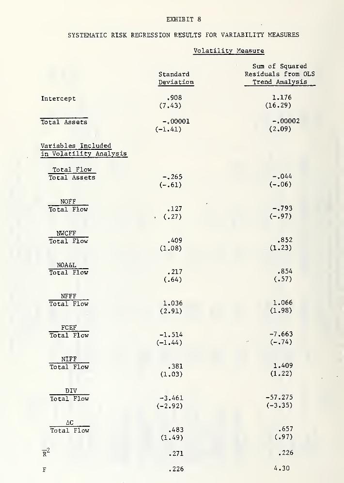
EXHIBIT 8

SYSTEMATIC RISK REGRESSION RESULTS FOR VARIABILITY MEASURES

Volatility Measure

Sum of SquaredResiduals from OLS

Trend AnalysisStandardDeviation

Intercept .908

(7.43)

Total Assets -.00001(-1.41)

Variables Includedin Volatility Analysis

Total FlowTotal Assets -.265

(-.61)

NOFFTotal Flow .127

• (.27)

NWCFFTotal Flow .409

(1.08)

NOA&LTotal Flow .217

(.64)

NFFFTotal Flow 1.036

(2.91)

FCEFTotal Flow -1.514

(-1.44)

NIFFTotal Flow .381

(1.03)

DIVTotal Flow -3.461

(-2.92)

AC

Total Flow .483

(1.49)

r2 .271

F .226

1.176(16.29)

-.00002(2.09)

-.044(-.06)

-.793(-.97)

.852

(1.23)

.854

(.57)

1.066

(1.98)

-7.663(-.74)

1.409(1.22)

-57.275(-3.35)

.657

(.97)

.226

4.30

HECK^AANBINDERY INC.

JUN 95

cash flows and market risk - illinois: ideals home

Documents