Cash Flows and Leverage Adjustments

Michael Faulkender, Mark J. Flannery, Kristine Watson Hankins, and

Jason M. Smith∗

August 12, 2010

Abstract

Recent research has emphasized the impact of transaction costs on firm leverage

adjustments. We show here that a firm’s cash flow realization affects how quickly it

moves toward a leverage target, consistent with the hypothesis that large (positive or

negative) operating cash flows provide an opportunity to adjust leverage at relatively

low marginal cost. Accounting for this fact produces adjustment speeds that are sig-

nificantly faster than previously estimated in the literature. Firms that can spread the

costs of market access across their cash flow needs and their deviation from target ac-

tually adjust very quickly toward their targets. The fact that these speeds do not reach

unity implies that movement toward the target also has a variable cost component. We

analyze how both financial constraints and market timing variables affect adjustments

toward a leverage target.

∗Faulkender is from the Robert H. Smith School of Business, University of Maryland at College Park,Flannery is from the Graduate School of Business, University of Florida, and Hankins and Smith are bothfrom the Gatton College of Business and Economics, University of Kentucky. For helpful comments onpreceding drafts, we thank Vidhan Goyal, Brad Jordan, Mark Leary, Mike Lemmon, Mitchell Petersen, andseminar participants at Oxford University and Iowa State University.

1 Introduction

Do firms have leverage targets? How quickly do they approach these targets? What are the

drivers of the targets? What are the impediments to achieving those targets?

We are not the first to ask these questions. Recent studies include Flannery and Rangan

(2006), Leary and Roberts (2005), Huang and Ritter (2009), and Frank and Goyal (2009)1

Almost all research in this arena concludes that firms do have targets (Welch (2004) being the

obvious exception) but that the speed with which these targets are reached is unexpectedly

slow. This has moved the literature towards a search for the source(s) of adjustment costs.

For example, Fisher, Heinkel, and Zechner (1989) argue that firms will adjust leverage only

if the benefits of doing so more than offset the costs of reducing the firm’s deviation from

target leverage. Altinkilic and Hansen (2000) present estimates of security issuance costs,

and others have modeled the impact of transaction costs on observed leverage patterns (e.g.

Strebulaev (2007), Shivdasani and Stefanescu (2010), and Korajczyk and Levy (2003)).

Leary and Roberts (2005) derive optimal leverage adjustments when transaction costs have

fixed or variable components.

Much of the existing literature implicitly assumes that firms access the capital markets

solely in order to approach their target leverage ratio.2 This clearly is not true. Some firms

raise external funds to finance investment opportunities or to cover operating shortfalls.

Other firms (”cash cows”) routinely generate cash beyond the value of their profitable in-

vestment opportunities and may eventually distribute that cash to stakeholders. Any sort of

capital market access can be used to adjust leverage, if the firm wishes to do so: funds can

be raised by issuing either debt or equity,; excess cash can be distributed by retiring debt,

paying dividends, or repurchasing shares. A firm’s cash flow needs can substantially affect

the cost of making a leverage adjustment, although most of the existing empirical exami-

1In addition, see Lemmon, Roberts, and Zender (2008), Kayhan and Titman (2007), Hennessy, Livdan,and Miranda (2010), Mehrotra, Mikkelson, and Partch (2003), or Jalilvand and Harris (1984).

2In part, this assumption reflects the fact that few researchers estimate capital structure models withendogenous investment decisions. Exceptions include Brennan and Schwartz (1984), Whited and Hennessy(2005), Titman and Tsyplakov (2007), and DeAngelo, DeAngelo, and Whited (Forthcoming).

1

nations assume that firms adjust purely on the basis of their distance from target leverage.

Two stylized examples can illustrate the close connection between operating cash flows and

observed leverage adjustments.

First, consider a firm with a constant target leverage ratio and high costs of accessing

external capital markets. It starts out with leverage below its target (optimal) level and

would enhance value by closing the gap. In one year, its cash flow realization is near zero and

it has few investment opportunities. In the subsequent year, its cash flow falls well below the

amount needed to fund all valuable investment opportunities. If accessing external capital

markets entails transaction costs, this firm is much more likely to adjust its leverage in the

second year. Yet its market access costs have not changed between these two years. Second,

consider two firms, both of which are under-levered and wish to move closer to their leverage

targets. Firm A faces low costs of accessing external markets, but rarely does so because

its operating cash flows are usually sufficient to fund its valuable investment opportunities,

but little more. Adjusting Firm A’s leverage would require a “special” trip to the capital

markets, and the associated costs would be offset only by the benefits of moving closer to

target leverage. Firm B has higher access costs than Firm A, but its operating cash flows

are much more volatile. In some years, Firm B’s investment opportunities are so great

that funding them requires external capital. In other years, Firm B has large excess cash

flows, which it finds optimal to distribute to its stakeholders. Regardless of whether Firm

B is raising or distributing funds, it can simultaneously adjust its leverage at relatively low

marginal cost. We might therefore observe that the firm with higher adjustment costs (Firm

B) nonetheless adjusts its capital structure more frequently than Firm A.

Both of these examples indicate that recognizing multiple reasons for accessing external

capital markets provides an opportunity to identify firms that are particularly likely to

make leverage adjustments if they care about target leverage. In this paper, we model

leverage adjustment speeds in light of firms’ other incentives to access capital markets.

Our econometric specification permits a firm’s cash flow realization affect the (fixed and/or

2

variable) costs of adjusting leverage.

Accounting for a firm’s cash flow realization provides significantly different interpreta-

tions from what has been documented in the literature. The differences in magnitudes are

substantial and demonstrate just how important recognizing the role of cash flow is in esti-

mating the source and magnitude of adjustment costs. For firms with cash flow realizations

near zero, we estimate adjustment speeds in the range of 23% to 26%, similar to what has

been previously found in the literature. However, for firms with cash flows significantly

distant from zero and in excess of their deviation from their leverage target, we find ad-

justment speeds in excess of 50%. This number rises to greater than 70% if the firm is

over-levered. These results are not just statistically significant. The magnitudes of these

estimated parameters indicate that cash flow realizations are a first-order concern for firms

and highlight their importance when testing for cross-sectional and time-series variation in

adjustment costs. The results are remarkably robust to alternative measures of cash flow,

the incorporation of firms’ beginning of period cash position into the cash flow calculation,

and alternative estimates of the firm target leverage levels.

With this specification in place, we then seek to understand the relative importance of

two sources of potential adjustment costs that have been raised in the literature: financial

constraints and market timing. Financially constrained firms may be unable to issue securi-

ties that would move them toward their target leverage ratios, or such securities might simply

be prohibitively expensive. Using various measures to control for financial constraints, we

estimate how they affect the impact of the cash flow realization on leverage adjustment

speeds. Similarly, some have argued that market conditions may alter firms’ perceived costs

and benefits of achieving their target leverage ratio. For instance, an over-levered firm that

considers its shares to be over-valued will see an adjustment toward target leverage via an

equity issuance as low cost. However if that same firm were under-levered, it may choose to

become even more under-levered if it perceives the value of the mis-priced equity to exceed

the marginal value of approaching target leverage. We estimate the variation in adjustment

3

speeds across several indicators of financial market conditions to estimate the economic sig-

nificance of market timing considerations as an explanation for the slow speed of adjustment

previously documented in the literature.

Overall, we show that the effects of financial constraints have nearly an order of magnitude

larger effect on the variation in adjustment speeds across firms relative to the effects of

market timing considerations. These results indicate that the relative accessibility of markets

generates significant variation in the costs firms face when approaching capital structure

adjustments. Although market timing effects do alter capital structure adjustments on the

margin (the effects are statistically significant), the economic magnitudes do not appear

sufficiently sizable to explain slow adjustment speeds.

The paper is organized as follows. Section 2 presents some basic empirical models of cor-

porate leverage, describes data sources, and explains how we compute target leverage ratios

for each firm-year. We illustrate some distinguishing features of our approach in Section 3,

including the importance of distinguishing between under- and over-levered firms’ leverage

adjustments. Section 4 introduces the paper’s major innovation. We explain why operating

cash flows affect a firm’s cost of making leverage adjustments, and modify a standard partial

adjustment model to reflect the interaction between a firm’s cash flow needs and its capital

structure adjustments. The resulting estimated adjustment speeds are substantially larger

than previous estimates in the literature. We analyze the robustness of our results in Section

5. Section 6 then extends the model in Section 4 to test whether financial constraints and

market conditions affect adjustment speeds. We find that adjustment speeds vary plausibly

with both cross-sectional and inter-temporal variables, supporting our partial adjustment

model of capital structure adjustment. The final section summarizes results and discusses

their implications for capital structure theories.

4

2 Basic Leverage Models and Data

A standard partial-adjustment model of firm capital structure estimates a regression of the

form:3

Li,t − Li,t−1 ≡Dt

At

−Dt−1

At−1

= λ(L∗

i,t − Li,t−1

)+ εi,t (1)

where Dt is the firm’s outstanding debt at time t, At is the firm’s outstanding book assets at

time t, Li,t is contemporaneous leverage, Li,t−1 is lagged leverage, and L∗

i,t is the estimated

target leverage ratio, given firm characteristics at t-1. The typical sample firm closes λ

percent (per time period) of the gap between its target leverage and its beginning of period

leverage. This “lambda” value is commonly called the firm’s speed of “adjustment” toward

target.

Note that the specification (1) assumes that a firm’s adjustment starts from the prior

period’s leverage, Li,t−1. Absent any active capital structure adjustments, however, leverage

will change from Li,t−1, when the firm posts its annual income to its equity account. An

active adjustment requires that the firm access capital markets in some way, even if only to

pay dividends. Likewise, only active adjustments entail transaction costs, so therefore, tests

of target adjustment models should focus on active adjustments. We revise (1) to separate

a firm’s leverage change into a passive, mechanical component and an active adjustment:

Li,t − Lpi,t−1

= γ(L∗

i,t − Lpi,t−1

)+ εi,t (2)

where

Lpi,t−1

≡Dt−1

At−1 + NIt

and NIt is equal to net income during the year ending at time t. Leverage at t would be Lpi,t−1

if the firm engages in no net capital market activities. The left hand side of (2) therefore

equals the firm’s active “adjustment” toward target capital structure change.

3See Flannery and Rangan (2006), Lemmon, Roberts, and Zender (2008), and Huang and Ritter (2009).

5

We follow previous researchers in studying leverage decisions for all Compustat firms with

the exception of financial firms (SIC 6000-6999) and utilities (SIC 4900-4999), for the time

period 1965-2006. Using the combination of annual Compustat and CRSP data, we estimate

a partial adjustment model that specifies the target capital ratio as depending on the firm

characteristics employed by Flannery and Rangan (2006). Although previous studies have

used both market-valued and book-valued equity measures, we concentrate on book leverage

because decomposing the active and passive pieces is more straightforward.4 To reduce the

effect of outliers, all ratios are winsorized at the first and ninety-ninth percentiles. Table 1

defines all variables and presents summary statistics.

Both regressions (1) and (2) rely on an estimated target leverage, L∗

i,t. The most chal-

lenging aspect of estimating either regression is constructing an estimate of the firm’s target

leverage. Many recent papers estimate target leverage concurrently with the speed of ad-

justment toward target, as in (2). For reasons that will become more clear below in Section

6.1, we estimate a target first; then (1) or (2) can be estimated by OLS with bootstrapped

standard errors.

The recent literature on firm leverage models concludes that allowing for incomplete

adjustment is important, and that firm fixed effects are required to capture unobserved firm-

level heterogeneity (Flannery and Rangan (2006), Lemmon, Roberts, and Zender (2008)).

We begin by estimating a partial-adjustment model of leverage for all sample firms, using

the restriction that L∗

i,t = βXi,t−1:

Li,t = γβXi,t−1 + (1 − γ)Lt,t−1 + εi,t (3)

where β is a coefficient vector to be estimated concurrently with γ and Xi,t−1 includes:

a firm fixed effect,

EBIT TA = (Income before Extraordinary Items + Interest Expense + Income Taxes) /

4Substituting market for book valued leverage measures yields similar results, as suggested by the firsttwo columns of Table 2.

6

Total Assets,

MB = ((Book Liabilities plus Market Value of Equity) / Total Assets,

DEP TA = Depreciation and Amortization / Total Assets,

LnTA = ln (Total Assets deflated by the consumer price index to 1983 -

dollars),

FA TA = Net property, plant and equipment / Total Assets,

R&D TA = Research and Development Expense / Total Assets,

R&D Dum = 1 if Research and Development Expense > 0, else zero, and

Ind MedianLeverage = Median Debt Ratio for the firm’s Fama and French (1997)

industry. This sort of dynamic panel model entails some important estimation issues (Nickell

(1981), Baltagi (2008)), which several econometric techniques have been designed to address.

Flannery and Hankins (2010) conclude that the Blundell and Bond’s (1998) system GMM

estimation method generally provides adequate estimates. We estimate (3) via Blundell

and Bond’s system GMM and compute L∗

i,t. Equation (1) and (2) can then be estimated

using OLS, with bootstrapped standard errors to account for the generated regressor (Pagan

(1984)).

Estimation results for (3) correspond closely to estimates presented previously in the

literature for both market and book valued leverage measures, and for brevity are not pre-

sented.5

3 Initial Estimation Results

Table 2 reports the results from estimating the basic regression models. The first two columns

report estimates for (1), using book- and market- valued leverage, respectively. Book-valued

(market-valued) leverage yields an annual adjustment speed of 21.9% (22.3%). These results

closely resemble previous estimated adjustment speeds (e.g. Lemmon, Roberts, and Zender

5Targets estimated from the entire sample period (1965-2006) are used in all our reported results exceptTable 6 when rating data is available from 1986-2006. We also included additional variables to explain targetleverage in some instances, but our results are not sensitive to such changes. See Section 5 below.

7

(2008)). The implied adjustment speeds are very similar between market and book values,

consistent with most of the existing literature. The third column of Table 2 estimates

a baseline adjustment speed using our measure of active leverage in equation (2). The

estimated adjustment speed rises to 40.2% for this measure of active leverage adjustment.

One reason for this increase may be that the median firm has positive net income and

is under-levered. Absent active leverage adjustments the median firm tends to become

even more under-levered, so when a firm does actively adjust its capital structure, our

alternative measure of “starting” leverage gives the firm some credit toward undoing the

effect of positive net income. This portion of adjustment is not captured in specification

(1). Given our interest in how cash flows affect (costly) active leverage adjustments and the

empirical effect of using Lpi,t−1

as the firm’s starting point in adjusting leverage, we continue

with it throughout the rest of the paper.

Our second refinement to the basic specification (1) eliminates the symmetry between

under- and over-levered firms. Previous researchers have generally assumed that all firms

adjust their leverage ratios at the same rate, with DeAngelo et al. (Forthcoming) being

one notable exception. However, one can readily imagine reasons why optimal adjustments

vary asymmetrically across firms.6 Even if adjustment costs were equal for under- and over-

levered firms, the benefits may be asymmetrical. Under-levered firms forego tax benefits of

leverage and have little concern with financial distress costs. Yet potential financial distress

costs loom quite large for over-levered firms. There is no theoretical reason why the net

tax benefit minus expected financial distress costs should be symmetrical around the firm’s

optimal leverage ratio, and therefore no reason to specify that the absolute distance from

target leverage fully captures a firm’s incentives to adjust.

The left half of Table 3 reports the results of estimating the base model (2) separately

for over-levered and under-levered firms. The estimated adjustment speeds are strikingly

6For example, Korajczyk and Levy (2003) provide evidence that the leverage adjustments made byconstrained and unconstrained firms differ.

8

different: 29.8% per year for under-levered firms vs. 56.4% for over-levered firms.7 On its

face, this result suggests that over-levered firms have either greater benefits or lower costs of

adjusting toward their target leverage ratios.

Given the significant differences in adjustment speeds between under- and over- levered

firms, all of our subsequent specifications will be estimated separately for these two sub-

samples. As an added benefit, we shall see in Section 5 that estimating separate models for

over- and under-levered firms aids our interpretation of how market timing variables affect

convergence to target leverage.

4 The Effect of Cash Flow on Capital Market Adjust-

ment Costs

Our third - and most important – modification to the standard partial adjustment model

(1) recognizes that a firm’s operating cash flow (CF) may affect the cost of making lever-

age adjustments. CF has two potential effects on leverage adjustment. First, CF needs

accommodated in the market create a low-cost opportunity to adjust leverage. If a firm

needs to raise external funds and has a leverage target, it can choose to issue debt or equity

according to whether it is under- or over-levered. Likewise, a firm with high positive cash

flow will tend to distribute funds to investors, but it can affect leverage by choosing to pay

down either debt or equity. The sign of cash flow doesn’t matter, just its absolute value.

Second, if firms confront a fixed cost of accessing capital markets, they are more likely to

make leverage adjustments when part of the fixed market access cost is borne by the firm’s

need to accommodate its cash flow imbalances.

7A similar result is reported by Byoun (2009), whose regression specification examines changes in a firm’soutstanding debt under various cash flow conditions. Our estimates differ from Byoun’s along two importantdimensions. First, his specification ignores explicit changes in outstanding equity, and thus cannot detectchanges in leverage, but only changes in the “numerator”, outstanding debt. Second, our specifications willuse continuous variables for cash flow and deviation from target leverage to make inferences about variableadjustment costs, while Byoun uses a dummy variable to indicate whether the firm’s cash flow is positive ornegative.

9

We define a firm’s operating cash flow (or financing deficit) as:

CFi,t =OIBDi,t − Ti,t − Inti,t − Industry CapExt

Ai,t−1

(4)

where

OIBDi,t is operating income before depreciation,

Ti,t is the total taxes allocated on the income statement,

Inti,t is the interest paid,

Industry CapExt is the mean value of capital expenditures in year t (deflated by lagged

book assets) for all Compustat firms in firm i’s Fama-French (1997) industry, and

Ai,t−1 is the value of total assets for the fiscal year ending at t-1.

The first three terms in (4) are included in standard measures of a firm’s financing deficit,

beginning with Shyam-Sunder and Myers (1999). Some prior researchers have subtracted out

the firm’s actual capital expenditures to yield its external financing requirement. However,

we proxy for the firm’s investment opportunity set with Industry CapExt. A firm’s observed

expenditures reflect both the firm’s investment opportunity set and its decision to access

financial markets. The latter could be correlated with a firm’s leverage gap, leading us to

employ Industry CapExt as an instrument.

We expect that firms with high absolute CF are more likely to make leverage adjust-

ments, if leverage targets mean anything to them. To a first approximation, the CF ’s sign

does not matter. Consider first a firm for which large investment opportunities generate a

negative CF . If the NPV of these investment opportunities exceeds the cost of accessing

financial markets, the firm will raise external funds and any transactions related to leverage

adjustment can be made “free” of that fixed access cost. Even if the investment opportunities

are insufficient to warrant market access on their own, the combination of investment and

leverage benefits might justify the cost of capital market access. Analogously, a firm with

a large positive CF will consider distributing excess funds to the market by repurchasing

10

either shares or debt, according to its leverage gap.

We can learn something about the costs of adjusting capital structure by comparing the

size of a firm’s CFi,t to its scaled deviation from target leverage:

Devi,t = L∗

i,t − Lpi,t−1

. (5)

A firm whose |Dev| exceeds its |CF | can make a leverage adjustment up to |CF | at low

cost because the market access costs are shared between the benefits of approaching target

capital structure and the funding/distribution of realized cash flow. However, a leverage gap

beyond |CF | will be closed only if the marginal cost of additional capital market transactions

is sufficiently low. Unless variable cost is zero, we expect that the firm’s adjustment speed

toward target will be faster for |Dev| up to |CF | than beyond that point.

Next, consider a firm whose |CF | exceeds |Dev|. This firm has sufficient funding needs (or

excess cash to return to stakeholders) to reach its leverage target by choosing appropriately

between debt and equity transactions. In other words, the firm can simultaneously close

its leverage gap and resolve its cash flow needs. We therefore anticipate that firms with

such large (absolute) cash flows will make large movements to close |Dev|. In the absence

of variable adjustment costs, this coefficient might approach unity. However, for the |CF |

beyond the initial |Dev| the firm’s debt-equity choice should preserve the (attained) target

leverage, and hence we expect no change in leverage from this sort of “excess” cash flow.

This intuitive discussion has divided CF and Dev into four segments:

ExcessDev ≡ (|Dev| − |CF |) ∗ DevLarger

Overlap, |Dev| > |CF | ≡ |CF | ∗ DevLarger

Overlap, |CF | > |Dev| ≡ |Dev| ∗ (1 − DevLarger)

ExcessCF ≡ (|CF | − |Dev|)∗(1−DevLarger) where DevLarger = 1 if |Dev| > |CF |,

otherwise = 0. The first three variables decompose leverage deviation into the part that

exceeds |CF | and two parts that “overlap” |CF |. The fourth variable, “ExcessCF” measures

11

cash flow needs beyond those required to close the leverage deviation completely. If these

segments involve different costs of adjusting leverage, we should generalize (2) into a modified

partial adjustment model:

Li,t − Lpi,t−1

={

[γ1 (|Dev| − |CF |) + γ2|CF |] ∗ DevLarger+ (6)

[γ3|Dev| + γ4 (|CF | − |Dev|)] ∗ (1 − DevLarger)}∗ Sign + εi,t

where Sign = 1 if the firm is over-levered and = −1 otherwise.8 Equation (6) is designed

to identify leverage adjustments that are relatively inexpensive to undertake. γ2 and γ3

measure the firm’s propensity to adjust leverage when its cash flow situation makes these

adjustments easiest to undertake.9 Assuming that firms wish to move toward their target

leverage ratios, γ2 and γ3 should be quite large:

• When the |Dev| exceeds the |CF |, all of |CF | is available to adjust leverage toward

target.

• When |CF | exceeds |Dev|, the firm’s cash flow needs permit it to attain target leverage.

With zero variable transaction costs, γ1 should equal γ2: once any fixed cost of accessing

the external market has been incurred, the firm should close |Dev| equally with CF-related

funds or with transactions aimed solely at closing |Dev|. However, positive variable costs

will leave γ1 < γ2 because transactions aimed exclusively at closing |Dev| have more benefits.

γ4 should also be small: a firm with Excess |CF | can attain its target leverage in the course

of fulfilling its CF needs, so further transactions should leave leverage undisturbed. In

summary, we hypothesize that γ3 ≈ γ2 > γ1 > γ4.

As an example, consider a firm that is under-levered by 5% of its (lagged) total assets

and has a cash flow deficit equal to 8% of its lagged total assets. The partial adjustment

8This sign adjustment accounts for the fact that the dependent variable is signed, while the explanatoryvariables are all positive by construction.

9Firms with DevLarger = 0 will tend to be closer to their target leverage than the firms withDevLarger = 1. Therefore, we (weakly) anticipate that γ3 > γ2.

12

model predicts that the first five percentage points of the cash flow deficit (corresponding to

the value of the γ3 variable in (6)) will be raised in the form of debt, which would generate

γ3 = 1. What about the remaining 3% of the cash flow deficit? Assuming that the firm

finds it more costly to liquidate assets than raise capital and does not have sufficient internal

liquidity, it would raise the additional 3% of assets according to its target leverage ratio.

For instance, if the firm’s target leverage ratio were 40% and the initial debt issuance (the

5%) has attained that leverage, 1.2 percentage points of the remaining 3% financing need

would be raised as debt and the other 1.8 percentage points raised as equity. As a result, we

hypothesize that this marginal CF will leave leverage unaffected on average. That is, the

coefficient on γ4 will be near zero. Now reverse the numbers in our example: make the firm

under-levered by 8% of its (lagged) total assets, with a cash flow deficit equal to 5% of its

lagged total assets. The firm is again predicted to close the first 5% of the leverage deficit

with a debt issuance (γ2 = 1). What about the remaining 3% of Dev? With a high marginal

(variable) transaction cost, the firm will do nothing to close this part of the deviation. On

the other hand, with sufficiently low variable costs, it would raise the additional 3% of assets

in the form of debt (given that the fixed access cost has already been paid). The higher the

variable cost, the closer to zero γ1 is predicted to be.

Estimation results for (6) are presented in the right half of Table 3, separately for under-

levered and over- levered firms. Our hypothesized rank ordering of estimated γ coefficients

holds in both sub-samples. When cash flows are large (in absolute value) the leverage

adjustments (γ2, γ3) are also large. The typical over-levered firm devotes between 69%

and 90% of its cash flow realization to capital transactions that close the gap between

actual and target leverage, compared to 27%-52% for under-levered firms. As in Table 3

the benefits of removing excess leverage apparently exceed the benefits of moving toward

target leverage from below. Note that leverage adjustments are significantly smaller for the

ExcessDev, which suggests that capital market transactions involve at least some variable

transaction costs. Finally, the insignificant coefficients on ExcessCF indicate that firms make

13

no systematic leverage changes once they have eliminated their deviation from target.

Table 4 refines the CF variables’ definition (4) to reflect a firm’s ability to buffer the

effects of volatile cash flows by holding liquid “cash” assets. The cash flow definition in (4)

ignores accumulated cash balances, yet such balances can separate cash flow realizations from

the need to access external capital markets (Opler, Pinkowitz, Stulz, and Williamson (1999),

Almeida, Campello, and Weisbach (2004)). Table 4 refines the CF variables’ definition (4)

to reflect a firm’s ability to buffer the effects of volatile cash flows by holding liquid “cash”

assets. We explore two specifications for incorporation of cash balances by revisiting the

definition of CF (4) and re-estimating (6). First the cash position is added to the numerator

of (4). Estimation results in the first and third columns of Table 4 reveal some changes in

estimated adjustment speeds, but the main results remain unchanged from the right half

of Table 3: firms close a significant portion of their target leverage differential when the

adjustment cost is shared with addressing the cash flow realization. The adjustment speed is

considerably smaller when the adjustment cost is only offset by the benefits from approaching

target leverage: the hypothesis that γ1 = γ2 is rejected. Another way to incorporate cash

balances into our measure of CF is to recognize some of a firm’s cash may be required

for operating liquidity. We therefore replace the firm’s beginning-of-period cash position

(in (4)) with an estimate of its excess cash position, measured as the firm’s beginning-of-

period of cash less the beginning-of-period Fama French (1997) industry average cash level,

normalized by size). The results in columns (2) and (4) of Table 4 are nearly identical to

those found from using the firm’s total cash position.

We conclude two things from Table 4. First, leverage adjustment costs are important in

determining how much firms adjust. Otherwise, cash flow realizations would not have a first-

order effect on the extent of leverage adjustment documented above. Second, adjustment

costs appear to have at least a variable component. If the cost were entirely fixed, once

the firm absorbs the fixed cost associated with addressing its cash flow realization, it should

adjust all the way to its target. This would generate γ1 and γ2 coefficients that do not

14

significantly differ from each other.

5 Robustness

Our results are robust to alternative measures of target leverage and to variations of our

cash flow measures. Because Korajczyk and Levy (2003) find that leverage levels vary with

macroeconomic conditions, we re-estimate our target leverage ratios with year dummies to

allow time series variation at the macroeconomic level to alter firms target leverage positions

for the corresponding fiscal year. Using these alternative targets, we re-estimate equation

(6) and report the results in the two columns of Table 5 labeled “I”. Comparing the results

to those found in the right half of Table 3, allowing leverage to change with movements in

the macroeconomy does not alter the effect of cash flow realizations on leverage adjustment

speeds.

We make three further adjustments to our definition of the firm’s cash flow realization

(equation (4)), contained in columns (II), (III), and (IV) respectively of Table 5. First, we

subtract the change in working capital, recognizing that short term assets and liabilities can

serve as alternative sources and uses of cash. Second, we subtract the cash dividends paid

in the previous fiscal year, on the assumption that firms view their dividend stream as a

committed use of cash similar to a required interest payment to debt holders (Graham and

Harvey (2001)). Third, if firms have debt maturing in the current fiscal year, they will need to

refinance that maturing debt unless their operating cash flow is sufficiently positive. Tapping

external capital markets to refinance existing debt will also lower the cost a firm incurs from

approaching target leverage. Therefore, we subtract short-term debt (Compustat data 34

- debt in current liabilities) to arrive at our third alternative measure of cash flow. The

results are extremely robust and consistent with our prior results. Very rapid adjustment

speeds on the two Overlap variables indicate that CF needs substantially reduce the cost of

adjusting leverage. The smaller coefficients on ExcessDev are consistent with the hypothesis

15

that leverage adjustment costs include a variable component.10

Finally, we estimated (6) as part of an endogenous choice (Heckman) model, in which

the other equation is a probit model explaining which firms “accessed” capital markets in

the form of sufficiently large changes in their outstanding debt and/or equity.11 We then

estimate (6) only for firms that accessed the market, and include the inverse Mills ratio as an

additional explanatory variable. The first-stage (probit) regression indicates that firms are

more likely to access external capital markets when they have larger |CF | or larger |Dev|,

consistent with the existence of a fixed access cost. The second stage (regression model (6))

results were very similar to those reported in Table 3.

6 Financial Constraints and Market Timing

A growing literature suggests that the ability to tap capital markets varies across firms.

For example, Faulkender and Petersen (2006) provide evidence that access to the public

bond market enables a firm to be more levered, particularly when there are shocks to credit

markets (Leary (2009)). We now test the validity of our basic model by examining how firm

and financial market characteristics affect adjustment speeds. A growing literature draws the

distinction between financially “constrained” and “unconstrained” firms (e.g. Korajczyk and

Levy (2003)). As is customary in the literature, we have included two measures of financial

constraints in estimating target leverage (size and rating). But financial constraints could

also affect a firm’s ability to adjust toward its target leverage. Indeed, one might define

“better” capital market access as lower costs of moving toward target leverage. We therefore

wish to investigate whether firms that are less likely to be constrained (those that are larger,

pay dividends, or have access to public bond markets) adjust more rapidly.

Similarly, some authors conclude that transitory market conditions influence security

10In untabulated results, we simultaneously make all three adjustments and the results mirror thosereported here. These results are available upon request.

11As suggested by Strebulaev (2007), we hereby estimate an adjustment model only for firms that are mostlikely to have adjusted. This approach resembles Leary and Roberts (2005), who utilize a hazard functionto characterize capital market accessing decisions.

16

choices and that these influences permanently affect a firm’s equilibrium capital structure

(e.g. Baker and Wurgler (2002) and Korajczyk and Levy (2003)). We argue that it is also

plausible that market timing considerations affect a firm’s short-term incentives to close

a leverage gap.12 To illustrate how market timing forces might affect adjustment speed,

consider an over-levered firm that may retire some of its outstanding debt. This inclination

would likely be reinforced if corporate bond yields were temporarily high (making debt prices

low), but it might be delayed if yields were considered temporarily low. So this firm would

be more likely to engage in a greater adjustment towards target leverage as bond yields

rise.13 Another over-levered firm might be planning to issue shares. Bond rates may be less

relevant for this firm, but it would be particularly anxious to issue equity when its share price

seems to be temporarily high. The value of this mis-pricing opportunity will affect how much

to adjust contemporaneously, and the effect on capital structure will persist until the firm

finds it worthwhile to again modify their capital structure. We therefore hypothesize that

capital structure adjustment speeds should respond to some of the market timing variables

previously identified in the literature as affecting leverage levels.

6.1 Modifications to the Partial Adjustment Model

Combining a state-dependent adjustment speed with a firm-specific target involves some

important econometric adaptations. One might initially consider estimating a separate re-

gression like (6) for the time periods with high vs. low values for the variable(s) affecting

adjustment speed. However, multiple estimations of (6) would fail to impose a consistent

model of target leverage (including the firm’s fixed effect) across those specifications.

We can generalize our basic dynamic panel model by specifying that the ith firm’s ad-

12Korajczyk and Levy (2003) permit market and firm conditions to affect both the firm’s estimated targetand its decision about whether to issue debt or equity (conditional on some issuance). They would say thata firm’s target leverage varies with macro variables. Our results are based on targets calculated without yeardummies. However, they are robust to the inclusion of year dummies, which should subsume most of theintertemporal variations in macroeconomic conditions.

13For example, Graham and Harvey (2001) find survey evidence that CFOs try to issue bonds when interestrates are relatively low.

17

justment speed at time t depends on a variable of interest, Zk,t

Li,t − Lpi,t−1

= (γ0 + γ1kZk,t)(L∗

i,t − Lpi,t−1

)(7)

As above, proxies for the target values L∗

i,t−1are generated from (3). We examine both

“financial constraint” variables and “market timing” variables (the Zi,t).

1. Financial constraints are likely to reflect cross-sectional variation in the costs and

benefits of adjusting firm leverage. Therefore, we should see that for the same deviation

from target leverage and the same cash flow realization, highly constrained and less

constrained firms adjust their capital structure differently. We use three financial

constraint proxies:

• Size = ln(Basseti,t−1)

• Divs = 1 if the firm paid dividends in year t-1, 0 otherwise

• Rated = 1 if the firm has a bond rating, 0 otherwise

Following Faulkender and Wang (2006) and Almeida, Campello, and Weisbach (2004)

among others, a firm’s ability to access capital markets is likely to vary with size

(ln(Basset)). To the extent that access costs have a fixed component, a larger firm will

find it worthwhile to incur that fixed cost more often than a smaller firm. Dividend

payers are thought to have relatively unconstrained access to capital markets; if not,

they would retain the funds they generate rather than pay dividends. Firms that are

rated should have relatively lower costs of accessing financial markets. We examine

differences in capital structure adjustment speeds for all three measures.

2. Market timing variables measure financial market conditions that may affect a firm’s

interest in accessing the capital markets at a specific time. We use three market timing

proxies:

• Baa = average Baa yield for the year between t-1 and t

18

• IndMB = Average Industry MB

• MBDiff = Firm MB - IndMB

A temporarily high Baa rate might discourage firms from issuing new debt (Graham (1996)),

which may reduce leverage adjustment speeds for under-levered firms. However, the same

high Baa rate may encourage adjustment by firms wishing to retire outstanding debt (at

a discount). Likewise, the firm’s market-to-book ratio relative to that of the industry may

affect firms’ interest in accessing capital markets (consistent with Baker and Wurgler (2002),

among others), but the effect would differ according to whether the firm was planning to

issue or to redeem shares.

We estimate the following regression specification separately for over- and under- levered

firms:

Li,t − Lpi,t−1

=3∑

k=1

{(γ1 + γ1kZk,t) (|Dev| − |CF |) ∗ DevLarger+

(γ2 + γ2kZk,t) ∗ |CF | ∗ DevLarger+

(γ3 + γ3kZk,t) ∗ |Dev| ∗ (1 − DevLarger)+

(γ4 + γ4kZk,t) (|CF | − |Dev|) ∗ (1 − DevLarger)}∗ Sign + εi,t (8)

To ease economic interpretation, the four continuous variables (size, Baa rate , MB Diff ,

and IndMB) have been normalized to have mean zero and standard deviation of one. This

permits easy calculations of the effects of changes in the Z values on adjustment speed. Table

6 reports estimation results for the three financial constraint interactions and Table 7 reports

analogous results for the three market timing interactions.

19

6.2 Financial Constraints Results

Under-levered firms are described in the first four columns of Table (6) and over-levered

firms are in the last four columns.14

Consider first the under-levered firms. The “base” estimates correspond to a firm with

Div = 0, Rated = 0, and (because the variable has been normalized) Size at the the sample

mean. We find that larger firms adjust less quickly than smaller ones, despite the fact that

(theoretically) they should be less sensitive to fixed transaction costs. It thus appears that

larger, under-levered firms enjoy lower benefits of increasing leverage. However, the other two

indicators of financial constraint carry large, positive coefficients, implying faster adjustment

by less constrained firms. A bond rating more than doubles the adjustment speed associated

with an overlap between |Dev| and |CF |. (See rows (b) and (c).) It also increases by nearly

one-half the speed with which ExcessDev is closed (row (a)). As expected, Rated has no

effect on ExcessCF adjustments in row (d), because these CF are relevant only after the firm

has attained its target debt ratio. The Div variables’ coefficients similarly indicate faster

adjustment for less constrained firms, but the estimated differences are much more modest.

The over-levered subsample results (in the right half of Table 6) again indicate much

faster Base adjustment speeds than characterize the under-levered firms. We see again that

larger firms adjust less quickly, although the effects are somewhat smaller than for under-

levered firms. And we see that firms with better access to financing (Div = 1, Rated = 1)

adjust statistically and economically less rapidly. For example, firms with overlapping cash

flow and deviation (rows (b) and (c)) adjust between 75% and 87.8% if they do not pay

any dividends, are average sized, and have no rating. In other words, constrained firms act

quickly to eliminate excess leverage, while less constrained firms move much less urgently.

For example, a dividend-payer that is one standard deviation above the mean size and has a

14Because rating information is available only after 1985, the regressions in Table 6 include dates from1986-2006. The results in Table 6 use target proxies computed by estimating (3) over the 1986-2006 sampleperiod. Very similar results result if we utilize target estimates based on the full sample period (1965-2006).Moreover, our results in Tables 6 and 7 are qualitatively unaffected by adding the financial constraint ormarket timing variables to determinants of target leverage in (3).

20

rating adjusts toward target leverage at an annual rate between 35.9% (0.878 - 0.139 - 0.080

- 0.300) and 16.3% (0.750 - 0.287 -0.037 - 0.263). In other words, better financial market

access reduces a firm’s concern about excessive leverage.

Overall, financial constraints significantly change the speed of adjustment toward target

leverage in highly asymmetrical fashion. Constrained firms adjust more slowly (than uncon-

strained firms) when they are under-levered, but more quickly when they are over-levered.

In fact, the estimated effect of financial constraints is sufficient to reverse the un-conditional

estimated speeds in the right half of Table 3. In the simple model (6), over-levered firms

adjust more quickly than under-levered ones, regardless of their |Dev| and |CF |. However,

for a mean-sized firm with no rating and paying no dividends, adjustment is faster when

under-levered than over-levered, according to the results in Table 6. These results indi-

cate the importance of recognizing financial constraints when studying capital adjustments,

and re-emphasize the value of estimating differential adjustment processes for under- vs.

over-levered firms in a sample.

6.3 Market Timing Results

We start our examination of the role of market timing with the under-levered firms in the

first four columns of Table 7. These firms should be issuing debt or retiring equity to close

their leverage gaps. The Base case estimates in the first column of Table 7 correspond closely

to those in the right half of Table 3. Consistent with our hypothesis, a higher interest rate

environment and higher equity valuations decrease the speed with which under-levered firms

will adjust their leverage ratios. However the magnitudes of the change in adjustment speed

are considerably smaller than the results we estimated for the effects of financial constraints.

A decrease in the Baa rate of one standard deviation increases the adjustment speed for

firms with ample cash flow by (row (c)) 11.8%, from 35.7% to 47.5% (35.7% -1*(-11.8%)).

For firms with insufficient cash flow to close their leverage gap (row (b)), the increase in

adjustment speed resulting from a one standard deviation decrease in the BAA rate is 2.0%,

21

from 27.1% to 29.1%. Similarly, higher industry valuations decrease the adjustment speed

of the firm needing to raise its leverage, but these magnitudes are small.

The latter four columns of Table 7 report results for over-levered firms, which will be

retiring debt or issuing shares to close their leverage gaps. For these firms, the effect of

higher interest rates is limited, but higher equity valuations should make it more enticing to

adjust toward target leverage. When industry and firm valuations are high (one standard

deviation above the mean respectively), the speed of adjustment increases from 80.5% to

90.8% (0.805 + 0.016 + 0.087) when cash flow is insufficient to cover the leverage deficit

and from 61.1% to 73.0% (0.611 + 0.020 + 0.099) when cash flow is sufficient to enable an

over-levered firm to completely close its leverage gap (row (c)). These percentages are large

in magnitude and the differences arising from variation in market valuations are statistically

and economically significant. It also makes sense that firms that will primarily engage in

equity increasing transactions are more sensitive to equity valuations than to debt market

measures when determining the portion of their leverage gap to close.

In sum, the results in Table 7 mostly provide intuitive results about the impact of market

conditions on adjustment speeds. Under-levered firms move less quickly toward higher target

leverage levels when interest rates are high. Over-levered firms appear to increase their speed

of adjustment significantly due to higher equity valuations. These results are consistent with

market conditions altering the cost of capital structure adjustment at least temporarily.

7 Summary and Conclusion

Most previous evaluations of corporate capital structure have estimated a single regression

model for all firms, yielding some relatively low estimates of how keen firms are to attain

their target leverage ratios. The infrequent adjustments toward target may reflect a flat valu-

ation function, or the presence of fixed and variable adjustment costs as suggested by Fisher,

Heinkel, and Zechner (1989), Leary and Roberts (2005), and Strebulaev (2007). With sub-

22

stantial costs of accessing capital markets, firms will optimally adjust their capital structures

only when the benefits of adjustment are high or the costs of adjustment are particularly

low. Because cash flow affects a firm’s willingness to interact with capital markets - either to

raise new funds for investment or to return excess cash to stakeholders - internal cash flow

importantly influences the endogenous decision to adjust leverage.

Our results demonstrate that firms with large (positive or negative) operating cash flow

make more aggressive changes in their capital ratios. Consistent with the hypothesis that

the cost of accessing external capital markets importantly affects observed leverage, firms

with high absolute cash flows and high absolute leverage deviations make larger capital

structure adjustments than firms with similar leverage deviations but cash flow realizations

near zero. This result suggests that leverage adjustments are more likely to be made when

adjustment costs are “shared” with transactions related to the firm’s operating cash flows.

This is particularly true of over-levered firms, which close roughly 80% of their leverage

gap when they are transacting for cash flow purposes. Under-levered firms generally close

about 39% of their leverage gaps, suggesting that the benefits of increasing leverage may be

smaller than the benefits of decreasing it. This asymmetry between over- and under-levered

firms reflects general differences that should be taken into account for any empirical study

of corporate leverage.

We find that financial constraints affect the speed with which firms adjust toward target

leverage ratios. Firms that pay dividends or have a credit rating adjust substantially faster

than constrained firms when they are under-levered, and relatively slower when they are

over-levered. Likewise, larger firms adjust excess leverage more slowly, consistent with the

costs of excess leverage being smaller for larger firms. We also examined the analogous effects

of market variables on adjustment. Under-levered firms, which should retire equity, close less

of their leverage gap when share prices are high (relative to book). Analogously, over-levered

firms close substantially more of their leverage gaps when share prices are high. However,

these effects are much less important than the measured effect of financial constraints on

23

firm adjustment speeds.

Overall, our empirical results are consistent with the trade-off hypothesis of capital struc-

ture: firms have targets, and wish to return to those targets when costs make it optimal

to do so. Partial adjustment models yield theoretically sensible results about how a firm’s

characteristics and market conditions affect observed leverage adjustments. However, the

benefits and costs of adjustment vary with the sign of the firm’s leverage gap (over-levered

firms generally adjust more quickly), its access to capital markets, and some elements of

market conditions. Further research should continue to investigate the underlying deter-

minants of adjustment costs and benefits across different sorts of firms, incorporating the

potentially compounding effects of cash flow realizations and the differences between over-

and under-levered firms.

24

References

Almeida, H., M. Campello, and M. Weisbach, 2004, The cash flow sensitivity of cash, Journal

of Finance 59, 1777–1804.

Altinkilic, Oya, and Robert S. Hansen, 2000, Are there economies of scale in underwriting

fees? evidence of rising extrenal costs., Review of Financial Studies 13, 191–218.

Baker, M., and J. Wurgler, 2002, Market timing and capital structure, Journal of Finance

57, 1–32.

Baltagi, Badi H., 2008, Econometric Analysis of Panel Data (John Wiley and Sons).

Blundell, Richard, and Stephen Bond, 1998, Initial conditions and moment restrictions in

dynamic panel data models, Journal of Econometrics 87, 115–143.

Brennan, Michael, and Eduardo Schwartz, 1984, Optimal financial policy and firm valuation,

Journal of Finance 3, 593–607.

Byoun, Soku, 2009, How and when do firms adjust their capital structure toward targets?,

Journal of Finance 63, 3069–3096.

DeAngelo, Harry, Linda DeAngelo, and Toni Whited, Forthcoming, Capital structure dy-

namics and transitory debt, Journal of Financial Economics pp. 1–59.

Fama, Eugene, and Kenneth French, 1997, Industry costs of equity, Journal of Financial

Economics 43, 153–193.

Faulkender, M., and M. Petersen, 2006, Does the source of capital affect capital structure?,

Review of Financial Studies 19, 45–79.

Faulkender, M., and R. Wang, 2006, Corporate financial policy and the value of cash, Journal

of Finance 60, 931–962.

25

Fisher, Edwin O., Robert Heinkel, and Josef Zechner, 1989, Dynamic capital structure choice:

theory and tests, Journal of Finance 44, 19–40.

Flannery, Mark, and Kristine W. Hankins, 2010, Estimating dynamic panels in corporate

finance, Working Paper.

Flannery, Mark, and Kasturi Rangan, 2006, Partial adjustment toward target capital struc-

tures, Journal of Financial Economics 79, 469–506.

Frank, Murray, and Vidhan Goyal, 2009, Capital structure decisions: Which factors are

reliably important?, Financial Management 38, 1–37.

Graham, John, 1996, Debt and the marginal tax rate, Journal of Financial Economics 41,

41–73.

Graham, John R., and Campbell Harvey, 2001, The theory and practice of corporate finance:

Evidence from the field, Journal of Financial Economics 60, 187–243.

Hennessy, Christopher A., Dmitry Livdan, and Bruno Miranda, 2010, Repeated signaling

and firm dynamics, Review of Financial Studies 23, 1981–2023.

Huang, Rongbing, and Jay Ritter, 2009, Testing theories of capital structure and estimating

the speed of adjustment, Journal of Financial and Quantitative Analysis 44, 237–271.

Jalilvand, Abolhassan, and Robert S. Harris, 1984, Corporate behavior in adjusting to capital

structure and dividend targets: An econometric study, Journal of Finance 39, 127–145.

Kayhan, Ayla, and Sheridan Titman, 2007, Firms’ histories and their capital structures,

Journal of Financial Economics pp. 1–32.

Korajczyk, Robert A., and Amnon Levy, 2003, Capital structure choice: macroeconomic

conditions and financial constraints, Journal of Financial Economics 68, 75–109.

26

Leary, Mark, 2009, Bank loan supply, lender choice, and corporate capital structure, Journal

of Finance 64, 1143–1185.

, and Michael R. Roberts, 2005, Do firms rebalance their capital structures?, Journal

of Finance 60, 2575–2619.

Lemmon, Michael, Michael Roberts, and Jamie Zender, 2008, Back to the beginning: Per-

sistence and the cross-section of corporate capital structure, Journal of Finance 60.

Mehrotra, Vikas, Wayne Mikkelson, and Megan Partch, 2003, The design of financial policies

in corporate spin-offs, Review of Financial Studies 16, 1359–1388.

Nickell, Stephen, 1981, Biases in dynamic models with fixed effects, Econometrica 49, 1417–

1426.

Opler, Tim, Lee Pinkowitz, Rene Stulz, and Rohan Williamson, 1999, The determinants and

implications of corporate cash holdings, Journal of Financial Economics 52, 3–46.

Pagan, Adrian, 1984, Econometric issues in the analysis of regressions with generated re-

gressors, International Economic Review 25, 154–193.

Shivdasani, Anil, and Irina Stefanescu, 2010, How do pensions affect capital structure deci-

sions?, Review of Financial Studies 23, 1287–1323.

Shyam-Sunder, L., and Stewart Myers, 1999, Testing static tradeoff against pecking order

models of capital structure, Journal of Financial Economics 51, 219–244.

Strebulaev, Ilya A., 2007, Do tests of capital structure theory mean what they say?, Journal

of Finance 62, 1747–1787.

Titman, Sheridan, and Sergey Tsyplakov, 2007, A dynamic model of optimal capital struc-

ture, Review of Finance 11, 401–451.

27

Welch, I., 2004, Capital structure and stock returns, Journal of Political Economy pp. 106–

131.

Whited, Toni, and Christopher Hennessy, 2005, Debt dynamics, Journal of Finance 60,

1129–1165.

28

Table 1: Summary Statistics

Under Over

Mean Median St. Dev. Levered Levered

Panel A: Targets and Deviations from Target

Book Target 0.276 0.246 0.211 0.320 0.234

Book Dev 0.033 0.016 0.174 0.137 -0.105

Book Active Dev 0.030 0.019 0.181 0.134 -0.117

Market Target 0.329 0.275 0.274 0.375 0.287

Market Dev 0.064 0.032 0.234 0.201 -0.138

Cash Flow -0.040 -0.007 0.197 -0.040 -0.052

ExcessDev ∗ Sign 0.016 0.000 0.114 0.067 -0.056

Overlap, |Dev| > |CF| ∗ Sign 0.008 0.000 0.071 0.036 -0.032

Overlap, |CF| > |Dev| ∗ Sign 0.006 0.000 0.084 0.032 -0.030

ExcessCF ∗ Sign 0.018 0.000 0.137 0.049 -0.045

Panel B: Market Timing and Financial Constraint Variables

Baa 9.397 8.623 2.473 9.505 9.328

MBDiff 0.000 -0.246 1.557 0.015 -0.090

IndMB 1.858 1.728 0.667 1.835 1.848

Ln(Basset) 4.707 4.512 2.105 4.657 4.855

Rated 0.215 0.000 0.411 0.206 0.249

Div 0.592 1.000 0.491 0.607 0.580

Panel C: Firm Characteristics Used in Target LeverageCalculation

Book Lev 0.288 0.234 0.298

Ebit TA 0.036 0.088 0.620

MB 1.701 1.044 2.998

Dep TA 0.047 0.038 0.062

LnTA 18.200 18.046 2.106

FA TA 0.316 0.265 0.227

R&D TA 0.038 0.000 0.118

R&D Dum 0.125 0.000 0.331

Industry Median 0.220 0.215 0.139

Table 1 characterizes the mean, median, and standard deviation for all of the variables. In Panels A and B,the mean under levered and mean over levered values also are provided. As Panel C includes the variablesused to estimate targets and the targets are estimated on the full sample (except when the Rated variableis included in calculating targets, then the sample is restricted to after 1985), over and under are notreported for this panel.

29

Book and Market Targets are estimated using the methodology presented in Section 2. Book Dev is thebook target less the book leverage from the previous year. Book Active Dev is the book target less thebook leverage adjustment which is defined as the previous period’s total debt divided by the sum of theprevious period’s book assets plus net income for the current period. Book leverage adjustment is cappedat 2 to reduce the effect of extreme income realizations. Market Dev is the market target less the marketleverage from the previous year. Cash Flow is defined as operating income before depreciation less totaltaxes less interest expense normalized by the previous period’s book assets less industry capitalexpenditures. Industry capital expenditures is defined as the Fama-French industry year average capitalexpenditures normalized by the previous period’s book assets. DevLarger is one if when the absolute valueof Book Active Dev is greater than the absolute value of Cash Flow and zero otherwise. Sign is 1 if thefirm is over-levered and -1 otherwise. ExcessDev is DevLarger multiplied by the difference of the absolutevalue of Book Dev less the absolute value of Cash Flow. Overlap,|Dev| > |CF| is DevLarger multiplied bythe absolute value of Cash Flow. Overlap,|CF| > |Dev| is (1 - DevLarger) multiplied by the absolute valueof Book Dev. ExcessCF is (1 - DevLarger) multiplied by the difference of the absolute value of Cash Flowless the absolute value of Book Dev. Baa is the average Baa yield for the period between t-1 and t. MBDiffis the firm market-to-book less the Fama and French (1997) industry average market-to-book. IndMB isthe Fama and French (1997) industry average market-to-book ratio. Ln(Basset) is the natural log of bookassets in the previous year. Rated is 1 if the firm has bond rating and zero otherwise. Div equals 1 if thefirm paid dividends in the previous year and 0 otherwise. Book Leverage is total debt normalized by thebook value of assets. EBIT TA is the income before extraordinary items plus interest expense plus incometaxes all normalized by total assets. MB is the sum of book liabilities and the market value of equitynormalized by total assets. DEP TA is depreciation and amortization normalized by total assets. LnTA isthe natural log of total assets deflated by the consumer price index to 1983 dollars. FA TA is net property,plant, and equipment normalized by total assets. R&D TA is research and development expense normalizedby total assets. R&D Dum is equal to 1 if research and development expense is greater than zero and zerootherwise. Industry Median is the annual median target for the Fama and French (1997) industry.

30

Table 2: Baseline Adjustment Speeds

Li,t − Li,t−1 ≡Dt

At

− Dt−1

At−1

= λ(L∗

i,t − Li,t−1

)+ εi,t

Li,t − Lpi,t−1

= γ(L∗

i,t − Lpi,t−1

)+ εi,t

∆Book Lev ∆Mkt Lev ∆Active Book Lev

Book Dev 0.219∗∗∗

(0.000)

Market Dev 0.223∗∗∗

(0.000)

Book Active Dev 0.402∗∗∗

(0.000)

N 131,062 130,785 131,062

Adj. R2 0.135 0.193 0.3509

Significance levels : ∗ ∗ ∗ : 1% ∗∗ : 5% ∗ : 10%

Table 2 presents the results from a regression analysis where the dependent variable is the change in bookleverage in column (1), the change in the market leverage in column (2), and the change in book leveragerestricted to active adjustments only in column (3) all of which are defined in Table 1. Standard errors arebootstrapped to account for generated regressors. P-values are reported in parenthesis.

31

Table 3: Baseline adjustment speeds with decomposition estimated as follows:

Li,t − Lpi,t−1

={[γ1 (|Dev| − |CF |) + γ2|CF |] ∗ DevLarger+

[γ3|Dev| + γ4 (|CF | − |Dev|)] ∗ (1 − DevLarger)]}∗ Sign + εi,t (6)

ExcessDev ≡ (|Dev| − |CF |) ∗ DevLarger

Overlap, |Dev| > |CF | ≡ |CF | ∗ DevLarger

Overlap, |CF | > |Dev| ≡ |Dev| ∗ (1 − DevLarger)

ExcessCF ≡ (|CF | − |Dev|) ∗ (1 − DevLarger)

DevLarger = 1 if |Dev| > |CF |, otherwise = 0

Sign = 1 if the firm is over-levered and = −1 otherwise

∆Active Book Lev ∆Active Book Lev

Under Levered Over Levered Under Levered Over Levered

Book Active Dev 0.298∗∗∗ 0.564∗∗∗

(0.000) (0.000)

ExcessDev 0.229∗∗∗ 0.264∗∗∗(0.000) (0.000)

Overlap, |Dev| > |CF| 0.269∗∗∗ 0.903∗∗∗(0.000) (0.000)

Overlap, |CF| > |Dev| 0.515∗∗∗ 0.693∗∗∗(0.000) (0.000)

ExcessCF -0.007 0.002(0.293) (0.805)

P(γ1 = γ2) F Value 6.590 918.270Probability γ1 = γ2 (0.010) (0.000)

N 75,187 51,997 75,042 51,880

Adj. R2 0.2713 0.4890 0.3072 0.5355

Significance levels : ∗ ∗ ∗ : 1% ∗∗ : 5% ∗ : 10%

Table 3 presents the results from a regression analysis where the dependent variable is the change in bookleverage restricted to active adjustments. Column (1) represents firm-years with leverage below targetleverage while column (2) represents firm-years with leverage above target. P-values are reported inparenthesis.

32

Table 4: Alternative definition of operating cash flows (Eq. 4):

Li,t − Lpi,t−1

={[γ1 (|Dev| − |CF |) + γ2|CF |] ∗ DevLarger+

[γ3|Dev| + γ4 (|CF | − |Dev|)] ∗ (1 − DevLarger)]}∗

Sign + εi,t (6)

ExcessDev ≡ (|Dev| − |CF |) ∗ DevLarger

Overlap, |Dev| > |CF | ≡ |CF | ∗ DevLarger

Overlap, |CF | > |Dev| ≡ |Dev| ∗ (1 − DevLarger)

ExcessCF ≡ (|CF | − |Dev|) ∗ (1 − DevLarger)

DevLarger = 1 if |Dev| > |CF |, otherwise = 0

Sign = 1 if the firm is over-levered and = −1 otherwise

Under Levered Over Levered

Beg. Cash Excess Cash Beg. Cash Excess Cash

ExcessDev 0.183∗∗∗ 0.164∗∗∗ 0.439∗∗∗ 0.363∗∗∗(0.000) (0.000) (0.000) (0.000)

Overlap, |Dev| > |CF| 0.461∗∗∗ 0.472∗∗∗ 0.800∗∗∗ 0.814∗∗∗(0.000) (0.000) (0.000) (0.000)

Overlap, |CF| > |Dev| 0.324∗∗∗ 0.342∗∗∗ 0.454∗∗∗ 0.527∗∗∗(0.000) (0.000) (0.000) (0.000)

ExcessCF 0.001 0.016∗∗∗ -0.005∗ 0.000(0.631) (0.000) (0.074) (0.957)

P(γ1 = γ2) F Value 169.020 211.960 169.090 346.830Probability γ1 = γ2 (0.000) (0.000) (0.000) (0.000)

N 75,042 75,040 51,876 51,876

Adj. R2 0.2862 0.2951 0.5019 0.5101

Significance levels : ∗ ∗ ∗ : 1% : ∗∗ : 5% ∗ : 10%

Table 4 presents the results from estimating (6) for alternative measures of operating cash flow, separatelyfor firm years in which leverage is less than vs. greater than target leverage. Columns (1) and (3) add thefirm’s beginning-of-period cash holdings to the numerator of CF in (4). Columns (2) and (4) addestimated excess cash to the numerator of (4). Standard errors are bootstrapped to account for generatedregressors. P-values are reported in parenthesis.

33

Table 5: Robustness

Li,t − Lpi,t−1

={[γ1 (|Dev| − |CF |) + γ2|CF |] ∗ DevLarger+

[γ3|Dev| + γ4 (|CF | − |Dev|)] ∗ (1 − DevLarger)]}∗ Sign + εi,t (6)

ExcessDev ≡ (|Dev| − |CF |) ∗ DevLarger

Overlap, |Dev| > |CF | ≡ |CF | ∗ DevLarger

Overlap, |CF | > |Dev| ≡ |Dev| ∗ (1 − DevLarger)ExcessCF ≡ (|CF | − |Dev|) ∗ (1 − DevLarger)DevLarger = 1 if |Dev| > |CF |, otherwise = 0Sign = 1 if the firm is over-levered and = −1 otherwise

Under Levered Over LeveredI II III IV I II III IV

ExcessDev 0.229∗∗∗ 0.187∗∗∗ 0.230∗∗∗ 0.209∗∗∗ 0.263∗∗∗ 0.327∗∗∗ 0.265∗∗∗ 0.339∗∗∗(0.000) (0.000) (0.000) (0.000) (0.000) (0.000) (0.000) (0.000)

Overlap, |Dev| > |CF| 0.269∗∗∗ 0.325∗∗∗ 0.267∗∗∗ 0.224∗∗∗ 0.902∗∗∗ 0.792∗∗∗ 0.902∗∗∗ 0.795∗∗∗(0.000) (0.000) (0.000) (0.000) (0.000) (0.000) (0.000) (0.000)

Overlap, |CF| > |Dev| 0.521∗∗∗ 0.458∗∗∗ 0.519∗∗∗ 0.457∗∗∗ 0.700∗∗∗ 0.750∗∗∗ 0.691∗∗∗ 0.613∗∗∗(0.000) (0.000) (0.000) (0.000) (0.000) (0.000) (0.000) (0.000)

ExcessCF -0.006 0.005 -0.008 0.043∗∗∗ 0.004 0.027∗∗∗ 0.001 -0.070∗∗∗(0.396) (0.297) (0.252) (0.000) (0.547) (0.000) (0.919) (0.000)

N 75042 62216 75042 75042 51880 43756 51880 51880Adj. R Squared 0.3083 0.2466 0.3082 0.3233 0.5355 0.5185 0.5352 0.5097

Significance levels : ∗ ∗ ∗ : 1% : ∗∗ : 5% ∗ : 10%

Table 5 presents the results from estimating (6) separately for over- and under- levered firms. Column I reports the adjustment speed coefficient foreach of the four decompositions when the targets are calculated with year dummy variables to control for macroeconomic conditions. Column IIreports the adjustment coefficients when the baseline measure of free cash flow (4) is adjusted by subtracting the change in net working capital.Column III reports the adjustment coefficients when the baseline measure of free cash flow is adjusted by subtracting the previous period’sdividends. Column IV reports the adjustment coefficients when the baseline measure of free cash flow is adjusted by subtracting debt in currentliabilities. All adjustments additions have the same normalization as the baseline free cash flow measure (beginning of period book assets). P-valuesare reported in parenthesis.

34

Table 6: Financial Constraint Interactions

Li,t − Lpi,t−1

=∑

3

k=1

{(γ1 + γ1kZk,t) (|Dev| − |CF |) ∗ DevLarger + (γ2 + γ2kZk,t) ∗ |CF | ∗ DevLarger+

(γ3 + γ3kZk,t) ∗ |Dev| ∗ (1 − DevLarger) + (γ4 + γ4kZk,t) (|CF | − |Dev|) ∗ (1 − DevLarger)}∗

Sign + εi,t

ExcessDev ≡ (|Dev| − |CF |) ∗ DevLarger

Overlap, |Dev| > |CF | ≡ |CF | ∗ DevLarger

Overlap, |CF | > |Dev| ≡ |Dev| ∗ (1 − DevLarger)ExcessCF ≡ (|CF | − |Dev|) ∗ (1 − DevLarger)DevLarger = 1 if |Dev| > |CF |, otherwise = 0Sign = 1 if the firm is over-levered and = −1 otherwise

Under Levered Over LeveredBase Divs Size Rated Base Divs Size Rated

(a) ExcessDev 0.204∗∗∗ 0.013 0.007 0.090∗∗∗ 0.420∗∗∗ -0.149∗∗∗ 0.008 -0.040(0.000) (0.385) (0.460) (0.000) (0.000) (0.000) (0.675) (0.383)

(b) Overlap, |Dev| > |CF| 0.199∗∗∗ 0.063∗ -0.061∗∗∗ 0.253∗∗∗ 0.878∗∗∗ -0.139∗∗∗ -0.080∗∗∗ -0.300∗∗∗(0.000) (0.054) (0.003) (0.000) (0.000) (0.003) (0.002) (0.000)

(c) Overlap, |CF| > |Dev| 0.242∗∗∗ 0.036 -0.200∗∗∗ 0.391∗∗∗ 0.750∗∗∗ -0.287∗∗∗ -0.037 -0.263∗∗∗(0.000) (0.415) (0.000) (0.000) (0.000) (0.000) (0.263) (0.001)

(d) ExcessCF 0.007 0.036∗ -0.002 0.019 -0.006 0.007 -0.037∗∗∗ 0.009(0.572) (0.059) (0.824) (0.597) (0.605) (0.676) (0.002) (0.803)

N 40,756 30,528Adj. R-squared 0.3244 0.6107

Significance levels : ∗ ∗ ∗ : 1% : ∗∗ : 5% ∗ : 10%

Table 6 presents the results from estimating (6) separately for over- and under- levered firms. The Base column represents the adjustment speedcoefficient for each of the four decompositions while each other column is the interaction of each decomposition with the column header variable.The interactions proxy for firm;s degree of financial constraint. Each continuous interaction variable is transformed to a standard normal variableprior to the interaction. The interaction variable definitions are:

• Divs = 1 if the firm paid dividends in year t-1, 0 otherwise,

• Size = ln(Basseti,t−1), and

• Rated = 1 if the firm has a bond rating, 0 otherwise.

P-values are reported in parenthesis.

35

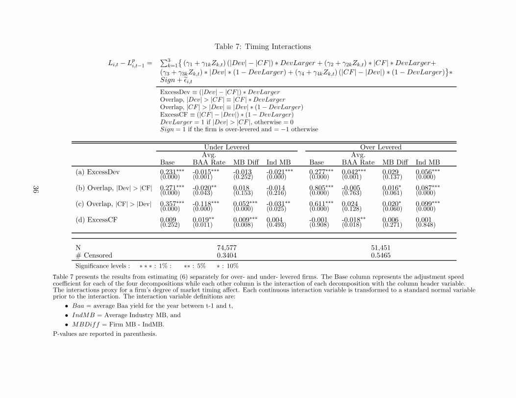
Table 7: Timing Interactions

Li,t − Lpi,t−1

=∑

3

k=1

{(γ1 + γ1kZk,t) (|Dev| − |CF |) ∗ DevLarger + (γ2 + γ2kZk,t) ∗ |CF | ∗ DevLarger+

(γ3 + γ3kZk,t) ∗ |Dev| ∗ (1 − DevLarger) + (γ4 + γ4kZk,t) (|CF | − |Dev|) ∗ (1 − DevLarger)}∗

Sign + εi,t

ExcessDev ≡ (|Dev| − |CF |) ∗ DevLarger

Overlap, |Dev| > |CF | ≡ |CF | ∗ DevLarger

Overlap, |CF | > |Dev| ≡ |Dev| ∗ (1 − DevLarger)ExcessCF ≡ (|CF | − |Dev|) ∗ (1 − DevLarger)DevLarger = 1 if |Dev| > |CF |, otherwise = 0Sign = 1 if the firm is over-levered and = −1 otherwise

Under Levered Over LeveredAvg. Avg.

Base BAA Rate MB Diff Ind MB Base BAA Rate MB Diff Ind MB

(a) ExcessDev 0.231∗∗∗ -0.015∗∗∗ -0.013 -0.021∗∗∗ 0.277∗∗∗ 0.042∗∗∗ 0.029 0.056∗∗∗(0.000) (0.001) (0.252) (0.000) (0.000) (0.001) (0.137) (0.000)

(b) Overlap, |Dev| > |CF| 0.271∗∗∗ -0.020∗∗ 0.018 -0.014 0.805∗∗∗ -0.005 0.016∗ 0.087∗∗∗(0.000) (0.043) (0.153) (0.216) (0.000) (0.763) (0.061) (0.000)

(c) Overlap, |CF| > |Dev| 0.357∗∗∗ -0.118∗∗∗ 0.052∗∗∗ -0.031∗∗ 0.611∗∗∗ 0.024 0.020∗ 0.099∗∗∗(0.000) (0.000) (0.000) (0.025) (0.000) (0.128) (0.060) (0.000)

(d) ExcessCF 0.009 0.019∗∗ 0.009∗∗∗ 0.004 -0.001 -0.018∗∗ 0.006 0.001(0.252) (0.011) (0.008) (0.493) (0.908) (0.018) (0.271) (0.848)

N 74,577 51,451# Censored 0.3404 0.5465

Significance levels : ∗ ∗ ∗ : 1% : ∗∗ : 5% ∗ : 10%

Table 7 presents the results from estimating (6) separately for over- and under- levered firms. The Base column represents the adjustment speedcoefficient for each of the four decompositions while each other column is the interaction of each decomposition with the column header variable.The interactions proxy for a firm’s degree of market timing affect. Each continuous interaction variable is transformed to a standard normal variableprior to the interaction. The interaction variable definitions are:

• Baa = average Baa yield for the year between t-1 and t,

• IndMB = Average Industry MB, and

• MBDiff = Firm MB - IndMB.

P-values are reported in parenthesis.

36