1

Volumetric Analysis & Three-Dimensional Visualization of Industrial Mineral Deposits

By James P. Reed RockWare Incorporated, 2221 East Street, Suite 101, Golden, Colorado 80401

Email: jim@rockware.com Phone: 303-278-3534 Extension 113

Table of Contents Table of Figures.............................................................................................................................................................1 ABSTRACT ..................................................................................................................................................................2 INTRODUCTION.........................................................................................................................................................2

Geological Complexities........................................................................................................................... 3 Economic Complexities ............................................................................................................................ 3

DATA MANAGEMENT ..............................................................................................................................................3 Non-Borehole Data ................................................................................................................................... 5 Borehole Data ........................................................................................................................................... 5

MODELING..................................................................................................................................................................6 Two-Dimensional Modeling (Gridding)................................................................................................... 8 Three-Dimensional Block Modeling ...................................................................................................... 10 Modeling Strategies ................................................................................................................................ 10 Multivariate Modeling ............................................................................................................................ 12

Sand & Gravel Case Study.................................................................................................................. 14 VISUALIZATIONS (DIAGRAMS) ...........................................................................................................................16 VOLUMETRIC COMPUTATIONS...........................................................................................................................20 GLOSSARY................................................................................................................................................................22 REFERENCES ............................................................................................................................................................24

Table of Figures Figure 1: Glacial outwash. (Source: U.S. Geological Survey) ........................................................................................................ 3 Figure 2: Process flowchart depicting transformation of data into reports....................................................................................... 4 Figure 3: Primary Types of Geological Models............................................................................................................................... 7 Figure 4: "Hybrid" model ................................................................................................................................................................ 8 Figure 5: Map depicting clay thicknesses encountered within nine boreholes................................................................................. 8 Figure 6: Map depicting imaginary grid superimposed over project area. ....................................................................................... 8 Figure 7: Color-coded clay thickness estimations............................................................................................................................ 9 Figure 8: Converting a numerical grid model into a color-coded contour map................................................................................ 9 Figure 9: Block Modeling.............................................................................................................................................................. 10 Figure 10: Modeling strategies with examples .............................................................................................................................. 11 Figure 11: Agricultural limestone characteristic maps overlaid to determine optimum area for mining. ...................................... 12 Figure 12: Agricultural limestone characteristic models multiplied together to determine optimum area for mining. .................. 13 Figure 13: Percent Sand/Gravel/Clay three-dimensional log diagrams.......................................................................................... 15 Figure 14: Percent Sand/Gravel/Clay three-dimensional block models ......................................................................................... 15 Figure 15: Percent Sand/Gravel/Clay filtered block models .......................................................................................................... 15 Figure 16: Filtered & combined models ........................................................................................................................................ 16 Figure 17: Preliminary pit designs ................................................................................................................................................. 16 Figure 18: Methods for Visualizing Grid & Block Diagrams ........................................................................................................ 17 Figure 19: Methods for Visualizing Grid & Block Diagrams (cont.)............................................................................................. 18 Figure 20: Grid model representing estimated clay thickness values............................................................................................ 20 Figure 21: Grid model representing estimated clay thickness values greater than five meters. .................................................... 20 Figure 22: Pit Optimization ........................................................................................................................................................... 21 Figure 23: Optimized sand & gravel resource ............................................................................................................................... 21

2

ABSTRACT Base and precious metal deposits are typically characterized by a single parameter such as the total weight of mineable gold. Industrial mineral deposits, on the other hand, are characterized by their end-use. For example, the volumetric evaluation of a limestone deposit depends upon who’s buying the product. The concrete industry has a suite of evaluation parameters such as silica content and abrasion coefficients. Conversely, pharmaceutical-grade limestone buyers are more focused on the calcium/magnesium ratio and various impurities. As a consequence, many industrial mineral deposits must be re-evaluated as the nature of the demand changes. Different customers mean different specifications. Quarry configurations are therefore indirectly determined by the end-product requirements set forth by the customer. This is the ugly reality of industrial mineral mining that is unappreciated by our base/precious-metal colleagues.

Computerized deposit modeling provides a means for tailoring a mine plan based on the end-use specifications. The basic strategy involves the creation of a borehole database that includes analytical results for various physical and chemical properties as a function of depth. Once the database has been created, visualizations such as cross-sections, fence diagrams, and block diagrams may be quickly generated to check the validity and geological reasonability of the modeling. The next step involves the calculation of volumetrics and optimal pit-designs based on a series of user-defined parameters.

The foundation of these analyses involve the creation of imaginary block models in which a site is subdivided into a series of three-dimensional cells called "voxels" (a medical term for volumetric elements). Values are estimated for these voxels based on their proximity relative to downhole data. For example, a clay deposit may involve the creation of separate models representing shrinkage, brightness, and slip. These models are then filtered and combined into a final model that shows where all of the parameters (models) meet a set of user-defined criteria. The net result is high-grade, or "surgical" mining in which the quarry is designed to maximize profitability rather than simply mining the entire lease and relying on the sorting/milling process to separate the ore and the non-ore.

A healthy level of skepticism must be employed when using computer software to compute resource volumetrics. The algorithms or methods used to create the volumetric models have limitations that may be acceptable for one type of deposit while being completely inappropriate for another. For example, a sand and gravel deposit requires an approach that is completely different than the methods used to evaluate a phosphate reserve. The best way to avoid misuse is to always compare "slices" through the models with borehole logs that show the original data. These cross-sections are used to make sure that the model "honors" the data. Just as importantly, cross-sections should be evaluated to make sure that the modeling conforms to the expected geology.

The era of guesstimates has been terminated by the Sarbanes-Oxley Act of 2002. Computerized modeling of industrial mineral reserves provides an inexpensive tool for accurately and quickly estimating volumetrics within a changing marketplace.

INTRODUCTION Computerized evaluations of industrial mineral deposits have been in use since the late 1950s. Since that time, the public-domain and commercial software has become more sophisticated and easier (in a relative sense) to use. This paper describes the methods that are used by these programs. It is important to note that these descriptions are not intended to be performed manually. Instead, the intent is to demystify the "black box" and create an understanding of the advantages and limitations of automated resource computations.

The modeling and economic evaluation of industrial mineral deposits can range from simple to complex. A simple example might involve the evaluation of a clay deposit for geo-membranes at a landfill. Conversely, a complex example would involve the evaluation of the same deposit for use as a rubber additive. These complexities exist on two levels; geological and economic.

3

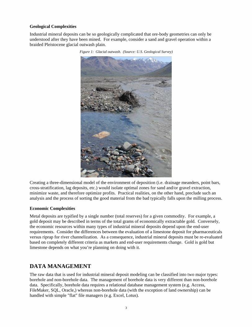
Geological Complexities

Industrial mineral deposits can be so geologically complicated that ore-body geometries can only be understood after they have been mined. For example, consider a sand and gravel operation within a braided Pleistocene glacial outwash plain.

Figure 1: Glacial outwash. (Source: U.S. Geological Survey)

Creating a three-dimensional model of the environment of deposition (i.e. drainage meanders, point bars, cross-stratification, lag deposits, etc.) would isolate optimal zones for sand and/or gravel extraction, minimize waste, and therefore optimize profits. Practical realities, on the other hand, preclude such an analysis and the process of sorting the good material from the bad typically falls upon the milling process.

Economic Complexities

Metal deposits are typified by a single number (total reserves) for a given commodity. For example, a gold deposit may be described in terms of the total grams of economically extractable gold. Conversely, the economic resources within many types of industrial mineral deposits depend upon the end-user requirements. Consider the differences between the evaluation of a limestone deposit for pharmaceuticals versus riprap for river channelization. As a consequence, industrial mineral deposits must be re-evaluated based on completely different criteria as markets and end-user requirements change. Gold is gold but limestone depends on what you’re planning on doing with it.

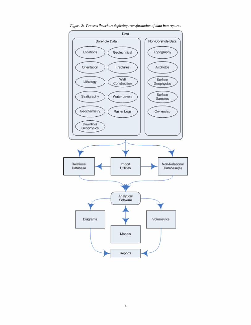
DATA MANAGEMENT The raw data that is used for industrial mineral deposit modeling can be classified into two major types: borehole and non-borehole data. The management of borehole data is very different than non-borehole data. Specifically, borehole data requires a relational database management system (e.g. Access, FileMaker, SQL, Oracle,) whereas non-borehole data (with the exception of land ownership) can be handled with simple "flat" file managers (e.g. Excel, Lotus).

4

Figure 2: Process flowchart depicting transformation of data into reports.

5

Non-Borehole Data

Non-borehole data includes airphotos, land ownership, surface geochemistry, surface geophysics, and topography. These datasets are typically stored in separate files. Organizing these disparate data sets into a single database with downhole data is a somewhat Sisyphean task. Instead, most software will read these files in their native format.

Non-Borehole Data Types

Data Type File Format

Airphotos: GeoTIFF (Tagged Image File Format) with embedded geographic information. JPEG (Joint Photographic Experts Group) PNG (Portable Network Graphics) TIFF (Tagged Image File Format)

Land Ownership: DBF (IBM DataBase File) and SHP (ESRI Shape File)

Topography: DEM (Digital Elevation Model) DXF (AutoCAD data eXchange Format)

Surface Geochemistry:

ASCII (American Standard Code for Information Interchange) XLS (Microsoft Excel)

Surface Geophysics:

Many vendor-specific formats.

Borehole Data

Borehole data may include lithology, stratigraphy, geochemistry, downhole geophysics, geotechnical properties, and water levels. Borehole data cannot be stored in simple "flat" files (e.g. Excel spreadsheets) due to the relational nature of the data. Instead, downhole data must be stored within a relational database in which data-specific tables are linked to a master list of boreholes. The reason for this structure is based on the fact that downhole data is highly variable. For example, one borehole may contain compaction analyses that are sampled on 5-meter intervals while another borehole is sampled at 1-meter intervals. Storing this type of information in a spreadsheet is impractical

Borehole Data Types

Data Type Description / Examples

Location Information

Borehole ID, X and Y location coordinates (Eastings and Northings), surface elevation, total depth, map symbol, comments, range, township, section, legal description, longitude, latitude, etc

Orientation Downhole survey information (depths, bearings, and inclination).

Lithology Observed downhole lithologies (as opposed to interpreted

6

stratigraphy).

Stratigraphy Interpreted downhole stratigraphic data.

Quantitative Interval-Based Data

Downhole data that was sampled over one or more depth intervals, such as geochemical or geotechnical measurements.

Quantitative Point-Based Data

Downhole data that was sampled at individual points, such as geophysical or geotechnical measurements

Fractures Sub-surface fractures information (dip direction, dip amount, aperature, etc.)

Water Levels

Dates and water levels for the borehole.

Raster Images

Raster images (e.g. core, photomicrographs, cuttings, etc.)

Borehole Construction

Construction materials at particular depths and diameters.

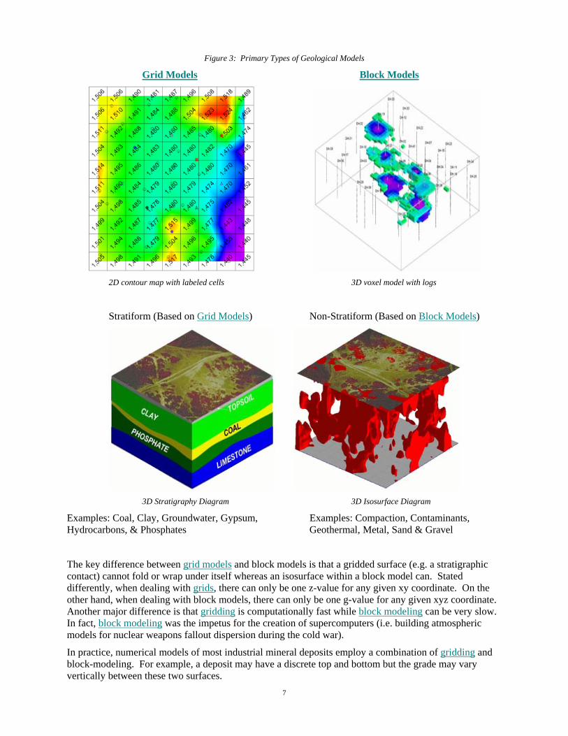
MODELING "Modeling" refers to the process of creating a spatial array of estimations. The parameter that is being estimated may be the thickness of the ore, the grade of the ore, or some other property that is useful for the evaluation of the resource. These arrays may be two or three-dimensional depending upon the number of independent variables. In a two-dimensional array (also referred to as a "grid model"), the dependent variable (z) is a function of the horizontal (x,y) coordinates. In a three-dimensional array (also referred to as a solid or block model), the dependent variable (g) is a function of the horizontal (x,y) and vertical coordinates (z). Grids are used to model topography, stratigraphic contacts, isopachs, and water levels, while solids are used to model geochemistry, ore grades, and geotechnical properties.

7

Figure 3: Primary Types of Geological Models

Grid Models Block Models

2D contour map with labeled cells 3D voxel model with logs

Stratiform (Based on Grid Models) Non-Stratiform (Based on Block Models)

3D Stratigraphy Diagram 3D Isosurface Diagram

Examples: Coal, Clay, Groundwater, Gypsum, Examples: Compaction, Contaminants, Hydrocarbons, & Phosphates Geothermal, Metal, Sand & Gravel

The key difference between grid models and block models is that a gridded surface (e.g. a stratigraphic contact) cannot fold or wrap under itself whereas an isosurface within a block model can. Stated differently, when dealing with grids, there can only be one z-value for any given xy coordinate. On the other hand, when dealing with block models, there can only be one g-value for any given xyz coordinate. Another major difference is that gridding is computationally fast while block modeling can be very slow. In fact, block modeling was the impetus for the creation of supercomputers (i.e. building atmospheric models for nuclear weapons fallout dispersion during the cold war).

In practice, numerical models of most industrial mineral deposits employ a combination of gridding and block-modeling. For example, a deposit may have a discrete top and bottom but the grade may vary vertically between these two surfaces.

8

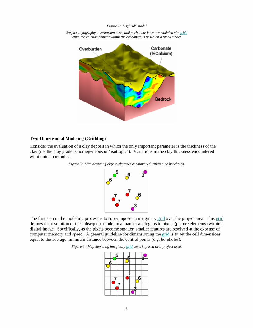
Figure 4: "Hybrid" model

Surface topography, overburden base, and carbonate base are modeled via grids while the calcium content within the carbonate is based on a block model.

Two-Dimensional Modeling (Gridding)

Consider the evaluation of a clay deposit in which the only important parameter is the thickness of the clay (i.e. the clay grade is homogeneous or "isotropic"). Variations in the clay thickness encountered within nine boreholes.

Figure 5: Map depicting clay thicknesses encountered within nine boreholes.

The first step in the modeling process is to superimpose an imaginary grid over the project area. This grid defines the resolution of the subsequent model in a manner analogous to pixels (picture elements) within a digital image. Specifically, as the pixels become smaller, smaller features are resolved at the expense of computer memory and speed. A general guideline for dimensioning the grid is to set the cell dimensions equal to the average minimum distance between the control points (e.g. boreholes).

Figure 6: Map depicting imaginary grid superimposed over project area.

9

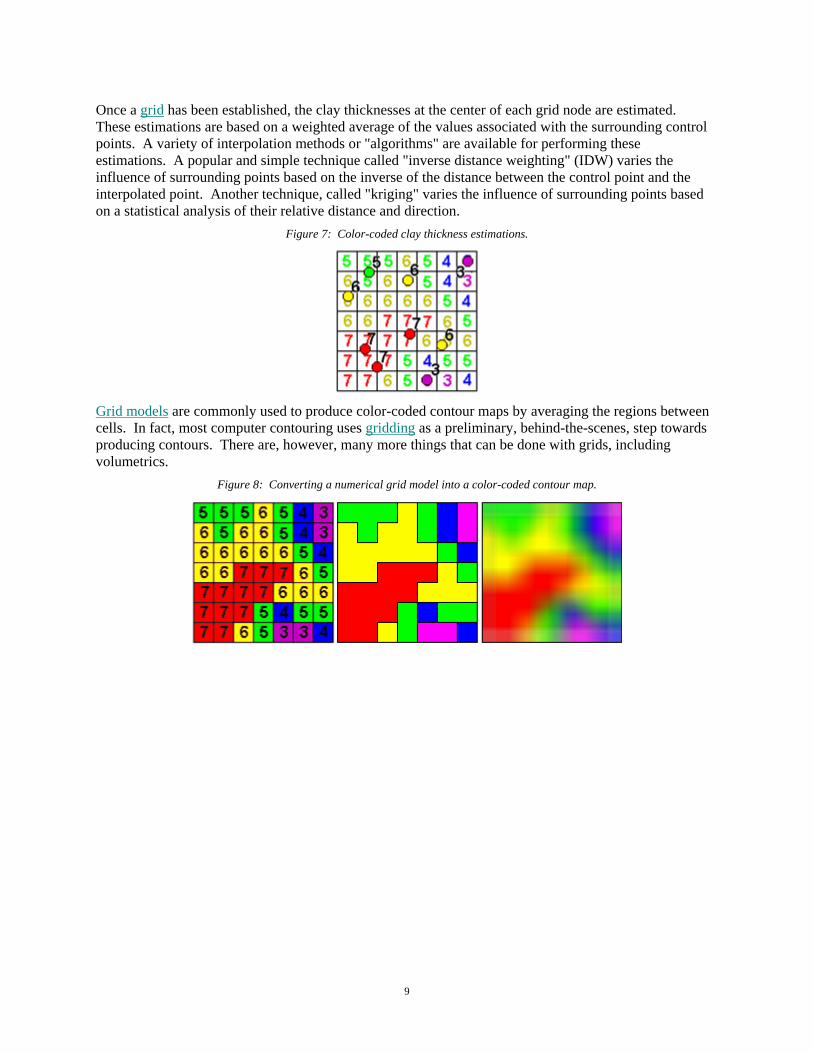
Once a grid has been established, the clay thicknesses at the center of each grid node are estimated. These estimations are based on a weighted average of the values associated with the surrounding control points. A variety of interpolation methods or "algorithms" are available for performing these estimations. A popular and simple technique called "inverse distance weighting" (IDW) varies the influence of surrounding points based on the inverse of the distance between the control point and the interpolated point. Another technique, called "kriging" varies the influence of surrounding points based on a statistical analysis of their relative distance and direction.

Figure 7: Color-coded clay thickness estimations.

Grid models are commonly used to produce color-coded contour maps by averaging the regions between cells. In fact, most computer contouring uses gridding as a preliminary, behind-the-scenes, step towards producing contours. There are, however, many more things that can be done with grids, including volumetrics.

Figure 8: Converting a numerical grid model into a color-coded contour map.

10

Three-Dimensional Block Modeling

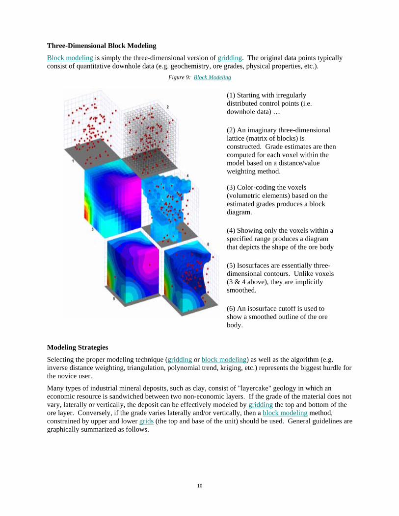
Block modeling is simply the three-dimensional version of gridding. The original data points typically consist of quantitative downhole data (e.g. geochemistry, ore grades, physical properties, etc.).

Figure 9: Block Modeling

(1) Starting with irregularly distributed control points (i.e. downhole data) …

(2) An imaginary three-dimensional lattice (matrix of blocks) is constructed. Grade estimates are then computed for each voxel within the model based on a distance/value weighting method.

(3) Color-coding the voxels (volumetric elements) based on the estimated grades produces a block diagram.

(4) Showing only the voxels within a specified range produces a diagram that depicts the shape of the ore body

(5) Isosurfaces are essentially three-dimensional contours. Unlike voxels (3 & 4 above), they are implicitly smoothed.

(6) An isosurface cutoff is used to show a smoothed outline of the ore body.

Modeling Strategies

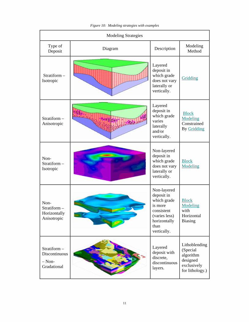
Selecting the proper modeling technique (gridding or block modeling) as well as the algorithm (e.g. inverse distance weighting, triangulation, polynomial trend, kriging, etc.) represents the biggest hurdle for the novice user.

Many types of industrial mineral deposits, such as clay, consist of "layercake" geology in which an economic resource is sandwiched between two non-economic layers. If the grade of the material does not vary, laterally or vertically, the deposit can be effectively modeled by gridding the top and bottom of the ore layer. Conversely, if the grade varies laterally and/or vertically, then a block modeling method, constrained by upper and lower grids (the top and base of the unit) should be used. General guidelines are graphically summarized as follows.

11

Figure 10: Modeling strategies with examples

Modeling Strategies

Type of Deposit Diagram Description Modeling

Method

Stratiform – Isotropic

Layered deposit in which grade does not vary laterally or vertically.

Gridding

Stratiform – Anisotropic

Layered deposit in which grade varies laterally and/or vertically.

Block Modeling Constrained By Gridding

Non-Stratiform – Isotropic

Non-layered deposit in which grade does not vary laterally or vertically.

Block Modeling

Non-Stratiform – Horizontally Anisotropic

Non-layered deposit in which grade is more consistent (varies less) horizontally than vertically.

Block Modeling with Horizontal Biasing

Stratiform – Discontinuous

– Non-Gradational

Layered deposit with discrete, discontinuous layers.

Lithoblending (Special algorithm designed exclusively for lithology.)

12

Multivariate Modeling

The economics of industrial mineral deposits are often determined by more than one property. These properties are often dictated by the end-user specifications. Additionally, a given deposit may be quarried for more than one end-user, each with their own set of material requirements. It is therefore necessary that deposits be modeled for multiple attributes.

Sample Variables Associated With Different Types of Industrial Minerals

Commodity Pertinent Parameters (Specifications)

Aggregates Aggregate Abrasion Value (AAV), Aggregate Crushing Value (ACV), Ten Percent Fines Value (TFV), Aggregate Impact Value (AIV), Polished Stone Value (PSV) Artificial Aggregates (Hardness), Magnesium Sulphate Soundness Value (MSSV), Aggregate Size, Aggregate Grading, Flakiness, Grading Zone, Moisture Content, Water Absorption, & Frost Susceptibility

Agricultural Limestone

Dry Weight Analysis, Percent Calcium, Percent Magnesium, Percent Magnesium Oxide, Percent Calcium Oxide, Calcium Carbonate Equivalent (CCE), Effective Neutralizing Value (ENV), Screen Test Results,

Filler-Grade Clay

Cone, Fired Color, Fired Shrinkage, Water Absorption, Reflectance, Brightness, Specific Gravity, Mohs Hardness, Moisture Content, Chemical Content, Particle Size Distribution

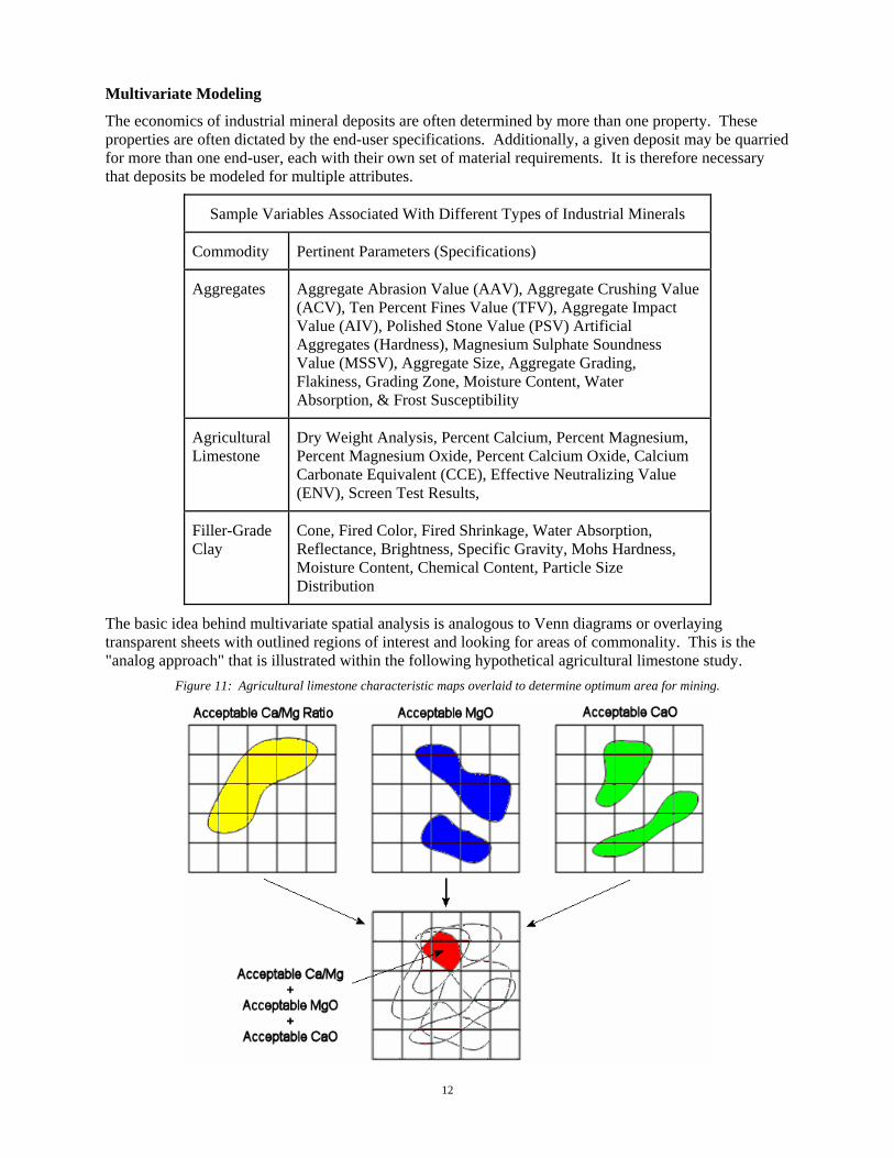
The basic idea behind multivariate spatial analysis is analogous to Venn diagrams or overlaying transparent sheets with outlined regions of interest and looking for areas of commonality. This is the "analog approach" that is illustrated within the following hypothetical agricultural limestone study.

Figure 11: Agricultural limestone characteristic maps overlaid to determine optimum area for mining.

13

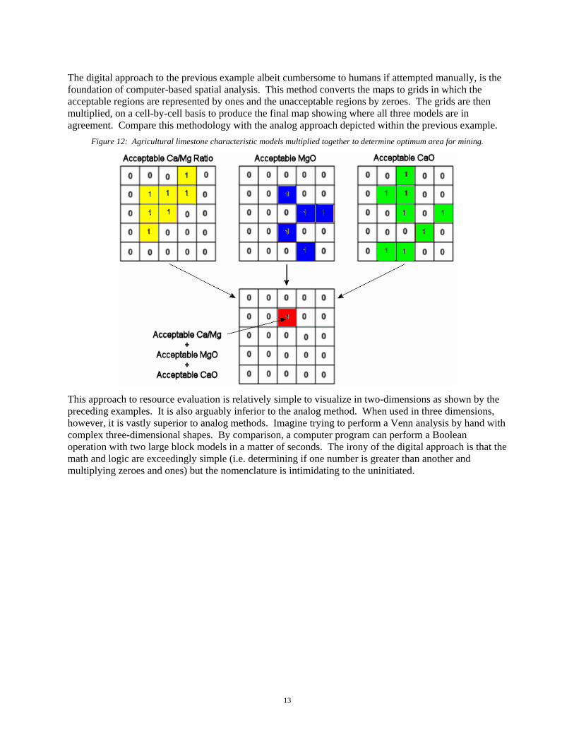
The digital approach to the previous example albeit cumbersome to humans if attempted manually, is the foundation of computer-based spatial analysis. This method converts the maps to grids in which the acceptable regions are represented by ones and the unacceptable regions by zeroes. The grids are then multiplied, on a cell-by-cell basis to produce the final map showing where all three models are in agreement. Compare this methodology with the analog approach depicted within the previous example.

Figure 12: Agricultural limestone characteristic models multiplied together to determine optimum area for mining.

This approach to resource evaluation is relatively simple to visualize in two-dimensions as shown by the preceding examples. It is also arguably inferior to the analog method. When used in three dimensions, however, it is vastly superior to analog methods. Imagine trying to perform a Venn analysis by hand with complex three-dimensional shapes. By comparison, a computer program can perform a Boolean operation with two large block models in a matter of seconds. The irony of the digital approach is that the math and logic are exceedingly simple (i.e. determining if one number is greater than another and multiplying zeroes and ones) but the nomenclature is intimidating to the uninitiated.

14

Sand & Gravel Case Study

In the following case study involving multivariate modeling, a series of exploration boreholes were drilled. Samples were taken every five feet and sieved in order to determine the relative percentages of sand, gravel and clay (or other non-sand/gravel material). These samples were restricted to the interval below the base of the soil profile and the top of the bedrock.

Step 1. The borehole locations, stratigraphy, and sieve analyses were entered into a relational database.

Information Recorded for Each Borehole

Name: Unique borehole identifier (e.g. BH-01, BH-02, etc.)

Easting: UTM easting from GPS (in feet)

Northing: UTM northing from GPS (in feet)

Elevation: Elevation from GPS (in feet)

Soil Depth: Depth to base of soil (in feet).

Bedrock Depth: Depth to top of bedrock (in feet).

Total Depth: Total depth of borehole (in feet).

Information Recorded for Each Sample Interval

Depth-1: Depth to top of sampled interval (feet).

Depth-2: Depth to base of sampled interval (feet).

Sand: % Sand (0 to 100)

Gravel: % Gravel (0 to 100)

Clay: % Clay or other non-sand/gravel material(0 - 100)

Data entry is the most laborious and error-prone step within the entire process or automating resource evaluations. For this reason, it is imperative that diagrams of the "raw" data (see Step 2) be created before attempting the modeling in order to check for errors in the data such as mistyped borehole coordinates, spurious data values, and transposed coordinates. It is also useful to perform simple statistical analyses, such as data histograms to check for unreasonable outliers.

Step 2. Separate three-dimensional percentage log diagrams were created to show the relative concentrations of each constituent (% sand, % gravel, and % clay). The percentages are depicted as color-coded cylinders in which the cylinder radius is proportional to the component concentration while the colors are scaled in a similar fashion from the "cold" colors (purple) through the "hot" colors (red).

15

Figure 13: Percent Sand/Gravel/Clay three-dimensional log diagrams

% Sand % Gravel %Clay

Step 3. Solid "block" models for the sand, gravel, and clay data were created by using a block modeling algorithm and truncated by grid models representing the base of the soil overburden and bedrock (material below the sand/gravel unit). Each of these models was then filtered based on acceptability cutoff levels.

Figure 14: Percent Sand/Gravel/Clay three-dimensional block models

% Sand % Gravel %Clay

Block Models

Step 4. Each of these models was then filtered based on acceptability cutoff levels. Figure 15: Percent Sand/Gravel/Clay filtered block models

% Sand > 40% % Gravel > 40% %Clay < 20%

16

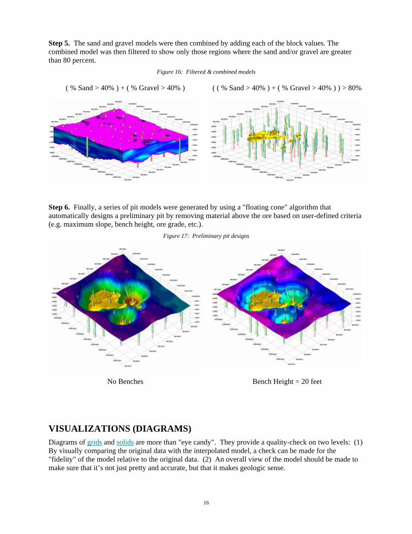
Step 5. The sand and gravel models were then combined by adding each of the block values. The combined model was then filtered to show only those regions where the sand and/or gravel are greater than 80 percent.

Figure 16: Filtered & combined models

( % Sand > 40% ) + ( % Gravel > 40% ) ( ( % Sand > 40% ) + ( % Gravel > 40% ) ) > 80%

Step 6. Finally, a series of pit models were generated by using a "floating cone" algorithm that automatically designs a preliminary pit by removing material above the ore based on user-defined criteria (e.g. maximum slope, bench height, ore grade, etc.).

Figure 17: Preliminary pit designs

No Benches Bench Height = 20 feet

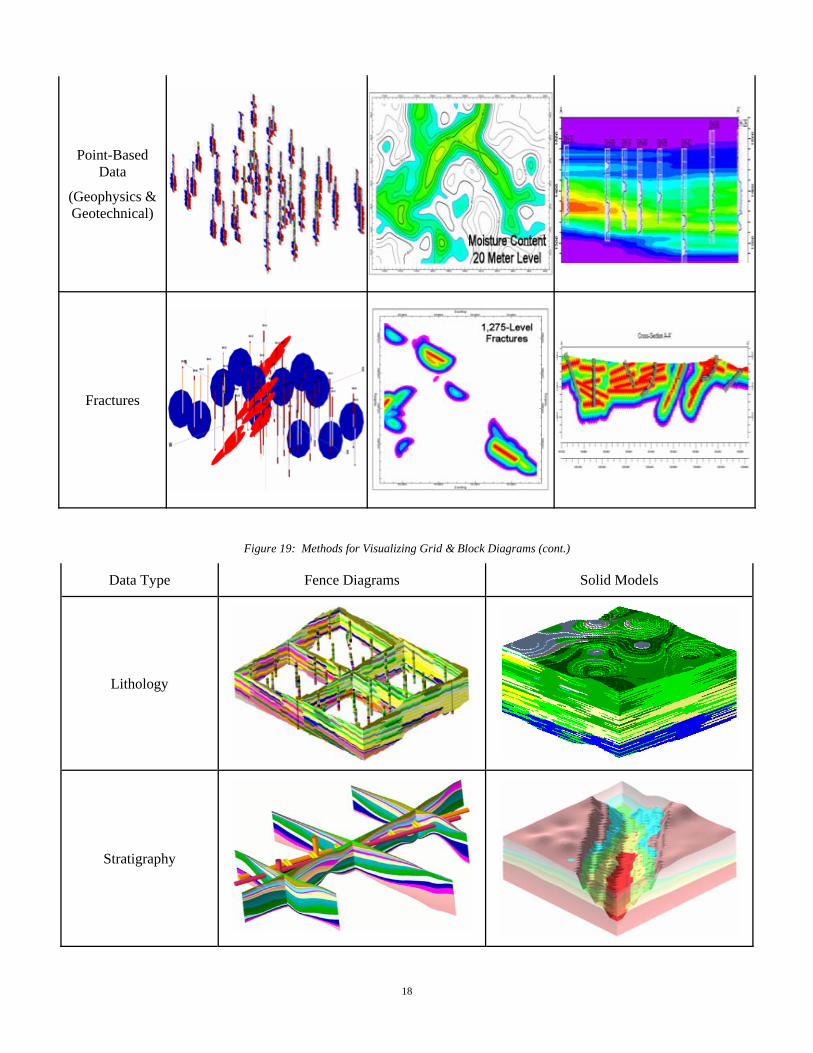
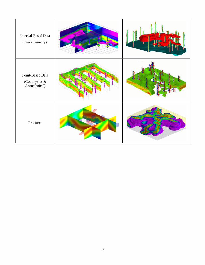
VISUALIZATIONS (DIAGRAMS) Diagrams of grids and solids are more than "eye candy". They provide a quality-check on two levels: (1) By visually comparing the original data with the interpolated model, a check can be made for the "fidelity" of the model relative to the original data. (2) An overall view of the model should be made to make sure that it’s not just pretty and accurate, but that it makes geologic sense.

17

Figure 18: Methods for Visualizing Grid & Block Diagrams

Data Type Striplogs Plan-Views Cross-Sections

Lithology

Stratigraphy

Interval-Based Data

(Geochemistry)

18

Point-Based Data

(Geophysics & Geotechnical)

Fractures

Figure 19: Methods for Visualizing Grid & Block Diagrams (cont.)

Data Type Fence Diagrams Solid Models

Lithology

Stratigraphy

19

Interval-Based Data

(Geochemistry)

Point-Based Data

(Geophysics & Geotechnical)

Fractures

20

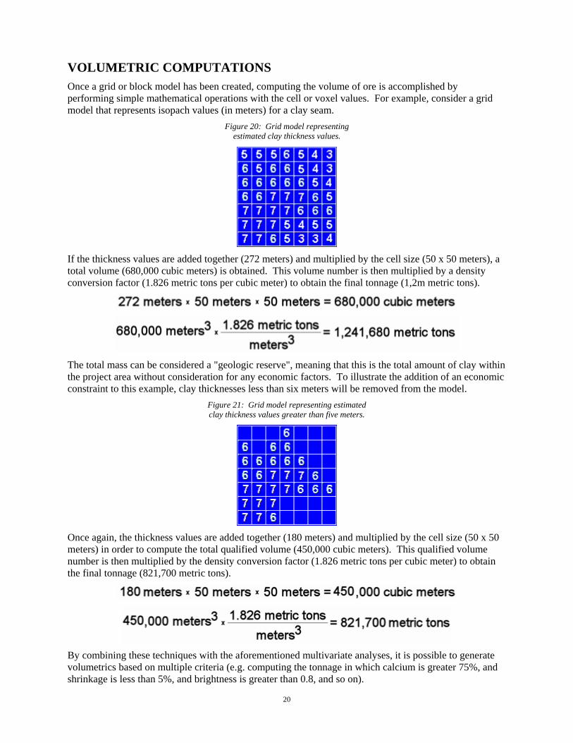
VOLUMETRIC COMPUTATIONS Once a grid or block model has been created, computing the volume of ore is accomplished by performing simple mathematical operations with the cell or voxel values. For example, consider a grid model that represents isopach values (in meters) for a clay seam.

Figure 20: Grid model representing estimated clay thickness values.

If the thickness values are added together (272 meters) and multiplied by the cell size (50 x 50 meters), a total volume (680,000 cubic meters) is obtained. This volume number is then multiplied by a density conversion factor (1.826 metric tons per cubic meter) to obtain the final tonnage (1,2m metric tons).

The total mass can be considered a "geologic reserve", meaning that this is the total amount of clay within the project area without consideration for any economic factors. To illustrate the addition of an economic constraint to this example, clay thicknesses less than six meters will be removed from the model.

Figure 21: Grid model representing estimated clay thickness values greater than five meters.

Once again, the thickness values are added together (180 meters) and multiplied by the cell size (50 x 50 meters) in order to compute the total qualified volume (450,000 cubic meters). This qualified volume number is then multiplied by the density conversion factor (1.826 metric tons per cubic meter) to obtain the final tonnage (821,700 metric tons).

By combining these techniques with the aforementioned multivariate analyses, it is possible to generate volumetrics based on multiple criteria (e.g. computing the tonnage in which calcium is greater 75%, and shrinkage is less than 5%, and brightness is greater than 0.8, and so on).

21

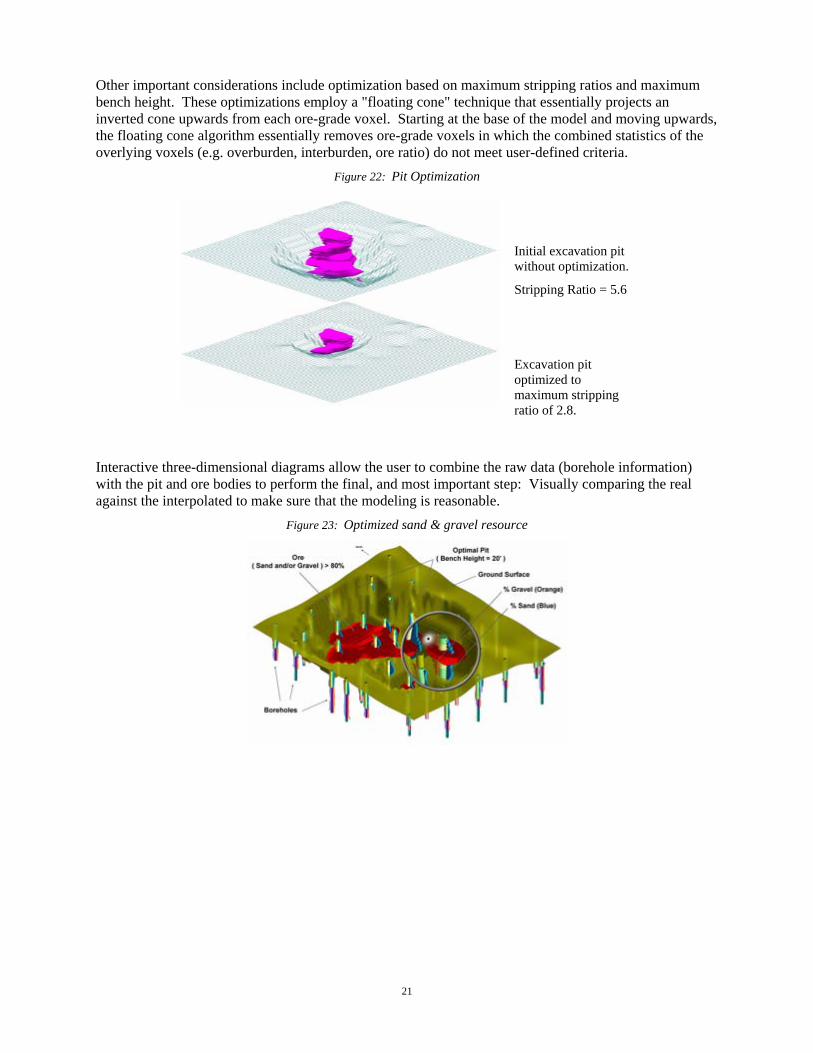
Other important considerations include optimization based on maximum stripping ratios and maximum bench height. These optimizations employ a "floating cone" technique that essentially projects an inverted cone upwards from each ore-grade voxel. Starting at the base of the model and moving upwards, the floating cone algorithm essentially removes ore-grade voxels in which the combined statistics of the overlying voxels (e.g. overburden, interburden, ore ratio) do not meet user-defined criteria.

Figure 22: Pit Optimization

Initial excavation pit without optimization.

Stripping Ratio = 5.6

Excavation pit optimized to maximum stripping ratio of 2.8.

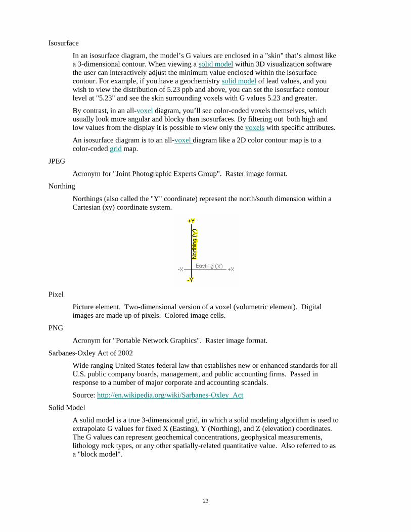
Interactive three-dimensional diagrams allow the user to combine the raw data (borehole information) with the pit and ore bodies to perform the final, and most important step: Visually comparing the real against the interpolated to make sure that the modeling is reasonable.

Figure 23: Optimized sand & gravel resource

22

GLOSSARY ASCII

American Standard Code for Information Interchange file. ASCII files are also referred to as "text" files.

Block Model

See solid model.

Block Modeling

See solid modeling.

Cell

Individual element defined by a grid. The midpoint or attribute of a cell is called the "node". The value associated with a cell is called a "cell value" or "node value".

DEM

Acronym for "Digital Elevation Model". Typically, these files contain gridded data representing topographic elevations.

DBF

Acronym for "IBM DataBase File". Relational database format.

DXF

Acronym for "AutoCAD data eXchange Format". ASCII vector graphics format.

Easting

Eastings (also called the "X" coordinate) represent the east/west dimension within a Cartesian (xy) coordinate system.

GeoTIFF

Acronym for "Tagged Image File Format". Raster image format that includes embedded geographic information.

Grid

Numeric representation of a surface, be it elevations in your study area, formation thickness, or BTU values in a coal seam, to name a few. A grid model or grid file is the computer file of numbers that contains the results of the gridding process. It contains a listing of the X and Y location coordinates of the regularly-spaced grid nodes and the extrapolated Z value at each node. The process of creating a grid is referred to as "gridding".

Gridding

Computer process whereby a grid model is interpolated based on irregularly-spaced control points.

23

Isosurface

In an isosurface diagram, the model’s G values are enclosed in a "skin" that’s almost like a 3-dimensional contour. When viewing a solid model within 3D visualization software the user can interactively adjust the minimum value enclosed within the isosurface contour. For example, if you have a geochemistry solid model of lead values, and you wish to view the distribution of 5.23 ppb and above, you can set the isosurface contour level at "5.23" and see the skin surrounding voxels with G values 5.23 and greater.

By contrast, in an all-voxel diagram, you’ll see color-coded voxels themselves, which usually look more angular and blocky than isosurfaces. By filtering out both high and low values from the display it is possible to view only the voxels with specific attributes.

An isosurface diagram is to an all-voxel diagram like a 2D color contour map is to a color-coded grid map.

JPEG

Acronym for "Joint Photographic Experts Group". Raster image format.

Northing

Northings (also called the "Y" coordinate) represent the north/south dimension within a Cartesian (xy) coordinate system.

Pixel

Picture element. Two-dimensional version of a voxel (volumetric element). Digital images are made up of pixels. Colored image cells.

PNG

Acronym for "Portable Network Graphics". Raster image format.

Sarbanes-Oxley Act of 2002

Wide ranging United States federal law that establishes new or enhanced standards for all U.S. public company boards, management, and public accounting firms. Passed in response to a number of major corporate and accounting scandals.

Source: http://en.wikipedia.org/wiki/Sarbanes-Oxley_Act

Solid Model

A solid model is a true 3-dimensional grid, in which a solid modeling algorithm is used to extrapolate G values for fixed X (Easting), Y (Northing), and Z (elevation) coordinates. The G values can represent geochemical concentrations, geophysical measurements, lithology rock types, or any other spatially-related quantitative value. Also referred to as a "block model".

24

Solid Modeling

Computer process whereby a solid model is interpolated based on irregularly-spaced control points. Also referred to as "block modeling".

SHP

Acronym for "ESRI Shape File". Relational database format.

TIFF

Acronym for "Tagged Image File Format". Raster image format.

Voxel

Volumetric element. The three dimensional version of a pixel (picture element). Solid models are made up of voxels. Grid models are made up of cells.

X

See easting.

Y

See northing.

XLS

Acronym for "Microsoft Excel" spreadsheet files.

REFERENCES Martin Limestone, Undated, Frequently asked questions: http://www.martinlimestone.com/mli/faq/, accessed on April 1st, 2007

RockWare, 2007, RockWorks/2006: Integrated geological data management, analysis, and visualization: http://www.rockware.com, accessed on March 12, 2007.

Summers, C.J., 2006, The idiot’s guide to highways maintenance: http://www.highwaysmaintenance.com/Aggtext.htm, accessed on April 1st, 2007

University of Exeter, 2007, Glossary: http://www.projects.ex.ac.uk/geomincentre/estuary/Main/glossary.htm, accessed on March 20th, 2007.

U.S. Geological Survey, 2007, Photos taken during field work for the Yukon Project, http://infotrek.er.usgs.gov/mercury/yukon_photos.html, accessed on April 1st, 2007.