case study analysis of bimodal branched polyethylene...

www.jordilabs.com

CASE STUDY Analysis of Bimodal Branched Polyethylene on Resolve GPC

STUDY The goal of this analysis was to analyze a series of bimodal polyethylene samples to determine the extent of long chain branching and the absolute and relative molecular weights. ANALYTICAL STRATEGY The samples were analyzed using Resolve GPC columns with both conventional calibration (relative to polystyrene standards) and absolute molecular weight determination with light scattering, viscometry and refractive index detection (GPC-HT). CONCLUSIONS The samples were found to have significantly different extents of long chain branching in spite of the fact that their molecular weight distributions looked very similar by conventional GPC-H analysis. The absolute molecular weight of the samples was also observed to vary significantly from the relative molecular weight. Even more importantly, the largest sample as determined by conventional GPC-H was Sample 2 while in GPC-HT the largest sample was Sample 1. This was shown to correspond to an increase in long chain branching in Sample 1. These results reveal the importance of GPC-HT for characterization of more complex polymer architectures. Read the following report to see the full analysis.

Company Name Contact Name

Released by:

Mark Jordi, Ph.D. President

Job Number: JXXXX

CONFIDENTIAL

Date Client Name Company Name Address Dear Valued Client, Please find enclosed the test results for your samples described as:

1. Sample 1 2. Sample 2 3. Sample 3

The following tests were performed:

1. High Temperature Gel Permeation Chromotagraphy (GPC-H) 2. High Temperature Tetradetection Gel Permeation Chromatography (GPC-HT)

Objective The goal of this analysis was to determine the relative and absolute molecular weight distributions and branching structures of the polyethylene samples using Jordi Resolve 13 µm Mixed Bed GPC columns. Summary of Results Three samples were subjected to GPC-H and GPC-HT analysis. The results for GPC-H and GPC-HT are summarized in Table 1 and Table 3, respectively. Table 4 includes the Mark Houwink data. Analysis results by GPC-H indicated that Sample 2 had the largest molecular weight (~502K) followed by sample 3 (458K) and sample 1 (394K). In contrast, GPC-T analysis results determined that that sample 1 was in fact the largest sample (253K), followed by sample 3 (186K) and then sample 2 (174K). A downward curvature of the Mark Houwink plots at high molecular weight indicated that the samples are branched polymers (long chain branching). The branch frequency in the samples was calculated using a NIST linear standard and are shown in Table 4. Samples 1, 2 and 3 showed branching frequencies per 1000 carbons of 4.8, 1.5 and 3.7 respectively.

It is expected that the GPC-HT results are a more accurate reflection of the true sample molecular weight than the GPC-H results, because the polystyrene calibrant is structurally different from the sample polyethylene being characterized. This has a significant effect on the calculated molecular weight averages. It is further noted that the presence of branching in the samples results in similar distribution shapes for the three samples even though the molecular weights are in fact significantly different. The increased branching frequency in sample 1 corresponds with the higher molecular weight for this sample. The use of GPC-HT provides significantly more insight into the true molecular weight distributions and polymer architecture of the samples. Individual Test Results A summary of the individual test results is provided below. All accompanying data, including spectra, has been included in the data section of this report. GPC GPC Background: A polymer is a large molecule which is formed using a repeating subunit. A polymeric sample does not have a single molecular weight but rather a range of values and thus an average value is used to indicate its molecular weight. Three different molecular weight averages are commonly used to provide information about polymers. These are the number average molecular weight (Mn), the weight average molecular weight (Mw), and the Z average molecular weight (Mz). Mn provides information about the lowest molecular weight portion of the sample. Mw is the average closest to the center of the peak and Mz represents the highest molecular weight portion of the sample. The different molecular weight averages can each be related to specific polymer properties such as material toughness, tensile strength, and total elongation. By comparing the different averages, it is possible to define a fourth parameter called the polydispersity index (PDI). This parameter gives an indication of how broad a range of molecular weights are in the sample. Enclosed are refractive index chromatograms for each sample, as well as their cumulative weight fraction curves, molecular weight distribution curves and summary reports. A second summary report for each sample is included to show the reproducibility of the data. A calibration curve and chromatographic overlay of the standards are included. Also, please find an overlay of the sample with standards. Results: Analysis by GPC requires that a suitable solvent be found to dissolve the samples. The samples were found to dissolve in Trichlorobenzene (TCB). Enclosed are refractive index chromatograms for the samples, as well as cumulative weight fraction curves, and molecular weight distribution curves. A calibration curve and chromatographic overlay of the standards are also included. The average molecular weights are summarized in Table 1. The samples were

analyzed relative to polystyrene standards as polyethylene standards are not available. The polystyrene calibrant is structurally different from the sample polyethylene being characterized. This results in an increase in the calculated molecular weight averages when compared to absolute molecular weight values.

Table 1. Average Molecular Weight

Relative to polystyrene standards

NIST Polyethylene 1484a (Mw= 119,600 Da)


Sample 1

Sample 2

Sample 3

Sample Mn Mw Mz Mw/Mn

2016-01-29_19;30;12_PE_linear_NISt_std_1484a_01.vdt 281,229 329,170 385,848 1.170

2016-01-29_20;33;45_PE_linear_NISt_std_1484a_02.vdt 272,778 331,956 398,649 1.217


2016-01-29_21;37;19_PE_linear_NIST_std_1475a__01.vdt 42,325 157,845 503,338 3.729

2016-01-29_22;40;53_PE_linear_NIST_std_1475a__02.vdt 42,082 157,887 498,944 3.752


2016-01-30_07;09;36_IPLEX_01.vdt 18,202 401,051 1.603 e 6 22.033

2016-01-30_08;13;09_IPLEX_02.vdt 18,729 388,312 1.613 e 6 20.732


2016-01-30_09;16;45_CCC#5607_5_01.vdt 19,894 508,972 2.478 e 6 25.583

2016-01-30_10;20;21_CCC#5607_5_02.vdt 19,118 496,870 2.413 e 6 25.989


2016-01-30_11;23;55_HCC_276_18_01.vdt 15,378 464,439 2.326 e 6 30.200

2016-01-30_12;27;31_HCC_276_18_02.vdt 15,397 453,539 2.318 e 6 29.455

Sample_1_01.vdt

Sample 2 01.vdt

Sample_1_02.vdt

Sample 2 02.vdt

Sample 3 01.vdt

Sample 3 02.vdt

Figure 1. Normalized overlay of refractive index (RI) chromatograms of the samples.

Figure 2. Overlay of cumulative weight fraction curves for the samples.

0.0

0.1

0.2

0.3

0.4

0.5

0.6

0.7

0.8

0.9

Cum

ulat

ive

Wei

ght

Fra

ctio

n

100 200 1000 2000 410 42x10 510 52x10 610 62x10 710 72x10 810Molecular Weight (Da)

Red = Sample 1 Purple= Sample 2 Green = Sample 3


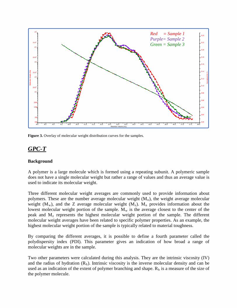
Figure 3. Overlay of molecular weight distribution curves for the samples.

GPC-T Background A polymer is a large molecule which is formed using a repeating subunit. A polymeric sample does not have a single molecular weight but rather a range of values and thus an average value is used to indicate its molecular weight. Three different molecular weight averages are commonly used to provide information about polymers. These are the number average molecular weight (Mn), the weight average molecular weight (Mw), and the Z average molecular weight (Mz). Mn provides information about the lowest molecular weight portion of the sample. Mw is the average closest to the center of the peak and Mz represents the highest molecular weight portion of the sample. The different molecular weight averages have been related to specific polymer properties. As an example, the highest molecular weight portion of the sample is typically related to material toughness. By comparing the different averages, it is possible to define a fourth parameter called the polydispersity index (PDI). This parameter gives an indication of how broad a range of molecular weights are in the sample. Two other parameters were calculated during this analysis. They are the intrinsic viscosity (IV) and the radius of hydration (Rh). Intrinsic viscosity is the inverse molecular density and can be used as an indication of the extent of polymer branching and shape. Rh is a measure of the size of the polymer molecule.

100

200

1000

2000

410

42x10

510

52x10

610

62x10

710

72x10

810M

olec

ular

Wei

ght

(Da)

0.00

0.02

0.04

0.06

0.08

0.10

0.12

0.14

0.16

0.18

0.20

0.22

0.24

Nor

mal

ized

Wt

Fr

8.0 8.5 9.0 9.5 10.0 10.5 11.0 11.5 12.0 12.5 13.0 13.5 14.0 14.5 15.0 15.5 16.0 16.5 17.0 17.5 18.0Retention Volume (mL)


Mark–Houwink Equation The Mark Houwink equation describes the dependence of the intrinsic viscosity of a polymer on its relative molecular mass (molecular weight) and has the form: [IV] = K × Mα Where [IV] is the intrinsic viscosity, K and α are constants, the values of which depend on the nature of the polymer and solvent as well as on temperature and M is the molecular mass. Taking the Log of this equation results in: Log [IV]= Log K + α*Log [M] This equation is linear and has the form: Y = mX+b Where m is the slope and b is the intercept. The Mark Houwink relationship therefore has a slope of α and an intercept of Log K. The slope is an important indicator of how the molecule behaves in solution. A solid sphere will have a Mark Houwink slope of zero, a rigid rod has a slope of two and a random coil should have a slope of 0.7. Thus, the slope is a function of molecular shape. Results Table 2 shows the results of the system suitability standards. One narrow standard (PS 105,453 Da) was used to calibrate the instrument. A broad standard (PS 234,425 Da) along with two NIST PE standards were used as reference standards to verify system performance. Table 3 shows the results for the samples. Figures 1 – 6 show overlays of the Refractive Index (RI), Right Angle Light Scattering (RALS), Viscometer (DP), Molecular Weight Distribution and Mark Houwink curves. Table 4 includes the Mark Houwink data.

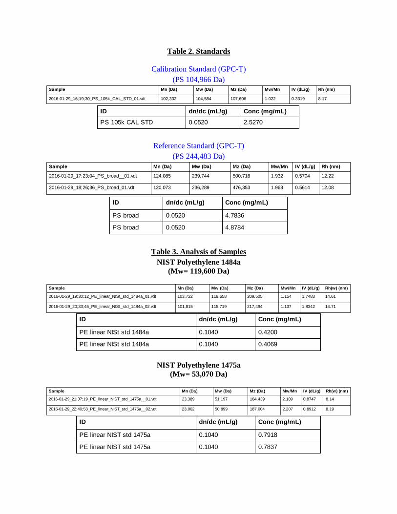
Table 2. Standards

Calibration Standard (GPC-T) (PS 104,966 Da)

Reference Standard (GPC-T) (PS 244,483 Da)

Table 3. Analysis of Samples NIST Polyethylene 1484a

(Mw= 119,600 Da)


Sample Mn (Da) Mw (Da) Mz (Da) Mw/Mn IV (dL/g) Rh (nm)

2016-01-29_16;19;30_PS_105k_CAL_STD_01.vdt 102,332 104,584 107,606 1.022 0.3319 8.17

ID dn/dc (mL/g) Conc (mg/mL)

PS 105k CAL STD 0.0520 2.5270


2016-01-29_17;23;04_PS_broad__01.vdt 124,085 239,744 500,718 1.932 0.5704 12.22

2016-01-29_18;26;36_PS_broad_01.vdt 120,073 236,289 476,353 1.968 0.5614 12.08


PS broad 0.0520 4.7836

PS broad 0.0520 4.8784

Sample Mn (Da) Mw (Da) Mz (Da) Mw/Mn IV (dL/g) Rh(w) (nm)

2016-01-29_19;30;12_PE_linear_NISt_std_1484a_01.vdt 103,722 119,658 209,505 1.154 1.7483 14.61

2016-01-29_20;33;45_PE_linear_NISt_std_1484a_02.vdt 101,815 115,719 217,494 1.137 1.8342 14.71


PE linear NISt std 1484a 0.1040 0.4200

PE linear NISt std 1484a 0.1040 0.4069


2016-01-29_21;37;19_PE_linear_NIST_std_1475a__01.vdt 23,389 51,197 184,439 2.189 0.8747 8.14

2016-01-29_22;40;53_PE_linear_NIST_std_1475a__02.vdt 23,062 50,899 187,004 2.207 0.8912 8.19


PE linear NIST std 1475a 0.1040 0.7918

PE linear NIST std 1475a 0.1040 0.7837

Sample 1

Sample 2

Sample 3


2016-01-30_07;09;36_IPLEX_01.vdt 28,191 259,213 1.348 e 6 9.195 1.6198 14.97

2016-01-30_08;13;09_IPLEX_02.vdt 28,529 247,322 1.393 e 6 8.669 1.5590 14.54


IPLEX 0.1040 1.4280

IPLEX 0.1040 1.4954


2016-01-30_09;16;45_CCC#5607_5_01.vdt 23,071 176,282 583,768 7.641 1.8046 14.35

2016-01-30_10;20;21_CCC#5607_5_02.vdt 23,283 172,045 586,939 7.389 1.7568 14.05


CCC#5607_5 0.1040 1.4053

CCC#5607_5 0.1040 1.4395


2016-01-30_11;23;55_HCC_276_18_01.vdt 20,831 186,723 725,837 8.964 1.6364 13.91

2016-01-30_12;27;31_HCC_276_18_02.vdt 21,515 187,158 748,085 8.699 1.5854 13.67


HCC 276_18 0.1040 1.4769

HCC 276_18 0.1040 1.4949

Sample_1_01.vdt

Sample_1_02.vdt

Sample_1_01.vdt

Sample_1_02.vdt

Sample_2_01.vdt Sample_2_02.vdt




Figure 4. Overlay of normalized refractive index (RI) sample chromatograms.

Figure 5. Overlay of normalized right angle light scattering (RALS) sample chromatograms.



Figure 6. Overlay of normalized Viscometer (DP) sample chromatograms.

Figure 7. Overlay of cumulative weight fraction curves for all samples.

0.0

0.1

0.2

0.3

0.4

0.5

0.6

0.7

0.8

0.9

1.0

Cum

ulat

ive

Wei

ght

Fra

ctio

n

1000 2000 3000 410 42x10 43x10 510 52x10 53x10 610 62x10 63x10 710 72x10 73x10Molecular Weight (Da)



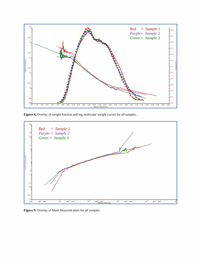
Figure 8. Overlay of weight fraction and log molecular weight curves for all samples.

Figure 9. Overlay of Mark Houwink plots for all samples.

1000

2000

410

42x10

510

52x10

610

62x10

710

72x10

810M

olec

ular

Wei

ght

(Da)

0.00

0.02

0.04

0.06

0.08

0.10

0.12

0.14

0.16

0.18

0.20

0.22

0.24

Nor

mal

ized

Wt

Fr

7.0 7.5 8.0 8.5 9.0 9.5 10.0 10.5 11.0 11.5 12.0 12.5 13.0 13.5 14.0 14.5 15.0 15.5 16.0 16.5 17.0 17.5 18.0 18.5 19.0 19.5 20.0Retention Volume (mL)

-310

-32x10

0.01

0.02

0.1

0.2

1

2

10

20

100

200

1000

Intr

insi

c V

isco

sity

(dL/

g)

1000 2000 3000 410 42x10 43x10 510 52x10 53x10 610 62x10 63x10 710 72x10 73x10 810Molecular Weight (Da)


Red = Sample 1 Purple = Sample 2 Green = Sample 3

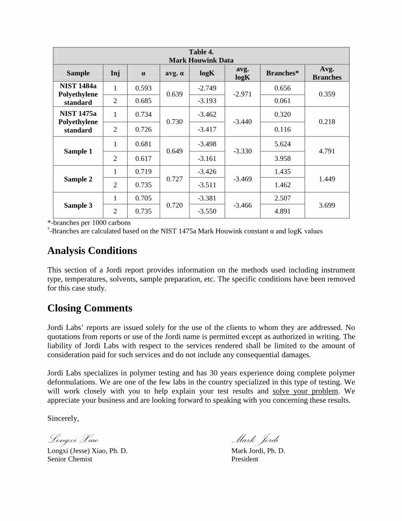
Table 4. Mark Houwink Data

Sample Inj α avg. α logK avg. logK Branches* Avg.

Branches NIST 1484a Polyethylene

standard

1 0.593 0.639

-2.749 -2.971

0.656 0.359

2 0.685 -3.193 0.061

NIST 1475a Polyethylene

standard

1 0.734 0.730

-3.462 -3.440

0.320 0.218

2 0.726 -3.417 0.116

Sample 1 1 0.681

0.649 -3.498

-3.330 5.624

4.791 2 0.617 -3.161 3.958

Sample 2 1 0.719

0.727 -3.426

-3.469 1.435

1.449 2 0.735 -3.511 1.462

Sample 3 1 0.705

0.720 -3.381

-3.466 2.507

3.699 2 0.735 -3.550 4.891

*-branches per 1000 carbons †-Branches are calculated based on the NIST 1475a Mark Houwink constant α and logK values Analysis Conditions This section of a Jordi report provides information on the methods used including instrument type, temperatures, solvents, sample preparation, etc. The specific conditions have been removed for this case study. Closing Comments Jordi Labs’ reports are issued solely for the use of the clients to whom they are addressed. No quotations from reports or use of the Jordi name is permitted except as authorized in writing. The liability of Jordi Labs with respect to the services rendered shall be limited to the amount of consideration paid for such services and do not include any consequential damages. Jordi Labs specializes in polymer testing and has 30 years experience doing complete polymer deformulations. We are one of the few labs in the country specialized in this type of testing. We will work closely with you to help explain your test results and solve your problem. We appreciate your business and are looking forward to speaking with you concerning these results. Sincerely, Longxi Xiao Longxi (Jesse) Xiao, Ph. D. Senior Chemist

Mark Jordi Mark Jordi, Ph. D. President

case study analysis of bimodal branched polyethylene...

Documents