case studies of midwestern thundersnow events

CASE STUDIES OF MIDWESTERN THUNDERSNOW EVENTS

————————————————–

A Thesis Presented to the Faculty of the Graduate SchoolUniversity of Missouri-Columbia

————————————————–

In Partial Fulfillment for the DegreeMaster of Science

————————————————–

by

CHRISTOPHER E. HALCOMB

Dr. Patrick S. Market, Thesis Supervisor

DECEMBER 2001

COMMITTEE IN CHARGE OF CANDIDACY:

Assistant Professor Patrick S. MarketChairperson and Advisor

Professor William B. Kurtz

Assistant Professor Anthony R. Lupo

i

Acknowledgements

I will begin by thanking my advisor, Dr. Patrick Market, for allowing me the

opportunity to study this fascinating subject and allowing me to largely run with it

as I saw fit, but giving guidance when I truly needed it. I would like to thank him

most for being a great friend and filling my life with humor and laughter. I would

also like to thank Dr. Anthony Lupo, who was always willing to help anytime that

I asked for it. I also consider him a great friend and I will always treasure the times

the three of us have had together.

I would like to thank Rebecca Ebert for assisting in the generation of many of

the figures that are included in the thundersnow climatology, and for not killing

me when I asked her to do just one more thing for me. I would like to acknowledge

Jorge Flores for his expertise in writing the computer program to search for all

possible combinations in which snow and thunder can occur simultaneously. It

would have taken me forever to write such a program.

I am deeply appreciative of the support that I have received from my mother

and my grandmother, who are two of the kindest and most sincere persons that I

have known. They have both been supportive of whatever endeavor that I chose

to pursue and through thick and thin.

I would also like to thank Cyri Parks for being such a good and supportive

friend the last few months. I really am glad that I was able to get to know her. We

are so much alike in so many ways. She will always fill a special place in my heart.

ii

Contents

1 Introduction 1

1.1 Statement of Thesis . . . . . . . . . . . . . . . . . . . . . . . . . . . . . 4

2 Literature Review 5

2.1 Studies on Banded Precipitation . . . . . . . . . . . . . . . . . . . . . . 52.2 Thundersnow-related Climatology . . . . . . . . . . . . . . . . . . . . 202.3 Summary . . . . . . . . . . . . . . . . . . . . . . . . . . . . . . . . . . . 22

3 Methodology 24

3.1 Climatology . . . . . . . . . . . . . . . . . . . . . . . . . . . . . . . . . 243.2 Case Studies . . . . . . . . . . . . . . . . . . . . . . . . . . . . . . . . . 26

3.2.1 9 December 1999, 11 March 2000, and 19 April 2000 . . . . . . 273.2.2 5 December 1999 . . . . . . . . . . . . . . . . . . . . . . . . . . 30

4 Thundersnow Climatology 31

4.1 Spatial and Temporal Patterns . . . . . . . . . . . . . . . . . . . . . . . 314.2 Characteristics of Thundersnow Observations . . . . . . . . . . . . . 35

5 Case Studies 40

5.1 5 December 1999 . . . . . . . . . . . . . . . . . . . . . . . . . . . . . . 405.1.1 Introduction . . . . . . . . . . . . . . . . . . . . . . . . . . . . . 405.1.2 Surface Analysis . . . . . . . . . . . . . . . . . . . . . . . . . . 405.1.3 Upper Air Analysis . . . . . . . . . . . . . . . . . . . . . . . . . 415.1.4 Isentropic Analysis . . . . . . . . . . . . . . . . . . . . . . . . . 425.1.5 Stability Analysis . . . . . . . . . . . . . . . . . . . . . . . . . . 465.1.6 Quasigeostrophic Forcing . . . . . . . . . . . . . . . . . . . . . 465.1.7 Conclusions . . . . . . . . . . . . . . . . . . . . . . . . . . . . . 47

5.2 9 December 1999 . . . . . . . . . . . . . . . . . . . . . . . . . . . . . . 495.2.1 Introduction . . . . . . . . . . . . . . . . . . . . . . . . . . . . . 49

iii

5.2.2 Surface Analysis . . . . . . . . . . . . . . . . . . . . . . . . . . 495.2.3 Upper Air Analysis . . . . . . . . . . . . . . . . . . . . . . . . . 505.2.4 Isentropic Analysis . . . . . . . . . . . . . . . . . . . . . . . . . 515.2.5 Stability and Forcing . . . . . . . . . . . . . . . . . . . . . . . . 545.2.6 Conclusions . . . . . . . . . . . . . . . . . . . . . . . . . . . . . 59

5.3 11 March 2000 . . . . . . . . . . . . . . . . . . . . . . . . . . . . . . . . 605.3.1 Introduction . . . . . . . . . . . . . . . . . . . . . . . . . . . . . 605.3.2 Surface Analysis . . . . . . . . . . . . . . . . . . . . . . . . . . 605.3.3 Upper Air Analysis . . . . . . . . . . . . . . . . . . . . . . . . . 605.3.4 Isentropic Analysis . . . . . . . . . . . . . . . . . . . . . . . . . 615.3.5 Stability and Forcing . . . . . . . . . . . . . . . . . . . . . . . . 645.3.6 Conclusions . . . . . . . . . . . . . . . . . . . . . . . . . . . . . 68

5.4 19 April 2000 . . . . . . . . . . . . . . . . . . . . . . . . . . . . . . . . . 705.4.1 Introduction . . . . . . . . . . . . . . . . . . . . . . . . . . . . . 705.4.2 Surface Analysis . . . . . . . . . . . . . . . . . . . . . . . . . . 705.4.3 Upper Air Analysis . . . . . . . . . . . . . . . . . . . . . . . . . 705.4.4 Isentropic Analysis . . . . . . . . . . . . . . . . . . . . . . . . . 755.4.5 Stability and Forcing . . . . . . . . . . . . . . . . . . . . . . . . 755.4.6 Conclusions . . . . . . . . . . . . . . . . . . . . . . . . . . . . . 78

6 Discussion and Conclusions 81

6.1 Discussion of Case Studies . . . . . . . . . . . . . . . . . . . . . . . . . 816.2 Conclusions . . . . . . . . . . . . . . . . . . . . . . . . . . . . . . . . . 82

References 85

Vita 88

iv

List of Figures

2.1 Relationship of �e (dashed, K) and Mg (solid, m s�1) in the eval-

uation of CSI, CI, and WSS (Reproduced from a figure originally

constructed by Dr. James T. Moore and Sean Nolan at Saint Louis

University). . . . . . . . . . . . . . . . . . . . . . . . . . . . . . . . . . . 10

2.2 Lifted indices for various air parcels for North Omaha, Nebraska

(OVN) at 0000 UTC on 21 February 1993 (Reproduced from Moore

et al. 1998). . . . . . . . . . . . . . . . . . . . . . . . . . . . . . . . . . 11

2.3 T-log P plot of �e (K) at North Omaha, Nebraska (OVN) at 0000 UTC

on 21 February 1993. (Reproduced from Moore et al. 1998). . . . . . 12

2.4 Conceptual model depicting the frontogenetical region and zone of

EPV reduction in a developing cyclone (Reproduced from Nicosia

and Grumm 1999). . . . . . . . . . . . . . . . . . . . . . . . . . . . . . 13

2.5 Proposed positive feedback mechanism between frontogenesis and

the reduction of EPV (Reproduced from Nicosia and Grumm 1999). . 14

2.6 Observed 24-hour snowfall totals (cm) ending at 0000 UTC on 20

January 1995. (Reproduced from Martin 1998b). . . . . . . . . . . . . 15

2.7 Cloud-to-ground lightning strikes in a 24-hour period ending at 0000

UTC 20 January 1995 (Reproduced from Martin 1998b). . . . . . . . 15

v

2.8 (a) 6-hour forecast of 200-m frontogenesis from the UW-NMS model

valid at 0600 UTC 19 January 1995. Shaded regions denote positive

frontogenesis every 1 K (100 km)�1 day�1. (b) As in (a) except from

a 12-hour forecast valid at 1200 UTC on the same day. (c) As in

(a) except from a 18-hour forecast valid at 1800 UTC. (d) As in (a)

except from a 24-hour forecast valid at 0000 UTC 20 January 1995.

(e) As in (a) except from a 30-hour forecast valid at 0600 UTC 20

January 1995. (Reproduced from Martin 1998a). . . . . . . . . . . . . 16

2.9 Schematic showing the natural coordinate partioning of ~Q. Dashed

lines depict isentropes on an isobaric surface (Reproduced from

Martin 1999). . . . . . . . . . . . . . . . . . . . . . . . . . . . . . . . . . 17

2.10 The effect of ~Qs on horizontal thermal structure. (a) Isentropes

(solid lines) in a field of ~Q, with the maximum region of convergence

shaded. Dashed line indicates convergence axis, while r� depicts

thermal gradient. (b) Thick black arrow depicts original direction of

r�, while thick gray arrow depicts the direction of r� after being ro-

tated by ~Qs. (c) Oriention of thermal zone in (a) after being rotated

by ~Qs (Reproduced from Martin 1999). . . . . . . . . . . . . . . . . . . 18

2.11 (a) Convergence of ~Qs contoured and shaded every 5 � 10�16 m

kg�1 s�1 in the 600-900 hPa layer from an 18-hour forecast of the

UW-NMS model valid at 0600 UTC 23 October 1996. (b) As in (a)

except for ~Qn (Reproduced from Martin 1999). . . . . . . . . . . . . . 19

2.12 Defintions of several types of instabilities (Reproduced from Schultz

and Schumacher 1999). . . . . . . . . . . . . . . . . . . . . . . . . . . 19

2.13 Mean proximity sounding for 13 thundersnow reports during the pe-

riod of 1968-1971. The thick, solid line depicts the temperature pro-

file. The thick, dashed line depicts the dewpoint profile (Reproduced

from Curran and Pearson 1971). . . . . . . . . . . . . . . . . . . . . . 21

2.14 Number of hours of thunder at temperatures below 0� C from 1982-

1990. (Reproduced from Holle et al. 1998). . . . . . . . . . . . . . . . 22

3.1 Delineation of regions used in the thundersnow climatology. . . . . . 25

vi

4.1 Number of thundersnow events for each region during the period of

1961-1990. Refer to regions depicted in Fig. 3.1. . . . . . . . . . . . . 32

4.2 Number of thundersnow events for each state during the period of

1961-1990. Note that the sum of the events will not equal 375 (Refer

to Section 3.1). . . . . . . . . . . . . . . . . . . . . . . . . . . . . . . . 33

4.3 As in Fig. 4.1 except events (N=375) by category (Refer to Section

3.1 for the description of categories). . . . . . . . . . . . . . . . . . . . 34

4.4 As in Fig. 4.2 except with normalized values. . . . . . . . . . . . . . . 35

4.5 As in Fig. 4.1 except by month (N=375). . . . . . . . . . . . . . . . . . 36

4.6 As in Fig. 4.1 except by Local Standard Time (LST) (N=375). . . . . . 36

4.7 Polar plot showing the location of thundersnow events (Category

1) relative to the position of the center of the parent low (N=247).

Direction is given in the traditional meteorological azimuth (degrees)

from the postion of the low to the observing station. Distances are

given in km. . . . . . . . . . . . . . . . . . . . . . . . . . . . . . . . . . 37

4.8 As in Fig. 4.1 except by distance (km) from parent low center of

initial report (N=375). . . . . . . . . . . . . . . . . . . . . . . . . . . . . 38

4.9 Representative station model for the average initial report for all

thundersnow events (N=375). Temperature and dewpoint are given

in degrees F, the wind speed in knots, and the sea level pressure in

hPa. The standard deviation for all parameters is also represented. . 38

4.10 As in Fig. 4.1 except by snowfall intensity of initial report (N=375). . . 39

5.1 Surface analysis valid at 0600 UTC on 5 December 1999. Isobars

drawn every 2 hPa. Red line depicts cross section line. . . . . . . . . 41

5.2 Radar mosaic valid at 0600 UTC on 5 December 1999 (obtained

from the National Climatic Data Center). . . . . . . . . . . . . . . . . . 42

5.3 850-hPa Rapid Update Cycle initial field analysis valid at 0600 UTC

on 5 December 1999. Isotherms (thick lines) drawn every 4� C,

height contours (thin lines) every 2 dkm. . . . . . . . . . . . . . . . . . 43

vii

5.4 As in Fig. 5.3 except for 300-hPa level. Height contours (thick lines)

drawn every 5 dkm, isotachs (thin lines) every 10 knots (2=20 kts,

12=120 kts, etc. . . . . . . . . . . . . . . . . . . . . . . . . . . . . . . . 43

5.5 As in Fig. 5.3 except for 300-hPa divergence (depicted every 2 �

10�5 s�1). . . . . . . . . . . . . . . . . . . . . . . . . . . . . . . . . . . . 44

5.6 As in Fig. 5.3 except for 700-hPa equivalent potential temperature

(depicted every 2 K). . . . . . . . . . . . . . . . . . . . . . . . . . . . . 45

5.7 As in Fig. 5.3 except dynamic tropopause pressures (depicted every

50 hPa). . . . . . . . . . . . . . . . . . . . . . . . . . . . . . . . . . . . 45

5.8 Vertical cross section analysis of the 0600 UTC Rapid Update Cycle

initial field from 5 December 1999. Equivalent potential temperature

(dashed lines) are depicted every 3 K, Mg (solid lines) depicted every

5 kg m s�1, and relative humidity (dotted lines) depicted every 5%

for values > 80%. KIAB is located near 97.25� W longitude. . . . . . 47

5.9 As in Fig. 5.3 except lifted indices for the 850-700-hPa layer (de-

picted every 1� C). . . . . . . . . . . . . . . . . . . . . . . . . . . . . . 48

5.10 As in Fig. 5.3 except for divergence of ~Qs in the 850-400-hPa layer

(depicted every 5 � 10�19 Pa�1 m�2 s�1). Dashed lines depict areas

of convergence, while solid lines depict divergence. . . . . . . . . . . 48

5.11 As in Fig. 5.10 except for divergence of ~Qn. . . . . . . . . . . . . . . . 49

5.12 Surface analysis valid at 0900 UTC on 9 December 1999. Isobars

depicted every 2 hPa. Red line depicts cross section line. . . . . . . . 50

5.13 Radar mosaic valid at 0900 UTC on 9 December 1999 (obtained

from the National Climatic Data Center). . . . . . . . . . . . . . . . . . 51

5.14 850-hPa Rapid Update Cycle initial field analysis valid at 0900 UTC

on 9 December 1999. Isotherms (dashed lines) contoured every 5�

C, height contours (solid lines) every 30 m. . . . . . . . . . . . . . . . 52

5.15 As in Fig. 5.13 except 500-hPa heights and absolute vorticity. Ab-

solute vorticity (dashed lines) contoured every 5 � 10�5 s�1, height

contours (solid lines) every 60 m. . . . . . . . . . . . . . . . . . . . . . 52

viii

5.16 As in Fig. 5.13 except 300-hPa heights, divergence and isotachs.

Isotachs (solid purple) contoured every 20 knots and shaded for

speeds > 70 knots, height contours (solid black) every 120 m, and

divergence (dashed red) every 2 � 10�5 s�1. . . . . . . . . . . . . . . 53

5.17 As in Fig. 5.13 except dynamic tropopause pressure and 700-300-

hPa potential vorticity. Isobars (solid) depicted every 50 hPa, poten-

tial vorticity (dashed) every 5 � 10�7 m2 K s�1 kg�2. . . . . . . . . . . 53

5.18 As in Fig. 5.13 except pressure and storm-relative moisture trans-

port vectors on the 294 K isentropic surface. Isobars (solid) de-

picted every 50 hPa, vectors indicate storm-relative moisture trans-

port (q(~V � ~C)). ~C calculated to be from 257� at 13.7 m s�1. . . . . . 54

5.19 Vertical cross section from Clovis, New Mexico (CVS), to Dallas-Ft.

Worth, Texas (DFW), from the 0900 UTC RUC initial field valid on 09

December 1999. Solid lines depict equivalent potential temperature

(every 2 K), dashed lines depict absolute geostrophic momentum

(every 10 kg m s�1). Values of relative humidity greater than 80%

are shaded green, and greater than 90% dark green. LBB is located

near the second tick mark from the left edge. . . . . . . . . . . . . . . 55

5.20 As in Fig. 5.18 except Petterssen surface frontogenesis (solid lines,

every 4 � 10�1 K 100 km�1 3 h�1), and ! (dashed lines, every 3 �b

s�1. . . . . . . . . . . . . . . . . . . . . . . . . . . . . . . . . . . . . . . 56

5.21 As in Fig. 5.13 except convergence (positive values) of ~Qs in the

850-400-hPa layer. Contours drawn every 4 � 10�14 m kg�1 s�1. . . . 57

5.22 As in Fig. 5.20 except convergence (positive values) of ~Qn in the


5.23 As in Fig. 5.18 except three-dimensional equivalent potential vortic-

ity calculated with �e. Contoured every 1 PVU with negative values

shaded. . . . . . . . . . . . . . . . . . . . . . . . . . . . . . . . . . . . . 58


ity calculated with �es. Contoured every 1 PVU with negative values

shaded. . . . . . . . . . . . . . . . . . . . . . . . . . . . . . . . . . . . . 59

ix

5.25 Surface analysis valid at 1200 UTC on 11 March 2000. Isobars

depicted every 2 hPa. Red line depicts cross section line. . . . . . . . 61

5.26 Radar mosaic valid at 1200 UTC on 11 March 2000 (obtained from

the National Climatic Data Center). . . . . . . . . . . . . . . . . . . . . 62

5.27 850-hPa analysis of the 1200 UTC Rapid Update Cycle initial field

valid on 11 March 2000. Heights (solid,black) depicted every 30 m,

temperatures (dashed,red) every 5� C. . . . . . . . . . . . . . . . . . . 62

5.28 As in Fig. 5.27 except 500-hPa analysis. Heights (solid,black) de-

picted every 60 m, absolute vorticity (dashed, green) every 5 � 10�5

s�1. . . . . . . . . . . . . . . . . . . . . . . . . . . . . . . . . . . . . . . 63


picted every 120 m. Isotachs (dashed, purple) depicted every 20

knots with speeds of greater than 70 knots shaded. Divergence

(dashed, red) depicted every 2 � 10�5 s�1. . . . . . . . . . . . . . . . 63

5.30 As in Fig. 5.27 except dynamic tropopause and 700-300-hPa poten-

tial vorticity analyses. Tropopause pressures (solid, black) depicted

every 50 hPa, potential vorticity (dashed, red) every 5 � 10�7 m2 K

s�1 kg�2. . . . . . . . . . . . . . . . . . . . . . . . . . . . . . . . . . . . 64

5.31 As in Fig. 5.27 except 500-hPa equivalent potential temperature

(depicted every 2K). . . . . . . . . . . . . . . . . . . . . . . . . . . . . . 65

5.32 As in Fig. 5.27 except pressure (depicted every 50 hPa) and storm-

relative moisture transport vectors (q(~V � ~C)) on the 294 K isentropic

surface. ~C calculated to be from 293� at 9.3 m s�1. . . . . . . . . . . . 65

5.33 Vertical cross section from Omaha, Nebraska (OMA), to Atlanta,

Georgia (ATL), from the 1200 UTC RUC initial field valid on 11 March

2000. Solid lines depict equivalent potential temperature (every 2

K), dashed lines depict absolute geostrophic momentum (every 10

kg m s�1). Values of relative humidity greater than 80% are shaded

green, and greater than 90% dark green. STL is located between

the fifth and sixth tick marks from the left edge. . . . . . . . . . . . . . 66

x



shaded. . . . . . . . . . . . . . . . . . . . . . . . . . . . . . . . . . . . . 67



shaded. . . . . . . . . . . . . . . . . . . . . . . . . . . . . . . . . . . . . 67



s�1. . . . . . . . . . . . . . . . . . . . . . . . . . . . . . . . . . . . . . . 68

5.37 As in Fig. 5.27 except convergence (positive values) of ~Qs in the


5.38 As in Fig. 5.37 except convergence (positive values) of ~Qn in the


5.39 Storm total snowfall amounts (inches) for 19 April 2000. (Obtained

from the National Weather Service forecast office in Rapid City, South

Dakota.) . . . . . . . . . . . . . . . . . . . . . . . . . . . . . . . . . . . 71

5.40 Surface analysis valid at 1200 UTC on 19 April 2000. Isobars de-

picted every 2 hPa. Red line depicts cross section line. . . . . . . . . 71

5.41 Radar mosaic valid at 1200 UTC on 19 April 2000 (obtained from

the National Climatic Data Center). . . . . . . . . . . . . . . . . . . . . 72

5.42 850-hPa and 700-hPa RUC initial fields valid at 1200 UTC on 19

April 2000. 850-hPa heights (solid, black) depicted every 30 m, 700-

hPa heights (dashed, red) depicted every 30 m. . . . . . . . . . . . . 73

5.43 As in Fig. 5.42 except 500-hPa analysis. Heights (solid, black) de-

picted every 60 m, absolute vorticity (dashed, red) depicted every 5

� 10�5 s�1. . . . . . . . . . . . . . . . . . . . . . . . . . . . . . . . . . . 73


picted every 120 m. Isotachs (dashed, purple) depicted every 20

knots with speeds of greater than 70 knots shaded. Divergence

(dashed, red) depicted every 2 � 10�5 s�1. . . . . . . . . . . . . . . . 74

xi

5.45 As in Fig. 5.42 except dynamic tropopause and 700-300-hPa poten-

tial vorticity analyses. Tropopause pressures (solid, black) depicted

every 50 hPa, potential vorticity (dashed, red) every 5 � 10�7 m2 K

s�1 kg�2. . . . . . . . . . . . . . . . . . . . . . . . . . . . . . . . . . . . 74

5.46 As in Fig. 5.42 except pressure (depicted every 50 hPa) and storm-

relative moisture transport vectors (q(~V � ~C)) on the 294 K isentropic

surface. ~C calculated to be from 216� at 5.7 m s�1. . . . . . . . . . . . 75

5.47 Vertical cross section from Worland, Wyoming (WRL), to Pipestone,

Minnesota (PQN), from the 1200 UTC RUC initial field valid on 19

April 2000. Solid lines depict equivalent potential temperature (every

2 K). Values of relative humidity greater than 80% are shaded green.

RCA is located between the fifth and sixth tick marks from the left

edge. . . . . . . . . . . . . . . . . . . . . . . . . . . . . . . . . . . . . . 76



shaded. . . . . . . . . . . . . . . . . . . . . . . . . . . . . . . . . . . . . 77



shaded. . . . . . . . . . . . . . . . . . . . . . . . . . . . . . . . . . . . . 77



s�1). . . . . . . . . . . . . . . . . . . . . . . . . . . . . . . . . . . . . . . 78

5.51 As in Fig. 5.42 except convergence of ~Qs in the 850-400-hPa layer.

Contours drawn every 2 � 10�14 m kg�1 s�1. . . . . . . . . . . . . . . 79

5.52 As in Fig. 5.42 except convergence of ~Qn in the 850-400-hPa layer.

Contours drawn every 1 � 10�14 m kg�1 s�1. . . . . . . . . . . . . . . 79

xii

Chapter 1

Introduction

The occurrence of convective snow has long been a forecast problem for opera-

tional meteorologists. Referred to as thundersnow, such events frequently occur in

mesoscale (often meso-�) bands which lie below the resolution of most numerical

forecast models. Even with the evolution of mesoscale modeling systems, such

as the 40-km Rapid Update Cycle (RUC) Model, the 29-km Meso Eta Model, and

the scaleable Mesoscale Atmospheric Simulation System (MASS) Model, the dy-

namics of thundersnow events are still not well understood, and only in the past

15 to 20 years have such dynamics been addressed in earnest by meteorological

researchers. Most of these studies, including Bennetts and Hoskins (1979), Ben-

netts and Sharp (1982), Moore and Blakely (1988), and Martin (1998a, 1998b, and

1999), have dealt largely with mesoscale banding of snowfall and not specifically

on studies of thundersnow events.

Indeed, some distinction must be made between the terms ‘convective snow’

and ‘thundersnow’. While the presence of thunder necessitates the presence of

convection (and the updraft speeds necessary for adequate electrical charge sepa-

ration), the mere existence of convective overturning is insufficient for the occur-

rence of charge separation, subsequent lightning, and thunder. Although these

terms may be used interchangeably in this thesis (all four heavy convective snow

events exhibited thundersnow), the difference between them is understood and

1

will be observed when necessary.

Bennetts and Hoskins (1979), and Bennetts and Sharp (1982) attribute the for-

mation of mesoscale banding to the presence of conditional symmetric instability

(CSI), which is often present in saturated regions of strong baroclinicity that are

considered to be inertially and gravitationally stable. However, several studies of

thundersnow events over the past 20 years (including Nicosia and Grumm 1998

and Moore et al. 1998) reveal that the release of convective instability (CI) is also a

common underlying culprit in such events, and may produce snowfall rates above

those observed with the release of CSI. Nevertheless, the banded environments in

which either CSI or CI may be released to produce thundersnow have many sim-

ilar characteristics, including the advection of warm, moist air in the lower and

middle troposphere, strong vertical wind shear, quasigeostrophic frontogenetical

forcing at the mid-levels, and strong baroclinicity near the affected region.

Moore and Lambert (1993) illustrate that equivalent potential vorticity (EPV)

will be negative in either a CSI or CI environment. Nicosia and Grumm (1999) took

this a step further when they observed that bands of heavy snow in several case

studies coincided directly with the regions of the most negative EPV. As a result,

the analysis of EPV may be helpful to operational forecasters in determining the

locations that are most susceptible to mesoscale banding. Related to this, Bennetts

and Sharp (1982) were able to show that when growth rates (�2) are calculated to

be at least 0.0 h�2, there is a 75 percent chance that banding will occur, and that

banding is almost a certainty when �2 is greater than 0.2 h�2.

It is our hypothesis that banded mesoscale precipitation possessing thunder-

snow appears to occur most commonly in the presence of two scenarios. First, in

the northwest sector of an occluded cyclone, and second, ahead of an advancing

warm front. Martin (1998a, 1998b, 1999) writes extensively about the dynamics of

occluding cyclones. He describes the process of occlusion as less of a frontal pro-

2

cess, and instead as a dynamic middle to upper tropospheric process in which two

differing air masses become separated by a thermal ridge. With Martin’s model,

the occlusion may reach the surface in time, although this is not an important fac-

tor in the development of the precipitation patterns that actually will be observed.

Bands of precipitation, sometimes heavy, will form in association with the thermal

ridge aloft, or trowal (TRough OfWarm airALoft), in the northwest sector of an

occluding cyclone as a result of ascent via synoptic-scale, ~Qs forcing (Martin 1999).

The thermal ridge will be represented as a region of high equivalent potential tem-

peratures (�e) in plan view, which will separate two regions of colder, drier air. In

the presence of the release of CSI or CI by frontogenesis, convective bands will

form which may result in locally heavy precipitation rates. Whether CSI or CI is

released depends, in part, upon the type of curvature-related shear that is present

in the middle to upper troposphere. CSI is more likely to exist in regions of anticy-

clonic shear, while CI is more likely to exist in a cyclonically sheared environment

(Bluestein 1986). The latter is due to the advection of warm, moist air in the lower

troposphere and cold, dry air in the middle to upper troposphere.

In advance of warm fronts, ascent occurs as air is forced up a poleward-sloping

baroclinic zone. Weismuller and Zubrick (1998) were able to show that heavy

mesoscale precipitation bands formed coincident with the regions of strongest

mid-tropospheric frontogenesis. Frontogenesis in these cases will likely occur as

a result of frontal-related ~Qn forcing, rather than ~Qs forcing that is observed in

the formation of the trowal. Mote et al. (1997), and Moore et al. (1998) state that

isentropic upglide is another major component of ascent in these cases, often coin-

cident with formation of a low-level jet.

While thundersnow-specific studies exist, including Curran and Pearson (1971),

studies concerning thundersnow-specific dynamics are few. This thesis will in-

clude an extensive 30-year climatology of thundersnow events for the period of

3

1961-1990. The work related to this thesis will also concentrate on the precise dy-

namics that were involved in the production of thundersnow in four events during

the 1999-2000 winter season. The events occurred on 5 December 1999, 9 December

1999, 11 March 2000, and 19 April 2000. Reports of thundersnow in these events

were observed at McConnell Air Force Base (IAB) near Wichita, Kansas, Lubbock

(LBB), Texas, Ellsworth Air Force Base (RCA) near Rapid City, South Dakota, and

St.Louis (STL), Missouri (including several other stations in the metropolitan area),

respectively.

1.1 Statement of Thesis

The phenomenon of thundersnow is largely an understudied topic, and this work

will serve as one of the first to address the specific dynamic aspects that produce

thundersnow. The goals of this thesis are to establish that:

1. Thundersnow occurs most commonly in two locations, in the northwest-

sector of occluding cyclones in association with trowal-related frontoge-

netical forcing, and ahead of a warm frontal zone in a region of maxi-

mum frontogenesis in the middle troposphere.

2. CSI will be more prevalent to the northeast of a surface cyclone due to

strong anticyclonic shear, while CI will be more prevalent within the

occluded-sector.

4

Chapter 2

Literature Review

As previously stated, there have been few studies that have specifically focused

on thundersnow and its dynamics. However, there have been many studies fo-

cusing on mesoscale heavy precipitation bands and the underlying instabilities

and major sources of dynamic forcing associated with them. As a result of the

meso-� banded structure of typical thundersnow events, these studies provide a

framework by which thundersnow research can be conducted. This chapter will

summarize several of these studies that outline the basic theories that pertain to

banded precipitation structure. The studies will be presented in chronological or-

der.

2.1 Studies on Banded Precipitation

The modern concept of CSI was presented by Bennetts and Hoskins (1979). Sym-

metric instability was originally used to describe instabilities that arose from “sym-

metric meridional perturbations of a circular vortex”, and are oriented along the

thermal wind in regions of large horizontal temperature gradients such as frontal

zones. In regions that are statically stable (N2 > 0), where

N2 =g

�0

@�

@z; (2.1)

5

symmetric instability exists where � surfaces are more upright than absolute vor-

ticity vectors. However, conditional symmetric instability cannot occur without

the addition of latent heat, which will be released only in a saturated atmosphere.

Therefore, the “condition” of CSI is that gravitational instability can be produced

by differential motions only in a saturated environment in which the wet bulb po-

tential vorticity,

qw = f(g

�0)� � r�w; (2.2)

(where �w is the wet bulb potential temperature and � is the three-dimensional ab-

solute vorticity vector) is less than zero in a statically stable environment. Now, if

the slope of the �w surfaces is greater than that of the absolute vorticity vector, then

CSI is present and air parcel ascent will be in a slantwise direction. The absolute

vorticity vectors are also representative of contours of the absolute geostrophic mo-

mentum, Mg = fx+ ~Vg. In addition, Bennetts and Hoskins (1979) also suggested a

three-stage process for the formation of mesoscale rainbands.

1. Parcels move northward and are lifted by a baroclinic wave while the

wet bulb potential vorticity decreases due to moisture gradients along

the thermal wind.

2. Parcels are lifted to saturation, creating CSI which is manifested by rolls

along the thermal wind, leading to a banded cloud structure.

3. As the rolls grow, conditional gravitational instability is created in the

middle troposphere.

Bennetts and Sharp (1982) directly applied the concepts discussed in Bennetts

and Hoskins (1979) to the prediction of mesoscale frontal rainbands. Moreover,

they were interested in the relationship of CSI and CI present in the middle tropo-

sphere to precipitation bands generated by cross-frontal ascent. By calculating a

6

quantity known as the growth rate parameter,

�2 = �f� +g

�0

r2� � r2�w

@�w=@z; (2.3)

where � is the vertical absolute vorticity vector, f is the Coriolis parameter, and

r2 is the horizontal gradient operator, in regions where the relative humidity is

greater than 80 percent, they were able to demonstrate a relationship between �2

and the likelihood for rainbands to develop. Their results, which definitively pro-

vided a link between CSI or CI and banded precipitation, are summarized as fol-

lows:

1. if �2 > 0.2 h�2, then frontal precipitation will almost certainly be banded;

2. if 0.2 h�2 > �2 � 0.0 h�2, then there is a 75 percent chance of banding;

3. if �2 < 0.0 h�2, then �2 is of little significance as an indicator of banded

precipitation, unless �2 is greater than -0.1 h�2, when the probability of

banding is 60 percent.

Also, positive values of �2 are indicative of either convective or inertial instability,

and negative values indicate CSI.

Sanders (1986) performed a case study on a rapidly intensifying cyclone off the

New England coast that occurred on 5-6 December 1981. The system was strongly

occluded at the surface and a thermal ridge was wrapped cyclonically to the north

of the low center. Radar imagery showed a multiple-banded reflectivity structure

in the storm’s northwest quadrant within the thermal ridge. An examination of

frontogenesis fields and �w-Mg cross sections shows that frontogenetical forcing

aided in the release of CSI early in the study period, and then CI later in the pe-

riod. The change from a CSI to a CI environment occurred with the approach of

the mid-level cyclone, and as the flow changed from being supergeostrophic (an-

ticyclonic) to subgeostrophic (cyclonic). Also, as the cyclone intensified, the level

7

of strongest frontogenesis descended with time. Moreover, this study exemplified

the importance of instability and frontogenesis to the production of heavy precip-

itation underneath the thermal ridge in the comma-head of an occluded cyclone.

Similar results were obtained in a case study of a Midwestern thundersnow

event by Moore and Blakely (1988). The event was centered on St. Louis, Mis-

souri, and occurred on 30-31 January 1982. A narrow band of heavy snowfall (>

10 in. or 25 cm) fell within the northern extent of a broad band of very heavy pre-

cipitation to the north of a surface and 850 hPa warm front, and under a region

of 300-hPa divergence and anticyclonic shear. Cross sections of Miller frontogen-

esis and �e-Mg show that heavy snowfall, accompanied in many areas by thunder

and lightning, occurred within a region of intensifying 500-850 hPa frontogenesis,

coinciding with the most negative kinematic omegas (< 4 �b s�1), that aided in

the release of borderline CSI/CI near 825 and 600 hPa. Also, regions of frontoge-

nesis coincided with a direct thermal circulation, and were aided by intensifying

convergence of ~Q, where

~Q = (�@~Vg

@x� r�i;�

@~Vg

@y� r�j): (2.4)

Moore and Lambert (1993) concentrated on the use of EPV to locate regions of

CSI. They defined CSI as occurring when �e surfaces are steeper than surfaces of

Mg in regions where the relative humidity is greater than 80 percent (Fig. 2.1). CSI

is favored in regions of large vertical wind shear, large anticyclonic shear, and low

static stability. Large vertical shear will flatten Mg surfaces because of increased

~Vg gradients, while differential advections can alter the stability profile by forcing

�e surfaces closer to the vertical. Anticyclonic shear will cause � to approach zero,

creating a weak, inertially stable zone. EPV is defined as

EPV = �g(� � r�e); (2.5)

8

where g is the gravitational constant and � is the three-dimensional vorticity vector.

Assuming geostrophic flow and ignoring terms with ! and variations with respect

to y , then the equation can be expanded to become

EPV = �g[(@Mg

@p

@�e

@x)� (

@Mg

@x

@�e

@p)]; (2.6)

A B C D

where the final units are given as 1�10�6 m2 K s�1 kg�2 or 1 potential vorticity unit

(PVU). In an otherwise stable environment, negative values of EPV correspond to

regions of CSI, while positive values correspond to regions of conditional sym-

metric stability. If we take the equation term by term, term A is usually negative

because ~Vg normally increases with height, and Mg is proportional to ~Vg. Increased

vertical shear will make term A more negative. Term B is normally positive be-

cause the definition of Mg requires that cross sections be oriented normal to the

geostrophic or thermal wind. Therefore, the product of terms A and B will usually

be negative. Term C is usually positive except when there is a sharp decrease in

~Vg in the positive x direction. Term D, also known as the convective stability term,

is negative under conditions of convective stability and positive under conditions

of CI. When term D is near zero or is slightly negative, then CSI is more likely

to occur. One note of caution is that EPV will be negative in either a CSI or a CI

environment.

Because doubling rates for CI are significantly greater than those with CSI, CI

will also dominate over CSI and would likely produce more intense precipitation

rates. Doubling time is the period required for a convective element to double its

depth. Upright convection has a doubling time on the order of minutes, while

slantwise convection has a doubling time on the order of hours. As a result, a �e

cross section will also have to be constructed to ensure that the environment is

convectively stable.

9

Figure 2.1: Relationship of �e (dashed, K) and Mg (solid, m s�1) in the evaluation ofCSI, CI, and WSS (Reproduced from a figure originally constructed by Dr. JamesT. Moore and Sean Nolan at Saint Louis University).

McCann (1995) expanded the equation for EPV into its full, three-dimensional

form. This eliminated the need to orient cross sections normal to the thermal wind,

a task that can be quite difficult when examining well developed systems with

strongly curved flow. The three-dimensional form is beneficial because Mg is no

longer present in the EPV formulation. The three-dimensional EPV is expressed as

EPV = �g[@�e

@x

@vg

@p�@�e

@y

@ug

@p� (

@vg

@x�@ug

@y+ fk)

@�e

@p]: (2.7)

With this equation, CSI/CI can be evaluated by plotting EPV and �e on a cross

section, thus eliminating the need to compare the slopes of �e and Mg surfaces.

Moore et al. (1998) examined a thundersnow event that produced a band of

snowfall of as much as 16 inches across northern Iowa from 20-22 February 1993.

Synoptically, the region was 375 km to the north of a quasistationary frontal bound-

ary stretching across northern Missouri. An examination of Fig. 2.2 shows that the

LI’s of several parcel displacements at North Omaha (OVN), Nebraska, decreased

10

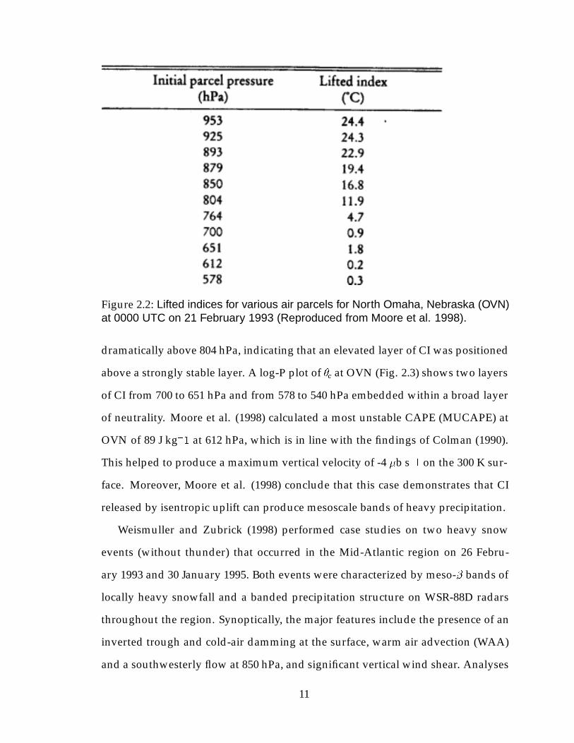
Figure 2.2: Lifted indices for various air parcels for North Omaha, Nebraska (OVN)at 0000 UTC on 21 February 1993 (Reproduced from Moore et al. 1998).

dramatically above 804 hPa, indicating that an elevated layer of CI was positioned

above a strongly stable layer. A log-P plot of �e at OVN (Fig. 2.3) shows two layers

of CI from 700 to 651 hPa and from 578 to 540 hPa embedded within a broad layer

of neutrality. Moore et al. (1998) calculated a most unstable CAPE (MUCAPE) at

OVN of 89 J kg�1 at 612 hPa, which is in line with the findings of Colman (1990).

This helped to produce a maximum vertical velocity of -4 �b s�1 on the 300 K sur-

face. Moreover, Moore et al. (1998) conclude that this case demonstrates that CI

released by isentropic uplift can produce mesoscale bands of heavy precipitation.

Weismuller and Zubrick (1998) performed case studies on two heavy snow

events (without thunder) that occurred in the Mid-Atlantic region on 26 Febru-

ary 1993 and 30 January 1995. Both events were characterized by meso-� bands of

locally heavy snowfall and a banded precipitation structure on WSR-88D radars

throughout the region. Synoptically, the major features include the presence of an

inverted trough and cold-air damming at the surface, warm air advection (WAA)

and a southwesterly flow at 850 hPa, and significant vertical wind shear. Analyses

11

Figure 2.3: T-log P plot of �e (K) at North Omaha, Nebraska (OVN) at 0000 UTC on21 February 1993. (Reproduced from Moore et al. 1998).

of both events show that the heavy snow bands were located within the regions of

the most negative EPV, in which CSI was released by mid-level frontogenesis. This

suggests that these inverted trough-cold air damming scenarios are examples of a

classic warm-frontal CSI scenario, because of the tendency for anticyclonic shear

and large vertical shear to be present with these events.

Similar case studies were examined by Nicosia and Grumm (1999) on three

heavy snow events (4-5 February 1995, 14-15 November 1995, and 12-13 January

1996) in the Mid-Atlantic and Northeastern states. Using Meso Eta Model gridded

data, the two-dimensional Petterssen frontogenesis and saturated equivalent po-

tential temperature (�es) were calculated every three hours for each event. Each cy-

clone exhibited the consistent vertical structure of an evolved cyclone (i.e. stacked),

and produced meso-� bands of heavy snowfall. In each case, the heaviest snow

was observed in bands coinciding with regions of intensifying mid-level frontoge-

nesis and the most negative EPV. CSI was observed in each case, although embed-

12

Figure 2.4: Conceptual model depicting the frontogenetical region and zone of EPVreduction in a developing cyclone (Reproduced from Nicosia and Grumm 1999).

ded regions of CI developed with time on the warm side of the warm frontogenet-

ical region, producing locally intense snow bursts of as much as 6 inches per hour.

The authors speculate that CI in conjunction with CSI may help in the formation

of a multi-banded precipitation structure. Figure 2.4 shows a conceptual model of

a mature cyclone, in which the authors theorize that EPV will be most negative

on the warm side of the mid-level frontogenetical region in the vicinity of the dry

tongue jet (DTJ). At this point, where the cold conveyor belt (CCB) becomes juxta-

posed with the DTJ, the differential moisture advection is the greatest. This leads

to a steepening of �e surfaces while Mg surfaces are unaffected. As a result, EPV is

reduced and may be further reduced by frontogenesis to produce mesoscale bands

(Fig.2.5) As each cyclone became vertically stacked at the end of its development

phase, values of EPV increased as a result of decreased vertical shear and increased

inertial stability. In general, this study suggests that bands of snowfall with accu-

mulation rates of greater than an inch per hour are more likely within deep layers

of highly negative EPV that are intersected by a region of mid-level frontogenesis.

13

Figure 2.5: Proposed positive feedback mechanism between frontogenesis and thereduction of EPV (Reproduced from Nicosia and Grumm 1999).

Perhaps the most extensive study of a single thundersnow event was presented

by Martin (1998a, b). This 19-20 January 1995 event occurred in the Midwest and

was characterized by a 1100-km long, 65-km wide band of snowfall totaling at

least 12 inches (Fig. 2.6). Martin (1998a) attributes the band, which included re-

ports of lightning and thunder (Fig. 2.7), to the interaction of a bent-back front and

a narrow wedge of high �e air, known as the trowal, in the occluded sector of the

cyclone. The bent-back front acted as a warm baroclinic zone and, coupled with

a deformation zone, acted as a source of pronounced frontogenesis. Analysis of

200-m frontogenesis fields shows the process of frontal fracture as time progressed

(Fig. 2.8), in which the warm frontogenetical region to the northwest of the low

center moved farther from the cold frontogenetical region. The warm frontogene-

sis region was the site of the strongest upward vertical velocities, and was nearly

collocated with the region of heavy snowfall. Cross sections of �e and EPV reveal

that weak symmetric stability (WSS) was present in the lower to middle tropo-

sphere over the snowfall region. While a layer of CI was present at the 5-km level,

relative humidities were well below saturation. Therefore, it is very unlikely that

any CI would have been released.

Martin (1999) used ~Q to evaluate quasigeostrophic (QG) forcing within the

trowal airstream. Trajectory analysis of several occluded cyclones shows that the

14

Figure 2.6: Observed 24-hour snowfall totals (cm) ending at 0000 UTC on 20 Jan-uary 1995. (Reproduced from Martin 1998b).

Figure 2.7: Cloud-to-ground lightning strikes in a 24-hour period ending at 0000UTC 20 January 1995 (Reproduced from Martin 1998b).

15

Figure 2.8: (a) 6-hour forecast of 200-m frontogenesis from the UW-NMS modelvalid at 0600 UTC 19 January 1995. Shaded regions denote positive frontogenesisevery 1 K (100 km)�1 day�1. (b) As in (a) except from a 12-hour forecast valid at1200 UTC on the same day. (c) As in (a) except from a 18-hour forecast validat 1800 UTC. (d) As in (a) except from a 24-hour forecast valid at 0000 UTC 20January 1995. (e) As in (a) except from a 30-hour forecast valid at 0600 UTC 20January 1995. (Reproduced from Martin 1998a).

trowal airstream originates in the warm sector and is then cyclonically wrapped to

the north of the low center, acting as a source of significant ascent in the process

and focusing precipitation beneath it. ~Q, which can be used to accurately represent

the QG ! equation, can be divided into its component terms ( ~Qn and ~Qs) (Keyser

et al. 1988) in a natural coordinate system (Fig. 2.9). ~Qn is proportional to the

magnitude of QG frontogenesis and is defined as

~Qn = (~Q � r�

jr�j)n: (2.8)

Positive values of ~Qn convergence (-2r� ~Qn) are indicative of forcing for ascent as a

result of frontal scale processes. ~Qs is representative of the rotation of the thermal

field and the contributions of synoptic scale processes to forcing for ascent (Fig.

2.10). ~Qs is defined as

~Qs =~Q � (k �r�)

jr�j(k �r�

jr�j): (2.9)

16

Figure 2.9: Schematic showing the natural coordinate partioning of ~Q. Dashedlines depict isentropes on an isobaric surface (Reproduced from Martin 1999).

Positive values for the convergence of ~Qs (-2r � ~Qs) are indicative of large-scale

(synoptic scale) forcing for ascent. Martin‘s (1999) analysis of three occluded cy-

clones shows that ascent within the trowal in the occluded sector occurs primarily

due to the convergence of ~Qs (Fig. 2.11), thus indicating synoptic scale QG forcing.

Schultz and Schumacher (SS); (1999) present a comprehensive overview on

many of the concepts and diagnostic methods that relate to symmetric and up-

right instability. Included in this overview is a comprehensive review of defini-

tions of several types of instabilities (Fig. 2.12). (Note that SS uses the term MPV,

not EPV.) The major contention of SS is that �es must be used in order to accurately

diagnose CSI, not �e or �w, because �es assumes that the environment is saturated

everywhere. This includes its insertion into the EPV equation to replace �e, thus

making the term EPV�. Otherwise, SS assert that the use of �e actually diagnoses

potential symmetric instability (PSI). However, we assume that if PSI occurs in a

moist region where the relative humidities are greater than 80 percent (Bennetts

and Sharp 1982) , then it in effect becomes a CSI environment.

17

Figure 2.10: The effect of ~Qs on horizontal thermal structure. (a) Isentropes (solidlines) in a field of ~Q, with the maximum region of convergence shaded. Dashedline indicates convergence axis, while r� depicts thermal gradient. (b) Thick blackarrow depicts original direction of r�, while thick gray arrow depicts the directionof r� after being rotated by ~Qs. (c) Oriention of thermal zone in (a) after beingrotated by ~Qs (Reproduced from Martin 1999).

18

Figure 2.11: (a) Convergence of ~Qs contoured and shaded every 5� 10�16 m kg�1

s�1 in the 600-900 hPa layer from an 18-hour forecast of the UW-NMS model validat 0600 UTC 23 October 1996. (b) As in (a) except for ~Qn (Reproduced from Martin1999).

Figure 2.12: Defintions of several types of instabilities (Reproduced from Schultzand Schumacher 1999).

19

Schultz (1999) also addressed the production of lightning and thunder in lake-

effect snowstorms. His hypothesis is that the generation of lightning is dependent

upon the presence of relatively higher temperatures and dewpoints in the lower

troposphere than those observed in non-thunder producing systems. This may be

because the -10o C isotherm charging region is at sufficient elevation to increase

low-level vertical velocities to point of being able to separate charge.

2.2 Thundersnow-related Climatology

Curran and Pearson (1971) found 76 reports of TS throughout the contiguous United

States for the general time period of 1968 to 1971. After selecting crtieria that a re-

port of TS had to be within 90 nautical miles of a radiosonde station, and that the

report had to be within 3 hours of the time of the sounding, a mean proximity

sounding was constructed for the remaining 13 reports of TS. The mean sounding

(Fig. 2.13) shows that the atmosphere is very moist thoughout the entire depth of

the column. A shallow inversion (81 hPa deep), is located just above the surface.

Just above the inversion from 800 to 600 hPa, the sounding is very close to moist

adiabatic.

Colman (1990) presents the results of a four-year climatology of cold sector, el-

evated thunderstorms, of which thundersnow is a particular type. Colman (1990)

identifies three major factors that facilitate the development of elevated thunder-

storms - a cold upper troposphere, rapid heating and moisture advection near the

boundary layer, and a strongly baroclinic environment. He observed that elevated

thunderstorms are favored to the northeast of a surface cyclone in advance of a

shallow frontal zone, in a region of cyclonic flow at 850 hPa, anticyclonic flow at

500 hPa, and strong vertical shear. Not surprisingly, the mean Showalter Index

(SI) in such events was significantly lower than the mean Lifted Index (LI), 0.6 and

7.4 respectively,, which is indicative of strong inversion layer. One of the most

20

Figure 2.13: Mean proximity sounding for 13 thundersnow reports during the periodof 1968-1971. The thick, solid line depicts the temperature profile. The thick,dashed line depicts the dewpoint profile (Reproduced from Curran and Pearson1971).

21

Figure 2.14: Number of hours of thunder at temperatures below 0� C from 1982-1990. (Reproduced from Holle et al. 1998).

interesting of Colman’s (1990) findings is that elevated thunderstorms frequently

develop in the presence of very small MUCAPE, where the environment is essen-

tially neutral, but in a region of large horizontal stability gradients.

A comprehensive climatology of thundersnow and other types of cold weather

thunderstorms was conducted by Holle et al. (1998), and encompassed the period

of 1982-1990. An examination of Fig. 2.14 shows four preferred regions for the oc-

currence of thundersnow - the Basin and Range province in the southwestern U.S.,

the Central Plains, the Great Lakes region, and coastal regions of the Mid-Atlantic

and New England states. This study suggests that snowfall rates may increase

when accompanied by thunder and lightning, and demonstratively illustrates that

the heavy snowfall is more likely when temperatures fall below 5� C, thus making

the forecasting of thundersnow quite important.

2.3 Summary

In summary, the preceding review points to a strong correlation between the occur-

rence of heavy snow bands and the production of strong ascent by frontogenetical

22

forcing. Thundersnow can be produced when CSI or CI is released by frontogen-

esis, or in the presence of WSS coupled with intense forcing for upward motion.

Thundersnow appears to be favored in two regions - to the north of a warm baro-

clinic zone in association with an open-wave cyclone and southwesterly 700-850

hPa flow (Holle et al. 1998, Weismuller and Zubrick 1998, Nicosia and Grumm

1999) due to the release of CSI, and within the trowal airstream in the northwest or

occluded sector of a mature cyclone (Martin 1998a,b) where no type of instability

has been shown to be preferred.

23

Chapter 3

Methodology

3.1 Climatology

Data in the form of hourly surface airways (SA) observations were obtained from

a CD-ROM of 223 first-order stations in the contiguous United States covering the

period of 1961 to 1990. Software was written to search for all possible combinations

in which thunder and snow were reported simultaneously. These observations of

thundersnow were then separated into three geographical regions (East, Central,

and West) that are outlined in Fig. 3.1. Using the Digital Atmosphere meteoro-

logical software package from WeatherGraphics Technologies, surface maps were

produced for each observation of thundersnow (TS) based on a Barnes analysis

scheme. The reports were then segregated into events using the following criteria

to define an event:

1. Reports of TS at a single station cannot be separated by more than six

hours, or reports from more than one station in the same geographical

region cannot be separated by more than six hours.

2. The report of TS should be within 1100 km of the center of a parent low

(if present), or be within the cloud shield and region of cyclonic flow

around the parent low.

3. If TS was reported by two stations for the same general time period,

24

Figure 3.1: Delineation of regions used in the thundersnow climatology.

then the distance between them must be no more than 1100 km.

(Note: The distance of 1100 km was chosen arbitrarily and is the midpoint between

the low and high ends of the meso-� spatial scale.)

Each event was then referenced according to its initial report of TS, and then

again segregated by the time of day (LST), month, year, intensity of snowfall, geo-

graphical region, temperature, dewpoint, sea level pressure (SLP), wind speed and

direction, and meteorological direction and distance (km) from the parent low. The

direction and distance readings were obtained using a simple screen utility avail-

able with Digital Atmosphere.

Events were then placed into one of the following seven categories:

1. Associated with a surface low with an identifiable position,

2. Lake-effect snow (Great Lakes or Great Salt Lake),

3. Upslope regime,

25

4. General orographic,

5. Associated with a surface low in the Atlantic or Pacific Ocean of uniden-

tifiable position,

6. Associated with a surface low in Mexico, Canada, or the Gulf of Mexico

of unidentifiable position,

7. Miscellaneous or unclassifiable

Categories 2,3,and 4 include events that are not within the cloud shield or wind

flow of a surface cyclone. Category 3 events include those in which the winds were

easterly to southeasterly for most of the stations in the Rocky Mountain region that

surround a particular TS report. Category 4 events tended to have a westerly flow

associated with them.

A state-by-state count of thundersnow events was also conducted. If an event

encompassed several states, such as Oklahoma, Arkansas, and Missouri, then it

was counted as an event for each of those states. However, the event would still be

counted as one in the overall count. The events were also normalized according to

the land area of the average state (61,657.18 mi.2) in the contiguous U.S. as follows:

Va

61; 657:18mi:2(A) = Vn; (3.1)

where Va is the actual number events for a given state, A is the land area for that

state, and Vn is the normalized value for that state.

3.2 Case Studies

Five TS events were examined in depth in order to determine the most significant

reasons for occurrence of thunder. More specifically, each case was examined in

order to determine if any underlying instabilities were present and, if so, what

type. The major forcing mechanisms responsible for enhanced ascent were also

26

identified using isobaric, isentropic, and QG techniques. Even though the goals of

each examination are the same, the methods by which these were accomplished

differed as a result of the types of data that were available on an individual ba-

sis. As a result, the three methods by which the five cases were examined will be

presented in the subsections that follow.

3.2.1 9 December 1999, 11 March 2000, and 19 April 2000

Analyses of these events were accomplished via the use of GEMPAK (GEneral

Meteorological PAcKage) on a Sun Ultra60 UNIX workstation. RUC initial fields

and hourly surface data for the time of the observation of TS were utilized for the

purpose of diagnosing the cause of thunder in each case. The RUC was chosen

because of its mesoscale resolution (40 km on a 151 � 113 grid) and because initial

fields are available on an hourly basis. Also, papers by Schwartz et al. (2000)

and Smith et al. (2000) have revealed that the RUC is quite effective at resolving

parameters that relate to convective activity.

Hourly METAR reports were plotted for the time of TS occurrence, and tem-

perature (every 5� F) and pressure (every 2 hPa) were analyzed using both subjec-

tive and objective means. The objective analysis was accomplished using a Barnes

scheme on a 55 � 55 grid with a 75 km grid spacing. The locations of fronts and

pressure centers were analyzed subjectively and drawn by hand. When possible,

mandatory upper air data (TTAA and TTBB) were plotted for the time of the TS ob-

servation and analyzed both objectively and subjectively. Otherwise, RUC initial

fields were contoured.

Using GEMPAK’s program for vertical interpolations (GDVINT), RUC isobaric

fields were converted into isentropic coordinates, and kinematic omegas were cal-

culated, where

27

� = T (1000

p)RdCp ; (3.2)

and

! = !(pref)�

Zp

pref

(r � ~V )dp: (3.3)

� is the temperature a parcel would possess if it were displaced vertically to 1000

hPa, T is the temperature at the initial pressure level (p), Rd is the dry gas constant,

Cp is the molar heat capacity at constant pressure, and pref is the pressure at some

reference level. pref is usually assumed to be the surface and !(pref ) is usually

assumed to be zero. This method follows that proposed by O’Brien (1970).

Plan view analyses of �e, which is conserved for moist processes, were per-

formed on the mandatory levels in order to locate any possible trowal structures.

�e is expressed as

�e = �LCL exp(Lvrs

CpTLCL); (3.4)

where �LCL is the potential temperature at the lifting condensation level, Lv is the

latent heat of vaporization, rs is the saturation mixing ratio, and TLCL is the tem-

perature at the LCL.

Petterssen surface frontogenesis (=), ~Qs (see Equation 2.8), and ~Qn (see Equa-

tion 2.9) were calculated for each mandatory level in order to diagnose forcing (A

GEMPAK script was written in order to calculate ~Qs and ~Qn), where

= =1

2Cjr�j(E cos 2� �D); (3.5)

and C is a unit conversion (1:08 � 109), E is the total deformation, D is the diver-

gence (r � ~V ), and � is the angle between the axis of diliation and the isentropes.

28

Upper tropospheric influences were ascertained via the analyses of the 300 hPa

divergence fields, while traditional analyses of �a were also performed.

Tropopause-related influences were assessed by the analyses of dynamic tropopause

pressures and the 300-700 hPa potential vorticity in isobaric coordinates, which is

expressed as

PV� = �g[�� + f + (k �@~v

@�)]@�

@p; (3.6)

where �� is the mean layer vorticity.

Cross sections were constructed for = and ! in order to assess the impact of

frontogenetical forcing more directly, and for �, �e, �es, relative humidity (RH), Mg,

and the three-dimensional EPV (EPV3D) to assess stability. When possible, cross

sections were oriented normal to the thermal wind so that the slopes of �e/�es and

Mg could be compared in an assessment of PSI/CSI. However, this is not necessary

when EPV3D is being utilized. EPV3D (see Equation 2.7) was calculated via a GEM-

PAK script that was written to compute EPV3D at 50 hPa increments from the 900

hPa to 200 hPa levels. Regions of PSI (SS) that were located within regions with

RH of greater than 80 percent are assumed to CSI, using the guideline established

by Bennetts and Sharp (1982). If the region of PSI, or any other instability, was lo-

cated within a region in which the RH was less than 80 percent then the instability

was assumed to be untapped, and not a likely contributer to the production of TS.

When possible, stability indices for a nearby sounding (< 50 km from the TS ob-

servation) were examined in order to further assess the possibility of gravitational

instability, otherwise RUC analyses of these parameters (such as the Lifted Index,

Showalter Index, etc.) were contoured from RUC initial fields.

Isentropic analyses of pressure were plotted on isentropic levels along with

storm-relative moisture transport vectors in order to ascertain isentropically-related

vertical motion. A � level was chosen via the examination of cross sections, to de-

29

termine where the RH was greater than 80 percent, and where the vertical motion

was the strongest in a column above the location of the TS observation. Moisture

transport vectors (q~V ) give an indication of not only the flow of moisture, but of

moisture convergence as well. The storm-relative component (~V � ~C) (Moore et

al. 1998) indicates the flow relative to the motion of the system (~C), which was

considered to be the same as the motion of the absolute vorticity maximum that

was associated with the parent cyclone. ~C was calculated as the storm motion over

a period of 6 hours.

3.2.2 5 December 1999

Much of same procedure that was administered in Subsection 3.2.1 was used with

this case. However, because GEMPAK compatible RUC fields were not available,

the PCGRIDDS software package was used instead. The RUC files were obtained

from the National Weather Service Office in Pleasant Hill, Missouri. EPV3D, �es,

and q~v could not be calculated, so a �e-RH-Mg cross section was used to assess

CSI/PSI. Surface analyses were generated using GEMPAK.

30

Chapter 4

Thundersnow Climatology

4.1 Spatial and Temporal Patterns

The search for TS during the period of 1961 to 1990 uncovered 563 reports for the

available data set. Using the criteria previously discussed to identify a TS event,

some 375 were established. While TS events certainly occurred within gaps be-

tween observing stations in the data set, the 30-year period of record establishes

an accurate climatology for the basic synoptic spatial and temporal characteristics

of TS. Of the major regions that were identified in Fig. 3.1, the Central Region

showed the greatest preference for the occurrence of TS with 164 events, while the

East had the fewest (Fig. 4.1).

On a smaller scale, Utah and Nevada showed the greatest preference for TS

occurrence (Fig. 4.2), while secondary areas of preference were observed over the

North Central Plains and the Northeast. While Category 1 type systems were the

most common in all three major geographical regions (Fig. 4.3), there are undoubt-

edly terrain influences that effect TS occurence, especially in the West and East

Regions. Category 3 and 4 events are not uncommon in the West Region, and il-

lustrate the importance of orographic lift to the production of TS in the West. As a

result, it is likely that orography plays a significant role in the production of TS in

Category 1 events as well, especially in the Basin and Range of Utah and Nevada

where mountians are aligned at what are typically high angles to the prevailing

31

Figure 4.1: Number of thundersnow events for each region during the period of1961-1990. Refer to regions depicted in Fig. 3.1.

westerly flow. The presence of large, relatively warm bodies of water (Great Salt

Lake and the Great Lakes) also influence TS occurence in all regions. This is not

only due to pure lake-effect snowstrorms, but lake-enhanced vertical motion in

Category 1 events as well.

A land area-based normalization of the values expressed in Fig. 4.2 reveals a

somewhat different spatial pattern (Fig. 4.4). The primary maximum now shifts to

the eastern seaboard from the Mid-Atlantic to the New England region, although

the values for smaller states, such as Rhode Island and Delaware, are falsely el-

evated due to their extremely small land areas. An analysis of surface maps of

these events reveals that this occurs mainly as a byproduct of intense coastal cy-

clones. The spatial patterns over the Central and West Regions remain largely un-

changed. However, one notable exception is Texas, where normalization reveals a

32

Figure 4.2: Number of thundersnow events for each state during the period of 1961-1990. Note that the sum of the events will not equal 375 (Refer to Section 3.1).

33

Figure 4.3: As in Fig. 4.1 except events (N=375) by category (Refer to Section 3.1for the description of categories).

much smaller value due to its very large land area. It should be noted that nearly

all TS in the state of Texas occurs in the Panhandle, a very small part of the state

as a whole. As a result, the Texas Panhandle should still be considered a preferred

region for the occurence of TS.

Temporally, TS is most common during the month of March in all regions (Fig.

4.5), when synpotic scale sytems are typically the strongest due to strong tempera-

ture gradients and upper tropospheric winds. This preference was the strongest in

the Central Region, where Wisconsin experienced more TS events than any state

for any month (not shown). A weak, secondary temporal maximum was observed

for November and December over the East and West regions. In the East, this is

the peak of the lake-effect snow season, when the Great Lakes remain largely un-

frozen. In the West, this coincides with the transition into the Pacific ‘wet’ season.

The analysis of initiaton times for TS events shows a slight diurnal trend for all re-

gions (Fig. 4.6), in which the majority of events occur between 1200 and 2400 Local

34

Figure 4.4: As in Fig. 4.2 except with normalized values.

Standard Time. There is no clear explanation for this since TS is nearly always a

result of elevated convection, which should not be affected by diurnal heating. TS

also usually occurs in essentially cloudy region with a stable PBL.

4.2 Characteristics of Thundersnow Observations

After the initial observations of TS events were plotted and analyzed, the data

illustrates that TS occurs primarily in the the northeastern or northwestern quad-

rants of a parent cyclone, if present (Fig. 4.7). This is consistent with the earlier

hypothesis of where TS is likely to occur. The initial TS observations occurred at a

mean distance of 471 km from the parent low, and showed by far the greatest fre-

quency at distances of 200 to 600 km from the low (Fig. 4.8). For all initial reports,

the mean temperature was 31.5� F, the mean dewpoint was 28.5� F, the mean sea

level pressure was 1008.1 hPa, and mean wind was from 1� at 14.3 knots. These

35

Figure 4.5: As in Fig. 4.1 except by month (N=375).

Figure 4.6: As in Fig. 4.1 except by Local Standard Time (LST) (N=375).

36

Figure 4.7: Polar plot showing the location of thundersnow events (Category 1)relative to the position of the center of the parent low (N=247). Direction is given inthe traditional meteorological azimuth (degrees) from the postion of the low to theobserving station. Distances are given in km.

values are represented in the station plot in Fig. 4.9. An analysis of snowfall inten-

sity (Fig. 4.10) shows that light snowfall rates are the most common, but moderate

to heavy snow intensities are certainly not uncommon.

37

Figure 4.8: As in Fig. 4.1 except by distance (km) from parent low center of initialreport (N=375).

Figure 4.9: Representative station model for the average initial report for all thun-dersnow events (N=375). Temperature and dewpoint are given in degrees F, thewind speed in knots, and the sea level pressure in hPa. The standard deviation forall parameters is also represented.

38

Figure 4.10: As in Fig. 4.1 except by snowfall intensity of initial report (N=375).

39

Chapter 5

Case Studies

5.1 5 December 1999

5.1.1 Introduction

This event was highlighted by TS at McConnell Air Force Base, Kansas (IAB), oc-

curred at 0600 UTC on 5 December 1999, and included several reports of distant

lightning by stations in south central Kansas. Snowfall of 4 to 10 inches fell within

a 40-mile wide band extending from southwestern Oklahoma to western Iowa.

The RUC 6-hour forecast valid at 0600 UTC included the possibility of convective

precipitation near IAB (not shown).

5.1.2 Surface Analysis

A routine surface analysis for 0600 UTC on 5 December 1999 (Fig. 5.1) indicates a

closed 1009-hPa closed cyclone over east central Missouri. A cold front trails from

the low across southern Missouri across western Arkansas into eastern Texas. A

1038-hPa anticyclone was centered over southeastern Idaho and was pulling very

cold, polar air into much of the Plains and Rocky Mountain Region, and tighten-

ing the pressure gradient across parts of Kansas. Rain showers were observed in

advance of the cold front, while a broad area of warm-frontal type rainfall was oc-

curring from northeastern Missouri into the Great Lakes Region. A narrow band of

snow, including a report of TS at IAB, extended west of the low from southwestern

40

Figure 5.1: Surface analysis valid at 0600 UTC on 5 December 1999. Isobarsdrawn every 2 hPa. Red line depicts cross section line.

Oklahoma into south central Kansas (Fig.5.2).

5.1.3 Upper Air Analysis

An examination of RUC initial fields for the mandatory levels reveals that the sys-

tem still possessed a baroclinic tilt with height, indicating that the cyclone was

still in its developmental stage. The 850-hPa analysis (Fig. 5.3) shows a 1430-m

closed circulation that is centered near the Kansas-Missouri border. Northeast-

erly winds were producing warm air advection (WAA) over south central Kansas,

while cold air advection (CAA) was occurring over nearly all of Oklahoma. At

700 hPa (not shown), the low was centered slightly to the west, over southeastern

Kansas. Again, weak northeasterly flow was producing WAA near IAB. At 500

hPa (not shown), the low was centered near the Kansas-Oklahoma border, not far

from IAB. A vorticity maximum (34 � 10�5 s�1) was positioned over northeastern

41

Figure 5.2: Radar mosaic valid at 0600 UTC on 5 December 1999 (obtained fromthe National Climatic Data Center).

Oklahoma. At 300 hPa (Fig. 5.4), the low (still closed) was centered over south cen-

tral Kansas. A 120-knot jet streak was located over eastern sections of Oklahoma

and Texas, placing IAB under the left exit region of a curved jet streak, and under

an axis of maximum 300-hPa divergence (Fig. 5.5) in which the highest values (9 �

10�5 s�1) were found to be over eastern Kansas. Therefore, upper tropospheric di-

vergence was likely a very significant factor in the production of ascent near IAB.

Concurrently, significant convergence (-8 � 10�5 s�1) was occurring in the lower

troposphere (not shown), helping to further enhance upward vertical motion by

the process of Dyne’s compensation.

5.1.4 Isentropic Analysis

Analysis of �e contours for the 0600 UTC RUC initial field shows a well defined

trowal structure at the 700-hPa level (Fig. 5.6) that extends from Missouri into

42

Figure 5.3: 850-hPa Rapid Update Cycle initial field analysis valid at 0600 UTC on5 December 1999. Isotherms (thick lines) drawn every 4� C, height contours (thinlines) every 2 dkm.

Figure 5.4: As in Fig. 5.3 except for 300-hPa level. Height contours (thick lines)drawn every 5 dkm, isotachs (thin lines) every 10 knots (2=20 kts, 12=120 kts, etc.

43

Figure 5.5: As in Fig. 5.3 except for 300-hPa divergence (depicted every 2 � 10�5

s�1).

south central Kansas. This feature is poorly defined at 850 hPa and is completely

absent at 500 hPa. However, this is not surprising since the dynamic tropopause

had descended to near the 500-hPa level (Fig. 5.7). As a result, the 500-hPa analy-

sis will be reflective of the intrusion of cold stratospheric air into the middle tropo-

sphere. Also, cyclonic potential vorticity advection will contribute to the formation

of the trowal below the tropopause, as kinetic energy is created and the flow be-

comes more meridional (Hoskins et al. 1985). Also, if Martin’s (1999) assertion that

occlusions may occur from the top down is correct, then the trowal will develop

at the 700-hPa level before it does at 850 hPa. In any event, the close alignment

of the 700-hPa trowal feature and orientation of precipitation echoes (Fig. 5.2) is

indicative that the trowal was the major feature in the production of TS at IAB.

44

Figure 5.6: As in Fig. 5.3 except for 700-hPa equivalent potential temperature(depicted every 2 K).

991205 0600UTC Tropopause P re s su re ( hPa )

150

200

200

200

200

200

200

200

200

200

200

250

250

300

300

350

400

400

450

500

Figure 5.7: As in Fig. 5.3 except dynamic tropopause pressures (depicted every 50hPa).

45

5.1.5 Stability Analysis

A �e-Mg-RH cross-section (Fig. 5.8) was constructed perpendicular to the 0600 UTC

RUC initial field 1000-500-hPa thickness analysis (not shown) from near Dodge

City, Kansas, to near Reelfoot Lake in northwestern Tennessee. While IAB was

located within a deep layer of high RH (>90%), the �e contours are nearly hori-

zontal, indicating that the atmosphere was neither symmetrically nor convectively

unstable. However, an analysis of the lifted index for the 850-700-hPa layer (Fig.

5.9 shows values slightly below zero. As a result, some weak elevated gravita-

tional instability was present over IAB, which could have easily been released by

the abundant middle to upper tropospheric forcing (see next section) that was oc-

curring. Also, the analysis of the RUC initial fields shows that the K-index was

18, and the total totals index was near 44, both indicative of a marginally unstable

atmosphere.

5.1.6 Quasigeostrophic Forcing

The analysis of ~Qs (Fig. 5.10) and ~Qn (Fig. 5.11) at 0600 UTC in the 850-400-hPa

layer shows nearly equal amounts of convergence of quantity (5-10 � 10�19 Pa�1

m�2 s�1) over eastern Kansas. ~Qs convergence is indicative of the reorientation of

the thermal field and synoptic-scale forcing (Martin 1999), and is important to the

formation of the trowal feature. In this case, ~Qs convergence likely results from

strong upper tropospheric influences and potential vorticity conversion related to

the tropopause anomaly. ~Qn convergence is indicative QG frontogenetical forcing

within the trowal feature itself. Therefore, these two major mechanisms of forcing

acted in tandem to release the weak upright instability that was present over IAB.

46

Figure 5.8: Vertical cross section analysis of the 0600 UTC Rapid Update Cycleinitial field from 5 December 1999. Equivalent potential temperature (dashed lines)are depicted every 3 K, Mg (solid lines) depicted every 5 kg m s�1, and relativehumidity (dotted lines) depicted every 5% for values > 80%. KIAB is located near97.25� W longitude.

5.1.7 Conclusions

The TS in this event occurred within the trowal of an occluding cyclone. The trowal

is a region of significant frontogenesis, and is mainly the byproduct of tremendous

amounts of synoptic-scale forcing. With these two forcing mechanisms working

in tandem, and with large amounts of upper tropospheric divergence, this would

easily be sufficient to release small amounts of upright instability and thus create

updraft speeds sufficient to create charge separation. The meso-� banding of the

snowfall observed with this event is common to this type of synoptic setting, and

is largely a byproduct of the orientation of the trowal and frontogenesis fields.

47

Figure 5.9: As in Fig. 5.3 except lifted indices for the 850-700-hPa layer (depictedevery 1� C).

Figure 5.10: As in Fig. 5.3 except for divergence of ~Qs in the 850-400-hPa layer (de-picted every 5 � 10�19 Pa�1 m�2 s�1). Dashed lines depict areas of convergence,while solid lines depict divergence.

48

Figure 5.11: As in Fig. 5.10 except for divergence of ~Qn.

5.2 9 December 1999

5.2.1 Introduction

This event featured a 99-minute episode of thunderstorms with sleet, that was

mixed with snow at times, at Lubbock, Texas (LBB) that occurred at approximately

0900 UTC on 9 December 1999. Snow and sleet accumulation at LBB totaled 7

inches in a 5-hour period, although much of that fell after the thunderstorms had

ended. Surface observations of in-cloud and cloud-to-cloud lightning were com-

mon at LBB just before and at the onset of precipitation at 0917 UTC.


At 0900 UTC on 9 December 1999, the surface analysis (Fig. 5.12) shows a 1010-hPa

closed surface cyclone over north central Texas, not far from the Dallas-Ft. Worth

metroplex. A cold front trails from the low across south central Texas and then

into Mexico. At this time, snow is limited to the northern Texas Panhandle, while

a more broad area of rain and thunderstorms was extending from Oklahoma into

49

Figure 5.12: Surface analysis valid at 0900 UTC on 9 December 1999. Isobarsdepicted every 2 hPa. Red line depicts cross section line.

west central Missouri along a warm front (Fig. 5.13). A sharp temperature contrast

is observed across Texas, where temperatures were in the upper sixties (�F) over

central and southern portions of the state, but only in the upper twenties and thir-

ties in the west (Fig. 5.12). A 1030-hPa anticyclone is centered over northwestern

Colorado, pulling very cold Polar air into the Plains and Rocky Mountain regions.


The RUC initial analysis valid at 0900 UTC shows a 1460-m 850-hPa low over

northwestern Texas (Fig. 5.14). As a result, WAA is occurring over most of the Pan-

handle region, while CAA is occurring over the remainder of the western Texas.

A 3020-m low is indicated at the 700-hPa level (not shown), with its center being

located just to the south of LBB and its circulation again producing WAA over the

Panhandle. At 500 hPa, a 5560-m low is centered along the Texas-New Mexico

border, while a vorticity maximum (38 � 10�5 s�1) is located just to the east of the

50

Figure 5.13: Radar mosaic valid at 0900 UTC on 9 December 1999 (obtained fromthe National Climatic Data Center).

500-hPa low center (Fig. 5.15). The 300-hPa initial field analysis shows a 90-knot

jet streak emerging from the base of a trough over western Texas (Fig. 5.16), plac-

ing LBB in a region of weak divergence (2 � 10�5 s�1). Analysis of the dynamic

tropopause shows a 500-hPa tropopause anomaly (Fig. 5.17) near the location of

the 500-hPa low (Fig. 5.15), which is associated with a 25 � 10�7 K m�1 Pa�1 s�3

potential vorticity maximum located near the position of the 500-hPa low center.


An isentropic pressure analysis of the 294 K surface (from the 0900 UTC RUC initial

field) shows a well-defined trowal feature that originates over southern Texas and

then wraps cyclonically into the Texas Panhandle and northeastern New Mexico

(Fig. 5.18). An analysis of storm-relative moisture transport vectors (Fig. 5.18)

shows that the flow of moisture is oriented very closely to the alignment of the

51

991209/0900V000 850 MB HGHT

1470

1500

1500

1530

1530

1530

1530

1560

1560

991209/0900V000 850 MB TMPC

-5

-5

-5

-5

0

0

5

5

1010

15

Figure 5.14: 850-hPa Rapid Update Cycle initial field analysis valid at 0900 UTC on9 December 1999. Isotherms (dashed lines) contoured every 5� C, height contours(solid lines) every 30 m.

991209 /0900V000 500 MB HGHT

5580

5580

5580

5640

5700

5760

5820

991209 /0900V000 500 MB AVORWND (*10**5 )

0

5

5

5

5

55

5

5

5

10

10

10

10

10

15

15

2025

30

35

Figure 5.15: As in Fig. 5.13 except 500-hPa heights and absolute vorticity. Absolutevorticity (dashed lines) contoured every 5 � 10�5 s�1, height contours (solid lines)every 60 m.

52

991209 /0900V000 300 MB MULSPED1 .94

30

50

50

5070

70

7 0

70

70

90

90

90

90

110

991209 /0900V000 300 MB HGHT

9120

9240

9360

9480

9 4 8 0

991209 /0900V000 300 MB DIVWND (*10**5 )

-6

-6

-6

-6

-6

-6

-4

-4

-4

-4

-2

-2

-2

-2

-2

-2

0

0

0

0

0

0

00

2

22

2

2

2

2

2

4

4

4

6

6

6

Figure 5.16: As in Fig. 5.13 except 300-hPa heights, divergence and isotachs.Isotachs (solid purple) contoured every 20 knots and shaded for speeds > 70knots, height contours (solid black) every 120 m, and divergence (dashed red)every 2 � 10�5 s�1.

991209 /0900V000 SFC PRES

150

150

150

150

200

200

2 0 0

200

2 0 0

2 5 0

2 5 0250

250

250

300

350

400450500

9 9 1 2 0 9 /0 9 0 0 V0 00 300 : 700 MB PVORTHTA (*10**7 )

0

5

5

5

10

15

15

20

25

Figure 5.17: As in Fig. 5.13 except dynamic tropopause pressure and 700-300-hPapotential vorticity. Isobars (solid) depicted every 50 hPa, potential vorticity (dashed)every 5 � 10�7 m2 K s�1 kg�2.

53

991209/0900V000 294 K PRES

600

650

700

750

750

800

850900 950

950

SR-MTVEC

100. m/s

Figure 5.18: As in Fig. 5.13 except pressure and storm-relative moisture transportvectors on the 294 K isentropic surface. Isobars (solid) depicted every 50 hPa,vectors indicate storm-relative moisture transport (q(~V � ~C)). ~C calculated to befrom 257� at 13.7 m s�1.

trowal, which suggests that the trowal airstream was not only the major supplier

of Gulf moisture to the system, but was the principle source of isentropic uplift.

Isentropic uplift was the strongest over the Texas Panhandle where the pressure

gradient is strongest, and where the trowal airstream was forced upward over the

warm baroclinic zone.

5.2.5 Stability and Forcing

A cross section constructed from Clovis, New Mexico (CVS), to Dallas-Ft. Worth

International Airport, Texas (DFW), shows a layer of elevated CI (Fig. 5.19) that

spans the entire length of the cross section, and extends from near 750 hPa to 550

hPa above LBB. This layer of CI begins near the top of a layer of high RH (>80%)

that extends from the surface to 700 hPa. So, there would have been adequate

moisture for the release of CI to produce TS.

54

200

250

300

350

400

450

500

550

600

650

700

750

800

850

900950

CVS DFW

80

90

991209/0900V000 RELH

292 294296 298

300302304

304

306308

310

312

312

314

314

316

316

318

318

320

320

322

322

324

324

326

326

328

328

330332334

336338340

342344346348350352

354

991209/0900V000 THTE

200

250

300

350

400

450

500

550

600

650

700

750

800

850

900950

CVS DFW

-20

-10

0

10

20

30 40 50 60

70

80

80

90

991209/0900V000 MSFC

200

250

300

350

400

450

500

550

600

650

700

750

800

850

900950

CVS DFW

Figure 5.19: Vertical cross section from Clovis, New Mexico (CVS), to Dallas-Ft.Worth, Texas (DFW), from the 0900 UTC RUC initial field valid on 09 December1999. Solid lines depict equivalent potential temperature (every 2 K), dashed linesdepict absolute geostrophic momentum (every 10 kg m s�1). Values of relativehumidity greater than 80% are shaded green, and greater than 90% dark green.LBB is located near the second tick mark from the left edge.

55

- 10

-9

-9

-8

-8

-7

-6

-5

-5

-5

-4

-4

-4

-3

-3

-3

-2

-2-2

-1

-1

0

0

0

991209 /0900V000 OMEG (*10**3 )

1 0 0

1 5 0

2 0 0

2 5 0

3 0 0

3 5 0

4 0 0

4 5 0

5 0 0

5 5 0

6 0 0

6 5 0

7 0 0

7 5 08 0 08 5 09 0 09 5 0

CVS DFW

-28-24-20 -16-12

-8

-8

-8

-4

-4

-4

-4

-4

0

0

0

0

0

0

4

44

4

4

4

4

8

8

8

12

1 2

1 21 6202 42 83 2

9 9 1 209 /0900V000 FRNTTHTAUOBS (*10**1 )

1 0 0

1 5 0

2 0 0

2 5 0

3 0 0

3 5 0

4 0 0

4 5 0

5 0 0

5 5 0

6 0 0

6 5 0

7 0 0

7 5 08 0 08 5 09 0 09 5 0

CVS DFW

Figure 5.20: As in Fig. 5.18 except Petterssen surface frontogenesis (solid lines,every 4 � 10�1 K 100 km�1 3 h�1), and ! (dashed lines, every 3 �b s�1.

Figure 5.20 shows that upward vertical motion was the strongest (-10 �b s�1) at

the 450-hPa level above LBB. A second axis of strong vertical motion was located

near the 725-hPa level. Each of these regions of strong upward motion are associ-

ated with corresponding regions of frontogenetical maximums at the same levels

(Fig. 5.20). The region of frontogenesis in the lower troposphere is associated with

the trowal feature, while the region in the middle troposphere is associated with

the intrusion of very cold stratospheric air in the tropopause fold. This suggests

that these two regions of frontogenesis acted in tandem to release CI, and to en-

hance upward vertical motion.

The computation and analysis of ~Qs and ~Qn convergence for the 850-400-hPa

layer above LBB (Figs. 5.21 and 5.22, respectively) shows values of 6 � 10�14 m

kg�1 s�1 and 3 � 10�14 m kg�1 s�1, respectively. A level-by-level analysis of ~Qs

and ~Qn convergence shows that ~Qs convergence was the strongest at 500 hPa, at

the height of the tropopause anomaly, and was positive for all points above the

56

9 9 1 2 0 9 (1200V00) 400 :850 Laye r Qs Conve rgence

-8

-4

-4-4

0

0

0

0

0

0

0

0

4

812

16

20

Figure 5.21: As in Fig. 5.13 except convergence (positive values) of ~Qs in the850-400-hPa layer. Contours drawn every 4 � 10�14 m kg�1 s�1.

850-hPa level (not shown). Meanwhile, ~Qn convergence was strongest at the 850-

hPa level (not shown). This suggests that large-scale processes were primarily

responsible for ascent in this case, as well as for the production of the frontogenesis

fields that acted as releasing mechanisms for CI.

While EPV3 was analyzed (Fig. 5.23), it cannot be used as a diagnostic tool

for CSI in this case because the atmosphere is not convectively and gravitationally

stable. Although a large area of negative EPV3 is evident, it is only indicative that

some type of instability is present (Moore and Lambert 1993). A comparison of

cross sections of EPV3 that were calculated using �e (Fig. 5.23) and �es (Fig. 5.24)

shows that the two are nearly identical. Therefore, either method would have

worked well in this case study.

57

9 9 1 2 0 9 (1200V00) 400 :850 Laye r Qn Conve rgence

-5

-4

-3

-2

-2

-2

-1

-1-1

-1

-1 -1

-1

-1

-1

-1

-1

-1

-1

0

0

0

0

0

0

0

0

0

0

1

1

1 1

1

1

1

1

1

1

2

2

2

2

3

45

Figure 5.22: As in Fig. 5.20 except convergence (positive values) of ~Qn in the850-400-hPa layer. Contours drawn every 1 � 10�14 m kg�1 s�1.

-3-2

-1

-1

0

0

0

1

1

1

2

22

3

3

3

4

4

56

991209/0900V000 EPV3 (*10**6)

200

250

300

350

400

450

500

550

600

650

700

750

800

850

900950

CVS DFW

Figure 5.23: As in Fig. 5.18 except three-dimensional equivalent potential vorticitycalculated with �e. Contoured every 1 PVU with negative values shaded.

58

-1

0

0

0

1

1

1

2

22

3

3

33

4

4

56

991209/0900V000 EPVTHES3 (*10**6)

200

250

300

350

400

450

500

550

600

650

700

750

800

850

900950

CVS DFW

Figure 5.24: As in Fig. 5.18 except three-dimensional equivalent potential vorticitycalculated with �es. Contoured every 1 PVU with negative values shaded.

5.2.6 Conclusions

The convective episode associated with this event occurred as elevated CI was

released by frontogenesis. Frontogenesis occurred in the lower troposphere in

association with the trowal, and in the middle troposphere in association with a

tropopause anomaly and its associated stratospheric air intrusion. The two work-

ing in tandem helped to create strong ascent, and ideal conditions for the release

of elevated upright instability.

There can be little doubt that the presence of the tropopause anomaly was also

important in the forcing for upward vertical motion. First, the intrusion of strato-

spheric air would act to lift the warmer, tropospheric air ahead of it, because the

stratospheric air is more dense; this is verified by the frontogenesis fields. Sec-

ondly, the low static stability associated with the anomaly would enhance the po-

tential for stronger upward vertical velocities (Hoskins et al. 1985). Thirdly, large

amounts of kinetic energy would be added to the system, due to conservation po-

tential vorticity, causing the flow to become

59

more meridional (Hoskins et al. 1985). The latter would be important in the cre-

ation of the trowal airstream.

5.3 11 March 2000

5.3.1 Introduction

This event featured numerous reports of TS throughout the greater St. Louis (STL)

metropolitan area, and lightning imagery (not shown) indicates that a band of TS

extended as far south as the Cape Girardeau, Missouri, area. Snowfall totals (not

shown) ranged from 4 to 10 inches (10-25 cm) in a band from central Missouri into

the St. Louis area.


The surface analysis at 1300 UTC on 11 March 2000 (Fig. 5.25) indicates a mod-

est, 1010-hPa closed cyclone over middle Tennessee. A warm front extends to the

east of the low while a cold front trails to the south of the low. A broad area of

rain and snow with embedded thunderstorms is wrapping around the backside of

the low center, while showers and thunderstorms are located in the warm-sector

(Fig. 5.26). A broad anticyclone (1030 hPa) was centered over extreme western

Kansas, and was helping to create a tight pressure gradient and strong winds in

the northwest-sector of the cyclone (Fig. 5.25).


Analyses of the 1200 UTC RUC initial fields on 11 March 2000 shows a closed

850-hPa low circulation over southeastern Missouri (Fig. 5.27). At this time TS is

beginning at STL and weak WAA is occurring at 850-hPa over STL. A closed 700-

hPa low is centered over south central Missouri, while a cold pool is forming over

southwestern Missouri (not shown). A 500-hPa short wave trough extends along

60

Figure 5.25: Surface analysis valid at 1200 UTC on 11 March 2000. Isobars de-picted every 2 hPa. Red line depicts cross section line.

an axis from southwestern Missouri into Louisiana (Fig. 5.28), and its associated

vorticity maximum is positioned over central Arkansas. At 300-hPa, a 100-knot jet

streak was located over southern Arkansas (Fig. 5.29) was helping to produce a

divergence axis (7 � 10�5 s�1) over eastern Missouri (Fig. 5.29). This divergence

axis is nearly colocated with a band of heavier precipitation (Fig. 5.26). In addition,

a slightly elongated tropopause anomaly (450 hPa) and its associated PV anomaly

are located over central Arkansas (Fig. 5.30).


Plan view view analyses of �e from the 1200 UTC RUC initial field indicates that

only a very weak �e ridge is present at 850 hPa (not shown). However, a hint of

a trowal feature is developing at 700 hPa (not shown) and a CAA-WAA couplet

has developed. The trowal feature is significantly better organized at 500 hPa (Fig.

61

Figure 5.26: Radar mosaic valid at 1200 UTC on 11 March 2000 (obtained from theNational Climatic Data Center).

000311 /1200V000 850 MB TMPC

-10

-5

0

0

0 0

05

10

10

000311 /1200V000 850 MB HGHT

1440

1440

1470

1500

1500

1530

1 5 3 0

1 5 6 0

Figure 5.27: 850-hPa analysis of the 1200 UTC Rapid Update Cycle initial fieldvalid on 11 March 2000. Heights (solid,black) depicted every 30 m, temperatures(dashed,red) every 5� C.

62

000311 /1200V000 500 MB HGHT

5400

5460

5520

5580

5640

000311 /1200V000 500 MB AVORWND (*10**5 )

05

5

5

5

5

510

1 0

10

10

10

10

1 0

15

15

1 5

1 5

15

20

25

30

35

Figure 5.28: As in Fig. 5.27 except 500-hPa analysis. Heights (solid,black) depictedevery 60 m, absolute vorticity (dashed, green) every 5 � 10�5 s�1.

000311 /1200V000 300 MB MULSPED1 .94

30

5 0

50

5070

70

90

90

110

000311 /1200V000 300 MB HGHT

8880

9000

9120

9240

000311 /1200V000 300 MB DIVWND (*10**5 )

-4

-4

-4

-4

-2

-2

-2

-2

-2

-2

-2

-2

0

0

0

0

00

0

0

0

2

2

2

2

2

4

4

4

4

4

4

4

6

6

Figure 5.29: As in Fig. 5.27 except 300-hPa analysis. Heights (solid,black) depictedevery 120 m. Isotachs (dashed, purple) depicted every 20 knots with speeds ofgreater than 70 knots shaded. Divergence (dashed, red) depicted every 2 � 10�5

s�1.

63

Tropopause Heights (hPa)

200200

200

200

250

250

300

300

300

300

350

350

400 450

000311/1200V000 300 : 700 MB PVORTHTA (*10**7)

5

55

5 5

10

10

10

15

20

25

Figure 5.30: As in Fig. 5.27 except dynamic tropopause and 700-300-hPa potentialvorticity analyses. Tropopause pressures (solid, black) depicted every 50 hPa,potential vorticity (dashed, red) every 5 � 10�7 m2 K s�1 kg�2.

5.31) where the �e ridge is nearly enclosing the cold air pool. The trowal feature

at this level also closely matches the precipitation field (Fig. 5.26). An analysis

of the 294 K isentropic surface, which was chosen because it is at the level of the

strongest frontogenesis (to be discussed), and moisture transport vectors shows

that significant isentropic upglide is occurring over the STL region (Fig. 5.32), with

the vectors intersecting the isobars at nearly perpendicular angles.


A cross section was constructed from Omaha, Nebraska (OMA), to Atlanta, Geor-

gia (ATL). Figure 5.33 shows that a deep layer of high RH is located above STL

and over locations to the southeast. No instability, either upright or slantwise, is

shown above STL, although CSI is present southeast of STL and convective insta-

bility is present still further southeastward (Fig. 5.33). The three-dimensional EPV

analysis shows that values above St. Louis are less than 1 PVU near the 700-hPa

level (Fig. 5.34), which is indicative that WSS is present. As in the 9 December 1999

64

000311 /1200V000 500 MB THTE

300

302

304

306308 310

312314

316

316

316

3 1 6

318318

Figure 5.31: As in Fig. 5.27 except 500-hPa equivalent potential temperature (de-picted every 2K).

SR-MTVEC000311 /1200V000 294 K PRES

600

650

650

700

750

800850

900

950

Figure 5.32: As in Fig. 5.27 except pressure (depicted every 50 hPa) and storm-relative moisture transport vectors (q(~V � ~C)) on the 294 K isentropic surface. ~C

calculated to be from 293� at 9.3 m s�1.

65

80

80

80

90

90

90

100

150

200

250

300

350

400

450

500

550

600

650

700

750800850900950

OMA ATL

80

90

000311 /1200V000 RELH

0

10

20

30 40 5060 70

70

8090 100

110

120

130

000311 /1200V000 MSFC

100

150

200

250

300

350

400

450

500

550

600

650

700

750800850900950

OMA ATL

278280 282 284286288290292294

296298

300

302

304

306

308

310312

314

314

316

316

318

318

318

318

320

322

324326328

330332334336338340342344346348350352354356358360362364366368370372374376

000311 /1200V000 THTE

100

150

200

250

300

350

400

450

500

550

600

650

700

750800850900950

OMA ATL

Figure 5.33: Vertical cross section from Omaha, Nebraska (OMA), to Atlanta, Geor-gia (ATL), from the 1200 UTC RUC initial field valid on 11 March 2000. Solid linesdepict equivalent potential temperature (every 2 K), dashed lines depict absolutegeostrophic momentum (every 10 kg m s�1). Values of relative humidity greaterthan 80% are shaded green, and greater than 90% dark green. STL is locatedbetween the fifth and sixth tick marks from the left edge.

case, a comparison of the EPV fields using �e (Fig. 5.34) and �es (Fig. 5.35) are very

similar.

Figure 5.36 shows that frontogenesis is occurring at 700 hPa (� 3 � 10�1 K

100 km�1 3 h�1) and rather vigorous upward vertical motion (! � -8 �b s�1) is

occurring above the axis of strongest frontogenesis.

Figures 5.37 and 5.38 show that the layer-average convergence of both QG forc-

ing components were quite weak (2 and 1 � 10�14 m kg�1 s�1, respectively), al-

though ~Qs forcing was slightly greater. The alternating convergence-divergence

patterns in 5.37 are similar to the gravity wave signature discussed by Barnes et al.

(1996). Jewett et al. (2001) point out that gravity waves may help in the formation

66

0

0

0

1

1

11

1

2

2

22

3

3

4

4

5

56

6

6

67

7

7

7

8

8

9

9

10

10

11

11

12

12

13

14

15

000311/1200V000 EPV3 (*10**6)

200

250

300

350

400

450

500

550

600

650

700

750

800

850

900950

OMA ATL


0

0

0

1

1

1

11

2

2

22

3

3

4

4

5

5

6

6

67

7

7

7

8

8

9

9

10

10

11

11

12

12

13

14

15

000311/1200V000 EPVTHES3 (*10**6)

200

250

300

350

400

450

500

550

600

650

700

750

800

850

900950

OMA ATL


67

- 14

-13-12-11

-10-9 -8

-7

-6-5 -4-3

-2-2-1

-10

0

0

0

0

0

0

0

1

1

2

2

3

000311 /1200V000 OMEG (*10**3 )

1 0 0

1 5 0

2 0 0

2 5 0

3 0 0

3 5 0

4 0 0

4 5 0

5 0 0

5 5 0

6 0 0

6 5 0

7 0 0

7 5 08 0 08 5 09 0 09 5 0

OMA ATL

-20

-18

-18

-16

-16

-14

-14

-14

-12

-12

-12

-10

-10

-10

-8

-8

-6

-6-6

-6

-6

-4

-4

-4

-4

-4

-4

-2

-2

-2

-2-2

-2

0

0

0

0

0

0

0

0

0

0

0

0

2

2

2

2

2

2

22

2

4

4

4

4

4

6

6

6

6

8

8

8

10

10

12

1214

16202224

0 0 0 311 /1200V000 FRNTTHTAUOBS (*10**1 )

1 0 0

1 5 0

2 0 0

2 5 0

3 0 0

3 5 0

4 0 0

4 5 0

5 0 0

5 5 0

6 0 0

6 5 0

7 0 0

7 5 08 0 08 5 09 0 09 5 0

OMA ATL

Figure 5.36: As in Fig. 5.33 except Petterssen surface frontogenesis (solid lines,every 2 � 10�1 K 100 km�1 3 h�1), and ! (dashed lines, every 1 �b s�1.

of convective cells by lowering static stability and increasing upward vertical ve-

locities. Therefore, gravity waves may have helped in the production of TS in this

case, although an attempt to show this, conclusively, would be beyond the scope

of this thesis.

5.3.6 Conclusions

The TS that occurred across the STL region on the morning of 11 March 2000 oc-

curred primarily as a result of 700-hPa frontogenesis under conditions of WSS.

Frontogenesis occurred at 700 hPa with the development of an early trowal struc-

ture, which was better organized at 500 hPa. Again, this is suggestive that occlu-

sions may occur from the top-down (Martin 1999). Additional enhancement for

ascent was supplied in the form of upper tropospheric divergence, as the STL re-

gion was under the left exit region of a curved jet streak. The precipitation patterns

coincide very well with the orientation of the trowal, suggesting that the processes

68

0 0 0 3 1 1 /1 2 f00 400 :850 Conve rgence o f Qs (10e -14 )

-12

-10-8

-6

-4

-4

-4

-4

-2

-2

-2

-2

0

0

0

0

0

0

00

0

2

2

2

4

6

8 1012

14 16

Figure 5.37: As in Fig. 5.27 except convergence (positive values) of ~Qs in the850-400-hPa layer. Contours drawn every 2 � 10�14 m kg�1 s�1.

0 0 0 3 1 1 /1 2 f00 400 :850 Conve rgence o f Qn (10e -14 )-5-4-3

-2-2

-2

-1

-1

-1

-1

0 0

0

0

0

1

1

1

2

4

5

Figure 5.38: As in Fig. 5.37 except convergence (positive values) of ~Qn in the850-400-hPa layer. Contours drawn every 1 � 10�14 m kg�1 s�1.

69

that are involved in the generation of the trowal airstream are the same processes

responsible for creating conditions that are favorable for TS.

5.4 19 April 2000

5.4.1 Introduction

The TS in this event occurred at Ellsworth Air Force Base, South Dakota (RCA), on

19 April 2000 at 1200 UTC. The TS occurred as part of a very intense spring storm

that produced blizzard conditions over western South Dakota and severe weather

over portions of the northern and central Plains. Snowfall amounts of over 30

inches (75 cm) were observed to the west of Rapid City, South Dakota (Fig. 5.39).

24-hour snowfall (18.7 in.) and precipitation (3.87 in.) records were set at RCA, as

well as for several other locations in the region. It should be noted that most of the

snow fell in less than a 12-hour period.


The surface analysis at 1200 UTC on 19 April 2000 shows a tightly wound occluded

cyclone along the South Dakota-Nebraska border (Fig. 5.40). An occluded front

extends from the low to the triple point in extreme southwestern Iowa. A warm

front extends across southern Iowa, while a cold front is cutting through eastern

Kansas. A band of locally heavy precipitation, including thunderstorms, extends

from western South Dakota into southern Minnesota (Fig. 5.41). The RCA area is

on the edge of an area of heavy precipitation, which is in the form of TS at this

time.


Analyses of 1200 UTC RUC initial fields on 19 April 2000 indicate that 850 and

700 hPa closed cyclonic circulations (Fig. 5.42) are stacked on top of the surface

70

Figure 5.39: Storm total snowfall amounts (inches) for 19 April 2000. (Obtainedfrom the National Weather Service forecast office in Rapid City, South Dakota.)

Figure 5.40: Surface analysis valid at 1200 UTC on 19 April 2000. Isobars depictedevery 2 hPa. Red line depicts cross section line.

71

Figure 5.41: Radar mosaic valid at 1200 UTC on 19 April 2000 (obtained from theNational Climatic Data Center).

low (Fig. 5.40), which is indicative of a mature, occluded system. The correspond-

ing thermal structure also indicates that the system is occluded. The 500-hPa low

is centered over the Nebraska Panhandle (Fig. 5.43) while a strong vorticity maxi-

mum (40� 10�5 s�1) is positioned just west of the barotropic circulations below. At

300 hPa, an elongated jet streak is emerging from a trough over the southwestern

U.S. (Fig. 5.44). A divergence axis extends from southwestern Iowa into north-

western South Dakota and then into southeastern Wyoming (Fig. 5.44) at the nose

of and in the left exit region of the jet streak. A very elongated dynamic tropopause

fold extends from Utah into South Dakota (Fig. 5.45), with the lowest tropopause

pressures (600 hPa) located over northwestern Nebraska.

72

000419 /1200V000 850 MB HGHT

1320

1350

1380

1410

1 440 1440

1470

1 4 7 0

1 5 0 0

000419 /1200V000 700 MB HGHT

2880

2910

2940

2970

2970

3000

3000

3000

3030

3 0 3 03 0 3 0

3060

Figure 5.42: 850-hPa and 700-hPa RUC initial fields valid at 1200 UTC on 19April 2000. 850-hPa heights (solid, black) depicted every 30 m, 700-hPa heights(dashed, red) depicted every 30 m.

0 0 0419 /1200V000 500 MB AVORWND (*10**5 )

5

5

5

10

10

10

1 0

1010 10

10

10

1520

25

25

30

30

35

40

000419 /1200V000 500 MB HGHT

5460

5520

5520

5640

5 6 4 0

5700

5760

Figure 5.43: As in Fig. 5.42 except 500-hPa analysis. Heights (solid, black) de-picted every 60 m, absolute vorticity (dashed, red) depicted every 5 � 10�5 s�1.

73

000419 /1200V000 300 MB MULSPED1 .94

30

30

50 50

50

50

50

70

70

9 0 110

000419 /1200V000 300 MB HGHT

8880

9000

9120

9120

9240

9360

9480

-6

-4

-4

-4

-2

-2

-2

-2 -2

-2

-2

-2

-2

-2

-2

-2

-2 -2

-2

-2-2

-2

-2

0 0

0

0

0

00

0

0

0

00

0

0

00

0

2

2

2

2

2

22

2

2

2

4

4

44

4

4

6

6

6

8

Figure 5.44: As in Fig. 5.42 except 300-hPa analysis. Heights (solid,black) depictedevery 120 m. Isotachs (dashed, purple) depicted every 20 knots with speeds ofgreater than 70 knots shaded. Divergence (dashed, red) depicted every 2 � 10�5

s�1.

Tropopause He igh t s ( hPa )

150

200

2 0 0250

250

250

300

300

350

450

500

500

550600

0 0 0 4 1 9 /1200V000 300 : 700 MB PVORTHTA (*10**7 )

5

5

5

10

10

1 5

20

25

Figure 5.45: As in Fig. 5.42 except dynamic tropopause and 700-300-hPa potentialvorticity analyses. Tropopause pressures (solid, black) depicted every 50 hPa,potential vorticity (dashed, red) every 5 � 10�7 m2 K s�1 kg�2.

74

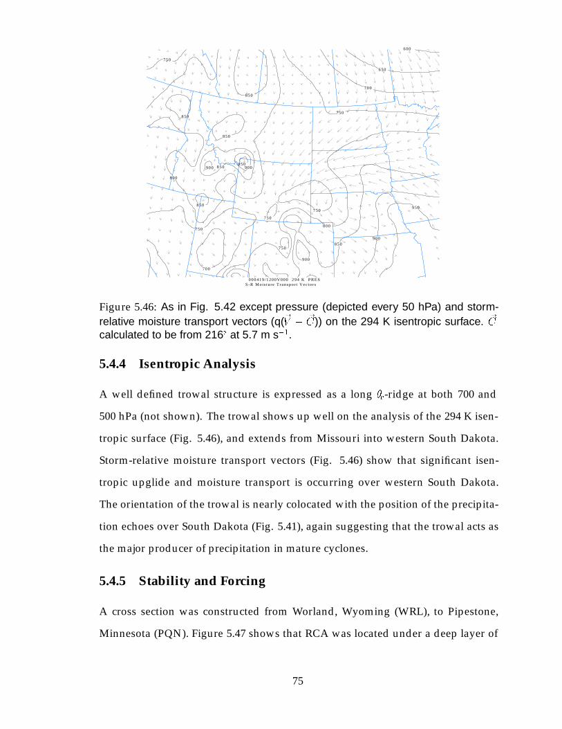
S -R Moi s tu r e T ranspo r t Vec to r s000419 /1200V000 294 K PRES

600

650

700

7 0 0

7 5 0

750

7 5 0

750

750

750

8 0 0

800

850

850

8 5 0

8 5 0

8 5 0

8 5 0

900

9009 0 0

900

950

950

Figure 5.46: As in Fig. 5.42 except pressure (depicted every 50 hPa) and storm-relative moisture transport vectors (q(~V � ~C)) on the 294 K isentropic surface. ~C

calculated to be from 216� at 5.7 m s�1.


A well defined trowal structure is expressed as a long �e-ridge at both 700 and

500 hPa (not shown). The trowal shows up well on the analysis of the 294 K isen-

tropic surface (Fig. 5.46), and extends from Missouri into western South Dakota.

Storm-relative moisture transport vectors (Fig. 5.46) show that significant isen-

tropic upglide and moisture transport is occurring over western South Dakota.

The orientation of the trowal is nearly colocated with the position of the precipita-

tion echoes over South Dakota (Fig. 5.41), again suggesting that the trowal acts as

the major producer of precipitation in mature cyclones.


A cross section was constructed from Worland, Wyoming (WRL), to Pipestone,

Minnesota (PQN). Figure 5.47 shows that RCA was located under a deep layer of

75

80

80

90

90

000419 /1200V000 RELH

2 0 0

2 5 0

3 0 0

3 5 0

4 0 0

4 5 0

5 0 0

5 5 0

6 0 0

6 5 0

7 0 0

7 5 0

8 0 0

8 5 0

9 0 0

WRL PQN

296298300302304306 308310312

314

316

318

320

322

322

324

324

326

326

328

330

332334

336338

340342

344346

348350

352

000419 /1200V000 THTE

2 0 0

2 5 0

3 0 0

3 5 0

4 0 0

4 5 0

5 0 0

5 5 0

6 0 0

6 5 0

7 0 0

7 5 0

8 0 0

8 5 0

9 0 0

WRL PQN

Figure 5.47: Vertical cross section from Worland, Wyoming (WRL), to Pipestone,Minnesota (PQN), from the 1200 UTC RUC initial field valid on 19 April 2000. Solidlines depict equivalent potential temperature (every 2 K). Values of relative humiditygreater than 80% are shaded green. RCA is located between the fifth and sixth tickmarks from the left edge.

high RH (>80%) at 1200 UTC. The contours of �e indicate that the atmosphere was

convectively stable. Mg was not calculated for this cross section because of the

heavily curved nature of the thermal wind field. The three-dimensional EPV field

(Fig. 5.48) shows that areas of WSS (<2 PVU) were located near the surface (above

RCA) and above 700 hPa, and separated by a region of fairly strong symmetric

stability (>3 PVU). As in the other cases, the three-dimensional EPV fields using

�e (Fig. 5.48) and �es (Fig. 5.49) are very similar.

The analysis of the frontogenesis and ! fields (Fig. 5.50) indicates a region of

strong frontogenesis (� 16 � 10�1 K 100 km�1 3 h�1) at 850 hPa, or just above the

surface at RCA). The strongest upward vertical motion (! � 16 �b s�1) is located

at 650 hPa (Fig. 5.50), directly above the level of strongest frontogenesis.

~Q analysis (850-400 hPa layer) at this time shows ~Qs convergence of approxi-

76

0

0

0

1

1

2

2

3

4

4

4

5

5

5

5

6

6

67 7

000419 /1200V000 EPV3 (*10**6 )

200

250

300

350

400

450

500

550

600

650

700

750

800

850

900

WRL PQN


0

0

1

1

2

2

3

3

44

4

4

5

5

5

5

6

6

67 7

8

000419 /1200V000 EPVTHES3 (*10**6 )

2 0 0

2 5 0

3 0 0

3 5 0

4 0 0

4 5 0

5 0 0

5 5 0

6 0 0

6 5 0

7 0 0

7 5 0

8 0 0

8 5 0

9 0 0

WRL PQN


77

- 18

-16

-14-12

-1 0

-8

-8

-6

-6

-4

-4

-2

-2

-2

-2

000419 /1200V000 OMEG (*10**3 )

2 0 0

2 5 0

3 0 0

3 5 0

4 0 0

4 5 0

5 0 0

5 5 0

6 0 0

6 5 0

7 0 0

7 5 0

8 0 0

8 5 0

9 0 0

WRL PQN

-20-16-12-8

-8

-4

-4

-4

0

0

0

0

0

0

0

0

4

4

4

4

4

48

8

8

8

12

12

1 2

12

16

16

1 6

20

20

20

2424

28

0 00419 /1200V000 FRNTTHTAUOBS (*10**1 )

2 0 0

2 5 0

3 0 0

3 5 0

4 0 0

4 5 0

5 0 0

5 5 0

6 0 0

6 5 0

7 0 0

7 5 0

8 0 0

8 5 0

9 0 0

WRL PQN

Figure 5.50: As in Fig. 5.47 except Petterssen surface frontogenesis (solid lines,every 4 � 10�1 K 100 km�1 3 h�1), and ! (dashed lines, every 2 �b s�1).

mately 3 � 10�14 m kg�1 s�1 (Fig. 5.51 and ~Qn convergence near zero (Fig. 5.52).

Therefore, the primary forcing mechanisms were on the synoptic scale, and were

likely related to the influence of the trowal. As in the 11 March 2000 event, the

Barnes et al. (1996) gravity wave signature is present, indicative that gravity waves

may have played a role in the enhancement of vertical motion.

5.4.6 Conclusions

The analysis generated for this event suggests that the TS that was observed at

RCA occurred primarily as a result of lower tropospheric frontogenetical forcing

in the presence of in the trowal airstream. Weak symmetric stability above the

frontogenetical layer would help enhance vertical motions. Upward vertical mo-

tion was also enhanced by strong upper tropospheric divergence in the left exit

region of a jet streak, and due to processes associated with a nearby tropopause

fold. Because of the strong easterly airstream that existed with this system, and

78

Conve rgence o f Qs (400 :850 ) ( 10e -14 )

-10

-8

-8

-6

-6

-4

-4

-4

-4

-2

-2

-2 -2

-2-2

-2

-2

-2

-2

0

0 00

0

0

0

0

0

0

0

0

0

0

000

0

0

0

0

0

00

0

0

0

0

0

0

0

00

2

2

2

2

2

2

4

4 4

4

4

4

4

6

6

6

810

12

Figure 5.51: As in Fig. 5.42 except convergence of ~Qs in the 850-400-hPa layer.Contours drawn every 2 � 10�14 m kg�1 s�1.

- 6-5

-5

-4

-4

-3

-3

-3

-2

-2

-2

-2

-2

-2

-1

-1

-1

-1 -1

-1

-1-1

-1

-1

-1

-1

-1

0

0

0

0

0

0

0

0

0

0

00

0

0

0

0

0

0

0

00

0

0

00

0

0

0

0

00

1

1

1

1

1

1

1

1

1

1

1

1

11

1

1

2

2

2

2

2

3

3

Conve rgence o f Qn (400 :850 ) ( 10e -14 )

3

3

45

Figure 5.52: As in Fig. 5.42 except convergence of ~Qn in the 850-400-hPa layer.Contours drawn every 1 � 10�14 m kg�1 s�1.

79

because of the characteristics of the terrain in western South Dakota, orographic

lift could have also played a significant role in the production of enhanced vertical

motion. However, the strong synoptic-scale influences that were associated with

this event cannot be ignored.

80

Chapter 6

Discussion and Conclusions

6.1 Discussion of Case Studies

Each of the four TS events occurred to the northwest of a surface cyclone, one of

which (19 April 2000) had occluded. While only the 19 April event was associated

with an occluded surface cyclone, all the events were associated with cyclones

that exhibited a well-defined trowal structure at some level. When radar images

and the location of trowal structures are compared, it can be stated, conclusively,

that the trowal is the major avenue of ascent and precipitation production in these

events. This is further illustrated by the analysis of moisture transport vectors

done here (Chapter 5), and by the trajectory analyses performed by Martin (1999).

The trowal is a region of frontogenesis, which is likely the single most important

forcing mechanism in the production of trowal-related precipitation and TS. In

each of the four events, the strongest upward vertical motion was located at or

above the level of the strongest frontogenesis.

None of the four cases exhibited any CSI, with two instances of upright con-

vection from the release of CI (5 December 1999, 9 December 1999) and the other

two likely from slantwise convection in the face of WSS (11 March 2000, 19 April

2000). Therefore, instability associated with TS events is likely less important than

the forcing for vertical motion.

In each event, a significant tropopause/PV anomaly was also nearby. This is

81

important for three reasons. First, tropopause folds will reduce the static stability

below them, leading to increased upward vertical motion (Hoskins et al. 1985).

Second, large amounts of cyclonic PV advection will create large amounts of abso-

lute vorticity below, thus creating conditions in which absolute vorticity advection

increases with height and enhancing QG forcing. This is well represented in the

~Qs convergence field, which was the dominant forcing mechanism in each event.

Third, as PV tries to conserve itself, the flow will become more meridional and the

cyclone will soon become negatively tilted, and the trowal structure will develop.

~Qs forcing was equal to or greater than ~Qn forcing in each of the four cases,

reinforcing what was discussed in the preceding paragraph, and concurring with

the findings of Martin (1999). The frontal-scale processes that occur in these events

occur largely due to the forcing by the large-scale flow, and in response to defor-

mation of the thermal field.

In regard to the evaluation of CI/CSI, few differences were observed between

the methods espoused by Moore and Lambert (1993) and Schultz and Schumacher

(1999). The negative EPV regions that are created by the Schultz and Schumacher

(1999) method are slightly greater, but had no bearing on the diagnosis of stability

at any of the TS locations. The Moore and Lambert (1993) yielded EPV fields with

stronger gradients. This is because the true moisture field is used in the calculation

of �e, and strong �e gradients will be reflected as strong gradients of EPV.

6.2 Conclusions

The discussion in this section will be centered on the statements that were outlined

in Section 1.1. The first contention was that there would be two regions of preferred

TS occurrence, in the trowal airstream (due to frontogenesis) in the occluded sector

of a surface cyclone, and to the northeast of a surface cyclone in advance of a warm

front. The 30-year climatology shows that this is true, at least geographically with

82

regard to the cyclone. Figure 4.7 shows that the northwest and northeast sectors are

by far the most preferred regions for the occurrence TS. The case studies illustrate

that the TS in each event occurred in the trowal airstream in the occluded sector of

the cyclone in regions of abundant frontogenetical forcing. None of the case studies

involved TS in the northeast sector, so the dynamics of these types of events cannot

be addressed.

The second contention was that CSI will be more prevalent in the northeast

sector of a cyclone and that CI will be more prevalent in the occluded sector. Again,

the first part of this contention cannot be addressed. However, of the events which

were studied, only one involved the release of CI, although another (5 December

1999) likely involved release of upright instability, even though no CI was resolved.

It is no surprise that the instability was upright in the 5 and 9 December 1999 cases

because the middle to upper tropospheric shear is cyclonic and the open-wave

cyclone still possessed a baroclinic tilt (Bluestein 1986). The flow in the 11 March

2000 case was less cyclonic, but not really anticyclonic either. Also, the system was

also an open baroclinic wave. A region of CSI is present to the southeast of STL

(Fig. 5.33), where the flow is more anticyclonic. Therefore, the shear profile was not

favorable for the occurrence of either CSI or CI. In the 19 April 2000 event, the shear

is cyclonic throughout the troposphere. However, the system was approaching an

equivalent barotropic state from the surface to 700 hPa which may have lessened

the vertical temperature profile to the point that upright instability could not occur.

So, while the second contention could not be proven, it was not disproven, either.

Because the systems that produce TS are so complex, the contention that was made

may have been oversimplified. This is because the shear and temperature profiles

will both effect the stability. A “stacked system” will possess small amounts of

vertical wind shear near the cyclone’s center, thus inhibiting the development of

symmetric instability (Bluestein 1986). At the same time, the resulting decrease in

83

lapse rates will lessen the likelihood that any upright instability will occur.

84

References

Barnes, D.A., F. Caracena, and A. Marroquin, 1996: Extracting synoptic-scale di-

agnostic information from mesoscale models: The eta model, gravity waves,

and quasigeostrophic diagnostics. Bull. Amer. Meteor. Soc., 77, 519-528.

Bennetts, D.A., and B.J. Hoskins, 1979: Conditional symmetric instability - A pos-

sible explanantion for frontal rainbands. Quart. J. Roy. Meteor. Soc., 105,

945-962.

———-, and J.C. Sharp, 1982: The relevance of conditional symmetric instability

to the prediction of mesoscale frontal rainbands. Quart. J. Roy. Meteor. Soc.,

108, 595-602.

Bluestein, H., 1986: Fronts and jet streaks: A theoretical perpspective. Mesoscale

Meteorology and Forecasting, Peter Ray, Ed., Amer. Meteor. Soc., 173-215.

Colman, B.R., 1990: Thunderstorms above frontal surfaces in environments with-

out positive CAPE. Part I: A climatology. Mon. Wea. Rev., 118, 1103-1121.

Curran, J.T., and A.D. Pearson, 1971: Proximity soundings for thunderstorms

with snow. Preprints, 7th Conference on Severe Local Storms, Kansas City, MO,

Amer. Meteor. Soc., 298-300.

Holle, R.L., J.V. Cortinas, and C.C. Robbins, 1998: Winter thunderstorms in the

United States. Preprints, 16th Conf. on Weather Analysis and Forecasting, Phoenix,

AZ, Amer. Meteor.Soc., 118-119.

Hoskins, B.J., M.E. McIntyre, and A.W. Robertson, 1985: On the use and signifi-

cance of isentropic potential vorticity maps. Quart. J. Roy. Meteor. Soc., 111,

877-946.

85

Jewett, B.F., M.K. Ramamurthy, and R.M. Rauber, 2001: The role of evaporative

processes in gravity wave genesis. Preprints, 9th Conference on Mesoscale Pro-

cesses, Ft. Lauderdale, FL, Amer. Meteor.Soc., 485-489.

Martin, J.E., 1998a: The structure and evolution of a continental winter cyclone.

Part I: Frontal structure and the occlussion process. Mon. Wea. Rev., 126,

303-328.

————., 1998b: The structure and evolution of a continental winter cyclone.

Part II: Frontal forcing of an extreme snow event. Mon. Wea. Rev., 126, 329-

348.

————, 1999: Quasigeostrophic forcing of ascent in the occluded sector of cy-

clones and the trowal airstream. Mon. Wea. Rev., 127, 70-88.

McCann, D.W., 1995: Three-dimensional computations of equivalent potential

vorticity. Wea. Forecasting, 10, 798-802.

Moore, J.T., and P.D. Blakely, 1988: The role of frontogenetical forcing and condi-

tional symmetric stability in the Midwest snowstorm of 30-31 January 1982.

Mon. Wea. Rev., 116, 2155-2171.

————, and T.E. Lambert, 1993: The use of equivalent potential vorticity to

diagnose regions of conditional symmetric instability. Wea. Forecasting, 8,

301-308.

Moore, J.T., A.C. Czarnetzki, and P.S. Market, 1998: Heavy precipitation associ-

ated with elevated thunderstorms formed in a convectively unstable layer

aloft. Meteorol. Appl., 5, 373-384.

Mote, T.L., D.W. Gamble, S.J. Underwood, and M.L. Bentley, 1997: Synoptic-scale

features common to heavy snowstorms in the southeast United States. Wea.

Forecasting, 12, 5-23.

86

Nicosia, D.J., and R.H. Grumm, 1999: Mesoscale band formation in three major

northeastern United States snowstorms. Wea. Forecasting, 14, 346-368.

O’Brien, J.J., 1970: Alternative solutions to the classical vertical velocity problem.

J. Appl. Meteor., 9, 197-203.

Sanders, F., 1986: Frontogenesis and symmetric stability in a major New England

snowstorm. Mon. Wea. Rev., 114, 1847-1862.

Schultz, D.M., and P.N. Schumacher, 1999: The use and misuse of conditional

symmetric instability. Mon. Wea. Rev., 127, 2709-2732.

Schultz, D.M., 1999: Lake-effect snowstorms in northern Utah and western New

York with and without lightning. Wea. Forecasting, 14, 1023-1031.

Schwartz, B.E., S.J. Weiss, and S.G. Benjamin, 2000: An assessment of the Rapid

Update Cycle short-range forecast fields related to convective development.

Preprints, 20th Conference on Severe Local Storms, Orlando, FL, Amer. Meteor.

Soc., 443-446.

Smith, T.L., S.G. Benjamin, B.E. Schwartz, and G. Grell, 2000: A past and future

look at the Rapid Update Cycle for the 3 May 1999 severe weather outbreak.

Preprints, 20th Conference on Severe Local Storms, Orlando, FL, Amer. Meteor.

Soc., 21-24.

Weismuller, J.L., and S.M Zubrick, 1998: Evaluation and application of condi-

tional symmetric instability, equivalent potential vorticity, and frontogenetic

forcing in an operational forecast environment. Wea. Forecasting, 13, 84-101.

87

Vita

Christopher Eric Halcomb was born on 24 February 1967 at Southeast Missouri

Hospital in Cape Girardeau, Missouri. After my parents had divorced, my mom

(Tracy) and I moved to Poplar Bluff, Missouri, where she married Richard Gant

when I was 7 years old. At the age of nine, we moved to Dexter, Missouri, from

where I graduated from high school in 1985. After spending some time at the

University of Missouri pursuing study in meteorology and respiratory therapy, I

received my Bachelor’s Degree in Geoscience from Southeast Missouri State Uni-

versity (SEMO) in 1995. Hoping to study earthquakes, I found myself involved

in the the unrewarding field of hazardous environmental clean-up in Memphis,

Tennesee. I then returned home to Cape Girardeau where I started in the BSN pro-

gram at SEMO. After a year of straight A’s, I decided that nursing was just not for

me. So I decided to go back to my true love, meteorology, and returned to Mizzou

to get my M.S.

My love for meteorology started with a shear fascination for the very active

period that was the 1970’s, but was fully realized after a surprise thunder-blizzard

paralyzed much of southeastern Missouri and southern Illinois on 25 February

1979, the day after my 12th birthday. Anywhere from 1 to 4 inches of snow was

supposed to fall, but up to 24 inches fell instead, with drifts piled up to 8 feet in

depth by winds of over 50 mph. This was the highlight of a week that featured

severe thunderstorms, heavy rain, huge temperature swings, and a solar eclipse.

After that, I was hooked!

88

case studies of midwestern thundersnow events

Documents