cascade ov

8/6/2019 Cascade Ov

http://slidepdf.com/reader/full/cascade-ov 1/24

A Multifrequency Theory of the Interest Rate

Term Structure

Laurent Calvet, Adlai Fisher, and Liuren Wu

HEC, UBC, & Baruch College

February 3, 2010

Liuren Wu (Baruch) Cascade Dynamics with Power Law Scaling February 3, 2010 1 / 24

http://find/

http://goback/

8/6/2019 Cascade Ov


Shocks to the interest rate term structure

Shocks of all frequencies come at the interest rate dynamics/term structure:

Long term: Inflation shocks tend to move the term structure inparallel; Real GDP growth shocks tend to move short rates more thanlong rates.

Intermediate term: Monetary policy shocks are often imposed at theshort end and they dissipate through the yield curve via expectations.

Short term: Supply/demand (transactions) shocks enter the yieldcurve at a particular maturity and dissipate through the yield curve viahedging and yield curve statistical arbitrage trading.

A successful term structure model must capture the effects of shocks of allfrequencies.


http://goforward/

http://find/

http://goback/

8/6/2019 Cascade Ov


The literature

Theory: Dynamic term structure models with N factors are well-developed,

with analytical tractability. Examples include the affine class (Duffie, Kan,Pan, and Singleton) and the quadratic class (Leippold and Wu).

Practice: The commonly estimated models are all low-dimensional, mostlywith three factors.

Three-factor models are successful in capturing major variations in theinterest rate level, the term structure slope, and curvature.

The remaining movements can be economically significant (in four-legtrades, Bali, Heidari, & Wu).

Three-factor models fail miserably inpredicting future interest rate movements (Duffee),capturing the cross-correlation between non-overlapping forwards (Dai& Singleton),pricing interest-rate options (Heidari & Wu, Li &Zhao).


http://goforward/

http://find/

http://goback/

8/6/2019 Cascade Ov


8/6/2019 Cascade Ov


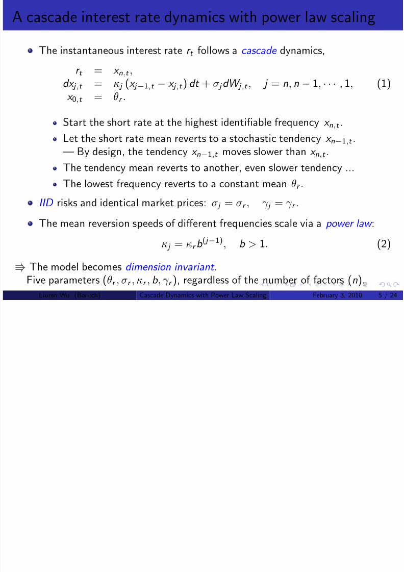
A cascade interest rate dynamics with power law scaling

The instantaneous interest rate r t follows a cascade dynamics,

r t = x n,t ,dx j ,t = κ j (x j −1,t − x j ,t ) dt + σ j dW j ,t , j = n, n − 1, · · · , 1,

x 0,t = θr .(1)

Start the short rate at the highest identifiable frequency x n,t .

Let the short rate mean reverts to a stochastic tendency x n−1,t .— By design, the tendency x n−1,t moves slower than x n,t .

The tendency mean reverts to another, even slower tendency ...

The lowest frequency reverts to a constant mean θr .

IID risks and identical market prices: σ j = σr , γ j = γ r .

The mean reversion speeds of different frequencies scale via a power law :

κ j = κr b ( j −1), b > 1. (2)

The model becomes dimension invariant .

Five parameters (θr , σr , κr , b , γ r ), regardless of the number of factors (n).Liuren Wu (Baruch) Cascade Dynamics with Power Law Scaling February 3, 2010 5 / 24

http://goforward/

http://find/

http://goback/

8/6/2019 Cascade Ov


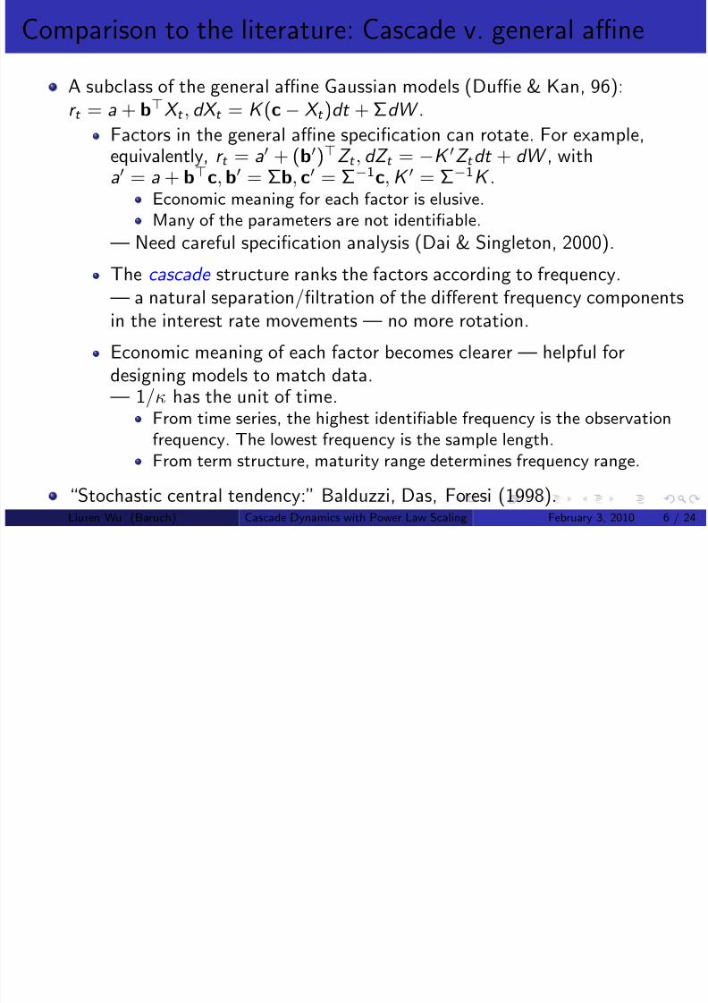
Comparison to the literature: Cascade v. general affine

A subclass of the general affine Gaussian models (Duffie & Kan, 96):r t = a + bX t , dX t = K (c − X t )dt + ΣdW .

Factors in the general affine specification can rotate. For example,equivalently, r t = a + (b)Z t , dZ t = −K Z t dt + dW , witha = a + bc, b = Σb, c = Σ−1c, K = Σ−1K .

Economic meaning for each factor is elusive.Many of the parameters are not identifiable.

— Need careful specification analysis (Dai & Singleton, 2000).The cascade structure ranks the factors according to frequency.— a natural separation/filtration of the different frequency componentsin the interest rate movements — no more rotation.

Economic meaning of each factor becomes clearer — helpful for

designing models to match data.— 1/κ has the unit of time.

From time series, the highest identifiable frequency is the observationfrequency. The lowest frequency is the sample length.From term structure, maturity range determines frequency range.

“Stochastic central tendency:” Balduzzi, Das, Foresi (1998).Liuren Wu (Baruch) Cascade Dynamics with Power Law Scaling February 3, 2010 6 / 24

http://goforward/

http://find/

http://goback/

8/6/2019 Cascade Ov


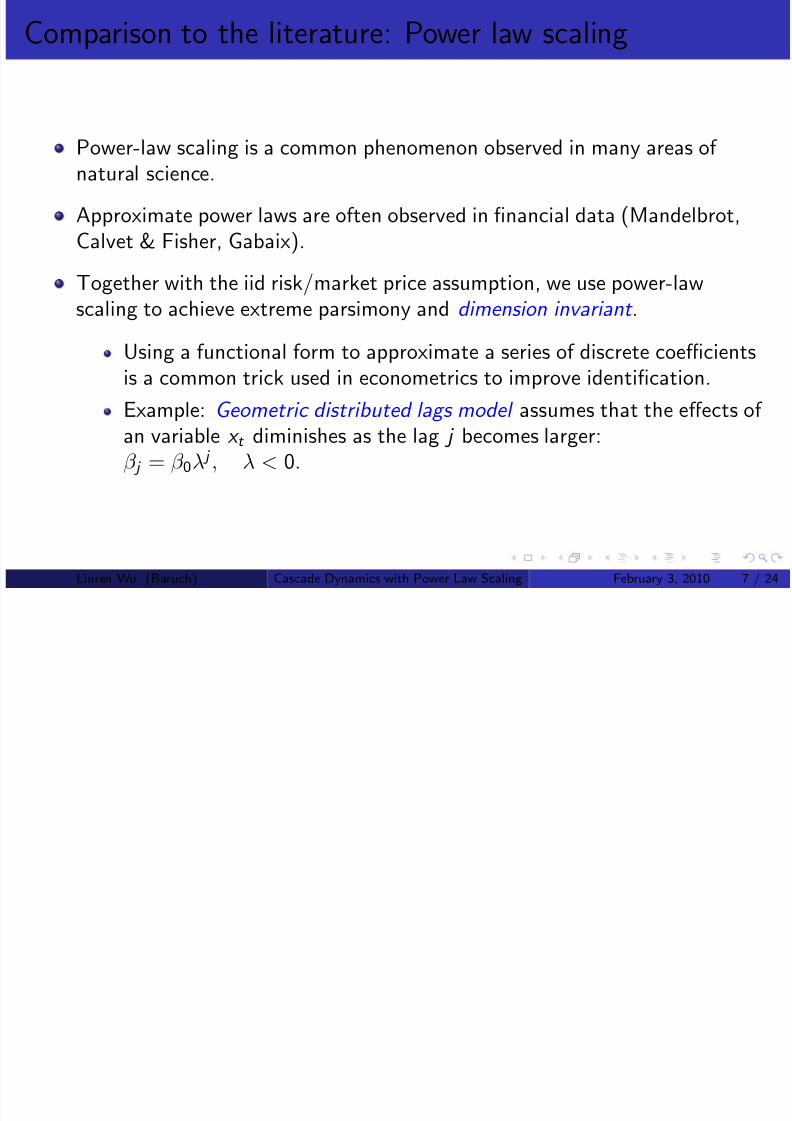
Comparison to the literature: Power law scaling

Power-law scaling is a common phenomenon observed in many areas of natural science.

Approximate power laws are often observed in financial data (Mandelbrot,Calvet & Fisher, Gabaix).

Together with the iid risk/market price assumption, we use power-lawscaling to achieve extreme parsimony and dimension invariant .

Using a functional form to approximate a series of discrete coefficientsis a common trick used in econometrics to improve identification.

Example: Geometric distributed lags model assumes that the effects of an variable x t diminishes as the lag j becomes larger:β j = β 0λ j , λ < 0.


http://goforward/

http://find/

http://goback/

8/6/2019 Cascade Ov


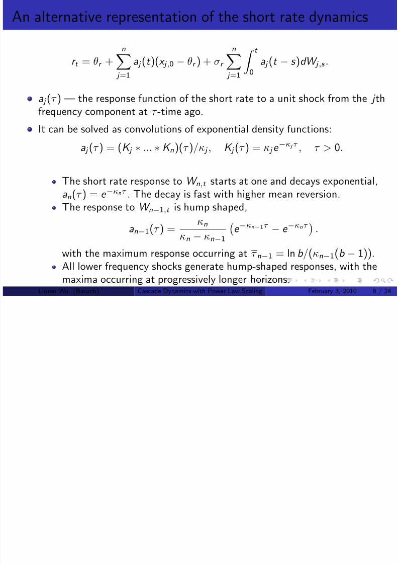
An alternative representation of the short rate dynamics

r t = θr +

n

j =1

a j (t )(x j ,0 − θr ) + σr

n

j =1

t

0

a j (t − s )dW j ,s .

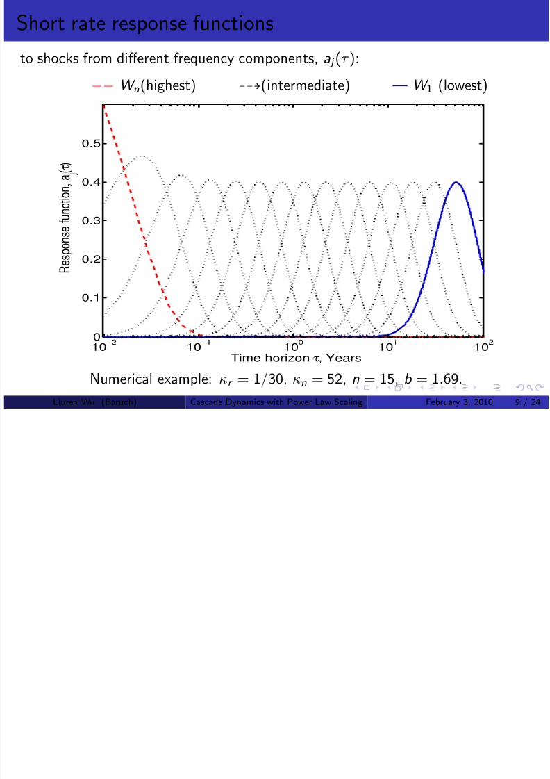
a j (τ ) — the response function of the short rate to a unit shock from the j thfrequency component at τ -time ago.

It can be solved as convolutions of exponential density functions:

a j (τ ) = (K j ∗ ... ∗ K n)(τ )/κ j , K j (τ ) = κ j e −κ j τ , τ > 0.

The short rate response to W n,t starts at one and decays exponential,an(τ ) = e −κnτ . The decay is fast with higher mean reversion.

The response to W n−1,t is hump shaped,

an−1(τ ) =κn

κn − κn−1

e −κn−1τ − e −κnτ

.

with the maximum response occurring at τ n−1 = ln b /(κn−1(b − 1)).All lower frequency shocks generate hump-shaped responses, with the

maxima occurring at progressively longer horizons.Liuren Wu (Baruch) Cascade Dynamics with Power Law Scaling February 3, 2010 8 / 24

http://goforward/

http://find/

http://goback/

8/6/2019 Cascade Ov


Short rate response functions

to shocks from different frequency components, a j (τ ):

−− W n(highest) (intermediate) — W 1 (lowest)

10−2

10−1

100

101

102

0

0.1

0.2

0.3

0.4

0.5

Time horizon τ, Years

R e s p o n s e f u n c t i o n ,

a j ( τ

)

Numerical example: κr = 1/30, κn = 52, n = 15, b = 1.69.Liuren Wu (Baruch) Cascade Dynamics with Power Law Scaling February 3, 2010 9 / 24

http://goforward/

http://find/

http://goback/

8/6/2019 Cascade Ov


Unconditional variance and the limit behavior

The unconditional variance of the short rate has an upper bound,

Var (r t ) = σ2r

n j =1

∞

0

a2 j (s )ds ≤ σ2

r

n j =1

∞

0

a j (s )ds = σ2r

n j =1

1

κ j

< ∞.

as long as κ j > 0.

Under power law scaling, the upper bound becomes,

Var (r t ) ≤ σ2r

n j =1

1

κ j

=σ2r

κr

1 − b −n

1 − b −1.

The short rate has finite variance regardless of how many factors we add tothe dynamics.

The limit exists as n → ∞.

The unconditional variance contribution of higher frequency componentsbecomes progressively smaller.


http://goforward/

http://find/

http://goback/

8/6/2019 Cascade Ov


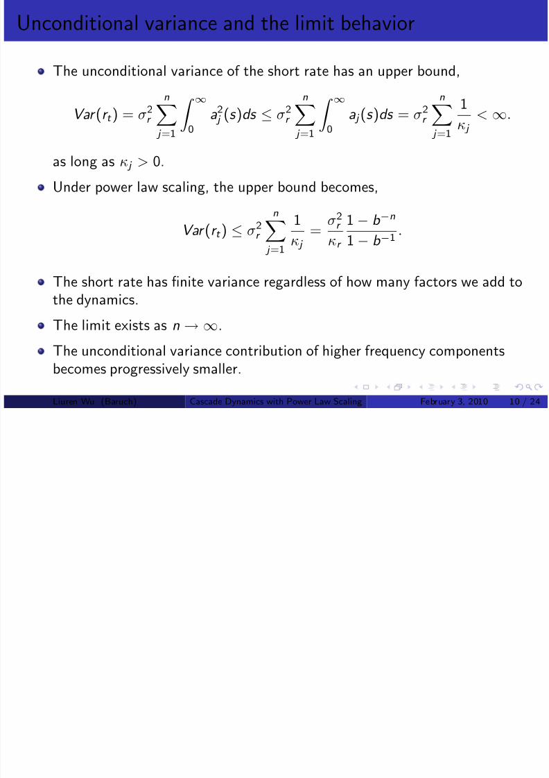
Bond pricing

The values of zero-coupon bonds are exponential-affine in X t = {x j ,t }n j =1,

P (X t , τ ) = EPt

exp

−

T

t

r s ds

E

−

T

t

γ s · dX s

= e −b (τ )X t −c (τ ),

The instantaneous forward rate is affine in the state vector,

f (X t , τ ) = a (τ )X t + e (τ ) ,

The short rate response function a(τ ) across different time lags alsodetermines the contemporaneous response of the forward rate curve.

10−2

10−1

100

101

102

0

0.1

0.2

0.3

0.4

0.5

Time horizon τ, Years

R e s p o n s e f u n c t i o n

, a j ( τ

)

a(τ ) — fixed basis functionsX t — time-varying weights.


http://goforward/

http://find/

http://goback/

8/6/2019 Cascade Ov


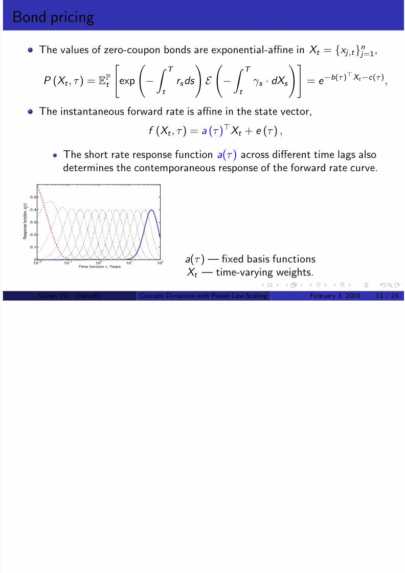
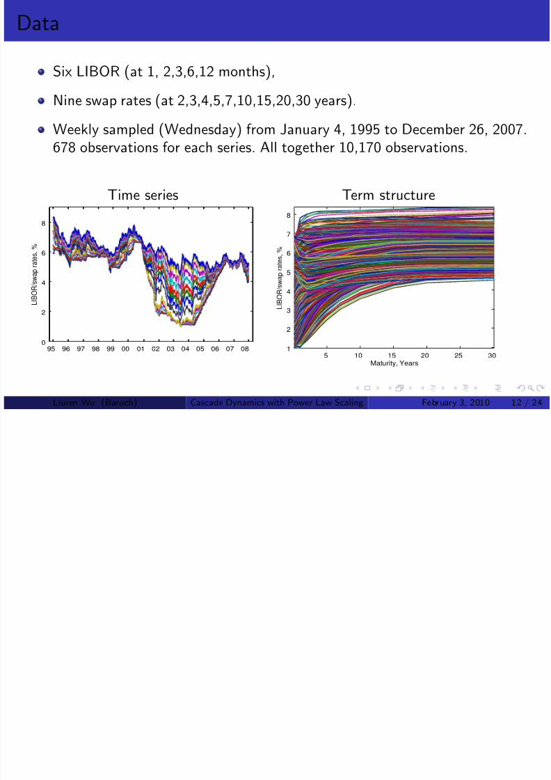
Data

Six LIBOR (at 1, 2,3,6,12 months),

Nine swap rates (at 2,3,4,5,7,10,15,20,30 years).

Weekly sampled (Wednesday) from January 4, 1995 to December 26, 2007.678 observations for each series. All together 10,170 observations.

Time series Term structure

95 96 97 98 99 00 01 02 03 04 05 06 07 08

0

2

4

6

8

L I B O R

/ s w a p r a t e s ,

%

5 10 15 20 25 301

2

3

4

5

6

7

8

Maturity, Years

L I B O R / s w a p r a t e s ,

%


http://goforward/

http://find/

http://goback/

8/6/2019 Cascade Ov


8/6/2019 Cascade Ov


Dimensionality

Normally, this is the first thing one decides on before one can pin down the

parameter space.

Under our model, the parameter space is invariant to the dimensionalitydecision. We worry about the dimensionality the last.

Since we have 15 interest rate series, we estimate 15 models with

n = 1, 2, 3, · · · 15.

The estimations of these models are equally easy and fast.

The extensive estimation exercise serves at least two purposes:

Determine how many frequency components the data ask for — Thisnormally depends on the data one uses. More maturities wouldnaturally ask for more frequency components.Analyze how high-dimensional models differ from low-dimensionalmodels in performance.


http://goforward/

http://find/

http://goback/

8/6/2019 Cascade Ov


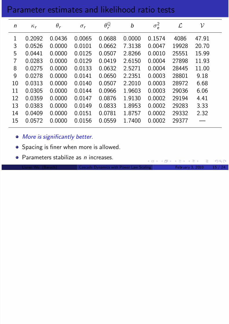
Parameter estimates and likelihood ratio tests

n κr θr σr θQr b σ2e L V

1 0.2092 0.0436 0.0065 0.0688 0.0000 0.1574 4086 47.913 0.0526 0.0000 0.0101 0.0662 7.3138 0.0047 19928 20.705 0.0441 0.0000 0.0125 0.0507 2.8266 0.0010 25551 15.997 0.0283 0.0000 0.0129 0.0419 2.6150 0.0004 27898 11.938 0.0275 0.0000 0.0133 0.0632 2.5271 0.0004 28445 11.009 0.0278 0.0000 0.0141 0.0650 2.2351 0.0003 28801 9.18

10 0.0313 0.0000 0.0140 0.0507 2.2010 0.0003 28972 6.6811 0.0305 0.0000 0.0144 0.0966 1.9603 0.0003 29036 6.0612 0.0359 0.0000 0.0147 0.0876 1.9130 0.0002 29194 4.4113 0.0383 0.0000 0.0149 0.0833 1.8953 0.0002 29283 3.3314 0.0409 0.0000 0.0151 0.0781 1.8757 0.0002 29332 2.32

15 0.0572 0.0000 0.0156 0.0559 1.7400 0.0002 29377 —

More is significantly better.

Spacing is finer when more is allowed.

Parameters stabilize as n increases.Liuren Wu (Baruch) Cascade Dynamics with Power Law Scaling February 3, 2010 15 / 24

http://goforward/

http://find/

http://goback/

8/6/2019 Cascade Ov


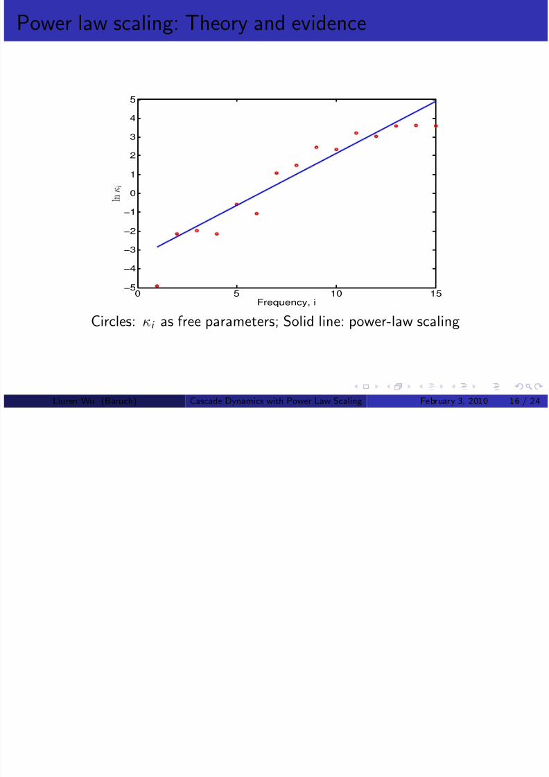
Power law scaling: Theory and evidence

0 5 10 15−5

−4

−3

−2

−1

0

1

2

3

4

5

Frequency, i

l n

κ i

Circles: κi as free parameters; Solid line: power-law scaling


I l fi i f P i i i i

http://goforward/

http://find/

http://goback/

8/6/2019 Cascade Ov


In-sample fitting performance: Pricing error statistics

Model A. Three-factor model B. 15-factor model

Maturity Mean Rmse Auto Max VR Mean Rmse Auto Max VR

1 m -0.68 7.47 0.86 43.93 99.83 0.02 0.62 0.36 5.40 100.002 m 0.63 3.82 0.69 37.42 99.96 0.01 1.76 0.52 16.31 99.993 m 1.61 5.03 0.85 42.54 99.93 -0.11 1.79 0.60 18.96 99.996 m 0.39 6.78 0.93 24.05 99.86 0.04 1.06 0.59 8.78 100.009 m -1.74 6.88 0.89 32.06 99.86 0.38 0.92 0.69 4.31 100.00

1 y -3.06 6.74 0.79 33.00 99.88 -0.49 1.21 0.06 4.71 100.002 y 2.11 6.17 0.81 24.38 99.86 0.28 1.09 -0.02 4.52 100.003 y 1.97 6.90 0.88 34.12 99.78 -0.19 0.75 0.36 3.88 100.004 y 0.87 6.32 0.90 33.48 99.76 -0.04 0.81 0.16 8.08 100.005 y -0.21 5.85 0.90 27.63 99.76 0.07 0.73 0.20 4.60 100.00

7 y -1.89 5.55 0.92 17.32 99.77 0.08 0.70 0.35 6.86 100.0010 y -2.35 5.17 0.89 18.65 99.78 -0.12 0.95 0.23 9.00 99.9915 y 0.88 3.87 0.86 13.14 99.82 0.00 0.72 0.29 4.68 99.9920 y 1.91 5.35 0.90 17.64 99.66 0.08 0.79 0.33 6.90 99.9930 y -0.76 9.67 0.95 31.88 98.68 -0.09 0.71 0.23 4.82 99.99

Average -0.02 6.11 0.87 28.75 99.75 -0.00 0.98 0.33 7.45 99.99Liuren Wu (Baruch) Cascade Dynamics with Power Law Scaling February 3, 2010 17 / 24

A li i Yi ld i i

http://goback/

http://goforward/

http://find/

http://goback/

8/6/2019 Cascade Ov


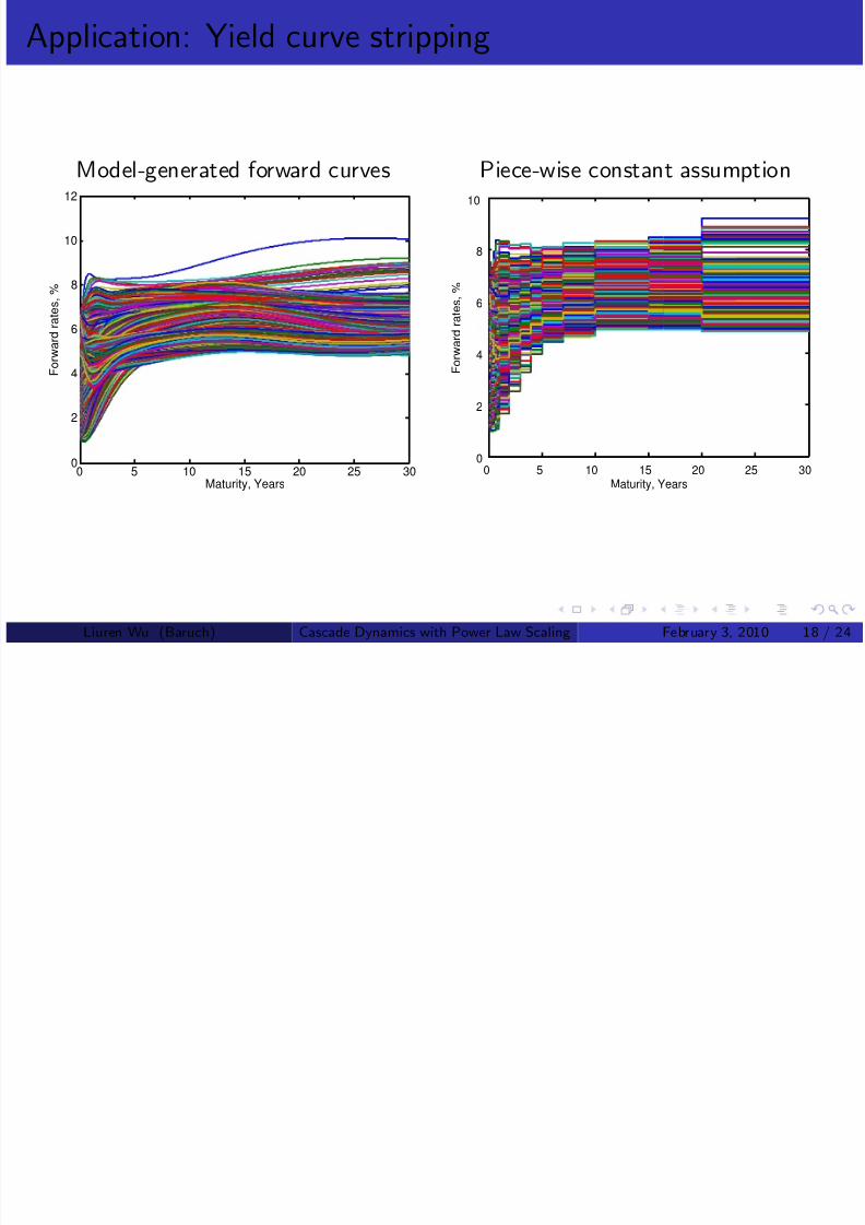
Application: Yield curve stripping

Model-generated forward curves Piece-wise constant assumption

0 5 10 15 20 25 300

2

4

6

8

10

12

Maturity, Years

F o r w a r d r a t e s

, %

0 5 10 15 20 25 300

2

4

6

8

10

Maturity, Years

F o r w a r d r a t e s ,

%


A li i Yi ld i i

http://goforward/

http://find/

http://goback/

8/6/2019 Cascade Ov


Application: Yield curve stripping

No parameter estimation is needed for practical application of stripping.

Use κi or (κr , b ) to match maturities on the curve.

Use θr and γ r to match the short and long-end of the curve.

Fix σr to historical values (effects are small on the term structure).

Fixing the parameters amounts to fixing the basis functions.

Choose the states/weights X t to match the curve.

Similar to Nelson-Siegel, with two advantages:

Dynamic consistency.

No longer limit to a three-factor structure — Near-perfect fitting is amust for stripping swap rate curves.


C l ti b t kl h

http://goforward/

http://find/

http://goback/

8/6/2019 Cascade Ov


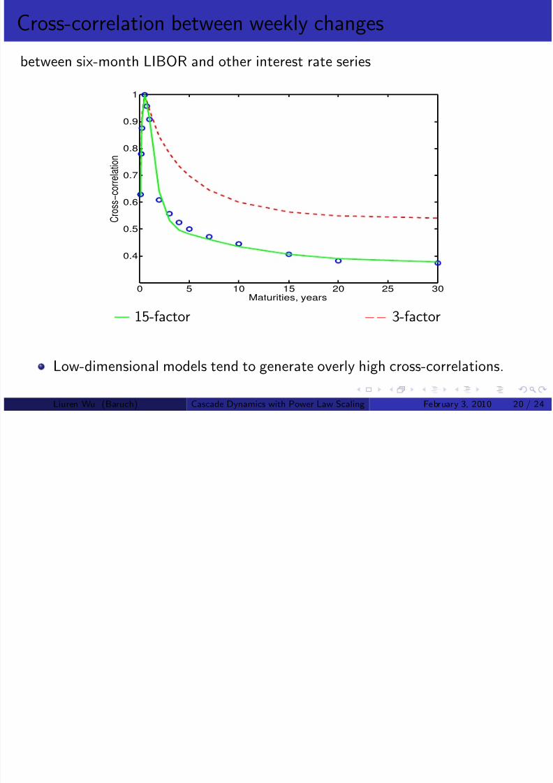
Cross-correlation between weekly changes

between six-month LIBOR and other interest rate series

0 5 10 15 20 25 30

0.4

0.5

0.6

0.7

0.8

0.9

1

Maturities, years

C r o s s −

c o r r e l a t i o n

— 15-factor −− 3-factor

Low-dimensional models tend to generate overly high cross-correlations.


I l f ti f

http://goforward/

http://find/

http://goback/

8/6/2019 Cascade Ov


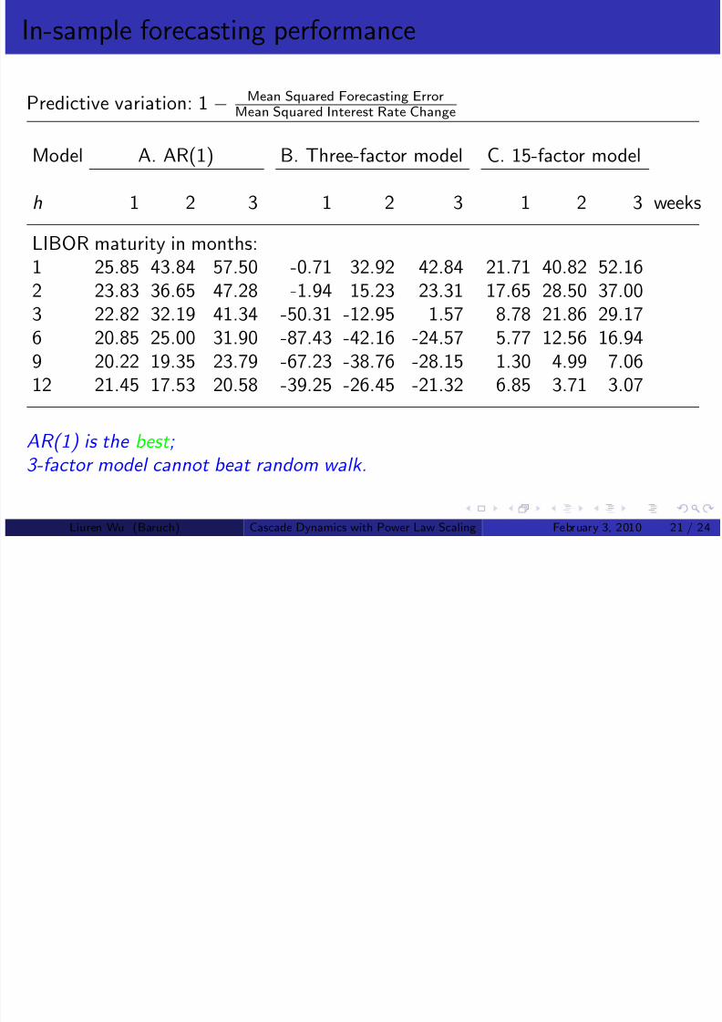
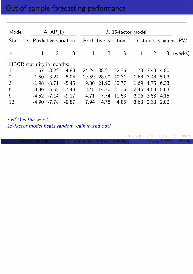
In-sample forecasting performance

Predictive variation: 1 − Mean Squared Forecasting ErrorMean Squared Interest Rate Change

Model A. AR(1) B. Three-factor model C. 15-factor model

h 1 2 3 1 2 3 1 2 3 weeks

LIBOR maturity in months:1 25.85 43.84 57.50 -0.71 32.92 42.84 21.71 40.82 52.162 23.83 36.65 47.28 -1.94 15.23 23.31 17.65 28.50 37.003 22.82 32.19 41.34 -50.31 -12.95 1.57 8.78 21.86 29.176 20.85 25.00 31.90 -87.43 -42.16 -24.57 5.77 12.56 16.949 20.22 19.35 23.79 -67.23 -38.76 -28.15 1.30 4.99 7.06

12 21.45 17.53 20.58 -39.25 -26.45 -21.32 6.85 3.71 3.07

AR(1) is the best ;3-factor model cannot beat random walk.


http://goforward/

http://find/

http://goback/

8/6/2019 Cascade Ov


Where does the forecasting strength come from?

8/6/2019 Cascade Ov


Where does the forecasting strength come from?

AR(1) regression neither uses the term structure information nor is itparsimonious.

To exploit the term structure information, need a VAR(1) structure.One AR(1) on each series, 15 × 2 = 30 parameters already!Forget about a general VAR(1).

Our model can be regarded as a constrained VAR(1):

Exploits information on the term structure.Parsimony generates out-of-sample stability for all our models.

... as simple as possible, but not simpler .

Low-dimensional models cannot even fit — The forecast is almostsurely wrong over short horizons.

If the fitting error is 6 bps, the forecasting error over the next secondwill also be 6bps — no hope of beating random walk.

Our high-dimensional model is:

simple and stable: Similar in and out of sample performance.flexible and fits perfectly: The forecast starts at the right place.


Concluding remarks

http://goforward/

http://find/

http://goback/

8/6/2019 Cascade Ov


Concluding remarks

Within the DTSM framework, we make several key assumptions:

A cascade factor structure : Eliminate factor rotation. Pin down themeaning of each factor. Provide a natural separation/filtration of different frequency components.

IID risk and risk premium: Two parameters to control the risk and riskpremium of all risks.

Power law scaling : Two parameters to control the mean reversionspeeds of all frequencies.

The result is a class of dimension-invariant models:The number of parameters is invariant to the number of factors.

No more curse of dimensionality: high-dimensional models are just aseasy to be estimated as low-dimensional models.

Evidence: High-dimensional models do provide superior performance inseveral fronts.


http://goforward/

http://find/

http://goback/

cascade ov

Documents