cas-34, no. 1, january eigenfilters: a new approach to least-squares fir filter design and...

IEEE TRANSACTIONS ON CIRCUITS AND SYSTEMS, VOL. CAS-34, NO. 1, JANUARY 1987 11

Eigenfilters: A New Approach to Least-Squares FIR Filter Design and Applications

Including Nyquist Filters P. P. VAIDYANATHAN, MEMBER, IEEE, AND TRUONG Q. NGUYEN, STUDENT MEMBER, IEEE

Abstract-A new method of designing linear-phase FIR filters is proposed by minimizing a quadratic measure of the error in the passband and stopband. The method is based on the computation of an eigenvector of an appropriate real, symmetric, and positive-definite matrix. The proposed design procedure is general enough to incorporate both time- and frequency-domain constraints. For example, Nyquist filters can be easily designed using this approach. The design time for the new method is comparable to that of Remez exchange techniques. The passband and stopband errors in the frequency domain can be made eqniripple by an iterative process, which involves feeding back the approximation error at each iteration. Several numerical design exahples and comparisons to existing methods are presented, which demonstrate the usefulness of the present approach.

I. INTRODUCTION

I T IS WELL KNOWN that most linear-phase finite impulse response filter (FIR) design problems can be

satisfactorily handled by using the McClellan-Parks (MP) algorithm [l] for weighted equiripple filters. These filters have the advantage of providing the designer with the most

optimal design in the sense of smallest filter length for a given set of specifications. In contrast, a number of authors have also considered the least-squares approach for FIR filter design [2]-[6]. As outlined in [5], [6], and [31], there are some advantages under certain situations where these methods have to be preferred over the Remez exchange techniques.’ Most least-squares techniques advanced so far are based on solving a set of linear simultaneous equations by matrix inversion.

Consider a typical low-pass design problem: we wish to approximate a “desired response” D(w) with a type-l linear-phase FIR filter transfer function H(z)

N-l

H(z) = 1 h,z-“. n=O

(A type-l filter has h, = h,-, --n and, moreover, the order

Manuscript received December 6, 1985; revised May 22, 1986. This work was supported in part by the National Science Foundation under Grant ECS 84-04245, and in part by Caltech’s programs in Advanced Technology grant, sponsored by Aerojet General, General Motors, GTE, and TRW.

The authors are with the Department of Electrical Engineering, Cali- fornia Institute of Technology, Pasadena, CA 91125.

IEEE Log Number 8611114. “‘Remez exchange algorithm” and the “MP approach” are used syn-

onymously in this paper.

N - 1 is even [7].) The desired response is

whereas the amplitude response of H(z) is [7] N-l

H,(ej”)= c h,e-j(n-M)u= f b,cosnw (3) n=O

where M = (N - 1)/2 and n=O

n#O n=O’ (4

The least-squares (LS) approach [2] to this problem is to formulate an objective function

(5) where R is the region 0 < o < 7~, but excluding the transition band. The parameters b,, are found by minimizing E,,. The actual computation of b, can be performed [2] by solving simultaneously a set of linear equations (or by matrix inversion)

b=A-‘C (6) where b = (b,b, . . * bM)‘; c and A are quantities depending upon wp and 0s. By incorporating a weighting function into the integrand of (5), one can attain a tradeoff between passband and stopband accuracies.

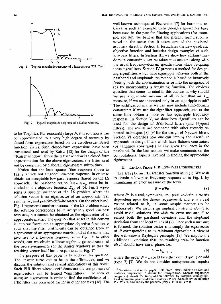
Several interesting design examples can be found in [2]. Fig. 1 shows a typical magnitude response ]Ha(ej”)] of such a least-squares FIR filter. A particular special case of the above approach gives rise to the prolate-spheroidal wave sequence as the solution [2]. This corresponds to minimizing

ELS=/n[D(cd)-HO(ejw)]2$ w s

under a suitable constraint (such as 1.h: = 1). The resulting amplitude response’is typically shown in Fig. 2. The prolate-spheroidal solution vector h = [ha, h,, * * . , h N- J’ (and, hence, 6) can be found as the eigenvector of a real, symmetric, and positive-definite matrix [2] (which happens

0098-4094/87/0100-0011$01.00 01987 IEEE

12 IEEE TRANSACTIONS ON CIRCUITS AND SYSTEMS, VOL. CM-34, NO. 1, JANUARY 1987

Fig. 1. Typical magnitude response of a least-squares FIR filter.

*

Fig. 2. Typical magnitude response of a Kaiser window

to be Toeplitz). For reasonably large N, this solution h can be approximated to a very high degree of accuracy by closed-form expressions based on the zeroth-order Bessel function I,(X). Such closed-form expressions have been introduced and used by Kaiser [IS] for the design of the “Kaiser window.” Since the Kaiser window is a closed-form approximation for the above eigenvectors, the latter need not be computed by elaborate eigensystem subroutines.

Notice that the least-squares filter response shown in Fig. 2 is itself not a “good” low-pass response; in order to obtain an acceptable low-pass response (based on the LS approach), the passband region 0 Q w G op must be in- cluded in the objective function E,, of (5). Fig. 2 represents a specific instance of the LS problem where the solution vector is an eigenvector of an appropriate real, symmetric, and positive-definite matrix. On the other hand, Fig. 1 represents another instance of the LS problem where the solution corresponds to an acceptably good low-pass response, but cannot be obtained as the eigenvector of an appropriate matrix. The question that arises in this context

’ is, can we formulate an appropriate objective function E such that the filter coefficients can be obtained from an eigenvector of an appropriate matrix, and at the same time

.give rise to a lqw-pass response as in Fig. l? In other words, can we obtain a linear-algebraic generalization of the prolate-sequences (or the Kaiser window) so that the resulting vector itself has a response as in Fig. l?

The purpose of this paper is to address this question. The answer turns out to be in the affirmative, and we discuss the solution and several applications of this result. Such FIR filters whose coefficients are the components of eigenvectors will be termed “eigenfilters.” The idea of using an eigenvector in order to find the coefficients of a FIR filter has been used earlier in other contexts [16]. The

well-known technique of Pisarenko I[171 for harmonic re- trieval is such an example. Even though eigenvectors have been used in the past for filtering applications (for example, see [6]), we believe that the present formulation is novel in the sense that it takes care of the passband accuracy directly. Section II formulates the new quadratic objective function and includes design examples of such low-pass filters. In Section III, we show how certain time- domain constraints can be taken into account along with the usual frequency-domain specifications while designing these eigenfilters. Section IV presents, a method for designing eigenfilters which have equiripple behavior both in the passband and stopband; the method is based on iteratively feeding back the approximation error into the integrand of (5) by incorporating a weighting function. The obvious question that comes to mind in this context is, why should we use a quadratic measure at all, rather than an L, measure, if we are interested only in an equiripple result? The justification is that we can now include time-domain constraints if we use the eigenfilter approach, and at the same time obtain a more or less equiripple frequency response. In Section V, we show how eigenfilters can be used for the design of Mth-band filters (and Nyquist filters). The results are compared with other recently reported techniques [8], [9] for the design of Nyquist filters. Section VI describes how one can employ the eigenfilter approach to design filters which have flatness constraints (or tangency constraints) at any given frequency in the passband. In the last section, we make comments on the computational aspects involved in finding the appropriate eigenvector.

II. LINEAR PHASE FIR LOW-PASS EIGENFILTERS

Let H(z) be an FIR transfer function as in (1). We wish to obtain a low-pass frequency resp’onse as in Fig. 1, by minimizing an error measure of the form

E = v’Pv (8) where P* is a real, symmetric, and positive-definite matrix depending upon the design requirement, and v is a real vector related to h, in some simple manner (to be elaborated). We assume an implicit constraint v’v =1 to avoid trivial solutions. We wish the error measure E to reflect both the passband deviation and the stopband deviation from the ideal values of (2). Once such a measure is formed, the solution vector v is simply the eigenvector of P corresponding to its minimum eigenvalue in view of the well-known Rayleigh’s principle [19]. We impose the additional condition that the resulting transfer function H(z) should have linear phase, i.e.,

h, = hN-l-n (9) where the order N - 1 could be either even (type 1) or odd (me 2) [71. W e d o not consider antisymmetric impulse

2Notations used in the paper: Bold-faced ktters indicate vectors and matrices. Superscript t stands for transposition, whereas superscript dagger (t) stands f?r transposition ,followed by complex conjugation. Real symmetric posthve-definite matrices P are mdlcated by the notation P = P > 0, and satisfy the property y’Py > 0 for all y Z 0.

VAIDYANATHAN AND NGUYEN: FIR FILTER DESIGN AND APPLICATIONS 13

response sequences in this section because they cannot be used in low-pass designs 171.

With H(z) satisfying (9) its frequency response takes the form

ff( e.iu) = e-AN-W*~~O( eja) (10) where H,(ej”) is real-valued, given by [7]

I

; b,,cosno, N-l even

H,(ej”) = T-O1

nZCobncos( n + $4

(10 N-l odd

The quantity M in (11) is defined as M = (N - 1)/2 for even N - 1, and it4 = N/2 for odd N - 1. Defining

b= [bo b,-.*b,-, kwli,

i

N-l even

[b, b, . ..b.-, b,,,-$, N-l odd (124

measure for the passband can be taken as

Ep=~~~pe;(w)do=;~~b’(l-c)(l-c)ibdw (18)

which can be written in the form

Ep = biPpb 0%

where Pp is given by

and is a real, symmetric, positive-definite matrix (unless wP = 0). Thus, the total measure to be minimized is

E = b’Pb (21)

where P=(l-a)Pp+aPs: (22)

The quantity (Y, which is in the range 0 < (Y 6 1, controls

and

i

P cos w cos2w * : -c0sM&$, N-l even c(o) =

[

Cd 3w N-l odd

ow cos -

2 cos - . .

2

ive can write (11) as the relative accuracies of approximation in the pass and H,(ej”) = b%(o). (13) stopbands. Notice that the elements of P are given by

For notational simplicity, c(w) will often be denoted as c. For even N - 1, the quantities b, are as in (4). For odd l-cosno)(l-cosmw)dw N - 1, b,, = 2h,-,-,.

p(n,m)=tiJYp( ?? 0

With the “desired response” as in (2), the “stopband 77 error” can now be defined as

+E J( cosnwcosrnw)do, Nodd (23a) 7T %

Es=L~~[D(~)-Ho(e~~)]2dti=~~Tbrccibd~=brPsb +Jr 0.9 s

04) where P, is given by

and is a real, symmetric, and positive definite matrix (unless ws = 7r, which is a case of no interest).

If the passband error measure Ep is also defined according to the integral of (5), the total error measure cannot be written in the form (8). Accordingly, let us define fP differently. First, notice that the zero-frequency response is given by

H,( ej”) = l’b 06) where the vector 1 is defined as

1 = [ll f *. 11’. (17) The quantity e,,(w) = (1 - c)‘b, therefore, represents the deviation of the response H,(ej”) from the zero-frequency response. 3 Accordingly, a positive-valued (quadratic) error

3The only motivation for taking zero-frequency as a reference for passband error formulation is that it brings the vector b into the reference, and this enables us to write Ep as a quadratic in b. This in turn leads to the eigenformulation.

.(I-cos(rn+fjo)do

+i[[cos(n+f)w][cos(m+f)u]do,

N even. (23b)

In summary, we have been able to formulate the linear- phase low-pass FIR design problem in the form of an eigenproblem. Given the band edges wP and os, and the parameter (Y, the matrix P can be computed. It is easy to obtain closed-form expressions for the integrals in (23), and, hence, the elements P(n, m) are easily computed once CY, wP and ws are known. It then remains only to compute the eigenvector of a real, symmetric, and positive-definite matrix corresponding to the smallest eigenvalue. The resulting filter is guaranteed to have linear phase because the vector b rather than the vector h is directly involved in the optimization problem. The eigenvector b can be used to obtain the filter coefficients h, in (1). We now proceed with design examples to demonstrate the procedures.

IEEE TRANSACTIONS ON CIRCUITS AND SYSTEMS, VOL. CA,%34, NO. 1, JANUARY 1987

I.500

NORNRLIZEO FREOUENCY

Fig. 3. (Fx 1) Magnitude response plot of Kaiser window using eigenfilter and Z(p) approximation.

0.

-80.000 0. 0.100 0.200 0.300 0.400

NORflALIZEO FREEUENCY

(4

0.900 1 I 0. 0.030 0.060 0.090 0.120 0.150

NORRALIZEO FREQUENCY

(b) Fig. 4. (Ex. 2) (a) Ma nitude response plot of FIR eigenfilter.

(b) Passban % detads for the FIR eigenfilter.

Example 1: Let w, = 0.05~ and let (Y =l in (22). Then wp does not enter into the optimization problem. With N - 1 = 30, the eigenvector b corresponding to the minimum eigenvalue of P was computed. The resulting frequency response H,,(e@) is shown in Fig.. 3 in solid lines. The broken line represents the transform of the

H,(elW) wp+w* = n

Fig. 5. Typical amplitude response of a half-band FIR filter.

Kaiser window for a window length of 31, and an appropriate value of the window parameter [7] given by p = 2.0. This example’ is only a .demonstration that the Kaiser window is an excellent closed-form approximation for certain eigenfilters (the prolate spheroidal sequences).

Example 2: A low-pass filter with N - 1 = 28, wp = 0.3n, ws = 0.41r, and (Y = 0.1 was designed using the above approach. The resulting frequency response is shown in Fig. 4, which also includes the plot for the case of (Y = 0.5. The effect of (Y is clearly seen from the figure.

Comments on the Choice of (Y: It is ‘clear from (22) that a larger value of (Y leads to better stopband attenuation at the cost of increased passband ripple. Given the set of specifications wp, ws, p assband tolerance 6, and stopband tolerance 6,, it is necessary to estimate N - 1 and (Y in order to design the eigenfilter. An approximate estimate for N - 1 can be obtained based on the relations in [20]. Even though the estimates in [20] hold only for equiripple designs, the required order for an eigenfilter is only slightly larger. The choice of a governs the ratio 8,/a,. At this

time, we do not have a procedure for estimating (Y, starting from a desired 8,/S, ratio. Further study of the behavior of eigenfilters is necessary in order to fill this gap.

The following example demonstrates the design of a half-band filter [8], [ll] based on the eigenfilter approach. For this example, the quantity (Y does not come into the picture at all, in view of the indirect procedure described below.

Example 3: A linear-phase FIR half-band filter is a type-l low-pass filter having an amplitude response H,(e@) that is symmetric with respect to r/2 as shown in Fig. 5. Note that wp + ws = rr, and 6, = 6, for such filters. It can be shown that for such filters h, satisfies

N-l h,=O for n - - =: even # 0.

2 (24)

A direct design of such filters based on any design meth- odology (such as the McClellan-Park:s program, or eigenfilter methods) invariably leads to a filter which does not satisfy (24) exactly, due to the computational inaccuracies. In addition, since about half of the impulse response coefficients are known anyway, it is only judicious to eliminate the known variables from the design problem so as to reduce computational time. This can be accomplished by designing H(z) by a two-stage process. The first step is


Go(e% \‘“. Fig. 6. Amplitude response of C(r).

1.000

0.600

0.400

0.200

0. * 0. 0.100 0.200 0.300 0.ri00 0.500

NORflRLIZEO FREQUENCY

(4

1.000

Y 2 L

0.382

z E

0.376

0.370 2 0. 0.013 0.085 0.128 0.170 0.213

NORliALIZEO FREEUENCY

(b)

Fig. 7. (Ek. 3) (a) Response of the half-band ei enfilter. (b) Passband details for the half-band eigenfl ter. .k

the design of a one-band linear phase filter G(z) of odd order( N - 1)/2 with response as in Fig. 6, where 6 = 26.

The passband of G(z) is the interval 0 6 w d 2oP, and the region 2wP -C o d s is the transition band. Since (N - 1)/2 is odd, G(ej”) is automatically zero at w = r [7]. Now, H(z), which has a desired response as in Fig. 5, can be obtained as

H(z) = G(z2)+ Z-(N-1)/2

2 . (25)

Given the specifications oP and 6 for the half-band filter,

0.

z -20.000

2

: z -40.000 CL z OI Y -60.000

5 L z z -80.000

-100.000 n W. 0.100 0.200 0.300 0.400 0.500

NORtlRLIZEO FRERUENCY

(b)

Fig. 8. (Ex. 4) (a) Typical magnitude response of a band ass FIR filter. (b) Magnitude response plot of a bandpass FIR eigen F dter.

the specifications 2wP and 8 in Fig. 6 are’ known. The order of G(z) is half the order of H(z) and G(z) can be designed much more quickly. Moreover, the computation of H(z) as in (25) ensures that (24) is satisfied exactly, with no error. More details in this connection can be found in [32].

The eigenfilter approach can be used easily to design the odd-order one-band filter G(z) with response as in Fig. 6, simply by taking (Y = 0 in (22) and letting

The eigenvector b contains information about the impulse response g, of G(z). The impulse response of H(z) is found as

(0.5g,,,, n even N-l

n odd # - 2 . (i7)

1 N-l 2’

n=- 2

Fig. 7 shows the frequency response of a half-band filter designed using the above eigenfilter approach. Here, N - 1 = 34 and wP = 0.4225~.

16 IEEE TRANSACTIONS ON CIRCUITS AND SYSTEMS, VOL. CPS-34, NO. 1, JANUARY 1987

Example 4: The design of high-pass and bandpass eigenfilters can be accomplished with equal ease. For example, a type-l bandpass filter can be designed by defining the objective function E as E = (YES + PEZ -t- (l- c~-p)E~, where a$>0 and 1-a-P>O. E, and E, Fig. 9. System with inpui noise.

represent the stopband errors r= [r. rl-.-rN+L-2]r h= [ho hl-hN..Jt.

(31)

(32)

and E3 is the quadratic measure of passband error defined A quadratic measure of the output error is given by r*r. as

E3 = ;b’/u3(a - c)(a - c)‘dwb. 9

Here, a is a constant vector of the form

Define a normalized measure of output “noise” by

h*S’Sh EN=-

S’S (33)

where II = [l cosw() cos2w,. . . ]

and al, w2, w3, and o4 are the band edges as shown in s=(so slYsJ. (34)

Fig. 8(a). The quantity w. is taken as w0 = (02 + w:,)/2. In order to preserve the linearity of the phase of H(z), it Fig. 8(b) shows the response for a design example where is necessary to write EN in terms of the b vector so that the order is N - 1 = 50, and the band edges are oi = 0.37~~ the b vector can be made the “unknown” vector of the w2 = 0.357r, w3 = 0.77r, and o4 = 0.8~. optimization problem. For this, notice that the vectors h

(eq. (32)) and b (eq. (12a)) are related as h = Db, where _ _. ,, III. EIGENFILTERS WITH SIMULTANEOUS

TIME-DOMAIN CONSTRAINTS

Error functions that are more general than (21) ca.n be formulated in order to take into account time-domain constraints. As an example, let us assume that we wish to design a linear-phase low-pass FIR filter as in Fig. 9. Let us assume that, in the input signal x(n), there are occa- sional segments of an unwanted waveform, i.e., a finite duration waveform of the type

(28) and The time of occurrence of this L-point waveform is unknown, but its shape is known. We would like H(z) in (1) to be such that, in addition to being a good low-pass filter, it minimizes the effect of sk on the output signal y,. Thus, let

N-l

m= c hks,-k, n=O,l;.., L+N-2 (29) k=O

represent the (L + N - l)-point sequence at the output in response to the L-point input in (28). In matrix form, we have

where - r=Sh

S=

SO 0 0 ..* 0 0 0

31 SO 0 . . . 0 0 0

s2 Sl so *** 0 0 0

. .

. .

SL-1 SL-2 SL-3 ... so 0 0

0 SL-1 SL-2 ... 31 SO 0 0 0 SL-1 ... s2 Sl SO

. .

(j 0 (j ..: sL;l . . SL-2 SL-3

0 0 0 .** 0 SL-1 SL-2

0 0 0 ... 0 0 SL-1

0

0

0

0

. . .

. . .

. . .

. . .

. . .

. . .

. . .

1’ :

0 0 0 0 0

i)

0 0 0 ... 0 1 0 0 0 ... 1 0 . . . . . . . . . . . .

(j ; (j ..: 0 (j

1 0 0 ... 0 0 1 0 0 *** 0 0 0 1 0 ... 0 0 . . . . . . . . . . . .

(j (j 0 ..: ; (j

for N - 1 even (35)

\

for N-l odd.

\o 0 0 *.- 0 1)

Thus, E, simplifies to

E, = b’P,b

where

(36)

(37)

D ‘S ‘SD p,=?------

s’s . (38) (30) The overall quadratic objective function to be minimized is

therefore E=(l-a-p)E,+cuEst,PE,

=b’[(l-cy+)P,+ci$;+fiPN]b (39)

where (Y > 0, p > 0, and (Y + p G 1. Once again, for a given


0.010

0.008

0.006

0.004

0.002

0. i 16 20

1.10

0.8600

0.6200

0.3800

0.1400

I I

Fig. 10. (Fx. 5) The appearance of the unwanted signal s,

0.

-80.000 n 1. 0.100 0.200 0.300 0.400 0.500

1.000

0.980

0.960

p.900

0.320

0.300

NORtlRLIZED FREQUENCY

(4

0. 0.030 0.060 0.030 0.120 0.150

NORHALIZED FREEUENCY

(b)

Fig. 11. (FCC. 5) (a) Frequency response of an eigenfilter having simultaneous time-domain constraint. (b) Passband details.

set of parameters (+ ws, (Y, and /3), the filter design can be completed by findmg the eigenvector of the matrix

P=(l-a-p)P,+aP,+pP, (40) corresponding to its minimum eigenvalue. Notice that P= P’>O.

Example 5: As a numerical example, let N - 1 = 28, L-1=19, wP=0.3(lr), ws=0.4(r), and a=O.5, and let the waveform s, be as in Fig. 10. Fig. 11 shows the

-0.1000 -’ ^. ^^ .^ II b lb <4 .I? 40

SRHPLE HUl!BER

Fig. 12. A typical step response for a low-pass filter.

resulting frequency response of the linear-phase eigenfilter with p=5x10e4 (solid lines) and with p=5.0~10-~ (broken lines).

In an analogous manner, it is possible to put constraints on the unit step response. Notice that the first k +l coefficients of the step response t, are given by (

It is often required to control (minimize) the energy in the step response over the interval 0 < n < k, where k is the time taken for the beginning of a monotone rise (Fig. 12). Once again, the energy t’t can be written in the form b’P,b, where PT = P; > 0. Thus, additional quadratic constraints can be introduced into the problem in this manner before computing the eigenfilter.

IV. EQUIRIPPLE LINEAR-PHASE EIGENFILTERS

There exists a powerful technique [l] based on a Remez exchange procedure for designing equiripple filters by minimizing the L, norm of the response error. In view of the availability of such excellent techniques,. the question arises as to why we should manipulate an eigenfilter to give an equiripple response. The answer lies in the fact that eigenfilters can be designed so as to take into account other design constraints such as time-domain constraints, as illustrated in Section III. In addition, eigenfilters can be used for designing Nyquist filters by elegant modifications of the positive-definite matrices appearing in the objective function (Section V). For such applications, if we have a technique for equalizing the error over each band, the result is of a more or less equiripple nature, and the peak error tends to get minimized. With this motivation, we describe the algorithm for accomplishing this as follows.

The quantities EP and Es in (18) and (14) are the error measures in the frequency domain. Suppose we incorporate a positive-valued weighting function W(o) into the integrands .

Es=~~ve~(w)W(o)dw (44 s

18 IEEE TRANSACTIONS ON CIRCUITS AND SYSTEMS, VOL. CAS-34, NO. 1, JANUARY 1987

and 0,

where

es(w) =b% ep(o) = (1-c)‘b.

For uniform weighting (i.e., with W(o) = l), the errors eP( w) and e,(w) of the resulting eigenfilter are large near the band edges and tend to fall off at points away frorn the band edges (see Fig. 4, Example 2). Accordingly, if B’(o) is larger near the band edges than at other points, the error

g -48.000

z =i 2 -61.000

E -80.000

- REIlE;! EXCHANGE ALGtlRITHll

EIGCNFILTER +I

tends to get equalized. Since the exact shape of the eigen- 0. 0.100 0.200 0 .:100 0.400 0.500

filter’s error responses eP( w), e,(w) is not known a priori, we follow an iterative procedure to identify the appropriate W(w) as follows.

Let ep,k(W) and esJW) be the error curves for the eigenfilter at the end of the kth iteration. Then the weighting function for the (k + 1)th iteration is taken to be

is

i

J+ib)+p,kbN~ OgbJg0 z K+d4 =

JVA4+s,kWI~ p. (45) $

o,<w<ll :

NORNALIZEO fRE0UENCY

(4

Notice that either the errors ep,k( o) and e, k(~) or their envelopes (which are monotone) can be used’in (45). once the errors become equiripple, the weighting function does not alter any more with further iterations, and we can stop the iteration. Note that, once we employ such weighting functions in (42) and (43), the integration should be performed numerically, thus increasing the design time.4 Another possible scheme for finding W,+,(w) would be to replace e,,,(o), e,,,(o) in (45) with a low-order polynomial that fits the envelope of the error. This would avoid the need for numerical integration, but should be weighed against the time required to obtain the polynomial fit.

0. 0.030 0.060 0.P90 0.120 0.150

NORilALIZEO fRE!3UENCY

(b)

Fig. 13. (Fx. 6) (a) Magnitude response of e tirip le FIR filter designed using eigenfilter and Remez exchange i9 gon &ns. (b) Passband details.

V. DESIGN OF NYQUIST EIGENFILTERS Example 6: The eigenfilter considered in Example 2

was redesigned using the above procedure. The resulting design after 16 iterations has frequency response as shown in Fig. 13 (solid lines). The figure also shows the response of an optimal filter designed using the Remez exchange algorithm [l] (broken lines) with the same c+,, ws and the same order iV -1 as the eigenfilter. Notice that, for the equiripple eigenfilter, 8, = 0.032 and 13, = -31.25 dB, whereas, for the Remez-exchange-based optimal filter, 8, = 0.031 and S, = -31.2 dB. Indeed, the tolerances achieved by the eigenfilter are very close to optimal. The

‘numerical integration involved in the updating equation (45) was performed by using Simpson’s rule, with 100 grid points. As a rule of thumb, the number of grid points can be taken to be about 20 to 30 times the approximate number of extrema in the frequency band under considera- tion. We are not aware of a proof that the above technique for equiripple designs always converges to the optimal solution. However, all of our design examples demonstrate such convergence.

4 We learned from a reviewer that this kind of error feedback technique is in fact known [27], [28].

The design of digital Nyquist filters for generating a band-limited pulse for data transmission with minimum intersymbol interference has a significant role in the design of digital modem systems [12]-[15]. The impulse response of a Nyquist filter of length N satisfies

h,=O for(n-y) =nonzeromultipleofK.

These have also been known as Kth-band filters [8]. Such filters are also of great interest in the design of interpola- tion filters [31, ch. 41 in multirate signal processing. The cutoff frequencies oP and ws of a Nyquist filter satisfy the condition oP + ws = 27r/K, where K is the intersymbol duration.

The design of Nyquist filters requires an algorithm that incorporates both time-domain and frequency-domain constraints. Such designs using linear programming or based on the Remez exchange algorithm have recently been suggested by several authors 1181, [9], [15]. In this section, we would like to apply the eigenfilter approach, with some additional modifications on the objective function, to design the Nyquist filter. Recall from Section II

VAIDYANATHAN AND NGUYEN: FIR FILTER DESIGN AND APPLICATIONS

EQUIRIPPLE

IlYQUlST

EIGENFILTER

0.100 0.500

NORIIRLIZED FREQUENCY

64

0.950

: EQUIRIPPLE - II

NYBUIST EIGEUFILTER '>.\,

0. 0.015 0.030 0.045 0.060

NORflALIZEO FREDUENCY

(b)

0.075

Fig. 14. (Ex. 7) (a) Nyquist eigenfilter response. (b) Passband details.

that the error E is given by (21) for a low-pass design, where P is as in (22). We note that every Kth coefficient except the mid-term of the impulse response of a Nyquist filter is exactly zero; hence b’= [bo,bl;..,bK-~,0,bK+~,...,b2K-1,0,b2~+~,...l.

(46) Therefore, those rows and columns of P whose indices are multiples of K do not contribute to the total error E = b’Pb. To take advantage of this fact, we restate our problem as minimizing the error E, = b”P’b’, where b’t=[bo,bl,...,bK-l,bK+~,...,b2K-1,b2K+1,...l (47) and

p’=

19

Note that the order of P’ is smaller than the order of P, we, therefore, save time in the design process. Once we find the appropriate eigenvector of P’, we insert the zeros that are required in the Nyquist filter impulse response. This completes the design. Once again, we can feedback the error in both passband and stopband of the previous iteration to compute P and P’ according to (42) and (43) of Section IV to obtain an approximately equiripple frequency response for the Nyquist filter. (In such examples where we have both time- and frequency-domain specifications, it is, in general, not possible to get an exactly equiripple solution.) Notice that the resulting filter automatically has linear phase because we are directly solving for the vector 6.

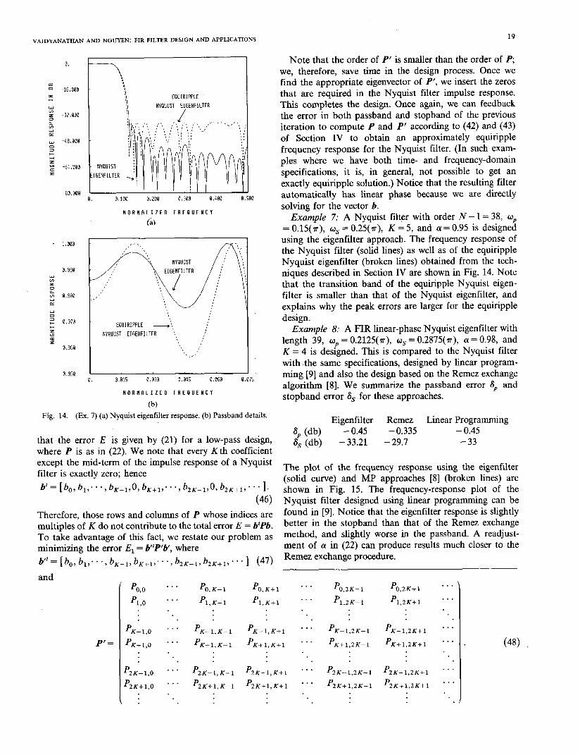
Example 7: A Nyquist filter with order N - 1 = 38, wp = 0.15(a), ws = 0.25(g), K = 5, and (Y = 0.95 is designed using the eigenfilter approach. The frequency response of the Nyquist filter (solid lines) as well as of the equiripple Nyquist eigenfilter (broken lines) obtained from the techniques described in Section IV are shown in Fig. 14. Note that the transition band of the equiripple Nyquist eigenfilter is smaller than that of the Nyquist eigenfilter, and explains why the peak errors are larger for the equiripple design.

Example 8: A FIR linear-phase Nyquist eigenfilter with length 39, C+ = 0.2125(r), ws = 0.2875(n), cu = 0.98, and K = 4 is designed. This is compared to the Nyquist filter with -the same specifications, designed by linear programming [9] and also the design based on the Remez exchange algorithm [8]. We summarize the passband error 8, and stopband error 6, for these approaches.

Eigenfilter Remez Linear Programming $, (db) - 0.45 - 0.335 - 0.45 8, (db) - 33.21 - 29.7 -33

The plot of the frequency response using the eigenfilter (solid curve) and MP approaches [8] (broken lines) are shown in Fig. 15. The frequency-response plot of the Nyquist filter designed using linear programming can be found in [9]. Notice that the eigenfilter response is slightly better in the stopband than that of the Remez exchange method, and slightly worse in the passband. A readjust- ment of (Y in (22) can produce results much closer to the Remez exchange procedure.

pO, K-l P 0, Kil

P l,K-1 P l,K+l

P * K-l,K-1 P . K-l,K+l

P K+l,K-1 P K+l,K+l

p2K-;,K-l ‘2K-l,K+l

P 2K+l,K-1 P 2K+l,K+l

. . . P 0,2K-1

. . . P 1,2K-1

. . . P . K-1,2K-1

. . . P K+1,2K-1

. . . p2K-;,2K-l

. . . P 2K+1,2K-1

P 0,2K+l ..’

P 1,2K+l ***

P . * ’ * K-1,2K+l

P * ’ * K+1,2K+l

p2K-;,2K+l . ’ ’

P ’ * ’ 2K+1,2K+l

(48)

EIGENFILTER RDlEZ EXCHANGE

APPROACH ALGORITHM

\

0.100 0.200 0.300 0.400

NORMRLIZELI FREOUENCY

(4

0.5011

-1.000 1 I 0. 0.022 0.043 0.065 0.086 0.108

NORRRLIZED FREEUENCY

C-9

Fig. 15. (Ex. 8) (a) Magnitude response of Nyquist filter, designed using the eigenfilter approach and Remez exchange algorithm. (b) Passband details.

IEEE TRANSACTIONS ON CIRCUITS AND SYSTEMS, VOL. CA:%34, NO. 1, JANUARY 1987

this section, we impose the flatness constraints at any frequency in the passband using the eigenfilter approach.

Consider an even-order filter (type 1) H(z) of order N - 1. Its amplitude response can be written as a function of sin* (w/2), i.e.,

Ho(@) = 5 b,cosnw = f cncoP (;) n=O n=O

= fJ d,sin*“(t). n=O

(4%

Suppose the first L + 1 coefficients (except do) of H,(ej”) are zero, i.e.,

H,( eio) = do + dL+I sin2(L+‘) i 1 t

+d

Clearly, the first 2L + 1 derivatives of H,(e@) are zero at w = 0, i.e.,

d(k) dw,H,(ej,) = 0, l<k:<2L+l. (51)

This fact suggests a procedure to design filters with flatness constraints using the eigenfilter approach. Defining

d=[d, d, d,...d,-, d,]’ N-l even (52)

and

u= [l sin*(f) sin4(:) ... sin2(Mp1)(t) sin2M(t)]’

we then have

Ho( ej”) = d’v.

To achieve a 2 L + 1 degree of flatness at o = 0, we define new sequences d’ and u’ as

d’= [do d,,, dL+* *. . d,-, d,]’

u’= 1 sinz(Lil)( ff) sin*CL-+*)( Tf) . . . sin*CM-ll( t) c&*M( ff)] ‘.

(53)

(54

(55)

(56)

VI. EIGENFILTERS THAT HAVE ARBITRARY DEGREE OF FLATNESS AT ANY GIVEN FREQUENCY IN THE

PASSBAND

Incorporating this into (15) and (20), we have the new objective function E = (d’)Pd’, where P is as in (22) with

Digital FIR filters with a maximally flat frequency response at frequency w = 0 have been studied by Herrmann [21], Kaiser [22], and Vaidyanathan [23]. FIR

(57)

(58) filters of this class find applications in several filtering problems, as pointed out by Kaiser and Steiglitz [24). In where 1’ = [l 0 0 . . . 01’. Now if we find the eigen-


vector corresponding to the minimum eigenvalue of P, the resulting response has the desired flatness at w = 0. We can easily generalize this approach when the flatness constraints are required at an arbitrary frequency. Thus, the frequency w. at which the first 2 L + 1 derivatives are zero can be varied by expanding H,( ej”) in terms of sin*” (w - wo/2) in (49).

VII. EIGENVECTORCOMPUTATIONANDRELATED ISSUES

A major part of the design time for our method is spent in the computation of the eigenvector. Since we are interested in only one eigenvector (corresponding to an extremal eigenvalue), this computation can be done effi- ciently (without invoking general methods such as the QR technique [29]). It is well known [25], [26] that to compute the dominant eigenvalue and its corresponding eigenvector, the iterative power method is simple and fast if the ratio 1X,/X,-,] is large where X, are the eigenvalues of P with

IX,1 2 IA,-,1 > * * * 2 IX,I > IhJ. At the k + lth iteration of the power method, a vector

xk+i is computed from the previous iterate xk as

Yk+l= pxk (594

xk+l = Yk+l/llYk+lll (59’4

where ~~o~~ denotes the L, norm of vector ~1. The difference between xk and xk+i, defined by IIxk+i - xkll is compared to a prescribed small constant Q, and if

IIxk+l - Xkll < c (60) then xk+i is a good approximation of the eigenvector corresponding to the maximum eigenvalue. A typical value for E is about 1.0 x 10p6.

We, however, wish to compute the minimum eigenvalue and its corresponding eigenvector. In other words, at each iteration, we would like to compute *

X k+l= P-h,. (61) Given xk, we would like to find xk+i without inverting P-l. Rewrite (61) as

Xk = PXkhl. (62)

It is well known [25], [26] that a real, symmetric, and positive-definite matrix P can be decomposed into

P=LL’ (63) where L is a real lower triangle matrix. Equation (62) then becomes

Xk = LLtxk+l. (64 Let

Then

0 k+l= Ltxk+l*

Xk = Lvk+,.

(65)

(66)

We can find vk+ i in (66), given xk and L, by recursively solving a set of linear equations. Let lij be the element in the ith row and jth column of L; then we can show that

uk+l(n)=f ~k(~)-~~~~~j”k+~(~)). i

(67) nn

Since P is positive-definite, I,,,, in (67) are evidently non- zero. Using (67), we first solve for uk+i(0) and solve recursively for all uk+i(n) for 1~ n < N- 1, where N is the dimension of L. (In (67), xk(n) denotes the nth element of vector xk.) It takes N(N - 1)/2 multiplications, N divisions, and N( N - 1)/2 additions to compute vk ‘t i. Similarly, we can find xk+i in (65) given vk+i and L. The total time required per iteration is thus

0, + L) N(N-1)

2 +Nt, x2 1

= (t,+t,)N(N-1)+2Nt,

where t =, t m, t, are, respectively, the required computer times for addition, multiplication, and division.

Note that the speed of convergence depends on the ratio A,/X, since we are dealing with P-’ rather than P. Instead of proceeding as in (65) and (66) one could invert P beforehand, store it as Q, and then perform the iteration

Yk+l= f&k @a)

xk+l = Yk+l/ll Yk+lll* (68b)

The operation (68a) requires N * multiplications and N( N - 1) additions, and the time required for this is

t,N(N-l)+ t,N*

which is nearly the same as the time required for per- forming (65) and (66). However, there is an overhead cost associated with the computation of Q.

Example 9: Table I indicates a comparison of design time for half-band filters, using the eigenfilter approach and the Remez exchange approach, for various tolerances. The ratio X,/X, and the number of iterations required for eigenvector computation are also given. We observe that X*/h is large and, hence, the number of iterations for eigenvector computation is impressively small for all the entries in Table I.

We also summarize below the design time, number of iterations, X,/A,, a,, and S, for the Nyquist filter designed in Example 8 (solid curve in Fig. 15):

CPU time Number of X,/X, 6, (db) 6, (db) (se4 iterations 3.9 3 792 - 0.45 -33

Our experience based on a large number of design ‘examples has convinced us that the ratio A,/& is large in all practical cases. Accordingly, the eigenvector computation never creates any numerical or stability problems and is invariably fast. Single precision arithmetic is found to be sufficient in all design examples.

22 IEEE TRANSACTIONS ON CIRCUITS AND SYSTEMS, VOL. CAS-34, NO. I, JANUARY 1987

TABLE1 COMPARISON OF THE EIGENFILTER AND THE REMEZ EXCHANGE

APPROACHES IN THE HALF-BAND FILTER DESIGNS

EIGENFILTER REMEZ EXCEANGE

% N-l 61

.4* 14 0.054

.42r 18 0.0403

.425r 22 0.0317

.435r 26 0.0245

.435n 30 0.0188

.44x 34 0.0142

,445~ 42 0.00612

,445~ 46 o.Oi!604

.47* 56 0.0164

.47x 62 0.0146

.47lr 66 0.0124

.47x 74 O.W9+54

.41x 76 0.00642

.4725x 90 o.OQ607

.4725x 98 0.00447

.475x 130 0.00135

,491 202 o.OaO6

2 Number of CPU time iterations (4

62 4 0.3

152 4 0.4

309 3 0.) ’

614 3 0.7

lOQ0 3 0.8

1687 3 1.0

4566 3 1.4

6634 3 1.5

2230 3 2.6

2610 3 2.6

3507 3 2.9

5176 3 3.6

6150 3 3.9

13117 3 5.1

19562 3 5.9

91752 3 10.0

21069 3 24.5

N-l

10

14

16

22

26

30

36

42

54

56

62

66

70

76

90

122

162

61 CPU (sec.)

0.0465 0.4

0.0402 0.5

0.0265 0.6

0.0233 0.7

0.0146 0.6

0.0120 0.9

0.0072 1.5

0.0049 1.4

0.017 1.6

0.0137 2.5

0.011 2.2

0.009 2.6

0.0073 2.6

0.00672 3.7

0.00376 4.1

0.0014 6.6

0.00104 12.4

n-l is the required order for peak passband ripple S, and transition band- width 2(lr/2- nr).

There exist some recent methods for computing eigen: vectors (corresponding to extremal eigenvalues) based on gradient techniques [30]. These could prove to be even faster than the iterative power method, but we have not studied this possibility in the context of our paper.

VIII. CONCLUDING REMARKS

In this paper, we have formulated linear-phase FIR design problems in the form of eigenproblems. The filter coefficients are computed from eigenvectors of certain matrices which represent the specification requirements. A set of specification requirements directly leads to the Kaiser-window frequency response. Eigenfilters can be designed in such a way that various time-domain recluire- ments are simultaneously taken into account. By means of an error-feedback mechanism, an iterative method also has been presented that leads to near-equiripple eigenfilters. The eigenfilter approach is also used to design Nyquist filters and filters with flatness constraints in the frequency domain. In conclusion, a wide variety of specifications can be taken into account by the eigenfilter .approach. The design examples presented and the design times compare favorably with several other methods reported in the litera- ture.

ACKNOWLEDGMENT

The authors are grateful to the reviewers for useful comments and suggestions. Also, valuable discussions with Quan Phuong Hoang, graduate student at Caltech, on computational aspects are eratefullv acknowledeed.

VI

PI

131

[41

[51

161

171

[81

191

WI

WI

WI

1131

P41

1151

WI

[I71

V-51

P91

PO1

WI

P21

v31

~241

v51

WI

~271

WI

~291

REFERENCES

J. H. McClellan and T. Parks, “A unified approach to the design of optimum FIR linear-phase digital filte:rs, ’ IEEE Trans. Circuit Theory, vol. CT-20, pp. 697-701, Nov. 1973. D. W. Tufts and J. T. Francis, “Designing digital lowpass filters: Comparison of some methods and criteeria,” IEEE Trans. Audio Electroucoust., vol. AU-18, pp. 487-494, Dec. 1970. W. C. Kellogg, “Time domain design of nonrecursive least mean- square digital filters,” IEEE Trans. Audio Electroacoust., vol. AU-20, pp. 155-158, June 1972. D. C. Farden and L. L. Scharf, “Statistical design of nonrecursive digital filters,” IEEE Trans. Acoust., Speech, Signal Process., vol. ASSP-22, pp. 188-196, June 1974. Y. C. Lim and S. R. Parker, “Discrete coefficient FIR digital filter design based upon an LMS criteria,” IEEE Trans. Circuits Syst., vol. CAS-30, pp. 723-739, Oct. 1983. V. K. Jain and R. E. Crochiere, “Quadrature mirror filter design in the time-domain,” IEEE Trans. Acoust., Speech, Signal Process., vol. ASSP-32, pp. 353-361, Apr. 1964. L. R. Rabiner and B. Gold, Theory and Application of Digitul Signal Processing. Englewoods Cliffs, NJ: Prentice-Hall, 1975. F. Mintzer, “On half-band, ‘third-band and Nth band FIR filters and their design,” IEEE Trans. Acoust., Speech, Signal Process., vol. ASSP-30, pp. 734-738, Oct. 1982. J. K. Liang, R. J. P. Defigueiredo, and F. C. Lu, “Design of optimal Nyquist, partial response, Nth band, and nonuniform tap spacing FIR digital filters using linear programming techniques,” IEEE Trans. Circuits Svst.. vol. CAS-32. no. 386-392. Am. 1985. A. Antoniou, Digital ‘Filters: Analysis a’nd Design. ’ Nkw York: McGraw-Hill. 1979. P. P. Vaidyanathan, “Design and implementation of digital FIR filters” in Handbook of Digital Signal Processing, D. F. Elliott, Ed. New York: Academic Press. D. W. Burlage, R. C. Houts, and G. 1,. Vaughn, “Time-domain design of frequency-sampling digital filters for pulse shaping using linear programming techniques,” IEEE Trans. Acoust., Speech, and Signal Process., vol. ASSP-22, pp. 1130-185, June 1974. K. Feher, M. El-Torky, and R. DeCristofaro, “Optimum pulse shaping application of binary transversal filters used in satellite communication,” Radio Electron. Eng., vol. 47, no. 6, pp. 249-256, June 1977. K. Feher and R. DeCristofaro,, “Transversal filter design and application in satellite commumcation,*’ IEEE Trans. Commun., vol. COM-24, pp. 1262-1268, Nov. 1976. K. Nakayama and T. Mizukami, “A new IIR Nyquist filter with zero intersymbol interference and its frequency response approximation,” IEEE Trans. Circuits Syst., vol. CAS-29, pp. 23-34, Jan. 1982. J. Makhoul, “On the eigenvectors of symmetric Toeplitz matrices,” IEEE Trans. Acourt., Speech, Signal Process., vol. ASSP-29, pp. 868-872, Aug. 1981. S. M. Kay and S. L. Marple, Jr., “Spectrum analysis-A modern perspective,” Proc. IEEE, vol. 69, pp. 1380-1419, Nov. 1981. J. F. Kaiser, “Nonrecursive digital filter design using the I,-sinh window functions,” in Proc. 1974 IEEE Svmp. Circuits Syst., Apr. 1974, pp. 20-23.

_

B. Nobel and J. W. Daniel, Applied Linear Algebra. Englewood Cliffs. NJ: Prentice-Hall. 1977. L. R. kabiner, “Approximate design relationships for low-pass FIR filters,” IEEE Trans. Audio Electroacourr., vol. AU-21, pp. 456-460, Oct. 1973. 0. Hermann, “On the approximation problem in nonrecursive digital filter design,” IEEE Trans. Circuit Theory, vol. CT-18, pp. 411-413, May 1971. J. F. Kaiser, “Design subroutine (MXFLAT) for symmetric FIR low-pass digital filters, with maximally-flat pass and stopbands,” in {roxnns for Digital Signal Processing. New York: IEEE Press,

P. P. Vaidyanathan, “Optimal design of linear-phase FIR digital filters with very flat passbands and equiripple stopbands,” IEEE Trans. Circuits Syst., vol. CAS-32, pp. 904-917, Sept. 1985. J. F. Kaiser and K. Steiglitz, “Design of FIR filters with flatness constraints,” in IEEE Znt. Conf. Acoust., Speech, Signal Process. (Boston, MA), Apr. 1983, pp. 197-199. J. N. Franklin, Matrix Theory. Englewood Cliffs, NJ: Prentice- Hall, 1968. G. W. Stewart, Introduction to Matrix Computation. New York: Academic Press, 1973. C. Charalambous, “Acceleration of th’e least jth algorithm for minimax optimization with engineering applications,” Math. Pro- gram., vol. 17, pp. 270-297, 1979. C. Charalambous and A. Antoniou, “Equalization of recursive digital filters,” Proc. Inst. Elec. Eng., pt. G, vol. 127, pp. 219-225, 1980. J. H. Wilkinson, The Algebraic Eigenualue Problem. London: Ox- ford University Press, 1965.


[30] Y. H. Hu and P. K. Chou, “Effective adaptive Pisarenko spectrum Electrical Engineering. His main research interests are in digital signal estimate,” in Proc. IEEE Int. Conf. Acoust., Speech, Signal Pro- processing, linear systems, and filter design. cess. (Tokyo, Japan), 1986, pp. 577-580.

[31] R. E. Crochiere and L. R. Rabiner, Multirate Digital Signal Dr. Vaidyanathan served as the Vice-Chairman of the Technical Pro-

Processing. En lewood Cliffs, NJ: Prentice-Hall. gram Committee for the 1983 IEEE International Symposium on Circuits

[32] P. P. Vaidyanat a an and T. Q. Nguyen,“A ‘trick’ for the design of and Systems. He currently serves as an Associate Editor for the IEEE

FIR half-band filters,” IEEE Trans. Circuits Sysr., to be published. TRANSACTIONS ON CIRCUITS AND SYSTEMS. He was the recipient of the Award for Excellence in Teaching at the California Institute of Technol- ogy for 1983/84. He was also a recipient of the NSF’s Presidential Young Investigator Award, starting from the year 1986.

P. P. Vaidyanathan (S’SO-M’83) was born in Calcutta, India, on October 16, 1954. He received the B.Sc. (with honors) degree in physics, and the B. Tech. and M. Tech. degrees in radio- physics and electronics from the-University of Calcutta, India, in 1974, 1977, and 1979, respectively, and the Ph.D. degree in electrical and computer engineering from the University of California, Santa Barbara, in 1982.

He was a Postdoctoral Fellow at the Univer- sity of California, Santa Barbara, from Septem-

ber 1982 to February 1983. Since March 1983, he has been with the California Institute of Technology, Pasadena, as an Assistant Professor of

Truong Q. Nguyen (s’85) was born in Saigon, Vietnam. on November 2, 1962. He received the B.S. (with honors) and M.S. degrees from the California Institute of Technology in electrical engineering in 1984 and 1985, respectively, and is currently pursuing the Ph.D. degree at the same institution. He is a recipient of a fellowship from Aerojet General for advanced studies. Mr. Nguyen’s main research interests are in digital signal processing and filter designs. He is a member of Tau Beta Pi and Eta Kappa Nu.

cas-34, no. 1, january eigenfilters: a new approach to least-squares fir filter design and...

Documents