University of Nebraska - LincolnDigitalCommons@University of Nebraska - Lincoln

Journal of Actuarial Practice 1993-2006 Finance Department

1999

CARVM and NAIC Actuarial Guidelines 33 & 34Keith P. SharpUniversity of Waterloo, Canada, SharpWaterloo@compuserve.com

Follow this and additional works at: http://digitalcommons.unl.edu/joap

Part of the Accounting Commons, Business Administration, Management, and OperationsCommons, Corporate Finance Commons, Finance and Financial Management Commons, InsuranceCommons, and the Management Sciences and Quantitative Methods Commons

This Article is brought to you for free and open access by the Finance Department at DigitalCommons@University of Nebraska - Lincoln. It has beenaccepted for inclusion in Journal of Actuarial Practice 1993-2006 by an authorized administrator of DigitalCommons@University of Nebraska -Lincoln.

Sharp, Keith P., "CARVM and NAIC Actuarial Guidelines 33 & 34" (1999). Journal of Actuarial Practice 1993-2006. 84.http://digitalcommons.unl.edu/joap/84

Journal of Actuarial Practice Vol. 7, 1999

CARVM and NAIC Actuarial Guidelines 33 & 34

Keith P. Sharp*

Abstract

Annuity valuation under the NAIC Standard Valuation Law is determined according to methods different from those methods used for life insurance. The CARVM assumption of effiCient policyholder selection is clarified under NAIC Actuarial Guidelines 33 and 34 to allow for non-elective (e.g., death) ben­efits. In particular, Actuarial Guideline 34 is oriented toward variable annuities and prescribes methods to be used in the presence of a minimum guaranteed death benefit. In this paper these methods are examined and illustrated with examples.

Key words and phrases: annUity, elective benefit, valuation, reserves

1 Introduction

In the previous article in this volume, Sharp (1999) explained the calculations involved in determining annuity reserves under the com­missioners annuity reserve valuation method (CARVM). These reserves are calculated by a method different from that used for insurance re­serves (American Academy of Actuaries, 1997). CARVM assumes that for elective benefits such as surrender, the policyholder will select with 100 percent efficiency the best time to make the election, if the com­parisons are made using the company's valuation rate of interest. More

* Keith Sharp, F.SA, Ph.D., is an associate professor at the University of Waterloo, Canada. He has worked as an actuary for penSion consulting firms in Canada and Australia and for an insurance company in Britain. His papers have appeared in various journals, including Transactions of the Society of Actuaries, Insurance: Mathematics and Economics, journal of Risk and Insurance and this journal.

Dr. Sharp's address is: Department of Statistics & Actuarial SCience, Univer­sity of Waterloo, Waterloo ON N2L 3Gl, CANADA. Internet address: SharpWater­loo@compuserve.com

126 Journal of Actuarial Practice, Vol. 7, 1999

concisely, this is the worst time for the insurance company. In some simple cases the CARVM reserve is calculated using formulas contain­ing no probabilities.

In this paper we consider the treatment of annuities with a (non­elective) benefit on death under National Association of Insurance Com­missioners (NAIC) Actuarial Guideline (AG) 33 (NAIC, 1998). In two examples we consider the case of a fixed (nonvariable) annuity. The treatment is extended in later examples to the valuation under NAIC Actuarial Guideline 34 of variable annuities with a minimum guaran­teed death benefit (MGDB).

2 Actuarial Guideline 33

After its 1976 introduction there was some disagreement about how CARVM should be applied to the situation where there were potentially elective and non-elective (e.g., death) benefits. After the issue of Actu­arial Guideline 33 (formerly GGG) (see, e.g., Lalonde, 1995) there contin­ued to be some confusion on this issue. The method of using CARVM in complicated situations, however, now has been largely resolved.

At its September 1995 meeting, the NAIC Life and Health Actuarial Task Force interpreted Actuarial Guideline 33 to require consideration of integrated benefits in the CARVM stream(s). Here integrated refers to the consideration of the present value of benefit streams under which certain proportions of policyholders are dying and the remaining poli­cyholders are selecting the optimum time of surrender. Under the re­vised version of Actuarial Guideline 33 effective December 31, 1998, benefits are classified as either elective or non-elective. Each possible set of elections then is conSidered. This may result in a large tree of possible sets of elections.

For example, there may be a policy provision for annual surrender of up to 10 percent of the annuity value without imposition of a back­end load (surrender charge). One possible branch of the tree would correspond to a 10 percent surrender at the end of policy year one, a 5 percent surrender at the end of policy year two, a 10 percent surrender at the end of policy year three, etc. Typically one can use linearity to cut the number of branches to be tested. In other words, the reserve candi­date is likely to be a linear function of the surrender proportion. Hence, the reserve candidate is a monotonic (increasing or decreasing) function of the surrender proportion. In this case the maximum corresponds to either the lowest or the highest possible surrender proportion. In this example, the CARVM maximum would likely correspond to either a 0

Sharp: Actuarial Guidelines 33 & 34 127

percent or 10 percent surrender at the end of year two, not a 5 percent surrender. Superimposed on this structure would be the probabilities of death, a non-elective benefit for which the use of expected values is appropriate. A valuable intuitive analysis of complicated situations like this is given by Backus (1998).

3 Example 1 : Simple CARVM with Zero Deaths

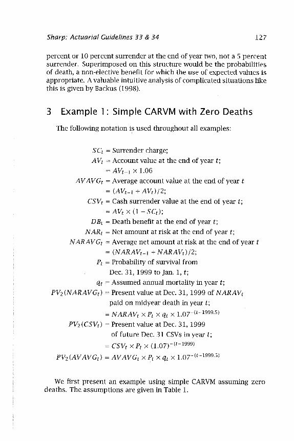
The following notation is used throughout all examples:

SCt = Surrender charge; AVt = Account value at the end of year t;

= AVt-l x 1.06

A V AV Gt = Average account value at the end of year t = (AVt-l + AVd/2;

CSVt = Cash surrender value at the end of year t; = AVt x (1- SCt);

DBt = Death benefit at the end of year t; N ARt = Net amount at risk at the end of year t;

N ARA V Gt = Average net amount at risk at the end of year t

= (NARAVt-l + NARAVd/2;

Pt = Probability of survival from

Dec. 31, 1999 to Jan. 1, t; qt = Assumed annual mortality in year t;

PV2(NARAVGt) = Present value at Dec. 31,1999 of NARAVt paid on midyear death in year t;

= NARAVt X Pt x qt x 1.0r(t-1999.5)

PV2(CSVt) = Present value at Dec. 31, 1999 of future Dec. 31 CSVs in year t;

= CSVt x Pt x (1.07)-(t-1999)

PV2(AV AVGd = AV AVGt x Pt x qt x 1.0r(t-1999.5)

We first present an example using simple CARVM assuming zero deaths. The assumptions are given in Table 1.

128 Journal of Actuarial Practice, Vol. 7, 7999

Table 1 Valuation Assumptions for

A Single Premium Deferred Annuity (Fixed) Issue date: January 1,1998 Single premium: $60,000 Accumulation

Guaranteed: Actual for 1998 and 1999:

Death benefit: Front end load: Back end load

Policy year 1: Policy year 2: Policy year 3: Policy year 4:

Valuation date: Valuation mortality rate

Policy year 1: Policy year 2: Policy year 3: Policy year 4:

Valuation interest rate:

6 percent per annum 6 percent per annum $100,000 o percent

8 percent 4 percent o percent o percent December 31, 1999

0.000 0.000 0.000 0.000 7 percent per annum

Specifically, assume a January 1, 1998 issue of a $60,000 single pre­mium deferred annuity credited with a guaranteed 6 percent per an­num. In other words, the account value (fund value) visible to the poli­cyholder is credited at a rate of at least 6 percent per annum.

Assume that the contract specifies that the policy matures after four years. To motivate a later discussion of a variable minimum guaran­teed death benefit we discuss a policy with (perhaps unrealistically) a $100,000 minimum death benefit.

A valuation is to be performed on December 31, 1999, and we need to consider possible surrender on December 31, 1999, December 31, 2000, or December 31,2001. The immediate December 31, 1999 cash surrender value (CSV) forms a floor for the CARVM reserve. The two dates December 31, 2000 and December 31, 2001 represent two candi­dates for the status of maximum present value at December 31, 1999.

Sharp: Actuarial Guidelines 33 & 34 129

The CARVM reserve is the greater of these two but with a floor of the immediate CSV. The reserve calculations are shown in Table 2.

Surrender on December 31, 1999

We have accumulation at 6 percent per annum so AVt = AVt-l x 1.06, where AVt is the account value at the end of year t. By December 31, 1999 the account value (Rows (3) and (4) of Table 2) has grown to 60,000 X 1.062 = $67,416. An immediate surrender would be for 67,416 x (1-0.04) = $64,719, which is a floor to the CARVM reserve.

Surrender on December 31, 2000

A surrender at December 31, 2000 is projected to give a CSV of 60,000 x 1.063 = $71,461 and hence a reserve candidate at December 31,1999 of 71,461/1.07 = $66,786.

Surrender on December 31, 2001

A surrender at December 31, 2001 is projected to give a CSV of 60,000 x 1.064 = $75,749 and hence a reserve candidate at December 31,1999 of 75,749/1.072 = $66,162.

Table 2 Reserve Using Assumption of Zero Mortality

Policy year from Jan. 1, (t)

1998 1999 2000 2001

SCt: 8% 4% 0% 0% AVt-l at Jan. 1: 60,000 63,600 67,416 71,461 AVt at Dec. 31: 63,600 67,416 71,461 75,749 AVAVGt: 61,800 65,508 69,438 73,605 CSVt: 58,512 64,719 71,461 75,749 PV2(CSVr): 64,719 66,786 66,162

CARVM Maximum of the Candidates:

The largest of these candidates is $66,786, which is the CARVM re­serve at December 31, 1999 if we are assuming zero mortality. Here we

130 Journal of Actuarial Practice, Vol. 7, 7999

are using strict noncontinuous CARVM, examining only surrenders on the last day of each contract year.

We assume that no decision has been made touse continuous CARVM, that is, to use the maximum over all possible days of surrender. New York requires the use of continuous CARVM. Many actuaries (includ­ing the author) believe that continuous CARVM gives more appropriate reserves. In this case a surrender on January 1, 2000, the day after val­uation, would give a CSV of $67,416 because the surrender charge is then zero. In reality, it would be preferable to use the $67,416 as floor to the standard CARVM reserve which otherwise is $66,786.

4 Example 2: Assuming Non-Zero Deaths

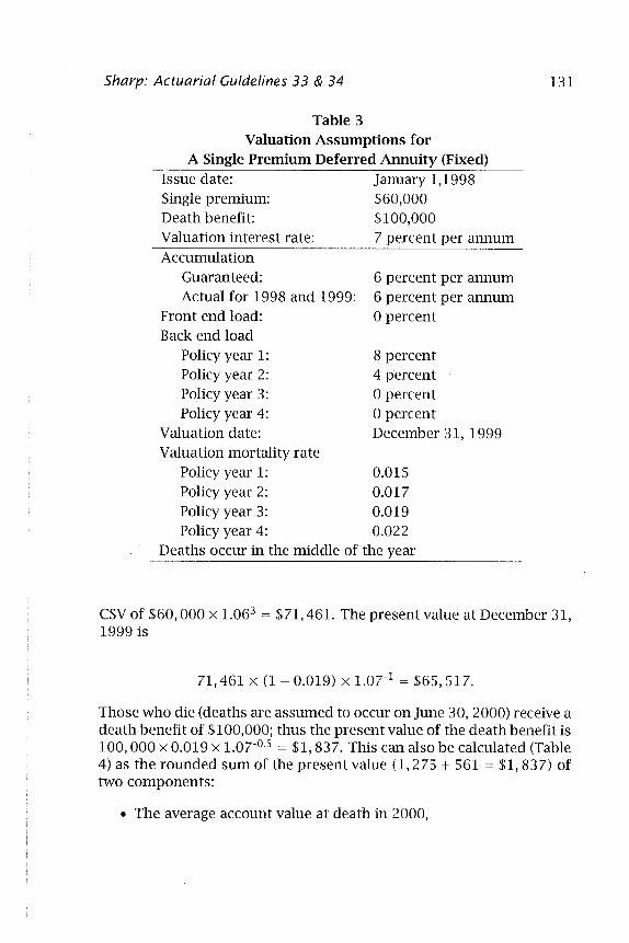
Let us extend our example to highlight the elective/non-elective dis­tinction. Now the previous contract is revalued assuming nonzero deaths, as indicated below. The fixed $100,000 death benefit is now integrated into the reserve calculation. The assumptions are given iIi Table 3.

The reserve will consist mainly of the present value of the elected cash surrender value (CSV), but we add also the value of deaths by those who otherwise would make the optimal selection. Surrender on Decem­ber 31, 2000 or 2001 gives two candidates for the status of maximum present value at .December 31, 1999. With consideration of the floor of the immediate December 31, 1999 CSV we have three candidates for the CARVM reserve: surrender on December 31, 1999, surrender on December 31,2000, or surrender on December 31, 2001.

Surrender on December 31, 1999

Here we consider an immediate surrender on the valuation day. As in Table 2, we have a CSV of $64,719. Under New York (continuous) CARVM (New York Insurance Law, Section 4217(6)(D» we consider also a surrender a day later, on January 1, 2000. Under noncontinuous CARVM, however, we do not consider a January 1, 2000 surrender even though that would give a higher value because the 4 percent load has then become zero. The December 31,1999 candidate to be the CARVM maximum is $64,719 ..

Surrender on December 31, 2000

A proportion (1 - 0.019) of the policyholders survives to the end of calendar year 2000 and under this candidate they then surrender for a

Sharp: Actuarial Guidelines 33 & 34

Table 3 Valuation Assumptions for

A Single Premium Deferred Annuity (Fixed) Issue date: Single premium: Death benefit: Valuation interest rate: Accumulation

Guaranteed: Actual for 1998 and 1999:

Front end load: Back end load

Policy year 1: Policy year 2: Policy year 3: Policy year 4:

Valuation date: Valuation mortality rate

January 1,1998 $60,000 $100,000 7 percent per annum

6 percent per annum 6 percent per annum o percent

8 percent 4 percent o percent o percent December 31,1999

Policy year 1: 0.015 Policy year 2: 0.017 Policy year 3: 0.019 Policy year 4: 0.022

Deaths occur in the middle of the year

131

CSV of $60,000 x 1.063 = $71,461. The present value at December 31, 1999 is

71,461 x (1 - 0.019) X LOTI = $65,517.

Those who die (deaths are assumed to occur on June 30, 2000) receive a death benefit of $100,000; thus the present value of the death benefit is 100,000 x 0.019 x 1.07-0.5 = $1,837. This can also be calculated (Table 4) as the rounded sum of the present value (1,275 + 561 = $1,837) of two components:

• The average account value at death in 2000,

l32 Journal of Actuarial Practice, Vol. 7, 7999

(67,416 + 67,416 x 1.06)/2 = $69,438,

with prese.nt value

69,438 x 0.019 x (1.07)-0.5 = $1,275.

• The average excess of the death benefit over the average account value,

(100,000-69,438) x 0.019 x LOro.s = $561.

The Table 4 approach is comparable to that used later in valuing a min­imum guaranteed death benefit.

Hence the total value of this candidate is 65,517 + 1,837 = $67,354.

Surrender on De~ember 31, 2001

A proportion (1 - 0.019) x (1 - 0.022) of the policyholders survives calendar years 2000 and 2001 and under this candidate they then sur­render for a CSV of $60,000 x 1.064 = $ 75,749. The present value at December 31, 1999 is

75,749 x (1 - 0.019) x (1 - 0.022) x (1.07)-2 = $63,477.

Those who die during 2001 (on June 30, 2001) receive $100,000; thus the present value of the year 2001 death benefit is

100,000 x (1 - 0.019) x 0.022 x 1.07-1.5 = $1,949.

Some fellow cohorts of those surrendering on December 31, 2001 die also in 2000, so we add that present value also (above), 1,837 + 1,949 =

$3,787, rounded to agree with the 1,076 + 2,711 = $3,787 of Table 4. Hence the total value of this candidate is 63,477 + 3,787 = $67,264.

Table 4 Integrated Reserve Including Fixed $100,000 Death Benefit

Policy year commencing Jan. 1 (t): 1998 1999 2000 2001 2002 CSVt at Dec. 31: 58,512 64,719 71,461 75,749 DBt-l atJan. 1: 100,000 100,000 100,000 100,000 DBt (death benefit) at Dec. 31: 100,000 100,000 100,000 100,000 NARt-l (benefit top-up) at Jan. 1: 44,800 38,944 32,584 28,539 NAR t (benefit top-up) at Dec. 31: 41,488 35,281 28,539 24,251 NARAVGt (benefit top-up): 43,144 37,112 30,562 26,395 qt: 0.015 0.017 0.019 0.022

Pt= 1.000 0.981 0.959 PV2(NARAVGt)*: 561 515 PV2(AVAVGd: 1,275 1,435

CUMPV2(NARAVGt ) = I~=1999(NARAVGs): 561 1,076

CUMPV2(AVAVGd = I~=1999(AVAVGs): 1,275 2,711 PV2(CSVd**: 64,719 65,517 63,477 Total-Integrated reserve (VfNT): 64,719 67,354 67,264

Notes: V£NT is the maximum of this row of candidates Vf,tND, and is the sum of the previous three rows of this table.

*PVz(NARAVGt) = NARAVG t x Pt x qt x 1.07-(t-1999.5).

** PVz (CSVt) at Dec. 31, 1999 of Dec. 31 CSV = CSVt x Pt x 1.07-(t-1999.5).

V) ::s­li:)

~ ):,. r,

2 li:)

"'" ~ ~ ~ ~ 3i' (\) VI

W W

~ W ~

r-­W W

l34 Journal of Actuarial Practice, Vol. 7, ] 999

CARVM Maximum of the Candidates

Hence we have for our valuation at December 31, 1999 three possible elections for surrender:

• December 31, 1999: $64,719

• December 31, 2000: $67,354

• December 31, 2001: $67,264.

For this fixed annuity under CARVM, in marked contrast with life insur­ance valuation, we use the greatest of these three candidates, $67,354, as our CARVM reserve at December 31,1999.

5 Example 3: Minimum Guaranteed Death Bene­fits

Under certain annuity designs, often called variable annuities, the account value, and hence the CSV, varies with the investment perfor­mance of the underlying assets. Commonly the contract specifies that on death the benefit will be the greater of the account value and a min­imum guaranteed death benefit.

Consider a single premium variable annuity with valuation assump­tions given in Table 5. We will look at various possible contract provi­sions defining the death benefit. The benefit on surrender on August 14, 2000 will be the account value net of a 4 percent back-end load:

10,000 x (1 + 0.12) x (1 - 0.l3) x (1 - 0.04) = $9,354.

If the contract provisions provide for the surrender charge to be waived on death, then the benefit on death on August 14, 2000 is:

10,000 x (1 + 0.12) x (1 - 0.l3) = $9,744.

If on death the surrender charge is waived and there is a minimum ben­efit of the return of premium (one possible design of minimum guaran­teed death benefit), the benefit on death on August 14, 2000 is $9,744 with a floor of $10,000; hence the death benefit is $10,000.

lf on death the surrender charge is waived and there is an annual reset of the minimum guaranteed death benefit on the policy anniver­sary, the benefit on death on August 14, 2000 is $11,200. It was reset

Sharp: Actuarial Guidelines 33 & 34

Table 5 Valuation Assumptions for

A Single Premium Deferred Annuity (Variable) Issue date: August IS, 1998 Single premium: $10,000 Surrender charge

During policy year 1: During policy year 2: During policy year 3: Thereafter:

Actual credited rate

6 percent 4 percent 2 percent o percent

August 15,1998 to Aug 14, 1999: 12 percent August 15,1999 to Aug 14, 2000: -13 percent August IS, 2000 to Aug 14, 2001: -8 percent August IS, 2001 to Aug IS, 2002: 2 percent

135

August 15,1999 to the then fund value 10,000 x (1 + 0.12) = $11,200 and at August IS, 2000 will be set to 11,200 x (1 - 0.13) = $9,744.

If on death the surrender charge is waived and there is an annual ratchet of the minimum guaranteed death benefit on the policy anniver­sary, then the benefit on death on August 14, 2001 is $11,200. On Au­gust 15,1999 the minimum guaranteed death benefit was ratcheted up to the then fund value 10,000 x (1 + 0.12) = $11,200 and was left unchanged at August IS, 2000-the ratchet means that the minimum guaranteed death benefit cannot be reduced.

The design of the minimum guaranteed death benefit can vary widely; the above set of illustrations is only a small subset of the possible de­signs. Actuarial Guideline 34 is intended to apply to all such designs.

6 NAIC Actuarial Guideline 34

AG 34 (NAIC, 1998) requires that minimum guaranteed death ben­efits be projected by assuming an immediate drop in the values of the assets supporting the variable annuity contract, followed by a subse­quent recovery in asset values at a net assumed return until the ma­turity of the contract. The amounts of the drops and subsequent in­crease are specified and depend on the types of assets. This immediate drop methodology was adopted for AG 34 after discussion of the risk

136 Journal of Actuarial Practice, Vol. 7, 7999

of a long-term bear market in stocks (American Academy of Actuaries, 1996).

Not all observers would agree, however, that it is appropriate to assume a recovery at a rate higher than the rate of return that would apply if there had been no drop.

The basic reserve for the annuity is to be calculated by methods consistent with CARVM provisions in the standard valuation law and AG 33. This reserve is held in a separate account. For the projection of account values, most companies use the valuation rate of interest less asset charges or, more commonly, mortality and expense charges. The base policy reserve generally equals the CSV obtainable at the date of valuation.

Under AG 34 any additional reserve held for the minimum guaran­teed death benefit is held in a general account. We consider an example to illustrate the workings of AG 34.

7 Example 4: No Minimum Guaranteed Death Ben­efit

Consider the example of a variable SPDA with no minimum guaran­teed death benefit. The valuation assumptions are described in Table 6. This example is based partly on that given in American Academy of Actuaries (1996). We are performing a valuation at December 31,1999, two years after issue. The actual credited rate is known: 9 percent in 1998 and -3 percent in 1999, after reduction by the 1.75 percent asset charge. The results of the reserve calculations are given in Table 7.

The account value at December 31, 1999 is

60,000 x (1 + 0.09) x (1- 0.03) = $63,438.

The CSV at December 31, 1999 is 63,438 x (1 - 0.05) = $60,266 where the 0.05 is for the 5 percent surrender charge (back-end load). For projections of years after 1999 we use the assumed investment return of 5.25 percent (= 7 - 1.75 percent). The projected CSV at December 31,2001 is

63,438 x (1 + 0.0525)2 x (1- 0.02) = $68,868

because the surrender charge has dropped to 2 percent. (See Table 7.)

Sharp: Actuarial Guidelines 33 & 34

Table 6 Valuation Assumptions for

137

A Single Premium Deferred Annuity (Variable) No Minimum Guaranteed Death Benefit

Minimum guaranteed death benefit rollup rate: Single premium: Issue date: Asset charge: Investment return: Policy year 1 (net of 1.75 percent): Policy year 2 (net of 1.75 percent): Future assumed (net of 1.75 percent): Iriunediate drop: Subsequent: Valuation rate:

6 percent $60,000 Jan. 1, 98 1.75 percent

9.00 percent -3.00 percent 5.25 percent -23.00 percent 15.00 percent 7.00 percent

Assume that the reserve at December 31, 1999 is the greatest of the present values at December 31, 1999 of all possible future surrender values without reduction for probability of death. In effect, we make a valuation assumption of zero deaths. This is equivalent to an assump­tion that on death the CSV is paid if we ignore the small correction for the fact that a death may occur in a non-optimal year. Assume we are using noncontinuous CARVM, so we are considering only surrenders on the last day of each policy year.

The valuation rate of 7 percent exceeds the assumed accumulation rate of 5.25 percent. Therefore most likely to be the greatest is the immediate CSV at December 31,1999 of $60,266 or the present value

$68,868 x (1 + 0.07)-2 = $60,152

after the surrender charge drops from 5 percent to 2 percent. This is taken at December 31, 2001, although a surrender at January 1, 2001 would also have a charge of only 2 percent and so would give a higher reserve. Thus $60,266 is the greater of the two values and is confirmed by Table 7 to be the greatest of all values.

In the absence of a minimum guaranteed death benefit, this may have been considered an appropriate CARVM reserve before AG 33 and AG 34. The rough treatment of the death benefit would now not con­form with AG 33 and AG 34.

Table 7 Reserve Calculation Ignoring Minimum Guaranteed Death Benefit

Policy year from Jan. 1 (t) 1998 1999 2000 2001 2002 2003 2004

(SCt ): 5% 5% 5% 2% 1% 0% 0% AVt-l at Jan. 1: 60,000 65,400 63,438 66,768 70,274 73,963 77,846 AVt at Dec. 31: 65,400 63,438 66,768 70,274 73,963 77,846 81,933 AVAVGt: 62,700 64,419 65,103 68,521 72,119 75,905 79,890 CSVt-l at Jan. 1: 57,000 62,130 60,266 65,433 69,571 73,963 77,846 CSVt at Dec. 31: 62,130 60,266 63,430 68,868 73,224 77,846 81,933 * PV2 (CSVt ): 60,266 59,280 60,152 59,772 59,389 58,417

Notes: * PV2 (CSVt) at Dec. 31, 1999 of Dec. 31 = CSVt x l.or(t-1999l.

2005 2006 0% 0%

81,933 86,235 86,235 90,762 84,084 88,498 81,933 86,235 86,235 90,762 57,462 56,522

...... w 00

'-0 t:: ..... ::s ~ 0 -... ):. r, .... t:: li::l ..... ~ "\J

tl r, .... ri· ~

~ :-,"'-I

10 10 10

Sharp: Actuarial Guidelines 33 & 34 139

It is common for the valuation of variable annuities to be performed using a credited rate equal to the valuation rate minus charges. In the absence of a major drop in back-end load in some subsequent year, the CARVM maximum often corresponds to surrender on the valuation date. Hence the CSV often forms the reserve.

8 Example 5: Guaranteed Minimum Death Benefit

We again consider the valuation at December 31, 1999 of the sin­gle premium deferred annuity of Example 4 above. Now the contract specifies that on death the benefit equals the greater of:

• Asset value, and

• Minimum guaranteed death benefit of the single premium of $60,000 accumulated at 6 percent p.a.

The results of the reserve calculations are shown in Table 8. The min­imum guaranteed death benefit at, for example, December 31,2001 is given by:

60,000 x (1 + 0.06)4 = $75,749.

As part of the calculation of the integrated reserve we follow Actuarial Guideline 34. We calculate base asset values on the assumption that at January 1, 2000 for our particular fund type there is an immediate drop of 23 percent in the asset value, followed by a recovery at 15 percent per annum. These particular values are not among those given in AG 34, but are adequate for illustrating the process. The base asset value at December 31,2001 is:

60,000 x (1 +. 0.09) x (1 - 0.03) x (1 - 0.23) x (1 + 0.15)2 = $64,601.

The asset value is assumed to be subject to a maximum of (capped by) the asset value calculated assuming no immediate drop. The base uncapped asset value at December 31, 2003 thus calculated is:

60,000 x (1 + 0.09) x (1 - 0.03) x (1 - 0.23) x (1 + 0.15)4 = $85,434.

Table 8 Calculation of Minimum Guaranteed Death Benefit Amounts

Policy year from Jan. 1 (t) l. 1998 1999 2000 2001 2002 2003 2004 2. (SCt ): 5% 5% 5% 2% 1% 0% 0% 3. AVt-1 at Jan. 1: 60,000 65,400 63,438 66,768 70,274 73,963 77,846 4. AVt at Dec. 31: 65,400 63,438 66,768 70,274 73,963 77,846 81,933 5. AVAVGt: 62,700 64,419 65,103 68,521 72,119 75,905 79,890 6. CSVt-1 at Jan. 1: 57,000 62,130 60,266 65,433 69,571 73,963 77,846 7. CSVt at Dec. 31: 62,130 60,266 63,430 68,868 73,224 77,846 81,933 8. PV2(CSVd 60,266 59,280 60,152 59,772 59,389 58,417 9. Base AV at Jan. 1:1 60,000 65,400 48,847 56,174 64,601 74,291 85,434

10. Base AV at Dec. 31:2 65,400 63,438 56,174 64,601 74,291 85,434 98,249

Notes: * PV2 (csvtl at Dec. 31, 1999 of Dec. 31 is equal to csvt x 1.07-Ct-1999l; 1 Base AV atjan. 1 if Jan. 1, 2000 drop, no cap; 2Base AV at Dec. 31 if Jan. 1,2000 drop, no cap.

2005 0%

81,933 86,235 84,084 81,933 86,235 57,462 98,249

112,987

I-' >+:>. o

'0 s.:: ~ ~ o -., P. r"\

2 s;;) .... ~ "\J

t1 r"\ ..... ;:;;. ,~

~ ,'-I

\0 \0 \0

Table 8 (Continued) Calculation of Minimum Guaranteed Death Benefit Amounts

Policy year from Jan. 1 (t) 1998 1999 2000 2001 2002 2003 2004

II. Base AV at Jan. 1:3 60,000 65,400 48,847 56,174 64,601 73,963 77,846 12. Base AV at Dec. 31:4 65,400 63,438 56,174 64,601 73,963 77,846 81,933 13. Base A V average:5 62,700 64,419 52,511 60,387 69,282 75,905 79,890 14. MGDBt-l at Jan. 1: 60,000 63,600 67,416 71,461 75,749 80,294 85,111 15. MGDBt at Dec. 31: 63,600 67,416 71,461 75,749 80,294 85,111 90,218 16. DBt-l at Jan. 1: 60,000 65,400 67,416 71,461 75,749 80,294 85,111 17. DBt at Dec. 31: 65,400 67,416 71,461 75,749 80,294 85,111 90,218 18. NARt-l at Jan. 1: 18,569 15,287 11,148 6,330 7,265 19. NARt at Dec. 31: 3,978 15,287 11,148 6,330 7,265 8,285 20. NARAVGt: 1,989 16,928 13,217 8,739 6,798 7,775

Notes: 3Base AV at jan. 1 if jan. 1, 2000 drop, cap of non-drop AV (line 3); 4Base AV at Dec. 31 if jan. 1, 2000 drop, cap of non-drop AV (line 4); sBase AV average if jan. 1,2000 drop, cap of non-drop AV (average of lines 11 and 12); MGDBt-l at jan. 1 = 60,000 x 1.06(t-1998l; MGDBt at Dec. 31 = 60,000 x 1.06(t-1997l; DBt-l atjan. 1 = max (line 11, line 14); DBt at Dec. 31 = max (line 12, line 15); NARt-l at jan. 1 = (line 16 -line 11); NARt Dec. 31 = (line 17-line 12).

2005 81,933 86,235 84,084 90,218 95,631 90,218 95,631 8,285 9,396 8,840

V) ~ ~

~ :t:. ("') .... s::: ~ ~. ~ C') s::: ss: ~ ~. ~

'" I..v I..v Qo

I..v .f:>.

i-' ..t::>. i-'

142 Journal of Actuarial Practice, Vol. 7, 1999

The cap on asset value at December 31, 2003 is given by:

60,000 x (1 + 0.09) x (1 - 0.03) x (1 + 0.0525)4 = $77,846

so the cap is binding; the capped asset value at December 31, 2003 is $ 77,846. The minimum guaranteed death benefit at December 31, 2003 is:

60,000 x (1 + 0.06)6 = $85,111.

The capped asset value is $77,846. Hence the net amount at risk (NAR benefit top-up) because of the minimum guaranteed death benefit at December 31, 2003 is 85,111 - 77,846 = $7,265.

Following the usual CARVM philosophy, we test a set of candidates to determine which is greatest. This candidate will be the legal min­imum reserve at December 31, 1999. The candidates correspond to potential surrender at December 31, 1999, 2000, 2001, etc.

For example, we consider the possibility of the reserve at December 31, 1999 being given by a CARVM maximum occurring at December 31, 2001. Therefor we find the present value at December 31, 1999 (or January 1, 2000) of the NAR payouts on deaths in 2000 and 2001. We assume mid-year deaths and rates of mortality as given in Table 9.

For 2000, qt = 0.019 and average NAR = 16,928 from Table 8:

PV = 0.019 x 16,928/1.07°.5 = 311.

For 2001, the probability of dying is (1 - 0.019) x 0.022 and average NAR = 13,217 from Table 8.

PV = (1- 0.019) x 0.022 x 13,217/1.071.5 = 258.

The total for 2000 and 2001 is 311 + 258 = $569. All present values (PV) are at the valuation date, Dec. 31, 1999.

As a further part of examining the December 31, 2001 candidate policy termination date, we find the present value at December 31,1999 (or January 1, 2000) of the unreduced asset value payouts in 2000 and 2001. In other words, we consider the present value of a death benefit of the unreduced (no-drop) asset value.

The use of unreduced asset payouts on death is consistent with the use of the unreduced asset payouts in calculating the present value of surrenders.

Sharp: Actuarial Guidelines 33 & 34 143

At first sight this is inconsistent with using the reduced asset value in the value of the minimum guaranteed death benefit guarantee. Unre­duced amounts are used for benefits, however, where the benefit is pro­portional to the assets accumulated at the actual credited rate. If the investment return is -50 percent, then these benefits are halved. But this doesn't mean that we need half the reserve. We needed to be hold­ing the full amount of assets in the separate account because these also were halved in value.

The same logic does not apply to the NAR and the value of the mini­mum guaranteed death benefit. The minimum guaranteed death benefit is specified in dollars independent of asset performance. This is like the death benefit under a traditional whole life policy. Correspondingly, the minimum guaranteed death benefit reserve is held in the general ac­count.

For 2000, qt = 0.019 and the average base account value (AV) is 65,103 from Table 8:

PV = 0.019 x 65,103/1.07°.5 = 1,196.

For 2001, the probability of dying is (1 - 0.019) x 0.022 and the average base account value is $68,521 from Table 8.

PV = (1 - 0.019) x 0.022 x 68,521/1.071.5 = 1,336.

The total for 2000 and 2001 is 1,196 + 1,336 = $2,532. All the present values (PV) are at valuation date, Dec. 31, 1999.

The major portion of this candidate to be the reserve is the present value at December 31, 1999 of surrenders by all survivors at December 31,2001.

We are assuming that everyone who survives to December 31,2001 surrenders then. Hence the PV at December 31, 1999 is, using the Table 7 no-drop CSV of $68,868:

PV = (1 - 0.019) x (1 - 0.022) x 68,868/1.072 = $57,711.

Table 9 The Integrated Reserve

Policy year from Jan. 1 (t) 1998 1999 2000 2001 2002

Account Value 1. AV AVGt (line 5 of Table 8): 2. CSVt(line 7 of Table 8) :

62,700 62,130

Integrated Reserve Calculation Including MGDB 3. NARAVGt(line 20 of Table 8): 4. (qd: 0.015 5. Pt: 6. PV(NARAVGh: 7. PV(AVAVG)(

8. Cumulative total of line 6: 9. Cumulative total of line 7:

10. PV(S&SCSV)t: 11. Total oflines 8, 9 and 10:

64,419 60,266

1,989 0.017

60,266 60,266

The integrated reserve is maximum of the above row.

65,103 63,430

16,928 0.019 1.000

311 1,196

311 1,196

58,154 59,661

68,521 68,868

13,217 0.022 0.981

258 1,336

569 2,532

57,711 60,812

72,119 73,224

8,739 0.024 0.959

170 1,402

739 3,934

55,970 60,643

2003

75,905 77,846

6,798 0.027 0.936

136 1,514

874 5,449

54,109 60,432

Notes: Pt is the probability of survival from Jan. 1, 2000 to Jan. 1, t; PV(NARAVGlt at Jan. 1, 2000 of NARs paid on death and is equal to NARAVGt x qt x Pt x 1.07-(t-1999.5); PV(AVAVG)t of average unreduced account values paid at death (mid year discounting) and is equal to AVAVGt x qt x Pt x 1.0r(t-1999.5); PV(S&SCSV)t =

CSVt x Pt-1 x 1.07-(t-1999), where PV(S&SCSVlt is the present value of the cash value of those who survive and surrender at year end.

2004

79,890 81,933

7,775 0.030 0.911

157 1,610 1,031 7,059

51,628 59,718

f-'

*"" *""

........ o s:: ~ ~ o -.... ):. l"\ .... s:: ~ "<

~ I:J

~ l"\ .... ;::;"

,(\)

~ ,"-I

~ ~ ~

Sharp: Actuarial Guidelines 33 & 34 145

We add the PV at December 31, 1999 of the sum to December 31, 2001 of deaths and of 2001 surrenders, from above:

PV = 569 + 2,532 + 57,711 = $60,812.

We consider all candidate policy termination dates in deciding the min­imum reserve to be held at December 31, 1999. But we notice that this $60,812 at December 31, 2001 is the highest number in the integrated­reserve-is-the-maximum line (line 11); it so happens that we calculated for the correct year. In reality all years (all candidates) are calculated and the maximum taken.

We then take the maximum also of the separate account reserve, line 10. This is $60,266, and it applies to a December 31,1999 surrender. This is less than $60,812, which applies to the December 31,2001 can­didate; therefore, the reserve held is $60,812. Despite the difference in dates, $546 of the $60,812 is held as a general account minimum guaranteed death benefit reserve.

Note the CARVM philosophy that we assume the worst case about the elective decrement that is controlled by the policyholder, surren­der. Deaths are calculated according to a mortality table. Policyholders won't elect to die to get the best return from their annuity. We have to add for each possible surrender year the value of deaths that would occur previous to that surrender date.

9 Conclusion

Actuarial Guideline 34 clarifies CARVM. Its provisions are consistent with the idea that surrender benefits will, with 100 percent efficiency, be timed by the policyholder to maximize his or her return. Death is a non-elective benefit, and the calculations resemble the traditional actuarial discounting of a product of a death probability and a benefit amount.

The logic of this view may be clearer if we consider an insurance company to be valuing a cohort of 100,000 policyholders. Perhaps the optimum strategy for the policyholders is to elect to surrender after three years. Only 98,801 of them, however, will be alive to do so, for example. The other 1,199 will have died and received the death benefit. Thus we value this cohort at issue assuming a 0.98801 probability of receipt of CSV after three years. The valuation must also take into account the benefits paid on death with probability 0.01199.

146 Journal of Actuarial Practice, Vol. 7, 1999

The traditional view is that an insurance company spreads risks over many individuals. It is possible to spread the mortality risk, but the CARVM view is that antis elective surrender will be performed efficiently and simultaneously by all living policyholders.

References

American Academy of Actuaries. June 1996 Report on Reserving for Minimum Guaranteed Death Benefits for Variable Annuities, repro­duced as Society of Actuaries Study Note 443-55-97. Washington, D.C: American Academy of Actuaries, 1996

American Academy of Actuaries. Life and Health Valuation Law Manual, Third Edition. Washington, D.C.: American Academy of Actuaries, 1997

Backus, lE. "Visual CARVM: Multiple Benefit Streams in Pictures." The Financial Reporter, Society of Actuaries; accompanying spreadsheet Viscarvm.xls may at the time of writing be available at www.soa.org (March 1998).

Lalonde, R.l "An Overview of New Actuarial Guideline 33." The Finan­cial Reporter (August 1995). Reproduced as Society of Actuaries Study Note 413-53-96.

National Association of Insurance Commissioners (NAIC). Financial Ex­aminers Handbook. Kansas City, Missouri: National Association of Insurance Commissioners, 1998.

Ravindran, K., and Edilist, A.W. "Valuing Minimum Death Benefits and Other Innovative Variable Annuities." Product Development News, Society of Actuaries, (December 1994). Reproduced as Society of Actuaries Study Note 443-52-96 (1994).

Sharp, K.P. "Commissioners Annuity Reserve Valuation Method (CARVM)." Journal of Actuarial Practice 7 (1999): 107-124.