cartesian methods for the shallow water equations …
TRANSCRIPT

ORNL/TM-13430
CARTESIAN METHODSFOR THE SHALLOW
WATER EQUATIONS ON ASPHERE
J. B. DrakeP. N. Swarztrauber
D. L. Williamson

This report has been reproduced directly from the best availablecopy.
Available to DOE and DOE contractors from the Office of Scientificand Technical Information, P.O. Box 62, Oak Ridge, TN 37831;prices available from (615) 576-8401.
Available to the public from the National Technical InformationService, U.S. Department of Commerce, 5285 Port Royal Rd.,Springfield, VA 22161.
This report was prepared as an account of work sponsored by anagency of the United States Government. Neither the United Statesnor any agency thereof, nor any of their employees, makes anywarranty, express or implied, or assumes any legal liability orresponsibility for the accuracy, completeness, or usefulness of anyinformation, apparatus, product, or process disclosed, orrepresents that its use would not infringe privately owned rights.Reference herein to any specific commercial product, process, orservice by trade name, trademark, manufacturer, or otherwise, doesnot necessarily constitute or imply its endorsement,recommendation, or favoring by the United States Government orany agency thereof. The views and opinions of authors expressedherein do not necessarily state or reflect those of the United StatesGovernment or any agency thereof.

ORNL/TM-13430
CARTESIAN METHODS FOR THESHALLOW WATER EQUATIONS ON A SPHERE
John B. DrakeComputer Science and Mathematics Division
Oak Ridge National Laboratory
Paul N. Swarztrauber and David L. WilliamsonNational Center for Atmospheric Research
Date Published: December 1999
Prepared byOAK RIDGE NATIONAL LABORATORY
Oak Ridge, Tennessee 37831-6285managed by
LOCKHEED MARTIN ENERGY RESEARCH CORP.for the
U.S. DEPARTMENT OF ENERGYunder contract DE-AC05-96OR22464

Contents
List of Figures iv
List of Tables v
Acknowledgments vi
Abstract vii
1 INTRODUCTION 1
2 THE SHALLOW WATER EQUATIONS ON A SPHERE 32.1 ROTATIONAL FORM OF THE MOMENTUM EQUATION . . . . . . . . . . . . 5
3 LOCAL CARTESIAN SPECTRAL APPROXIMATION 7
4 DISCRETE OPERATOR FORMULAS 84.1 NUMERICAL RESULTS FOR THE GRADIENT APPROXIMATION . . . . . . 10
5 TEST CASES 115.1 ADVECTION TEST . . . . . . . . . . . . . . . . . . . . . . . . . . . . . . . . . 125.2 STEADY, ZONAL FLOW TEST . . . . . . . . . . . . . . . . . . . . . . . . . . . 125.3 NON-ANALYTIC, STEADY, ZONAL FLOW TEST . . . . . . . . . . . . . . . . 175.4 FORCED NONLINEAR SYSTEM WITH A TRANSLATING LOW . . . . . . . . 185.5 ZONAL FLOW OVER AN ISOLATED MOUNTAIN . . . . . . . . . . . . . . . 215.6 ROSSBY-HAURWITZ WAVE . . . . . . . . . . . . . . . . . . . . . . . . . . . . 235.7 ANALYZED 500mb INITIAL CONDITIONS . . . . . . . . . . . . . . . . . . . . 27
6 CONCLUSIONS 29
A SPHERICAL HARMONIC POLYNOMIALS 1
iii

List of Figures
1 Approximation stencil for a regular point of an icosahedral grid. . . . . . . . . . . 112 Convergence of the Gradient Approximations. . . . . . . . . . . . . . . . . . . . . 123 Relative RMS Error in height; Test Case 1;q= 1;2;3;4. . . . . . . . . . . . . . . 134 Relative RMS Error in velocity; Test Case 2;q= 2;3;4; Standard Form. . . . . . . 145 Relative RMS Error in height; Test Case 2;q= 2;3;4; Standard Form. . . . . . . . 146 Relative RMS Error in Velocity; Test Case 2;q= 2;3;4; Rotational Form. . . . . . 157 Relative RMS Error in Height; Test Case 2;q= 2;3;4; Rotational Form. . . . . . . 158 Error in Geopotential at 5 days; Test Case 2;q= 4; Rotational Form. . . . . . . . . 169 Comparison of geopotential Fourier spectrum for Case 2;q= 3; Rotational Form. . 1710 Test Case 2, Perturbed Spectral Geopotential Error (a) at Day 4, (b) at Day 5. . . . 1811 Relative RMS Error in Velocity; Test Case 3;q= 2;3;4; Standard Form. . . . . . . 1912 Relative RMS Error in Height; Test Case 3;q= 2;3;4; Standard Form. . . . . . . . 1913 Relative RMS Error in Velocity; Test Case 3;q= 2;3;4; Rotational Form. . . . . . 2014 Relative RMS Error in Height; Test Case 3;q= 2;3;4; Rotational Form. . . . . . . 2015 Error in Geopotential at 5 days; Test Case 3;q= 4; Rotational Form. . . . . . . . . 2116 Relative RMS Error in Velocity; Test Case 4;q= 2;3;4; Rotational Form. . . . . . 2217 Relative RMS Error in Height; Test Case 4;q= 2;3;4; Rotational Form. . . . . . . 2218 Conserved integral quantities; Test Case 5;q= 4; Rotational Form. . . . . . . . . . 2319 Geopotential at 15 days; Test Case 5;q= 4; Rotational Form. . . . . . . . . . . . . 2420 Conserved integral quantities; Test Case 6;q= 4; Rotational Form. . . . . . . . . . 2421 Geopotential at 14 days; Test Case 6;q= 4; Rotational Form. . . . . . . . . . . . . 2522 Cartesian Geopotential at Day 1. . . . . . . . . . . . . . . . . . . . . . . . . . . . 2623 Comparison of geopotential Fourier spectrum for Case 6;q= 3; Rotational Form. . 2624 Test Case 6, (a) Cartesian Geopotential at Day 5, (b) Perturbed Spectral Geopoten-
tial at Day 5. . . . . . . . . . . . . . . . . . . . . . . . . . . . . . . . . . . . . . 2725 Conserved integral quantities; Test Case 7a;q= 4; Rotational Form. . . . . . . . . 2826 Test Case 7a, (a) Reference Solution at Day 1, (b) Cartesian Geopotential at Day 1. 2827 Test Case 7, (a) Reference Solution at 5 Day, (b) Cartesian Geopotential at 5 Day. . 2928 Test Case 7b, (a) Reference Solution at Day 1, (b) Cartesian Geopotential at Day 1. 3029 Test Case 7, (a) Reference Solution at 5 Day, (b) Cartesian Geopotential at 5 Day. . 3030 Conserved integral quantities. Test Case 7b,q= 4; Rotational Form. . . . . . . . . 3131 Test Case 7c, (a) Reference Solution at Day 1, (b) Cartesian Geopotential at Day 1. 3132 Test Case 7c, (a) Reference Solution at 5 Day, (b) Cartesian Geopotential at 5 Day. 3233 Conserved integral quantities. Test Case 7c,q= 4; Rotational Form. . . . . . . . . 32
iv

List of Tables
1 Geometric information for icosahedral grids. . . . . . . . . . . . . . . . . . . . . . 10
v

Acknowledgements
This report is one in a series of documents describing the the development of numerical methodsfor global climate modeling. The work reported is sponsored by the CHAMMP program of theDepartment of Energy’s Office of Biological and Environmental Research, Environmental SciencesDivision. We gratefully acknowledge the support of the CHAMMP program and the NationalScience Foundation who jointly support the work at the National Center for Atmospheric Researchin Boulder.
vi

Abstract
The shallow water equations in a spherical geometry are solved using a 3-dimensional Cartesianmethod. Spatial discretization of the 2-dimensional, horizontal differential operators is based onthe Cartesian form of the spherical harmonics and an icosahedral (spherical) grid. Computationalvelocities are expressed in Cartesian coordinates so that a problem with a singularity at the poleis avoided. Solution of auxiliary elliptic equations is also not necessary. A comparison is madebetween the standard form of the Cartesian equations and a rotational form using a standard set oftest problems. Error measures and conservation properties of the method are reported for the testproblems.
vii

1 INTRODUCTION
This report is one in a series of documents describing the development of numerical methods for
global climate modeling. The work reported is sponsored by the CHAMMP program of the De-
partment of Energy’s Office of Biological and Environmental Research. CHAMMP is an acronym
for Computer Hardware, Advanced Mathematics and Model Physics. Its goal is the development
of advanced climate models with considerably improved throughput, accuracy and realism over
existing models.
The use of triangular meshes for the solution of partial differential equations (PDE’s) on a
spherical domain is attractive for two reasons. Triangles allow nearly uniform meshes while rect-
angular meshes suffer the problem of varying resolution near the poles. Secondly, triangles require
only a simple data structure for use with adaptive mesh techniques or for meshes that resolve
irregular features. Adapting a mesh to fit a coastline is an obvious example.
Several early papers investigated the use of icosahedral- triangular meshes [12, 13, 19, 20, 21,
22]. The barotropic vorticity equation and the shallow water equations on the sphere served as the
primary equation sets for testing the numerical methods because of their relevance in atmospheric
flow models. A review article [23] gives further references to that early work.
More recently an icosahedral method based on the stream function and velocity potential for-
mulation of the shallow water equations with a control volume discretization has been proposed
by Masuda [9]. The method was refined and tested on a standard set of cases [24] by Heikes and
Randall in [5, 6]. Other icosahedral methods have also been proposed in [2].
Renewed interest in these methods springs from advances in computing and numerical anal-
ysis. The introduction of massively parallel computers has prompted the reexamination of many
classical algorithms. The granularity of tasks that can be performed in parallel appears to be fin-
er for the finite difference and finite element methods than for spectral transform methods which
dominate global atmospheric modeling. This offers the possibility for the effective use of many
small processors of a parallel computer.
The Cartesian form of the shallow water equations was proposed by Swarztrauber in [24] and
further developed in [17]. This alternative formulation avoids the usual singularity in the velocity
at the pole by expressing velocities in a three dimensional Cartesian form instead of in spherical
coordinates. The introduction of three dimensional velocities necessitates a change of the form of
the shallow water equations. At first sight, this form appears more complicated and probably more
1

expensive computationally. However, a closer examination shows the Cartesian formulation to be
compact and computationally simple.
The pole problem can also be partially addressed by introducing new scalar variables derived
from the velocity. The stream function/velocity potential or the vorticity/divergence function are
the usual choices. The resulting system of equations then involves elliptic equations relating the
new scalar variables. Since there is no introduction of new scalar variables in the Cartesian formu-
lation, the introduction of elliptic equations is avoided. Thus, the Cartesian method has a signifi-
cantly lower operation count than those methods requiring the solution of an elliptic equation.
The Cartesian geometry of the sphere and the discretization of the sphere using the points of
an icosahedral triangular mesh also lead to a computational economy at the poles. The distances
between points of this mesh are nearly uniform, thus, there is not an artificially severe CFL restric-
tion on timestep arising from a longitudinal concentration of points near the pole. There is no need
to filter the solution near the poles, a step that can be costly for some methods and can introduce
errors on all scales.
The Cartesian formulation was used with the calculation of derivatives using a spectral vector
harmonic method in previous research [16]. In this paper, we consider the Cartesian formula-
tion with the calculation of derivatives using a stencil of points located on an icosahedral grid.
The derivative approximations might be characterized as locally spectral in that they are based
on spherical harmonics, but only use a local stencil of points like a finite difference method. We
show, by numerical experiments, that the method of approximating differential operators on the
icosahedral mesh is accurate and converges as the mesh is refined.
The discretization is then applied to the shallow water equations on a sphere and tested exten-
sively on a set of standard cases for shallow water equation solvers. These tests highlight many of
the positive properties of the method as well as expose some of its shortcomings. We pay particular
attention to the conservation properties of the computed solutions. By changing the formulation of
the shallow water equations to a “rotational form,” the conservation and energy stability is signifi-
cantly improved.
2

2 THE SHALLOW WATER EQUATIONS ON A SPHERE
The momentum and mass continuity equations for shallow water flows can be written in advective
form:dvdt
= f kvg∇h+Fv; (1)
anddh
dt=h∇ v+Fh; (2)
where the substantial derivative is given by
ddt( )
∂∂t( )+v ∇( ): (3)
The velocity is referred to a rotating Cartesian frame and the components ofv = (u;v) are in
the longitudinal and latitudinal directions, respectively. The height of the free surface is defined
h = h+ hs, whereh is the depth of the fluid and the bottom surface height is given by the
time invariant functionhs. External forcing, if present, is included inFv = (Fu;Fv) andFh. This
equation is not in conservative form and, consequently, the numerical methods we develop will not
be strictly conservative.
It may be advantageous to evaluate the horizontal (surface) derivatives using a Cartesian form.
This form was developed in detail in previous research [17]. By extending the surface vector
v = (u;v)T to the three-dimensionalvs= (w;v;u)T, the momentum equations can be embedded in
the system∂vs
∂t+S(vs)vs+ααα+ βββ+ γγγ+ δδδ= 0; (4)
where
S(vs) =
0BBBB@
∂w∂r
1a(
∂w∂θ v) 1
acosθ(∂w∂λ ucosθ)
∂v∂r
1a(
∂v∂θ +w) 1
acosθ(∂v∂λ usinθ)
∂u∂r
1a
∂u∂θ
1acosθ(
∂u∂λ vsinθ+wcosθ)
1CCCCA ; (5)
λ is the longitude coordinate,θ is the latitude coordinate,r is the radial coordinate (r = a at the
3

earth’s surface) and
ααα=
0BBB@
u2+v2
a
0
0
1CCCA ; (6)
βββ=
0BBB@
0ga
∂h∂θ
gacosθ
∂h∂λ
1CCCA ; (7)
γγγ=
0BB@
0
Fv
Fu
1CCA ; (8)
and
δδδ=
0BB@
0
f u
f v
1CCA : (9)
If we defineV = (X;Y;Z)T as the velocity in Cartesian coordinates(x;y;z) then
vs= QV (10)
where
Q =
0BB@
cosθcosλ cosθsinλ sinθ
sinθcosλ sinθsinλ cosθ
sinλ cosλ 0
1CCA : (11)
Substituting Equation 10 into Equation 4 and multiplying byQT we obtain the Cartesian form
∂V∂t
+CV+QT(ααα+ βββ+ γγγ+ δδδ) = 0: (12)
In this equation,
C = QTSQ=
0BBBB@
∂X∂x
∂X∂y
∂X∂z
∂Y∂x
∂Y∂y
∂Y∂z
∂Z∂x
∂Z∂y
∂Z∂z
1CCCCA ; (13)
4

QT ααα=1a2
0BBB@
x(X2+Y2+Z2)
y(X2+Y2+Z2)
z(X2+Y2+Z2)
1CCCA ; (14)
QT δδδ=2Ωza2
0BB@
0 z y
z 0 x
y x 0
1CCA
0BB@
X
Y
Z
1CCA ; (15)
and
QT βββ= gP∇ch (16)
where
P=1a2
0BB@
a2x2 xy xz
xy a2y2 yz
xz yz a2z2
1CCA ; (17)
and
∇ch=
∂h∂x
;∂h∂y
;∂h∂z
T
: (18)
Similarly, the continuity equation in Cartesian form is
∂h
∂t+VTP∇ch
+h∇c V = Fh: (19)
The matrixP projects an arbitrary Cartesian vector onto a plane that is tangent to the sphere at the
point (x;y;z).
2.1 ROTATIONAL FORM OF THE MOMENTUM EQUATION
The vorticity,ζ, is defined in the spherical coordinate system asζ k ∇ v. Using the vector
identity
v ∇v= ∇(v v2)+ζkv; (20)
the momentum equation can be written as
∂v∂t
=(ζ+ f )kv∇(gh+v v2)+Fv: (21)
5

Changing variables to Cartesian velocities the resulting Cartesian equation is
∂V∂t
+QT(ΛΛΛ+ γγγ+∆∆∆) = 0: (22)
In this equation,
QT ∆∆∆=(ζ+2Ωz)
a2
0BB@
0 z y
z 0 x
y x 0
1CCA
0BB@
X
Y
Z
1CCA ; (23)
and
QTΛΛΛ= P∇c(gh+V V
2): (24)
Since thecurl is invariant under coordinate transformation, we haveζ k ∇cV wherek is the
unit vector in the direction normal to the sphere at the point(x;y;z). That is,k = xa, where the
notation in Cartesian coordinates should not be confused with the standard notationk for the unit
vector in thez-direction. The Cartesiancurl is the standard
∇cV =
0BB@
∂Z∂y
∂Y∂z
∂X∂z
∂Z∂x
∂Y∂x
∂X∂y
1CCA : (25)
These derivatives are available from theC matrix described above.
The rotational form of the momentum equation has one excellent property for collocation
methods[1]: it is semi-energy conserving. This can be seen by considering the discrete kinetic
energy equation obtained by the vector multiplication of the momentum equation with the veloci-
ty. Ignoring forcing terms and surface orography:
V ∂V∂t
=(ζ+2Ωz)
a2 V
0BB@
0 z y
z 0 x
y x 0
1CCA
0BB@
X
Y
Z
1CCAV P∇c(gh+
V V2
): (26)
The troublesome advection term is split into two parts, one purely normal to the velocity and
the other buried in the gradient as the kinetic energy. The first term vanishes identically when
6

multiplied by the Cartesian velocity because the velocity is tangent to the surface of the sphere:
∂VV2
∂t=V P∇c(gh+
V V2
): (27)
Defining the total energy byE = gh+ VV2 and adding Equation 27 to Equation 19, the discrete
energy equation is∂E∂t
=V P∇c(E)V P∇cghgh∇c V: (28)
For energy stability, the integral of the discrete energy must be constant:
0=∂E∂t
; (29)
where, by way of notation, the overbar is the integral over the sphere,() =R
S2(). Integrating
Equation 28 yields
0=(V P∇c(E)) (V P∇cgh+gh∇c V): (30)
If the discrete gradient is the negative adjoint of the discrete divergence, the energy equation be-
comes
0=+(E∇c V) (∇c (ghV)): (31)
For a divergence free velocity, the first term vanishes, and the second term is the condition of
global conservation of mass. Therefore, the discrete energy will be conserved if these conditions
are met. Using the rotational form in collocation methods improves the nonlinear energy stability
of the numerical method and reduces the need for artificial diffusion to enhance stability.
3 LOCAL CARTESIAN SPECTRAL APPROXIMATION
The spherical harmonic functions form a basis for functions defined on the surface of the sphere.
They have long been used in climate and weather models as the basis for the spectral method [8]
and for the approximation of derivatives on the surface of the sphere [15]. The spherical harmonic,
Ymn , can be defined with the normalized associated Legendre functions,Pm
n (θ), by
Ymn (λ;θ) = eimλPm
n (θ): (32)
7

The normalized associated Legendre polynomials can be defined from Rodrigues’ formula [14]:
Pmn (θ) = (1)m
2n+1
2(nm)!(n+m)!
1=2 12nn!
(sinθ)mdm+n
dzm+n(z21)n (33)
wherez= cosθ and θ is colatitude. (In this section only,θ refers to colatitude while in other
sections it refers to latitude.) Equations 32 and 33 are combined to give a formula for the Cartesian
representation of the spherical harmonics [18]:
Ymn (x;y;z) =Cm
n (x+ iy)mdm+n
dzm+n(z21)n; (34)
where
Cmn =
(1)m
2nn!
2n+1
2(nm)!(n+m)!
1=2
: (35)
Each spatial field could be approximated in Cartesian coordinates by a series of trivariate poly-
nomials. For example,
φ(x;y;z) = ∑m;n
cmnYm
n (x;y;z); (36)
where thecmn are coefficients of the trivariate polynomialsYm
n . To find thecmn ’s in the expression for
φ, a least squares problem could be solved to fitφ data at a set of points on the surface of the sphere
with the expansion. Depending on how many points this involves and how many terms are taken
in the spectral expansion, this is either a full rank or a rank deficient least squares problem. For
example, on an icosahedral grid each grid point has six or seven nearest neighbors. Using a second
order interpolant, we have nine spherical harmonics. This would be a local spectral approximation.
4 DISCRETE OPERATOR FORMULAS
As an alternative to interpolating a field and then differentiating the formula, we can approximate
the differential operators directly by requiring that the discrete operators act correctly on the se-
lected basis functions. Given a cluster of pointsfplg, l = 0; :::;np1 on the surface of the sphere
and a tabulation of a functionU , fU(pl)g about the pointp0, we wish to determine coefficientscl
such that
L(U)(p0)np1
∑l=0
clU(pl): (37)
8

The sense of the approximation [] must be described. We require Equation 37 to hold for all
spherical harmonics through some numberN:
L(rnYmn )(p0)=
np1
∑l=0
cl rnYm
n (pl): (38)
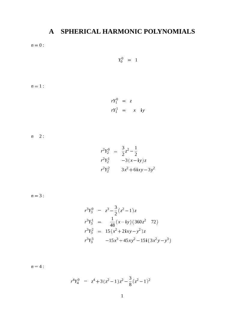
The spherical harmonicsYmn are ordered so that with increasing number the degree increases (see
Appendix A for a listing of the harmonics as trivariate polynomials). This system is then solved
for thecl . A different set ofcl is required for each pointp0 and the stencil of points around it. For
the shallow water equations, the stencil coefficients are calculated for each of the linear operators,
L(U) = ∂U∂x ; ∂U
∂y ; ∂U∂z , and the Laplacian,∆U . This approach is general and is applicable to any
distribution of points on the sphere.
The sense of the approximation in Equation 37 is as a least squares problem for Equation 38.
The problem can be stated in matrix form: findc which minimizes
kHcdk22 (39)
whereH is a N np matrix of spherical harmonics evaluated at points of the stencil andd is
the vector of the exact linear operator applied to the harmonics evaluated at the point. The least
squares problem can be solved elegantly using the singular value decomposition (SVD) [7]. Let
H = USVT be the SVD. The matrixS=diag(σ1;σ2; : : : ;σnp) is the matrix of singular values in
descending order. The solution to the least squares problem is
c= VS1UTd (40)
The choice ofN andnp determine the formal accuracy and smoothness of the derivative ap-
proximations. In general, we choosenp points that are nearly symmetric about the pointp0. The
number of points used in the stencil will determine the efficiency of the method because evaluation
of the derivatives requires a combination of values from these neighboring points. For the icosa-
hedral grid, each point has five or six immediate neighbors (np= 7) (See Fig. 1). If the immediate
neighbors of each of these points are included in the stencil, thennp= 19.
A smoothing parameter that can be introduced in the approximation is the truncation level in the
SVD solution. The diagonal matrix of singular values,S, can be used to smooth the least squares
9

q Grid Points Triangles hmin(km) hmax(km) have(km) hmin=hmax
- 12 20 6699.0 6699.0 6699.0 1.00000 42 80 3482.0 3938.0 3710.0 0.88431 162 320 1613.0 2070.0 1901.0 0.77922 642 1280 761.1 1049.0 956.2 0.72553 2562 5120 368.4 526.3 478.8 0.70014 10242 20480 181.2 263.4 239.5 0.6878
Table 1: Geometric information for icosahedral grids.
solution when the system is underdetermined. By truncating the singular values that are smaller
than some variable tolerance, a solution forc is obtained which supresses unwanted oscillations.
This truncation gives a solution regardless of the underdetermined or overdetermined nature of the
least squares problem. We have found it advantageous to use the same truncation at all points. For
np= 7, we truncate at six because the primary points of the icosahedron have only five neighbors.
The coefficients are unique at these points and of minimum norm at the other points.
4.1 NUMERICAL RESULTS FOR THE GRADIENT APPROXIMATION
The basic icosahedral mesh consists of 20 spherical triangles on 12 grid points. Each of the twelve
points of the mesh is connected to five neighboring points. The refinements of this mesh are
subdivisions of the twenty base triangles. By placing three points on each edge of each large
triangle, and dividing each triangle into three subtriangles, theq= 0 mesh is obtained by projection
of the points (and edges) onto the surface of the sphere. Halving this mesh results in theq= 1 mesh
and halving again gives theq= 2 mesh. The number of points in the mesh is given by the formula,
GP(q) = 5(22q+3)+2 (41)
Table 1 gives geometric information about the different icosahedral meshes.
To check the accuracy of the gradient approximations, a test function exhibiting all modes was
used:
φ(λ;θ) = a(expx+expy+expz): (42)
The errors in the following tables are derived from the Cartesian approximation of the gradient of
this function. The exact values of the function at the vertices of the icosahedral mesh are computed
and used in the difference formulas to approximate the Cartesian derivatives. The Cartesian gra-
10

dient is then transformed to spherical coordinates and compared with the exact gradient ofφ. The
error reported is thel2-error over the points of the icosahedral mesh.
The choice ofN, the number of spherical harmonics andnp, the number of points in the stencil,
determines the formal accuracy of the method. IfN = 9, then spherical harmonics of second order
are used. IfN = 16, then third order harmonics are included. ForN = 25, fourth order harmonics
are included. On an icosahedral grid each point is in a cluster of six or seven. Adding neighbors of
these points with some symmetry leads to either thirteen or nineteen point clusters. These clusters
define the stencil of the discrete operator (see Figure 1 ).
18
0
1
2
4
5 6
3
7
8
9
10 12
11
13
1415
16
17
Fig. 1: Approximation stencil for a regular point of an icosahedral grid.
Plotting the error in Figure 2 with a log-log scale shows the second order (or greater) conver-
gence of the approximation as the mesh spacing is decreased. Though the gradient approximations
appear to be accurate for higher order spherical harmonics, we will restrict attention in this paper
to the quadratic case usingN = 9 andnp= 7.
5 TEST CASES
A set of test cases for the shallow water equations on a sphere are detailed in [24]. These cases
provide a rigorous test for methods as well as allowing for comparison between methods.
11

100.0 1000.0 10000.0hmax (km)
1.0e-08
1.0e-06
1.0e-04
1.0e-02
1.0e+00
l2 er
ror
np=7, N=9np=7, N=16np=19, N=16np=19, N=25
Fig. 2: Convergence of the Gradient Approximations.
5.1 ADVECTION TEST
Test Case 1 is a pure advection problem in which a cosine bell is blown around the sphere under
a constant velocity field. Figure 3 shows the relative RMS error in the geopotential field as a
function of time for a variety of grids. The operators are approximated with quadratic spherical
harmonics and use only nearest neighbors. No diffusion was used for this case. The timestep was
1200 seconds for meshesq= 1;2;3 and 600 seconds for theq= 4 mesh. As can be seen from
Figure 3, the error decreases with mesh refinement. A contour plot of the error (not shown) reveals
a significant wake behind the cosine bell as a result of the centered spatial approximation. Thus,
while convergent, the method has deficiencies as an advection scheme.
5.2 STEADY, ZONAL FLOW TEST
Test Case 2 is a steady, non-linear zonal flow rotated through an angle,α = π4. It tests the ability
of the code to maintain a steady state solution independent of the grid orientation and gives a good
idea of the accuracy of the methods. The velocity and geopotential for this test case are exactly
representable with the spherical harmonics of second order. Hence, the local spherical harmonic
approximations for the derivative operators are able to capture the steady state solution extremely
well. Figures 4 and 5 show the error, as a function of time, in the velocity (using the relative
12

0.0 100.0 200.0 300.0Time (hours)
0.00
0.02
0.04
0.06
0.08
rela
tive
RMS
erro
r (h)
Fig. 3: Relative RMS Error in height; Test Case 1;q= 1;2;3;4.
RMS error with the exact steady solution) and the RMS error in the height field, respectively. The
q= 2;3 integrations used a time step of 1200 seconds for the 5 day (120 hour) simulations while
theq= 4 mesh used a 600 second timestep. For the standard formulation, two diffusion terms were
added. The momentum equation was modified with a diffusion operator,εV∆V, whereεV = 8000.
Similarly, the height equation was modified with a diffusion coefficient ofεh = 20000. For the
rotational formulation, no diffusion was added.
The rotational form gives somewhat better results with no diffusion added. Figures 6 and 7
show the velocity error and the height error for the rotational form of the Cartesian equations also
using the quadratic approximation on six or seven neighbors. The error growth for this form is
more controlled.
A contour plot of the absolute geopotential error is given in Figure 8. The error is measured at
five days. Clearly evident are the base points of the icosahedral grid where the difference stencil
involves six rather than seven points.
The error is held to a small level. However, the error shown in Figure 8 exhibits a curious wave
#5 mode. Other methods based on latitude-longitude grids do not exhibit a systematic error in wave
#5. Since there are five icosahedral points around the earth at a given latitude, this raises questions
about the influence of the truncation error on the computed solution. What is the expected growth
13

0.0 50.0 100.0 150.0Time (hours)
1.0e-05
1.0e-04
1.0e-03
1.0e-02
1.0e-01
1.0e+00
relat
ive R
MS
erro
r (V)
Fig. 4: Relative RMS Error in velocity; Test Case 2;q= 2;3;4; Standard Form.
0.0 50.0 100.0 150.0Time (hours)
1.0e-08
1.0e-06
1.0e-04
1.0e-02
1.0e+00
relat
ive R
MS
erro
r (h)
Fig. 5: Relative RMS Error in height; Test Case 2;q= 2;3;4; Standard Form.
14

0.0 50.0 100.0 150.0Time (hours)
1.0e-05
1.0e-04
1.0e-03
1.0e-02
relat
ive R
MS
erro
r (V)
Fig. 6: Relative RMS Error in Velocity; Test Case 2;q= 2;3;4; Rotational Form.
0.0 50.0 100.0 150.0Time (hours)
1.0e-08
1.0e-07
1.0e-06
1.0e-05
1.0e-04
1.0e-03
1.0e-02
reala
tive
RMS
erro
r (h)
Fig. 7: Relative RMS Error in Height; Test Case 2;q= 2;3;4; Rotational Form.
15

Fig. 8: Error in Geopotential at 5 days; Test Case 2;q= 4; Rotational Form.
of this error in the nonlinear model due to a perturbation of the initial conditions? To explore this
question the computed geopotential from the Cartesian model after one day was used as an initial
condition in a spectral shallow water equation model, STSWM [4]. The spectral code was run at
T42 resolution. After day five, the STSWM Fourier spectrum at a given latitude is compared to the
spectrum of the Cartesian models solution for each day (Figure 9). The Fourier mode amplitude
is the square of the modulus of the complex Fourier coefficient of the geopotential. The Fourier
coefficients were sampled at the latitude of the T42 spectral model nearest 26.6 degrees, which is
the location of one set of icosahedral points and the latitude of highest error in the geopotential.
The solution spectrums do not match but show the same features. The Cartesian solution has
modes 5, 10, and 15 arising from the icosahedral points. These modes appear to grow over time
in the Cartesian model, but no more so than the other modes. The perturbed spectral solution
maintains the strong mode #5 components at Day 5 with some redistribution of the other modes.
The diffusion characteristics of the two methods seem evident. The continued growth of error in
the Cartesian model might be attributed to the truncation errors injected in the solution at each
timestep. The growth is not a nonlinear mode interaction since the perturbed spectral model shows
a preservation of the mode 5 amplitude.
When the Cartesian solution is used as an initial condition in the spectral model, the errors are
16

0.0 5.0 10.0 15.0Fourier Wave Number (m)
1.0e-10
1.0e-05
1.0e+00
1.0e+05
1.0e+10
Wav
e Am
plitu
de
Cartesian t = 0 dayCartesian t = 1 dayCartesian t = 2 daysCartesian t = 3 daysCartesian t = 4 daysCartesian t = 5 daysPerturbed T42 at 5 days
Fig. 9: Comparison of geopotential Fourier spectrum for Case 2;q= 3; Rotational Form.
advected. As these errors (associated with different wave numbers) move around the globe, they
sometimes cancel to produce smaller errors and other times superimpose to create larger errors.
Figure 10 shows the error in the perturbed spectral solution for two different days in the northern
hemisphere. The error on day 4 is considerably more dispersed and smaller than the error on Day 3
or Day 5, indicating a harmonic of the motion. The Cartesian model and the Heikes-Randall [5, 6]
model both show eight peaks of error over the five day period. Once an error is present, it tends
to remain over time, but each model exhibits different numerical diffusion. The Cartesian model
shows a much smoother error than the spectral, indicating that it is more diffusive than the spectral
model. The error profile of the Hiekes-Randall model ([6], Figure 9) also shows less diffusion than
the Cartesian model. It should be reiterated that no diffusion has been explicitly added to any of
these simulations for Case 2.
5.3 NON-ANALYTIC, STEADY, ZONAL FLOW TEST
Test Case 3 is a steady, non-linear zonal flow rotated through some angleα = π3. It is similar to
Test Case 2, however, it contains compactly supported profiles not exactly representable by the
spherical harmonics. The local spherical harmonic approximations for the derivative operators
are able to capture the steady state solution but not as well as in Test Case 2. Figures 11 and 12
17

Fig. 10: Test Case 2, Perturbed Spectral Geopotential Error (a) at Day 4, (b) at Day 5.
show the error, as a function of time, in the velocity (using the relative RMS error with the exact
steady solution) and the RMS error in the height field, respectively. Since the model includes no
damping the error builds over time and then grows exponentially. Theq= 2;3 integrations used a
time step of 1200 seconds for the 5-day (120 hour) simulations while theq= 4 mesh used a 600
second timestep. For this case, no explicit diffusion was added to either the momentum or height
equations.
The rotational form error results for Case 3 are given in Figures 13 and 14. A contour plot of
the absolute geopotential error is given in Figure 15. The error is measured at Day 5.
5.4 FORCED NONLINEAR SYSTEM WITH A TRANSLATING LOW
Test Case 4 is a time-dependent, non-linear forced flow with an exact solution. It tests the perfor-
mance of the scheme in an unsteady, dynamic simulation. The flow is a translating low pressure
center superimposed on a jet stream symmetrical about the equator. The field is similar to a mid-
level tropospheric flow with a short-wave trough embedded in a westerly jet. As the simulation
progresses, the low translates eastward maintaining, its original shape.
Figures 16 and 17 show the error, as a function of time, in the velocity (using the relative RMS
error with the exact solution) and the RMS error in the height field, respectively. The model in
rotational form includes no damping. Theq= 2;3 integrations used a time step of 1200 seconds
18

0.0 50.0 100.0 150.0Time (hours)
1.0e-04
1.0e-03
1.0e-02
1.0e-01
1.0e+00
relat
ive R
MS
erro
r (V)
Fig. 11: Relative RMS Error in Velocity; Test Case 3;q= 2;3;4; Standard Form.
0.0 50.0 100.0 150.0Time (hours)
1.0e-06
1.0e-05
1.0e-04
1.0e-03
1.0e-02
1.0e-01
1.0e+00
1.0e+01
1.0e+02
relat
ive R
MS
erro
r (h)
Fig. 12: Relative RMS Error in Height; Test Case 3;q= 2;3;4; Standard Form.
19

0.0 50.0 100.0 150.0Time (hours)
1.0e-04
1.0e-03
1.0e-02
1.0e-01
1.0e+00
relat
ive R
MS
erro
r (V)
Fig. 13: Relative RMS Error in Velocity; Test Case 3;q= 2;3;4; Rotational Form.
0.0 50.0 100.0 150.0Time (hours)
1.0e-06
1.0e-05
1.0e-04
1.0e-03
1.0e-02
1.0e-01
relat
ive R
MS
erro
r (h)
Fig. 14: Relative RMS Error in Height; Test Case 3;q= 2;3;4; Rotational Form.
20

Fig. 15: Error in Geopotential at 5 days; Test Case 3;q= 4; Rotational Form.
for the 5 day (120 hour) simulations while theq = 4 mesh used a 600 second timestep. The
convergence of the Cartesian method is again exhibited as the mesh is refined.
5.5 ZONAL FLOW OVER AN ISOLATED MOUNTAIN
This Test Case is the only one with orography. A 5400 meter high mountain is given through the
surface height function,hs. No analytical solution is known for this case so the usefulness of the
case is in diagnosing the conservation properties of the numerical scheme. The simulation used a
diffusion coefficient ofεV = 5:0105 with a timestep of 600 seconds for theq= 4 mesh.
The following conserved quantities are presented as functions of time: mass, total energy, and
potential enstrophy. The relative error of the conserved quantity is computed as a normalized inte-
gral of the quantity; the normalization is with respect to the integral of the initial value (see [24]).
The vorticity is presented as an integral without normalization in Figure 18. The conservation
properties of the Cartesian method are much better than expected, considering that the difference
formula used to approximate the conservation of mass is not in flux form and are not guaranteed to
preserve the global mass. The excellent conservation of enstrophy and vorticity are also a surprise.
As normalized integrals it is not evident from Figure 18 that the integral of enstrophy maintains a
value near machine zero ( 1013 ) throughout the simulation. A contour plot of the geopotential
21

0.0 50.0 100.0 150.0Time (hours)
0.00
0.01
0.10
1.00
relat
ive R
MS
erro
r (V)
Fig. 16: Relative RMS Error in Velocity; Test Case 4;q= 2;3;4; Rotational Form.
0.0 50.0 100.0 150.0Time (hours)
0.00
0.01
0.10
1.00
relat
ive R
MS
erro
r (h)
Fig. 17: Relative RMS Error in Height; Test Case 4;q= 2;3;4; Rotational Form.
22

h at Day 15 is given in Figure 19.
0.0 100.0 200.0 300.0 400.0Time (hours)
1.0e-15
1.0e-10
1.0e-05
1.0e+00
Cons
erve
d Qu
anta
ties
nI(mass)nI(energy)nI(enstrophy)I(vorticity)
Fig. 18: Conserved integral quantities; Test Case 5;q= 4; Rotational Form.
5.6 ROSSBY-HAURWITZ WAVE
This classic standard test case [10] does not have an analytic solution for the nonlinear shallow
water equations. The initial conditions are zonal wave #4. The solution at 0, 7, and 14 days
continues to show the strong influence of the initial conditions. A diffusion coefficient ofεV =
1 105 was used for these calculations. Interestingly, this is close to the value of the diffusion
coefficient used by Richardson [11] and also by Williamson [22].
The rotational form is semi-conservative of energy. Figure 20 shows the conserved quantities of
mass, energy, and enstrophy as normalized integrals and the conserved integral of vorticity through
the simulation. A contour plot of the geopotential after 14 simulated days is given in Figure 21.
Departure of the solution from the initial wave #4 is of interest. To examine the structure of
the solution and whether a mode 5 influence is unduly impacting the Cartesian computation, the
experiment using the spectral shallow water code (described in Test Case 2) was repeated. The
Cartesian model geopotential output at Day 1 was used as an initial condition in a spectral shallow
water equation model, STSWM [4]. For reference, the Cartesian solution used for input to the
spectral model is plotted in Figure 22. After 5 days, the STSWM Fourier spectrum was compared
23

Fig. 19: Geopotential at 15 days; Test Case 5;q= 4; Rotational Form.
0.0 100.0 200.0 300.0 400.0Time (hours)
1.0e-20
1.0e-15
1.0e-10
1.0e-05
1.0e+00
Cons
erve
d Qu
antiti
es
nI(mass)nI(energy)ni(enstrophy)I(vorticity)
Fig. 20: Conserved integral quantities; Test Case 6;q= 4; Rotational Form.
24

Fig. 21: Geopotential at 14 days; Test Case 6;q= 4; Rotational Form.
to the spectrum of the Cartesian model solution at the Gaussian latitude nearest 50 degrees north
in Figure 23.
The spectral analysis shows that the growth of low modes in the Cartesian model is similar
to the growth in the spectral model. The low modes grow somewhat but are still three orders
of magnitude less than wave #4. Wave #1-#3 appear stable. Wave #5-#7 grow somewhat over
the five days. In particular, the wave #5 growth is only somewhat larger in the Cartesian model
than in the spectral model. This indicates that the solution is exhibiting an interaction between
modes in response to the perturbed initial conditions. The Cartesian method also shows a small
compounding of truncation errors due to the icosahedral grid points in wave #5. The distribution
of spectral coefficients has more to do with the way energy cascades in the two models. This, in
turn, is related to the diffusion of energy inherent in the models.
The solutions of the perturbed spectral model and the Cartesian model differ only slightly by
the fifth day of the simulation. As seen in Figure 24, the Cartesian method exhibits a smoother
solution due to the added diffusion. The asymmetry that develops in the perturbed spectral model
by Day 14 is not evident, but the high latitude departure from wave #4 is evident. This can be
associated with the growth and interaction of the lower wave numbers. The wave 4 interacts with
the wave 5 in the perturbation to produce a response in wave #1 and wave #9. These modes interact
25

Fig. 22: Cartesian Geopotential at Day 1.
0.0 5.0 10.0 15.0Fourier Wave Number (m)
1.0e-02
1.0e+00
1.0e+02
1.0e+04
1.0e+06
1.0e+08
Wav
e Am
plitu
de
Cartesian t=0 dayCartesian t=5 daysPerturbed T42 at 5 days
Fig. 23: Comparison of geopotential Fourier spectrum for Case 6;q= 3; Rotational Form.
26

with the entire spectrum.
Fig. 24: Test Case 6, (a) Cartesian Geopotential at Day 5, (b) Perturbed Spectral Geopotential at Day5.
5.7 ANALYZED 500mb INITIAL CONDITIONS
The real data initial conditions differ in smoothness from the previous cases, exhibiting much finer
scale structure and sharper gradients. For non-linear calculations, there will be a much stronger
interaction between modes and more active dispersive phenomena. A diffusion coefficient (the
same as for Test Case 6) controls the build up of energy in the fine scales. A timestep of 300
seconds is used on theq= 4 mesh with 10,242 points.
The first test case using analyzed atmospheric conditions is for 000GMT 21 December 1978.
The spectral non-linear normal mode analysis has been used to filter gravity waves from this data.
The NCAR netCDF file “REF0077.cdf” was used for initial conditions of both geopotential and
velocity at the icosahedral grid points. The strong flow over the north pole has been useful in
diagnosing pole problems for several numerical schemes.
Figures 25 shows the conserved quantities of mass, energy, and enstrophy as normalized in-
tegrals and the conserved integral of vorticity through the simulation. Figures 26 and 27 show a
comparison of the reference solution with the Cartesian solution at one and five days, respectively.
27

0.0 50.0 100.0 150.0Time (hours)
1.0e-10
1.0e-08
1.0e-06
1.0e-04
1.0e-02
1.0e+00
Cons
erve
d Qu
antiti
es
nI(mass)nI(energy)nI(enstrophy)I(vorticity)
Fig. 25: Conserved integral quantities; Test Case 7a;q= 4; Rotational Form.
Fig. 26: Test Case 7a, (a) Reference Solution at Day 1, (b) Cartesian Geopotential at Day 1.
28

Fig. 27: Test Case 7, (a) Reference Solution at 5 Day, (b) Cartesian Geopotential at 5 Day.
The second real data case uses the NCAR file “REF0087.cdf”. The flow develops into a typical
blocking situation from an initial condition of two cut-off lows. Initial conditions are for 0000
GMT 16 January 1979. Figures 28 and 29 show a comparison of the reference solution with the
Cartesian solution at Day 1 and Day 5, respectively.
Figures 30 shows the conserved quantities of mass, energy, and enstrophy as normalized inte-
grals and the conserved integral of vorticity through the simulation.
The third real data case has initial conditions from 0000 GMT 9 January 1979 and uses the N-
CAR file “REF0088.cdf”. Initially it has a strong zonal flow. Figures 31 and 32 show a comparison
of the reference solution with the Cartesian solution at Day 1 and Day 5, respectively.
Figures 33 shows the conserved quantities of mass, energy, enstrophy as normalized integrals
and the conserved integral of vorticity through the simulation.
6 CONCLUSIONS
Numerical methods for shallow water equations on the sphere are faced with three hurdles. First,
the geostrophic wind balance must be maintained accurately. The numerical approximation for the
gradient of the geopotential must balance the Coriolis term well. Since the Coriolis term does not
involve derivatives, the gradient approximation is crucial to achieve a reasonable balance. Second,
29

Fig. 28: Test Case 7b, (a) Reference Solution at Day 1, (b) Cartesian Geopotential at Day 1.
Fig. 29: Test Case 7, (a) Reference Solution at 5 Day, (b) Cartesian Geopotential at 5 Day.
30

0.0 50.0 100.0 150.0Time (hours)
1.0e-10
1.0e-08
1.0e-06
1.0e-04
1.0e-02
1.0e+00
Cons
erve
d Qu
antiti
es
nI(mass)nI(energy)nI(enstrophy)I(vorticity)
Fig. 30: Conserved integral quantities. Test Case 7b,q= 4; Rotational Form.
Fig. 31: Test Case 7c, (a) Reference Solution at Day 1, (b) Cartesian Geopotential at Day 1.
31

Fig. 32: Test Case 7c, (a) Reference Solution at 5 Day, (b) Cartesian Geopotential at 5 Day.
0.0 50.0 100.0 150.0Time (hours)
1.0e-10
1.0e-08
1.0e-06
1.0e-04
1.0e-02
1.0e+00
Cons
erve
d Qu
antiti
es
nI(mass)nI(energy)nI(enstrophy)I(vorticity)
Fig. 33: Conserved integral quantities. Test Case 7c,q= 4; Rotational Form.
32

the pole problem must be addressed. Since the spherical coordinate representation of the velocity
is singular at the poles, derivatives must be approximated with care. The third hurdle is to maintain
stability. As nonlinear equations, the consistency of energy conversion terms from potential to
kinetic energy plays a crucial role.
In our work, the first hurdle has been passed by adopting a co-located velocity and gradient
approximation. The collocation method with accurate approximations for the derivatives gives an
excellent balance of the geostrophic wind terms. The second hurdle is passed because the Cartesian
method is free of the pole problem with continuous velocities at the poles. Finally, the third hurdle
is addressed because the rotational form of the equations in Cartesian form gives reasonably good
energy conservation to maintain stability.
The use of least squares fitting of the quadratic spherical harmonics to a seven point stencil
has given second order convergence for the chosen cases. It has also been pointed out [3] that the
Cartesian method does not require the solution of elliptic equations and has a low operation count
with an easy parallel implementation. The deficiencies of the Cartesian method in comparison with
other icosahedral mesh methods like Hiekes and Randall’s [6], are the lack of exact conservation
of enstrophy and a more diffusive scheme. As an advection scheme the Cartesian method suffers
from the same lack of monotonicity as the spectral method.
Future work will involve the testing of higher order Cartesian discretizations and the extension
to a 3-dimensional baroclinic model.
33

References
[1] C. Canuto, M.Y. Hussaini, A. Quarteroni, and T.A. Zang.Spectral Methods in Fluid Dynam-
cis. Springer-Verlag, Berlin, 1988.
[2] I-Liang Chern. A Control Volume Method on a Icosahedral Grid for Numerical Integration
of the Shallow-water Equations on the Sphere . MCS preprint, Argonne National Laboratory,
Chicago, IL, 1991.
[3] J.B. Drake and M.P. Coddington. A Parallel Performance Study of the Cartesian Method
for Partial Differentail Equations on a Sphere. ORNL Tech Report ORNL/TM–13304, Oak
Ridge National Laboratory, Oak Ridge, TN, 1997.
[4] J.J. Hack and R. Jakob. Description of a Global Shallow Water Model Based on the Spec-
tral Transform Method. NCAR Technical Note NCAR/TN-343+STR, National Center for
Atmospheric Research, Boulder, CO, 1992.
[5] Ross Heikes and David A. Randall. Numerical Integration of the Shallow-Water Equations
on a Twisted Icosahedral Grid. Part I.Mon. Wea. Rev., 123:1862–1880, 1995.
[6] Ross Heikes and David A. Randall. Numerical Integration of the Shallow-Water Equations
on a Twisted Icosahedral Grid. Part II.Mon. Wea. Rev., 123:1881–1887, 1995.
[7] C.L. Lawson and R.J. Hanson.Solving Least Squares Problems. Prentice-Hall, Englewood
Cliffs, NJ, 1974.
[8] B. Machenhauer. The spectral method. InNumerical Methods Used in Atmospheric Models,
volume II of GARP Pub. Ser. No. 17. JOC, chapter 3, pages 121–275. World Meteorological
Organization, Geneva, Switzerland, 1979.
[9] Y. Masuda and H. Ohnishi. An Integration Scheme of the Primitive Equation Model with an
Icosahedral-Hexagonal Grid System and its Application to the Shallow Water Equations. In
Short- and Medium-Range Numerical Weather Prediction, pages 317–326, 1986.
[10] N. A. Phillips. Numerical Integration of the Primitive Equations on the Hemisphere.Mon.
Wea. Rev., 87:333–345, 1959.
34

[11] L.F. Richardson. Atmospheric Diffusion Shown on a Distance Neighbour Graph.Proc. Roy.
Soc. Ser. A, 110:709–737, 1928.
[12] R. Sadourny, A. Arakawa, and Y. Mintz. Integration of the Nondivergent Barotropic Vorticity
Equation with an Icosahedral-Hexagonal Grid for the Sphere.Mon. Wea. Rev., 96:351–356,
1968.
[13] R. Sadourny and P. Morel. A Finite-Difference Approximation of the Primitive Equations for
a Hexagonal Grid on a Plane.Mon. Wea. Rev., 97:439–445, 1969.
[14] I. A. Stegun. Legendre functions. In M. Abramowitz and I. A. Stegun, editors,Handbook of
Mathematical Functions, chapter 8, pages 332–353. Dover Publications, New York, 1972.
[15] P. N. Swarztrauber. The Approximation of Vector Functions and Their Derivatives on the
Sphere.SIAM J. Numer. Anal., 18:191–210, 1981.
[16] P.N. Swarztrauber. Spectral Transform Methods for Solving the Shallow-Water Equations on
the Sphere.Mon. Wea. Rev., 124(4):730–744, 1996.
[17] P.N. Swarztrauber, D.L. Williamson, and J.B. Drake. The Cartesian Method for Solving of
PDE’s in Spherical Geometry.Dyn. Atm. Ocn., 27:679–706, 1997.
[18] A.N. Tikhonov and A.A. Samarskii.Equations of Mathematical Physics. Dover Publications,
New York, 1963.
[19] D. L. Williamson. Integration of the Barotropic Vorticity Equation on a Spherical Geodesic
Grid. Tellus, 20:642–653, 1968.
[20] D. L. Williamson. Integration of the Primitive Barotropic Model Over a Spherical Geodesic
Grid. Mon. Wea. Rev., 98:512–520, 1969.
[21] D. L. Williamson. Numerical Integration of Fluid Flow Over Triangular Grids.Mon. Wea.
Rev., 97:885–895, 1969.
[22] D. L. Williamson. A Comparison of First- and Second-Order Difference Approximations
over a Spherical Geodesic Grid.J. Comp. Phys., 7:301–309, 1971.
35

[23] D. L. Williamson. Numerical Methods Used in Atmospheric Models, chapter 2, pages 51–
120. GARP Pub. Ser. No. 17. JOC, WMO, Geneva, Switzerland, 1979.
[24] D. L. Williamson, J.B. Drake, J.J. Hack, Rudiger Jakob, and P.N. Swarztrauber. A Standard
Test Set for Numerical Approximations to the Shallow Water Equations on the Sphere.J.
Comp. Phys., pages 211–224, 1992.
36
A SPHERICAL HARMONIC POLYNOMIALS
n= 0 :
Y00 = 1
n= 1 :
rY01 = z
rY11 = x i y
n= 2 :
r2Y02 =
32
z212
r2Y12 = 3(x+ i y)z
r2Y22 = 3x2+6i xy3y2
n= 3 :
r3Y03 = z3+
32(z21)z
r3Y13 =
148
(x+ i y)(360z272)
r3Y23 = 15(x2+2i xyy2 )z
r3Y33 = 15x3+45xy215i (3x2yy3)
n= 4 :
r4Y04 = z4+3(z21)z2+
38(z21)2
1

r4Y14 =
1384
(x+ i y)(3840z3+2880(z21)z)
r4Y24 =
1384
(x2+2i xyy2 )(20160z22880)
r4Y34 = 105(x33xy2+ i (3x2yy3))z
r4Y44 = 105x4630x2y2+105y4+105i (4x3y4xy3)
n= 5 :
r5Y05 = z5+5(z21)z3+
158(z21)2z
r5Y15 =
13840
(x+ i y)57600z4+86400(z21)z2+7200(z21)2
r5Y25 =
13840
(x2+2i xyy2 )(403200z3+201600(z21)z)
r5Y35 =
13840
(x33xy2+ i (3x2yy3 ))(1814400z2201600)
r5Y45 = 945(x46x2y2+y4+ I (4x3y4xy3 ))z
r5Y55 = 945x5+9450x3y24725xy4945i (5x4y10x2y3+y5)
n= 6 :
r6Y06 = z6+
152(z21)z4+
458(z21)2z2+
516
(z21)3
r6Y16 =
146080
(x+ i y)
967680z5+2419200(z21)z3+604800(z21)2z
r6Y26 =
146080
(x2+2i xyy2 )9676800z4+9676800(z21)z2+604800(z21)2
r6Y3
6 = 1
46080(x33xy2+ i (3x2yy3))(58060800z3+21772800(z21)z)
r6Y46 =
146080(x46x2y2+y4+ i (4x3y4xy3 ))(239500800z221772800)
r6Y56 = 10395(x510x3y2+5xy4+ i (5x4y10x2y3+y5))z
2

r6Y66 = 10395x6155925x4y2+155925x2y410395y6
+10395i (6x5y20x3y3+6xy5)
3