carbon dynamics and greenhouse gas emissions of standing ...€¦ · carbon dynamics and greenhouse...
TRANSCRIPT

E n e r g y R e s e a r c h a n d De v e l o p m e n t Di v i s i o n
F I N A L P R O J E C T R E P O R T
CARBON DYNAMICS AND GREENHOUSE GAS EMISSIONS OF STANDING DEAD TREES IN CALIFORNIA MIXED CONIFER FORESTS
JUNE 2014 CEC-500 -2016-001
Prepared for: California Energy Commission Prepared by: University of California Berkeley

Prepared by: Primary Authors: John J. Battles Stella J.M. Cousins John E. Sanders University of California Berkeley Department of Environmental Science, Policy, and Management 130 Mulford Hall #3114 Berkeley, CA 94720 Phone: 510-643-2450 Contract Number: 500-10-046 Prepared for: California Energy Commission David Stoms Project Manager
Aleecia Gutierrez Office Manager Energy Generation Research Office
Laurie ten Hope Deputy Director ENERGY RESEARCH AND DEVELOPMENT DIVISION
Robert P. Oglesby
Executive Director
DISCLAIMER This report was prepared as the result of work sponsored by the California Energy Commission. It does not necessarily represent the views of the Energy Commission, its employees or the State of California. The Energy Commission, the State of California, its employees, contractors and subcontractors make no warranty, express or implied, and assume no legal liability for the information in this report; nor does any party represent that the uses of this information will not infringe upon privately owned rights. This report has not been approved or disapproved by the California Energy Commission nor has the California Energy Commission passed upon the accuracy or adequacy of the information in this report.

i
ACKNOWLEDGEMENTS
The authors gratefully acknowledge those who assisted with sample collection and preparation:
Debra Larson, David Soderberg, Eric Olliff, Alexander Javier, Natalie Holt, Clayton Sodergren,
Erika Blomdahl, and Joe Battles. The authors further thank Robert York, Research Director at
Blodgett Forest Research Station, for his generous contributions to site selection efforts and
permission to sample trees. Thanks also to Ken Somers and Pete Zellner for their work safely
choosing and felling trees. Finally, we are grateful to cooperators Adrian Das and Nathan
Stephenson of the United States Geologic Survey - Western Ecological Research Station and
Koren Nydick of the National Park Service for their assistance with sampling and analysis of
the Forest Demography Study plots in Sequoia and Kings Canyon National Parks.

ii
PREFACE
The California Energy Commission Energy Research and Development Division supports
public interest energy research and development that will help improve the quality of life in
California by bringing environmentally safe, affordable, and reliable energy services and
products to the marketplace.
The Energy Research and Development Division conducts public interest research,
development, and demonstration (RD&D) projects to benefit California.
The Energy Research and Development Division strives to conduct the most promising public
interest energy research by partnering with RD&D entities, including individuals, businesses,
utilities, and public or private research institutions.
Energy Research and Development Division funding efforts are focused on the following
RD&D program areas:
Buildings End-Use Energy Efficiency
Energy Innovations Small Grants
Energy-Related Environmental Research
Energy Systems Integration
Environmentally Preferred Advanced Generation
Industrial/Agricultural/Water End-Use Energy Efficiency
Renewable Energy Technologies
Transportation
Carbon Dynamics and Greenhouse Gas Emissions of Standing Dead Trees in California Mixed Conifer
Forests is the final report for the Carbon Dynamics And Greenhouse Gas Emissions From Standing
Dead Trees In California Forests project (grant number 500‐10‐046) conducted by the University of
California Berkeley. The information from this project contributes to the Energy Research and
Development Division’s Energy-Related Environmental Research Program.
For more information about the Energy Research and Development Division, please visit the
Energy Commission’s website at www.energy.ca.gov/research/ or contact the Energy
Commission at 916-327-1551.

iii
ABSTRACT
Increasing climatic stress, outbreaks of pests, and chronic air pollution have contributed to a
global pattern of escalating forest mortality. These trends result in an unprecedented abundance
of standing dead trees, with immediate implications for the dynamics of carbon sequestration
and emissions by forests. Increases in standing dead trees also represent a transformation of
basic ecosystem structures and functions. This study contributed to calculating accurate forest
greenhouse gas budgets by characterizing the decay and demographic processes of standing
dead trees and incorporating these characteristics into regional inventories and projections of
forest carbon storage. The authors used dimensional analysis to describe dead tree conditions
and field studies to quantify the fall rate of standing dead trees. These results were combined
with a new approach for a remotely sensed greenhouse gas assessment for California's
forestlands to estimate carbon storage and emissions from trees. To project potential losses due
to forest disturbance, the researchers simulated a bark beetle irruption and examined the impact
on greenhouse gas budgets over ten years. The investigation found that methods that do not
incorporate carbon density losses overestimate the carbon storage of standing dead trees in
California mixed conifer forests by 18.8 percent. More than 90 percent of standing dead trees
were expected to fall within ten years of their death, with pine species falling at rates slightly
faster than firs. Results from this project directly support the California Air Resources Board to
implement AB32. In addition, these results suggest that the forest sector sequesters less carbon
than previously estimated in standing dead trees.
Keywords: biomass, carbon, decay, demography, forest inventory, emissions, fall rate,
greenhouse gas inventory, mixed conifer, Sierra Nevada, snag, standing dead trees
Please use the following citation for this report:
Battles, John J., Cousins, Stella J. M., and Sanders, John E. (University of California Berkeley).
2015. Carbon Dynamics and Greenhouse Gas Emissions of Standing Dead Trees In
California Mixed Conifer Forests. California Energy Commission. Publication number:
CEC-500-2016-001.

iv
TABLE OF CONTENTS
Acknowledgements ................................................................................................................................... i
PREFACE ................................................................................................................................................... ii
ABSTRACT .............................................................................................................................................. iii
TABLE OF CONTENTS ......................................................................................................................... iv
LIST OF FIGURES ................................................................................................................................. vii
LIST OF TABLES ................................................................................................................................... vii
EXECUTIVE SUMMARY ........................................................................................................................ 1
Introduction ................................................................................................................................................ 1
Project Purpose ........................................................................................................................................... 1
Project Process and Results ....................................................................................................................... 1
Project Benefits ........................................................................................................................................... 3
CHAPTER 1: Overview: Forest Carbon Inventorying and Monitoring ......................................... 4
1.1 Need for Forest Carbon Inventory and Monitoring ........................................................... 4
1.2 IPCC Recommended Protocols ............................................................................................... 4
1.3 Past and Proposed Approaches to Forest GHG Accounting in California .................... 5
1.4 Gaps in Assessment of Standing Dead Tree Carbon ......................................................... 5
1.4.1 Biological Gaps ........................................................................................................................... 5
1.4.2 California Challenge .................................................................................................................. 6
1.4.3 National Challenge .................................................................................................................... 7
1.5 Overview of this Project .......................................................................................................... 8
1.5.1 Measure the Carbon Density in Standing Dead Trees in California Mixed Conifer
Forests ...................................................................................................................................................... 8
1.5.2 Quantify the Fall Rates of Standing Dead Trees in the California Mixed Conifer Forests
...................................................................................................................................................... 8
1.5.3 Enhance Current Methods to Assess Gain-Loss of Carbon from Standing Dead Trees in
California’s Conifer Forests ...................................................................................................................... 8
CHAPTER 2: Carbon Density of Standing Dead Trees in California Conifer Forests .............. 10
2.1 Introduction ............................................................................................................................. 10

v
2.1.1 Background ............................................................................................................................... 10
2.1.2 Problem Statement: Current Approaches for Biomass Estimates in SDT ........................ 11
2.1.3 Carbon Density Study Objectives .......................................................................................... 11
2.2 Methods .................................................................................................................................... 12
2.2.1 Site Descriptions ....................................................................................................................... 12
2.2.2 Sampling Regime ..................................................................................................................... 13
2.2.3 Allometric Scaling .................................................................................................................... 17
2.2.4 Whole Tree Biomass, Density Reduction Factors and Carbon Density ........................... 18
2.2.5 Analysis ..................................................................................................................................... 18
2.3 Results ....................................................................................................................................... 18
2.3.1 Volume and Wood Density Loss ........................................................................................... 18
2.3.2 Carbon Concentration and Total Carbon Biomass as a Function of Species and Decay
Class .................................................................................................................................................... 20
2.3.3 Bark Decay Patterns and Effect on Whole Tree Biomass ................................................... 21
2.3.4 Net Change in Biomass and Carbon Stored ......................................................................... 22
2.4 Discussion ................................................................................................................................ 23
2.4.1 Patterns in Biomass Loss ......................................................................................................... 23
2.4.2 Attribution of Carbon Loss: Volume Loss vs. Decay .......................................................... 24
2.4.3 Evaluation of Uncertainty ....................................................................................................... 24
CHAPTER 3: Fall Rates of Standing Dead Trees in California Mixed Conifer Forests ............ 27
3.1 Introduction ............................................................................................................................. 27
3.2 Methods .................................................................................................................................... 28
3.2.1 Site Descriptions ....................................................................................................................... 28
3.2.2 Standing Dead Inventories ..................................................................................................... 29
3.2.3 Standing Dead Tree Fall Rate Analysis ................................................................................. 31
3.2.4 Incorporating Existing SDT Information .............................................................................. 32
3.3 Results ....................................................................................................................................... 32
3.3.1 Shape and Magnitude of the Fall Rate Curve ...................................................................... 32
3.3.2 Survival Rates of Standing Dead Trees by Species and Size Class ................................... 33

vi
3.3.3 A Comparison of SDT Fall Rates for California Mixed Conifer Tree Species ................. 41
3.4 Discussion ................................................................................................................................ 42
CHAPTER 4: Improving California’s Greenhouse Gas Accounting for Forest and Rangelands:
Tracking Gains and Losses in the Standing Tree Carbon Pool ..................................................... 44
4.1 Introduction ............................................................................................................................. 44
4.1.1 Background ............................................................................................................................... 44
4.1.2 Problem Statement ................................................................................................................... 46
4.2 Methods .................................................................................................................................... 46
4.2.1 Developing GHG Accounting Approach ............................................................................. 46
4.2.2 Estimating Standing Dead Tree Carbon ............................................................................... 47
4.2.3 Incorporation of Revised Estimate (Chapter 2) of Standing Dead Tree Carbon Pools .. 49
4.2.4 Analytical Framework for Projecting Carbon Dynamics of Dead Trees .......................... 50
4.3 Results ....................................................................................................................................... 50
4.3.1 Performance of LANDFIRE to Detect Changes in Standing Dead Tree Biomass ........... 50
4.3.2 Performance of FIA in Estimating Standing Dead Tree Carbon ....................................... 51
4.3.3 Impact of Improvements on Carbon Stocks and GHG Estimates ..................................... 53
4.3.4 Five and Ten-Year Projections of SDT Carbon Storage ...................................................... 53
4.4 Discussion ................................................................................................................................ 54
4.4.1 Implications of Dead Tree Assessment Strategies to GHG Accounting .......................... 54
4.4.2 Implications of Dead Tree Assessment to GHG Accounting Under Scenarios of
Increasing Tree Mortality ........................................................................................................................ 55
CHAPTER 5: Conclusions ..................................................................................................................... 56
5.1 Contributions of Project to Carbon Science and Ecosystem Ecology ........................... 56
5.2 Impact of Enhancements on Current GHG Monitoring in California ......................... 56
5.3 Future Directions and Next Steps ........................................................................................ 57
5.3.1 Rationale for Efforts to Enhance Understanding of Dead Tree Carbon Ecology ............ 57
5.3.2 Limitations of LANDFIRE ...................................................................................................... 58
5.3.3 Immediate Next Steps ............................................................................................................. 58
5.3.4 Promise of LandTrendr: A Novel Technology Designed to Detect Forest Disturbance 58
vii
5.4 Benefits to California ....................................................................................................................... 59
GLOSSARY .............................................................................................................................................. 60
REFERENCES .......................................................................................................................................... 62
LIST OF FIGURES
Figure 1: Current standing dead and dying trees, Sequoia National Park ........................................ 6
Figure 2: Forest Inventory and Analysis Decay Class Framework ................................................... 14
Figure 3: Technique for Dimensional Analysis; Sampling and Measuring Volume of Decayed
Wood .......................................................................................................................................................... 16
Figure 4. Density (g cm-3) of Decay Classes 1-5 by Tree Taxonomic Group ................................... 20
Figure 5: Carbon Concentration of Decay Classes 1-5 by Tree Taxonomic Group......................... 21
Figure 6: Standing Dead Tree Carbon Concentration, Density (DRF), and Net Carbon Density
Relative to Live Trees for Each Decay Class ........................................................................................ 23
Figure 7: Standing Dead Tree Fall Rate Curves for Two Longitudinal Studies in California ....... 35
Figure 8: Standing Dead Tree Fall Rate Curves for Three Common Species in Mixed Conifer
Forests (white fir, ponderosa pine, sugar pine) ................................................................................... 36
Figure 9. Standing dead tree fall rate curves for incense cedar, Douglas-fir, and black oak trees
at BFRS ....................................................................................................................................................... 37
Figure 10: Standing Dead Tree Fall Rate Curves for White Fir, Ponderosa Pine, and Sugar Pine
Trees at SEKI ............................................................................................................................................. 38
Figure 12: Standing Dead Tree Fall Rate Curves for Red Fir and Jeffrey Pine Trees at SEKI ....... 40
Figure 13: Distribution of Standing Dead Tree Annual Fall Rates for Pine Species in the Montane
Forests of the Western United States (n = 31) ....................................................................................... 42
Figure 14: Standing Dead Tree Aboveground Biomass in the Mixed Conifer Forests as a
Function of Canopy Cover Class and Height Class for the California Mixed Conifer Forest ...... 51
Figure 15: Relationship Between Aboveground Standing Dead Tree Carbon Density and
Aboveground Live Tree Carbon Density for the 766 FIA Plots ........................................................ 52
Figure 16: Magnitude of the Overestimate in Aboveground Standing Dead Tree Carbon Density
as a Function of Canopy Cover and Height Class for the California Mixed Conifer Forest ......... 52
Figure 17: Decline in the Standing Dead Tree Carbon Pool Following a Simulated Beetle-Attack
on Pine Trees in the California Mixed Conifer Forest ........................................................................ 54

viii
LIST OF TABLES
Table 1: Standing Dead Tree Characteristics by Species, Decay Class, and Diameter Class ........ 19
Table 2: Mean Combined Standing Dead wood and Bark Density and Dead:Live Density Ratio
for Each Decay Class................................................................................................................................ 19
Table 3: Mean Combined Standing Dead Wood and Bark Carbon Concentration and Dead:Live
Carbon Concentration Ratio for Each Decay Class ............................................................................. 21
Table 4: Wood Characteristics: Mean Standing Dead: Live Density Ratio and Mean Carbon
Concentration for Each Decay Class ..................................................................................................... 22
Table 5: Bark Characteristics: Mean Standing Dead:Live Density Ratio and Mean Carbon
Concentration for Each Decay Class ..................................................................................................... 22
Table 6: After Density Losses and Carbon Gains, Mean Dead:Live Net Carbon Ratio of
Combined Wood and Bark for Each Decay Class ............................................................................... 23
Table 7: Properties of Standing Dead Trees (wood and bark combined) for All Species and
Decay Classes Sampled ........................................................................................................................... 25
Table 8: Standing Dead Wood Properties and Bark Properties for All Species and Decay Classes
Sampled ..................................................................................................................................................... 26
Table 9: Description of Sites/Data from California Conifer Forests Used in This Report .............. 29
Table 10: Standing Dead Tree Fall Rates for Blodgett Forest Research Station ............................... 30
Table 11: Standing Dead Tree Fall Rates for Sequoia-Kings Canyon National Parks .................... 31
Table 12: Standing Dead Tree Fall Rates for Sequoia-Kings Canyon National Parks .................... 34
Table 13: Comparison of Standing Dead Tree Fall Rates for Pine and True Fir Species in Four
California Forests ..................................................................................................................................... 41
Table 14: Summary of Major Remote Sensing Technologies Used for Assessing Carbon Stocks 45

1
EXECUTIVE SUMMARY
Introduction
About half of a tree’s mass is made of carbon. As trees grow, they take in carbon dioxide from
the air and convert it into leaves, bark, stem, and roots. As they die and decay, that carbon is
released back into the atmosphere as carbon dioxide, a greenhouse gas. Tree death and decline
are natural ecosystem processes, but forest mortality rates have recently accelerated and are
continuing to climb well above historic levels. Both in California’s forests and worldwide,
increasing climatic stress, outbreaks of pests, and chronic air pollution have contributed to
catastrophic forest die-offs. Dead trees are now a more important component of forest stands
than before, and in the future their roles will be further pronounced.
These trends of dying trees have broad implications for the dynamics of forest carbon storage
and greenhouse gas emissions, and therefore for California’s climate strategy. This strategy
relies heavily on healthy forests to remove carbon dioxide emissions from energy,
transportation, and other sectors. With increasing numbers of trees dying, the scales could be
tipped so that forests release more carbon than they absorb. California regulators need accurate
greenhouse gas accounting to predict the capacity of California forests to store and sequester
carbon. However, there are gaps in knowledge about some of the details of these processes. For
instance, it is unknown how fast different species of trees decompose. Furthermore, there is no
good estimate of the greenhouse gas emissions due to landscape-scale disturbance and resulting
mortality, such as a widespread beetle kill. This important challenge must be addressed to
inform California’s climate strategy, including the amount of carbon offsets available to energy
utility operators.
Project Purpose
The California Air Resources Board inventories and regulates greenhouse gas from forests and
rangelands, including those from dead trees, through the Global Warming Solutions Act,
Assembly Bill 32. Meaningful, accurate greenhouse gas budgets are necessary to predict the
capacity of California forests to store and sequester carbon; this directly relates to decisions
about the amount of carbon offsets that energy utility operators can purchase or the amount of
greenhouse gas emissions that they will have to reduce by other means. To further refine forest
carbon accounting methods, this project:
Measured the carbon density of standing dead trees in California’s mixed conifer forests,
Quantified how long it takes for standing dead trees in California’s mixed conifer forests
to fall to the ground, and
Used this data to improve estimates of carbon and greenhouse gas emissions from
standing dead trees, evaluate remote sensing products that inform these estimates, and
assess the expected emissions from a pest-driven forest disturbance.
Project Process and Results
This investigation of the carbon dynamics and greenhouse gas emissions of standing dead trees
focused on California’s mixed conifer forests, the most extensive forest type in the state. Mixed

2
conifer forests dominate the Sierra Nevada range and occupy 5.3 percent of California’s total
land area (21,500 km2). Research sites included Blodgett Forest Research Station and the US
Geological Survey Forest Demography plot network in Sequoia, Kings Canyon, and Yosemite
National Parks. The study also incorporated standing dead tree data from previous studies in
the region. The authors intentionally used the same decay classification used by the US Forest
Service’s Forest Inventory and Analysis program, since many large-scale greenhouse gas
assessments rely on it. This classification divides tree decay into five stages.
The study characterized the density, carbon concentration, and net carbon density of trees from
each of five structural stages of decay. As decay advanced, trees showed both a progressively
lower density and a small increase in carbon concentration. Some variation in these patterns
was evident among different species and sizes. The net result for total standing dead tree
carbon density was also a decline, with carbon density in the most decayed trees only 60
percent that of live trees. This is the first measurement of standing dead tree decay patterns in
mixed conifer species and the first time all five stages of decay have been measured.
The longevity of standing dead trees in mixed conifer and pine forests was also examined. This
information is essential to describe the timing of carbon storage and emissions. For standing
dead trees about 16 inches in diameter, half of them fell within 10.1 years at Sequoia-Kings
Canyon National Parks and 4.7 years at Blodgett Forest Research Station. Firs fell more rapidly
than pines overall. Larger diameter dead trees generally remained standing longer than smaller
ones.
To apply carbon density loss and treefall patterns information, the improved estimates of
standing dead carbon were combined in a new framework for repeatable forest sector
greenhouse gas inventory. The carbon stored in standing dead trees is systematically
overestimated by current methods that do not correct for decay. When estimates correct for
decay, standing dead trees represent 8 percent of aboveground live carbon. Using these same
methods statewide that do not account for changing carbon density results in an 18.8 percent
overestimate of carbon in standing dead trees.
The study evaluated the land use/land cover products and vegetation inventories available to
track biomass changes regarding their capacity to describe and track episodes of forest die-off.
Existing vegetation height, a metric of the remotely sensed LANDFIRE dataset, proved best for
predicting standing dead tree biomass. For forests, standing dead tree biomass significantly
increased with increasing existing vegetation height. The study also projected the carbon
outcomes of a major (35 percent) die-off event in the California mixed conifer forest, as might
occur following a bark beetle irruption. Most of dead trees fell to the forest floor within the first
five years. After ten years, only 8 percent of the original forest carbon remained in standing
trees. In other words, a die-off of this magnitude in the mixed conifer forest would completely
offset 10 years of cumulated tree growth in terms of carbon storage. These results suggest that
the forest sector sequesters less carbon than was previously estimated in standing dead trees
and have implications for calculating the benefit of forest carbon offset projects.

3
Project Benefits
Results from this project directly support the California Air Resources Board and its charge to
implement AB 32 and are essential for resource managers and state policymakers. By improving
the carbon stocks assessment consistent with international guidelines, the project supports
efforts by the California Climate Action Registry to collect data on facility-level and entity-wide
greenhouse gas emissions directed by the 2005 Integrated Energy Policy Report. Specifically,
this research improves the accuracy and completeness of forest carbon accounting and
greenhouse gas budgets for California mixed conifer forests. Adding critical detail on standing
dead tree decay and demographic processes enables informed predictions of the capacity of
California forests to sequester carbon. Implementing these improved estimates as a dynamic
and repeatable forest sector greenhouse gas accounting provides a comprehensive and
ecologically relevant approach for estimating rates of forest carbon emissions. For the first time,
the project delivers original studies of standing dead tree carbon density and develops
information specific to California mixed conifer forests and the full range of decay conditions
quantifying resultant emissions. These initial greenhouse gas emission projections tied to
catastrophic mortality events are a valuable first step toward anticipating the impact of
widespread forest mortality on California forest ecosystems and on the region’s greenhouse gas
budget.
4
CHAPTER 1: Overview: Forest Carbon Inventorying and Monitoring
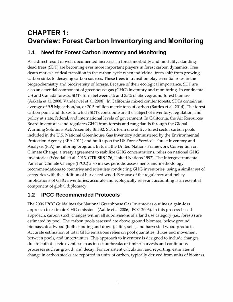
1.1 Need for Forest Carbon Inventory and Monitoring
As a direct result of well-documented increases in forest morbidity and mortality, standing
dead trees (SDT) are becoming ever more important players in forest carbon dynamics. Tree
death marks a critical transition in the carbon cycle when individual trees shift from growing
carbon sinks to decaying carbon sources. These trees in transition play essential roles in the
biogeochemistry and biodiversity of forests. Because of their ecological importance, SDT are
also an essential component of greenhouse gas (GHG) inventory and monitoring. In continental
US and Canada forests, SDTs form between 5% and 35% of aboveground forest biomass
(Aakala et al. 2008, Vanderwel et al. 2008). In California mixed conifer forests, SDTs contain an
average of 9.5 Mg carbon/ha, or 20.5 million metric tons of carbon (Battles et al. 2014). The forest
carbon pools and fluxes to which SDTs contribute are the subject of inventory, regulation, and
policy at state, federal, and international levels of government. In California, the Air Resources
Board inventories and regulates GHG from forests and rangelands through the Global
Warming Solutions Act, Assembly Bill 32. SDTs form one of five forest sector carbon pools
included in the U.S. National Greenhouse Gas Inventory administered by the Environmental
Protection Agency (EPA 2011) and built upon the US Forest Service’s Forest Inventory and
Analysis (FIA) monitoring program. In turn, the United Nations Framework Convention on
Climate Change, a treaty agreement to stabilize GHG concentrations, relies on national GHG
inventories (Woodall et al. 2013, GTR SRS 176, United Nations 1992). The Intergovernmental
Panel on Climate Change (IPCC) also makes periodic assessments and methodology
recommendations to countries and scientists conducting GHG inventories, using a similar set of
categories with the addition of harvested wood. Because of the regulatory and policy
implications of GHG inventories, accurate and ecologically relevant accounting is an essential
component of global diplomacy.
1.2 IPCC Recommended Protocols
The 2006 IPCC Guidelines for National Greenhouse Gas Inventories outlines a gain-loss
approach to estimate GHG emissions (Aalde et al 2006, IPCC 2006). In this process-based
approach, carbon stock changes within all subdivisions of a land use category (i.e., forests) are
estimated by pool. The carbon pools assessed are above ground biomass, below ground
biomass, deadwood (both standing and down), litter, soils, and harvested wood products.
Accurate estimation of total GHG emissions relies on pool quantities, fluxes and movement
between pools, and uncertainties. This approach to inventory is designed to include changes
due to both discrete events such as insect outbreaks or timber harvests and continuous
processes such as growth and decay. For consistent calculation and reporting, estimates of
change in carbon stocks are reported in units of carbon, typically derived from units of biomass.
5
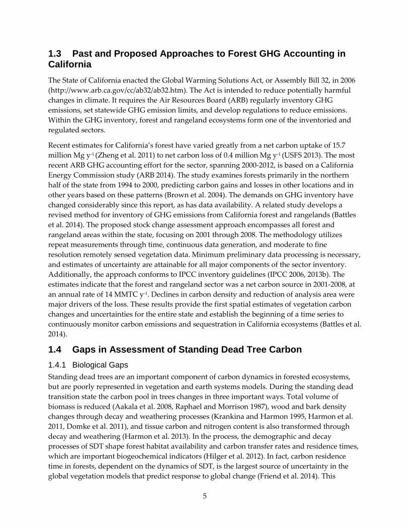
1.3 Past and Proposed Approaches to Forest GHG Accounting in California
The State of California enacted the Global Warming Solutions Act, or Assembly Bill 32, in 2006
(http://www.arb.ca.gov/cc/ab32/ab32.htm). The Act is intended to reduce potentially harmful
changes in climate. It requires the Air Resources Board (ARB) regularly inventory GHG
emissions, set statewide GHG emission limits, and develop regulations to reduce emissions.
Within the GHG inventory, forest and rangeland ecosystems form one of the inventoried and
regulated sectors.
Recent estimates for California’s forest have varied greatly from a net carbon uptake of 15.7
million Mg y-1 (Zheng et al. 2011) to net carbon loss of 0.4 million Mg y-1 (USFS 2013). The most
recent ARB GHG accounting effort for the sector, spanning 2000-2012, is based on a California
Energy Commission study (ARB 2014). The study examines forests primarily in the northern
half of the state from 1994 to 2000, predicting carbon gains and losses in other locations and in
other years based on these patterns (Brown et al. 2004). The demands on GHG inventory have
changed considerably since this report, as has data availability. A related study develops a
revised method for inventory of GHG emissions from California forest and rangelands (Battles
et al. 2014). The proposed stock change assessment approach encompasses all forest and
rangeland areas within the state, focusing on 2001 through 2008. The methodology utilizes
repeat measurements through time, continuous data generation, and moderate to fine
resolution remotely sensed vegetation data. Minimum preliminary data processing is necessary,
and estimates of uncertainty are attainable for all major components of the sector inventory.
Additionally, the approach conforms to IPCC inventory guidelines (IPCC 2006, 2013b). The
estimates indicate that the forest and rangeland sector was a net carbon source in 2001-2008, at
an annual rate of 14 MMTC y-1. Declines in carbon density and reduction of analysis area were
major drivers of the loss. These results provide the first spatial estimates of vegetation carbon
changes and uncertainties for the entire state and establish the beginning of a time series to
continuously monitor carbon emissions and sequestration in California ecosystems (Battles et al.
2014).
1.4 Gaps in Assessment of Standing Dead Tree Carbon
1.4.1 Biological Gaps
Standing dead trees are an important component of carbon dynamics in forested ecosystems,
but are poorly represented in vegetation and earth systems models. During the standing dead
transition state the carbon pool in trees changes in three important ways. Total volume of
biomass is reduced (Aakala et al. 2008, Raphael and Morrison 1987), wood and bark density
changes through decay and weathering processes (Krankina and Harmon 1995, Harmon et al.
2011, Domke et al. 2011), and tissue carbon and nitrogen content is also transformed through
decay and weathering (Harmon et al. 2013). In the process, the demographic and decay
processes of SDT shape forest habitat availability and carbon transfer rates and residence times,
which are important biogeochemical indicators (Hilger et al. 2012). In fact, carbon residence
time in forests, dependent on the dynamics of SDT, is the largest source of uncertainty in the
global vegetation models that predict response to global change (Friend et al. 2014). This

6
transitional period between growth and decomposition on the forest floor needs to be
quantitatively described in order to understand the role of SDT in forest carbon pools and
fluxes, to provide realistic estimates of broader ecosystem processes, and to accurately project
ecosystem greenhouse gas budgets.
1.4.2 California Challenge
In the recent past, SDT formed about 11% of standing trees and 7% of total standing carbon in
California mixed conifer forests (FIADB 2011, Woodall 2012). Within the past decade, however,
California forests have experienced dramatic increases in mortality. Tree mortality in California
is most often attributable to disturbances and environmental conditions including insect
outbreaks, episodic disease, climate, chronic air pollution, and fire. Many of these factors have
intensified and compounded, resulting in a higher proportion of SDT relative to live trees. For
example, the number of standing dead sugar pine trees in Sequoia-Kings Canyon National
Parks (29% of live stems) is four times greater than average for this species in California (7% of
live stems, FIADB 2011). The cause of the increased mortality is thought to be the combined
effects of white pine blister rust, an exotic fungal pathogen, and exposure to high levels of
ozone and nitrogen pollution (Battles et al. 2013). In Sierra Nevada old growth forests, tree
mortality rates across all species have more than doubled in recent decades (van Mantgem and
Stephenson 2007). In 2008-2009, irruptions of bark beetles in California’s coniferous forests
caused a 200-300% increase in pine tree deaths at sites throughout the state. During the same
period, white fir mortality in some locations increased 1000% due to outbreaks of fir engraver
beetle (FIADB 2011). These episodes parallel the unprecedented outbreaks of bark beetles
throughout comparable forests in the western United States and Canada, which have decimated
millions of hectares of forest. Climate change projections and air pollution trends indicate a
future of exacerbated environmental stress both for California’s forests (Battles et al. 2009;
Moser et al. 2009) and forests throughout the western United States (Allen et al. 2010 ). Elevated
tree mortality will drive local increases in GHG emissions and is likely to transform impacted
forest ecosystems from effective sinks to sources of atmospheric C and N greenhouse gas
compounds. However, the demographic attributes of SDT in California forests, including their
decomposition trajectories and standing dead longevity, remain unknown. To improve the
accuracy and ecological relevance of GHG inventory for California’s forest and rangeland
sector, a better understanding of the decay patterns and fall rates of SDT in our forests is
needed.
Figure 1: Current standing dead and dying trees, Sequoia National Park

7
Photo credit: S. Cousins
1.4.3 National Challenge
Forest inventories and carbon accounting efforts in particular have traditionally focused
primarily on growing stock and secondarily on fuels. In these cases, dynamics of SDT are often
roughly estimated or even omitted. Currently, nationwide ground-based inventory of forest
carbon relies on the US Forest Service’s FIA framework. As of the year 2000, the FIA program
has coupled a nationwide approach to inventory with an extensive network of forest plots,
making periodic continental-scale assessments of standing biomass feasible (Heath et al. 2009).
The FIA approach to biomass calculations, known as the Component Ratio Method, sums the
carbon-containing components of each tree. Volume of each component is calculated according
to equations developed for each tree species within each region, with live and dead standing
biomass treated in the same manner (Woodall et al. 2010, Woudenberg et al. 2010). Total bole
biomass relies on a visual approximation of the cull (rotten or unmerchantable) timber volume.
This a major obstacle in accurate estimation of SD biomass, because it fails adjust for the in situ
structural and density losses that characterize SD trees (Heath et al. 2011, Smith et al. 2003).
Additionally, information on the duration any given SDT will remain standing is scarce. The fall
rates of SDT vary with species, region, and many site factors, and are important in shaping the
path and rate of wood decomposition, thus influencing forest emissions (Hilger et al. 2012).

8
A variety of empirically-based decay adjustment factors are in development. These are designed
to lend greater accuracy and relevancy to forest carbon accounting efforts, and focus on both
standing dead and down woody debris (Harmon et al. 2011, Domke et al. 2011). However, none
of the recommended methods have thus far been implemented in regional or national carbon or
GHG estimates. An integrated model that combines the effects of these diverse decay processes
from a carbon dynamics standpoint is needed to estimate net effects on carbon and GHG
budgets.
1.5 Overview of this Project
1.5.1 Measure the Carbon Density in Standing Dead Trees in California Mixed Conifer Forests
In this study, the authors describe the roles of SDT in forest carbon dynamics using three
approaches. First is an assessment of changing carbon density within individual trees (Chapter
2). This investigates the patterns of density and carbon loss within standing dead trees as they
decay. Empirical measurements take a dimensional analysis approach, sampling wood and bark
properties from trees in the decay classes used nationwide by the FIA program. Next, the
degree to which tissue density and carbon concentration varies with tree species, decay class,
and tissue type is determined. These decay patterns are then used to develop density reduction
factors and net carbon reduction factors for each of the major species in California mixed conifer
forests. The resultant SDT biomass and C stock estimates are applied in refining the estimates of
carbon stored in SDT in California’s most common forest type, mixed conifer.
1.5.2 Quantify the Fall Rates of Standing Dead Trees in the California Mixed Conifer Forests
Next, the authors examine longevity of SDT on the landscape (Chapter 3). Two long-term
studies of SDT are used to determine the fall rates of SDT in California mixed conifer forests
and the major drivers of these patterns. For both sites (Blodgett Forest Research Station and
Southern Sierra National Parks), the shape and magnitude of fall rate curves are determined
first, then variations attributable to species identity and tree diameter are quantified. The tree
fall rates and patterns presently observed are then further compared to previous and historic
studies of SDT in California mixed conifer forests. The longevity of SDT yields a description of
the residence time of upright dead biomass in forests and thus sheds light on the degree and
duration of the decaying carbon pool.
1.5.3 Enhance Current Methods to Assess Gain-Loss of Carbon from Standing Dead Trees in California’s Conifer Forests
The final synthesis uses the measured carbon density and demographic rates to estimate the
contribution of standing dead trees to carbon gains and losses in California mixed conifer
forests (Chapter 4). This stage of the study combines the biomass losses seen in the dimensional
analysis with landscape scale inventory from the FIA program forest plots in California mixed
conifer forests. Using the empirically-based density reduction factors and fall rates ultimately
makes it possible to generate an accurate estimate of losses of carbon from SDT.

9
This chapter also assesses the feasibility of continuous statewide GHG accounting of dead trees,
evaluating the FIA program products, LANDFIRE, and related land data tools.

10
CHAPTER 2: Carbon Density of Standing Dead Trees in California Conifer Forests
2.1 Introduction
2.1.1 Background
Standing dead trees (SDTs) are essential structural, biological, and biogeochemical components
of functioning forest ecosystems. Importantly, they host the first stages of decomposition and
nutrient recycling, releasing stored carbon back to the atmosphere and forest floor (Whittaker et
al. 1979, Spears et al. 2003). These first phases of decay set the stage for the ongoing weathering
and breakdown of organic matter that proceeds for many years following. SDT are also
irreplaceable habitat centers for many species, serving as locations for nesting, denning, and
foraging, and as high visibility sites for hawking or display (Thomas 1979, Kruys et al. 1999,
Bunnell and Houde 2010). In forests nationwide, SDT form a small but growing carbon pool,
typically <1MgC ha-1 (Woodall et al. 2012). In California forests, SDT represent a much larger
proportion of the forest carbon pool (Battles et al. 2014). On average, SDTs in California forests
contain 3.5 MgC ha-1 representing 6% of total live tree carbon. In conifer dominated forests, SDT
carbon is even higher. For example, in California’s vast mesic mixed conifer forest, SDTs have
an average carbon density of 9.5 MgC ha-1 and store 20.5 MMTC (million metric tons of carbon,
Battles et al. 2014).
In California mixed conifer forests, mortality rates have recently climbed to unprecedented
levels. While SDT once formed an average of 11% of stems and 7% of total standing carbon, SDT
abundance has doubled and tripled in many mixed conifer forests (FIADB 2011, Woodall 2012).
Drought, irruptions of bark beetles, disease, pollution, and land management legacies have all
contributed to this trend (van Mantgem and Stephenson 2007, Allen et al. 2010, FIADB 2011,
Battles et al. 2013). Many of these forest stressors act in combination with each other and are
increasingly exacerbated by the effects of global change. Regionally increased mortality rates
only foreshadow the forest degradation expected throughout the North American West as
warmer, drier climates drive additional mortality (IPCC 2007, van Mantgem et al. 2009). In a
related ARB study, Battles and others documented declines in the carbon density of California
forests and in forest and rangeland area during 2001-2008 (Battles et al. 2014). These shifts
fueled a net carbon loss of 14 MMTC y-1 from the forest and rangeland sector during that period.
While many factors drive this carbon loss, tree death, particularly in areas of catastrophic
(>90%) mortality, contributes substantially to both declines in total aboveground carbon density
and to conversion of vegetation types.
As trees stand dead in the forest, their biomass and carbon pools transition away from the live
state. Total volume declines through loss of leaves, twigs, and branches, losses obvious to the
casual observer (Aakala et al. 2008, Raphael and Morrison 1987). More subtle are the wood
density and bark density declines due to fungal decomposition and excavation by xylophagous
(wood eating) insects (Krankina and Harmon 1995, Harmon et al. 2011, Domke et al. 2011).

11
Tissue chemistry, particularly carbon and nitrogen content, is often modified in the process of
decomposition (Harmon et al. 2013). The effect of biomass loss from individual SDTs on the
forest carbon cycle is that trees become net emitters of carbon, thus counteracting the forest’s
widely documented carbon gains. Elevated tree mortality will drive local increases in GHG
emissions and is likely to transform impacted forest ecosystems from effective sinks to sources
of atmospheric carbon and nitrogen greenhouse gas compounds. However, the quantity and
trajectory of decay-driven biomass losses that SDT in California forests follow remains
unknown. As California forests are pushed toward increased mortality and greater SDT
abundance, it is critical to understand the patterns of SDT decay that shape carbon dynamics
and the resulting forest GHG budgets.
2.1.2 Problem Statement: Current Approaches for Biomass Estimates in SDT
Current approaches to forest inventory and carbon accounting fail to adjust for the structural
and density losses that characterize SDT (Heath et al. 2011, Smith et al. 2003). As described in
Chapter 1, treatments of SDT in FIA-based inventories assume that all standing trees have wood
with live tree properties. However, it is clear that through weathering and decay, the chemical
and physical attributes of tree tissues can change substantially during the time an SDT remains
standing.
In order to provide a functionally relevant account of SD biomass, a number of modifications to
the FIA framework have recently been proposed. Research on the trend of biomass loss in
standing dead trees has led to the development of Structural Loss Adjustments (SLA) for
species in the Great Lakes region (Domke et al. 2011). To better describe the changing density
throughout the wood and bark that remains in place, Harmon (2011) and others have
developed suites of Density Reduction Factors (DRF). The DRF are developed by extensive
measurement of specimens, then applied by decay class to standing and down dead wood.
Harmon (2013) has also examined the changing composition of SD and down dead tissues.
They have found that C concentration generally rises with advancing decay, though this effect
is modified by live wood chemistry and thus varies among species. Most accounting efforts
treat carbon biomass as 50% of total biomass, but Harmon and colleagues’ (2013) work suggests
that this underestimates C concentration by 5-10%.
However, the recommended methods to improve deadwood biomass estimates (DRF, C
concentration adjustment, and SLAs), have thus far been implemented only in experimental
regional inventories, and then only in separate applications (Domke et al 2011, Harmon et al.
2011, Harmon et al. 2013). For California forests, an integrated model that combines the effects
of these diverse decay processes from a broader C dynamics standpoint is needed to
meaningfully estimate net ecosystem effects on C and GHG budgets.
2.1.3 Carbon Density Study Objectives
This study utilizes a dimensional analysis approach to estimate in situ decomposition of
standing dead trees in the mixed conifer forests of California. The approach is explicitly
designed to take advantage of the decay classification used in the Forest Inventory and Analysis
(FIA) program for standing dead trees (Thomas 1979, USDA Forest Service 2010).The degree to
which tissue density and C concentration varies with tree species, decay class, tissue type, and
12
relative position is also determined. These decay patterns are then used to develop density
reduction factors and biomass transfer equations for the dominant tree species in each decay
class. The resultant SDT biomass and C stock estimates can be applied in refining the estimates
for carbon stored in SDT in California’s most common forest type.
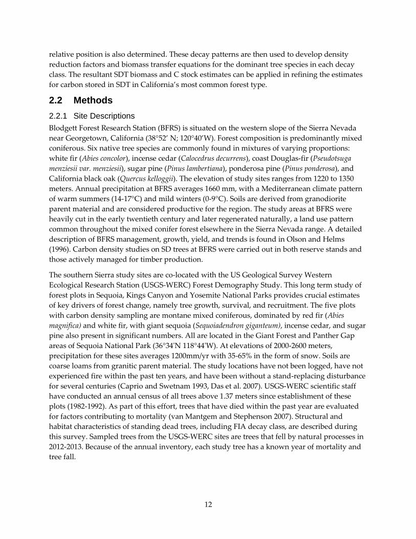
2.2 Methods
2.2.1 Site Descriptions
Blodgett Forest Research Station (BFRS) is situated on the western slope of the Sierra Nevada
near Georgetown, California (38°52’ N; 120°40’W). Forest composition is predominantly mixed
coniferous. Six native tree species are commonly found in mixtures of varying proportions:
white fir (Abies concolor), incense cedar (Calocedrus decurrens), coast Douglas-fir (Pseudotsuga
menziesii var. menziesii), sugar pine (Pinus lambertiana), ponderosa pine (Pinus ponderosa), and
California black oak (Quercus kelloggii). The elevation of study sites ranges from 1220 to 1350
meters. Annual precipitation at BFRS averages 1660 mm, with a Mediterranean climate pattern
of warm summers (14-17°C) and mild winters (0-9°C). Soils are derived from granodiorite
parent material and are considered productive for the region. The study areas at BFRS were
heavily cut in the early twentieth century and later regenerated naturally, a land use pattern
common throughout the mixed conifer forest elsewhere in the Sierra Nevada range. A detailed
description of BFRS management, growth, yield, and trends is found in Olson and Helms
(1996). Carbon density studies on SD trees at BFRS were carried out in both reserve stands and
those actively managed for timber production.
The southern Sierra study sites are co-located with the US Geological Survey Western
Ecological Research Station (USGS-WERC) Forest Demography Study. This long term study of
forest plots in Sequoia, Kings Canyon and Yosemite National Parks provides crucial estimates
of key drivers of forest change, namely tree growth, survival, and recruitment. The five plots
with carbon density sampling are montane mixed coniferous, dominated by red fir (Abies
magnifica) and white fir, with giant sequoia (Sequoiadendron giganteum), incense cedar, and sugar
pine also present in significant numbers. All are located in the Giant Forest and Panther Gap
areas of Sequoia National Park (36°34'N 118°44'W). At elevations of 2000-2600 meters,
precipitation for these sites averages 1200mm/yr with 35-65% in the form of snow. Soils are
coarse loams from granitic parent material. The study locations have not been logged, have not
experienced fire within the past ten years, and have been without a stand-replacing disturbance
for several centuries (Caprio and Swetnam 1993, Das et al. 2007). USGS-WERC scientific staff
have conducted an annual census of all trees above 1.37 meters since establishment of these
plots (1982-1992). As part of this effort, trees that have died within the past year are evaluated
for factors contributing to mortality (van Mantgem and Stephenson 2007). Structural and
habitat characteristics of standing dead trees, including FIA decay class, are described during
this survey. Sampled trees from the USGS-WERC sites are trees that fell by natural processes in
2012-2013. Because of the annual inventory, each study tree has a known year of mortality and
tree fall.

13
2.2.2 Sampling Regime
2.2.2.1 Selection and Standing Dimensions
Standing dead trees were identified at BFRS and in the USGS-WERC study areas through use of
previous inventories and the observations of site managers. From these candidate SD trees,
trees were selected for the study to maximize sampling across FIA decay classes 1-5, to include
individuals across a range of diameters above 20cm at breast height, and to represent all major
species present in the mixed conifer forest. Specifically excluded were trees where fires were a
contributing factor in mortality, and also excluded trees with severe mechanical wounds from
logging operations. Study trees at BFRS were standing during selection and field data
collection, then felled for further measurement and sampling. Study trees in USGS-WERC areas
were the product of natural treefall and were measured while prone.
Each SD tree in the study was classified according to the USFS FIA program’s decay class
system (Figure 2). This classification is based upon the structure and condition of the tree’s top,
branches and twigs, bark, sapwood, and heartwood, and is used for SD trees throughout the
FIA’s nationwide forest inventory plots. (USFS 2010, after Thomas 1979). In addition to decay
classification, upright measurements included diameter at breast height, percent bark present,
height, proximal cause of death, limb and twig condition, wood hardness, use by woodpeckers,
and cavity count. This data was collected according to the Blodgett Forest Inventory Protocol
(Blodgett Forest 2008). Because broken and decaying treetops take on many forms, broken boles
were further classified using four standard shapes: intact, flat (a horizontal break), tapered
(remnant portion of bole tapers to a point), and stairstep (remnant portion of bole tapers
naturally and upper break is flat). This classification permits later estimation of the wood and
bark volume represented in the odd wood volumes resulting from breakage, and the
development of accurate structural loss adjustments for mixed conifer species. The dimensions
of SD treetops were obtained using a sonic Vertex hypsometer (Haglöf Inc., Madison, MS) and a
Criterion 400 Laser (Laser Technology, Inc. Centennial, CO). For trees with broken boles, the
remnant portion was estimated as a percentage (nearest 10%) of original volume; dimensions of
broken portions were measured to the nearest 0.5 meter. Following upright measurements, the
selected SD trees were carefully felled by a professional sawyer. Felling SD trees can be
extremely hazardous, so the sawyer was able to exclude any tree deemed unsafe. After felling,
each tree’s location and felled condition was noted.

14
Figure 2: Forest Inventory and Analysis Decay Class Framework
Decay class
Limbs and branches
Top % Bark
Remaining Sapwood presence
and condition*
Heartwood condition*
1 All present Intact/
pointed 100
Intact; sound, incipient decay,
hard, original color Sound, hard, original color
2 Few limbs,
no fine branches
May be broken
Variable
Sloughing; advanced decay,
fibrous, firm to soft, light brown
Sound at base, incipient decay in outer edge of
upper bole, hard, light to reddish brown
3 Limb stubs
only Broken Variable
Sloughing; fibrous, soft, light to reddish
brown
Incipient decay at base, advanced decay
throughout upper bole, fibrous, hard to firm,
reddish brown
4 Few or no
stubs Broken Variable
Sloughing; cubical, soft, reddish to dark
brown
Advanced decay at base, sloughing from upper bole,
fibrous to cubical, soft, dark reddish brown
5 None Broken Less than 20 Gone
Sloughing, cubical, soft, dark brown, OR fibrous, very soft, dark reddish
brown, encased in hardened shell
*Characteristics are for Douglas-fir. Dead trees of other species may vary somewhat. Use this only as a guide.
Source: USDA Forest Service 2010
2.2.2.2 Dimensional Analysis
Standing dead trees are often host to a wide range of wood conditions, ranging from sound to
extensive decay. The measurements and tissue sampling of felled SD trees were designed to
capture the patterns and variation in this heterogeneity from tree base to top and exterior to
interior. The measurement and sampling protocol builds upon dimensional analysis techniques
and earlier work with both standing dead and down dead wood inventories (Harmon et al.
2011, Whittaker and Woodwell 1968). Felled trees were first marked into 1-3 sections dependent
on size: for logs 0-2m, 1 section; 2-10m, 2 sections; and over 10m, 3 sections. Entire SD volume
was measured by length and the diameters at each section boundary. All diameters were noted
as bark on or bark off. The base section was 2m in length and upper sections divided the

15
remaining length equally; this arrangement was designed to describe wood condition at the
forest floor and as affected by root pathogenic fungi as compared to that at canopy level. Then,
the dimensions and attributes of each section diameter, length, bark thickness, bark presence
(nearest 5%), wood hardness (1-5 scale) were measured. The length to highest intact diameter
and form of the bole above this point was recorded for purposes of describing wood volume.
Following bole volume measures the felled trees were dissected to assess longitudinal and
radial variation in tissues (Figure 3). The same tree sections were used, with wood and bark
samples taken from the midpoint of each section whenever feasible. First, using hand tools or a
chainsaw (Stihl Model MS362), a 5-15 cm cross sectional sample, or “cookie” was cut from the
midpoint of each log section. This cut also provided a clean cross-sectional face to examine
radial decay. The wood condition of the face was described by means of three pith-to-bark
radial transects, the first random and others at 120° and -120° from the first. Each transect was
segmented and measured according to the wood type at the surface. Structurally sound wood
with limited galleries and decay present was classified “hard”. Wood delaminated along one or
more axes, unable to hold its form under pressure, or with many galleries and extensive decay
was classified “soft”. Internal cavities, excavations, or galleries greater than 0.5 cm on the
transect were classified “gone” (density=0). Wood type determinations were made by using a
chaining pin, axe, or small knife to penetrate and dissect adjacent tissue. As a check of the radial
transects, a visually estimate of the total cross sectional area in each wood type (nearest 5%) was
also recorded.
Samples of bark and of each wood type present in each section were obtained in order to
measure SD tree tissue density and carbon content. Hard wood samples were collected as whole
or partial cookies. Bark samples averaged 130 cm3. For soft wood, the green volume was
measured in the field to the nearest millimeter using a ruler or calipers (average sample volume
= 640 cm3). Sample cutting and trimming with a knife or fine saw was conducted on a clean, flat
surface to avoid mixing the soft tissues among trees or sections. For extremely soft wood, a
measured area was marked on an intact surface then excavated into a sample bag (Figure 3).
Finally, all friable samples were transferred to labeled bags for transport to the lab.

16
Figure 3: Technique for Dimensional Analysis; Sampling and Measuring Volume of Decayed Wood
Art credit: S. Cousins
17
2.2.2.3 Wood Volume and Density Determinations
Tissue samples arrived from the field as pre-cut soft wood samples, hard wood cross sections
(full or partial), and bark from each section. Prior to drying, green volume was measured. Hard
wood samples were cut into radial blocks using a 12-inch miter saw (Hitachi C12FDH) and
custom jig, and then measured with a ruler or calipers. Green volume of hard blocks averaged
170 cm3. Due to its irregular shape and absorbent properties, the volume of bark samples was
determined using displacement in water. First, bark samples were fully saturated by repeated
submersion and tracking the volume of water displaced at each iteration. Then, the total volume
of displaced water was determined using a displacement vessel (volumetric edema gauge
(Baseline Evaluation Instruments, White Plains, NY)) or overflow canister (Scientific Equipment
of Houston)). The displaced water was collected and weighed to the nearest 0.1 mL on a balance
(Model P1200-00V1, Sartorius AG, Goettingen, Germany) to determine mass and thus the
volume of the bark sample. All wood and bark samples were then transferred to Kraft paper
bags and placed in a drying oven at 100-105°C; a small number of bark samples were dried at
80°C. After 48 hours, the samples were weighed at intervals of 24-96 hours and removed when
they reached a constant dry weight (Bergman 2010). Wood and bark density was calculated as
the ratio of oven dry mass (g) to green volume (cm3) at room temperature. This value can also
be interpreted as the basic specific gravity (Williamson and Wiemann 2010).
The majority of dried samples, representing trees from all species and decay classes, were then
finely ground for chemical content analysis. Samples were ground using a #4 Wiley mill fitted
with a 0.5 mm screen. If needed, fibrous remains were ground in a small coffee mill. The
resultant powder was thoroughly mixed, and a minimum of 3g retained for analysis. The
University of California Davis Analytical Laboratory (UCDAL) performed analysis of total
carbon and nitrogen presence by weight. The analytical method used was sample combustion in
a muffle furnace, which converts organic and inorganic substances into gases. The gases are
detected and measured by thermal conductivity/IR detection using a TruSpec CN Analyzer
(Leco Corporation, St. Joseph, MI)(Association of Analytical Communities 2006).
2.2.3 Allometric Scaling
Standing dead tree carbon density and density reduction factors are dependent upon both the
quantity (volume) and quality (density and chemical composition) of wood and bark in SD
trees. Both are subject to processes of weathering and decay, which is known to affect a tree’s
many tissues and structural components in different ways. Therefore, density and carbon
content of individual trees were calculated specific to tree section and tissue type. First, total
bark-off tree volume was calculated using measured diameter and height in combination with
taper equations specific to mixed conifer species observed in the Sierra Nevada (Biging 1984).
When total tree height was unavailable (i.e., the bole was broken), SD tree heights were
regressed from diameter using the model ln(Ht) = B0 + B1*ln(DBH) + B2*ln(DBH)*ln(DBH) with
coefficients specific to BFRS (Holmen, unpublished data, 1990). The resulting total SD volume
was allocated to each section and wood type based on the section measurements and radial
transects described above. The surface area per type at the midpoint cross section was
calculated to determine the volume of each wood type specific to section. To do so, distance
along the transect (nearest 0.5cm) was treated as a partial (1/3) annulus, and the proportion of

18
each tissue (wood hard, soft, or gone) was formed by the weight of annulus areas. The mean of
the three sectors on each radial transect formed the section’s surface area. Next, a weight (0.0 –
1.0) was assigned to each wood type within each tree section. Bark volume was later added to
each section in proportion to volume, measured midpoint bark thickness (nearest 0.1mm), and
bark presence while standing (nearest 5%).
2.2.4 Whole Tree Biomass, Density Reduction Factors and Carbon Density
Tissue density and composition were tied directly to measured volumes in individual trees and
their spatially explicit biomass components. In determining whole tree biomass and carbon
content, weights for each wood type (hard, soft, or gone) by section were first used to
reconstruct volume present by type. Biomass per tissue type (kg) is the product of volume and
density, with measurements specific to the samples from that section. Carbon content was then
calculated as the product of tissue type biomass and carbon concentration by weight, which was
also analyzed specific to sample and section. Finally, whole tree biomass and carbon content are
the sum of the component sections. Whole tree density and carbon concentrations are calculated
from the total SD volume and total biomass and carbon content, respectively. A density
reduction factor (DRF) was then computed for each SD tree. DRF is the ratio of dead density to
live density for a tree of equal volume (Harmon et al. 2011). Density reduction factors reported
by tree species and decay class are the mean of individual trees within each group.
2.2.5 Analysis
Because users of density and carbon content measurements may aggregate this data in a
number of ways, the SD tree analysis was compiled using a variety of common aggregation
levels and dependent variables. Response variables include wood and bark density, wood and
bark carbon concentration by weight, total wood biomass, and total wood carbon. These were
examined in groups according to FIA decay class, tissue (wood and bark), position, and taxon.
2.3 Results
2.3.1 Volume and Wood Density Loss
The SDT sampled in the study represent all six major mixed conifer species in each of five FIA
decay classes across broad range of sizes (Table 1). Notably, of 109 total SDT measured and
sampled, 31 are assigned to decay class 4 and 17 to decay class 5. These are the most advanced
decay conditions, and therefore the rarest and least studied SD trees. The sampled standing
dead trees represent the bulk of standing dead biomass in mixed conifer forests: all are over
12.5cm (5 inches) DBH and 95% measure between 20cm and 100cm DBH.
As anticipated, wood density of SDT declined with decay class (Table 2). Live wood density for
the six mixed conifer species ranges from .34 (incense cedar) to .45 (Douglas fir) g/cm3 (Forest
Products Laboratory 2010). From all trees sampled, mean live density was 0.376 g/cm3.

19
Table 1: Standing Dead Tree Characteristics by Species, Decay Class, and Diameter Class
Species Decay class (n) Diameter class (cm DBH) Total
SD Trees 1 2 3 4 5 12.5-30 30-50 >50
White fir 5 6 4 10 4 10 10 9 29
Red fir 6 3 0 1 0 4 3 3 10
Incense cedar 0 4 6 3 3 10 5 1 16
Sugar pine 6 1 4 2 2 3 6 6 15
Ponderosa pine 3 1 6 8 5 5 14 4 23
Douglas-fir 4 0 2 7 3 4 6 6 16
All species 24 15 22 31 17 36 44 29 109
Standing dead trees in decay class 1 were only slightly lower density, averaging 0.36 g/cm3.
Each class progressively decreased, with decay class 5 averaging .21 g/cm3. Across all species,
DRFs followed the same pattern, declining from near-live density (DRF=0.95; class 1) to close to
half of live wood density (DRF=0.55; class 5). Among decay classes, class 3 showed the highest
standard error in both density and resulting DRF (DRF SE=0.06), followed by classes 5 and 4
(DRF SE=0.05 and 0.04).
The pattern of density decrease was most evident in white fir, Douglas fir, ponderosa pine, and
sugar pine (Table 3, Table 4). Each of these species demonstrated a marked decline from decay
classes 1-3 to classes 4-5. White fir and Douglas fir had greater density losses at decay class 5
(DRF= 0.43 ± 0.05 and DRF=0.37± 0.03) than did either of the pines. Incense cedar did not show
declines in density: wood samples from decay classes 4-5 were in fact more dense than live
wood on average. Red fir had too few samples in advanced decay (n=1) to determine a trend.
Table 2: Mean Combined Standing Dead wood and Bark Density and Dead:Live Density Ratio for Each Decay Class
Decay class SD density
(g/cm3)
SE Dead:live*
density ratio SE n
1 0.36 0.01 0.95 0.03 24
2 0.33 0.01 0.88 0.02 15
3 0.29 0.02 0.81 0.06 22
4 0.25 0.02 0.65 0.04 30
5 0.21 0.02 0.55 0.05 16
*Live density, Miles and Smith 2009. All other data this study

20
Figure 4. Density (g cm-3) of Decay Classes 1-5 by Tree Taxonomic Group
2.3.2 Carbon Concentration and Total Carbon Biomass as a Function of Species and Decay Class
Wood and bark from all sections of 76 SDT representing six species and five decay classes were
sampled for carbon and nitrogen concentration of tissues by weight. Across all sampled SDT, C
concentration of combined wood and bark tissues climbed two to three percent by the final
decay class (Table 3). White fir and Douglas fir demonstrated the largest changes. Ponderosa
and sugar pine also showed increased C concentration, with slightly greater variation between
decay classes (Table 6). Standing dead incense cedar maintained a constant carbon
concentration of 0.52 in all decay classes. As with density, the change from live wood conditions
was characterized by calculating the ratio of live C concentration to that of SD, forming a C
concentration adjustment factor. When compared to an assumed live C concentration of 0.50,
early-stage decay SDT (classes 1-3) were uniformly higher in C than live trees (adjustment factor
> 1.00). Standing dead trees in advanced stages of decay (classes 4-5) were higher still, with
adjustment factors ranging from 1.03 to 1.06.
21
Table 3: Mean Combined Standing Dead Wood and Bark Carbon Concentration and Dead:Live Carbon Concentration Ratio for Each Decay Class
Decay class SD Carbon conc. (%)
SE Dead:live* C conc. ratio
SE n
1 51.37 0.24 1.03 0.00 11
2 51.45 0.23 1.03 0.00 10
3 51.51 0.21 1.03 0.00 14
4 52.72 0.28 1.05 0.01 27
5 53.71 0.54 1.07 0.01 14
*Live carbon concentration 50%
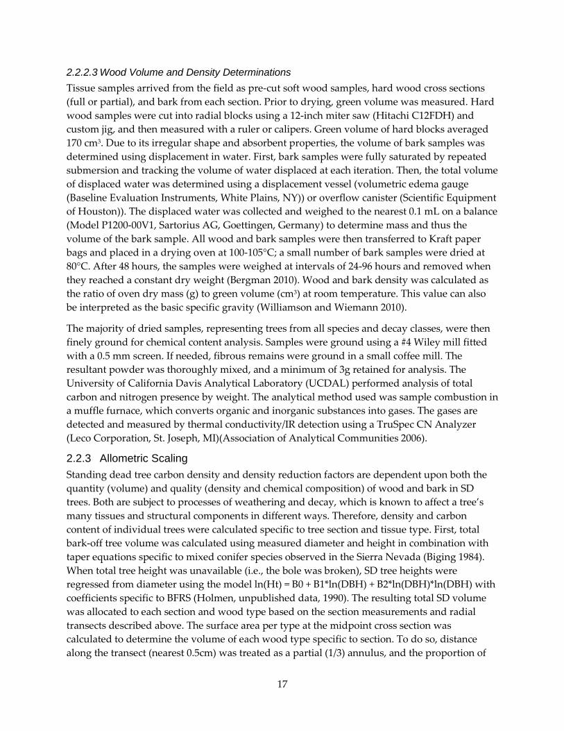
Figure 5: Carbon Concentration of Decay Classes 1-5 by Tree Taxonomic Group
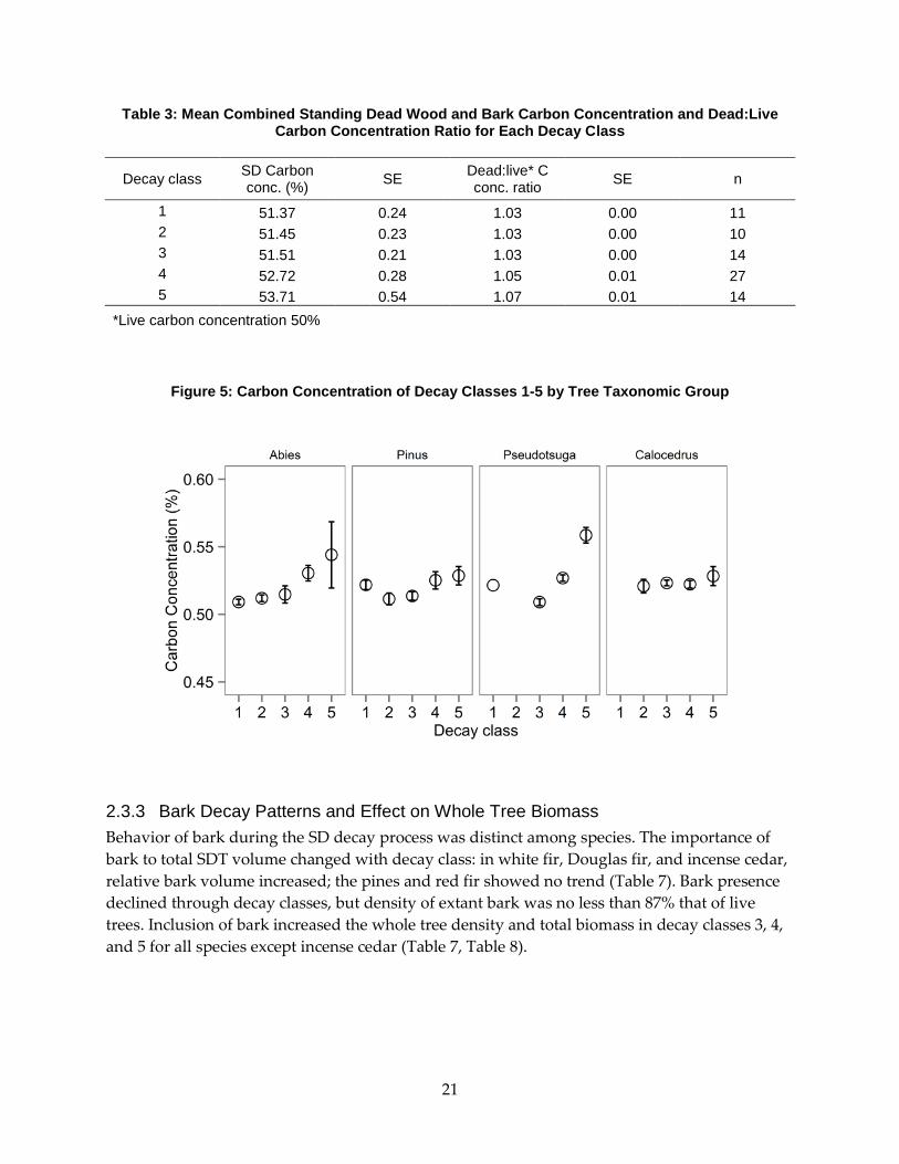
2.3.3 Bark Decay Patterns and Effect on Whole Tree Biomass
Behavior of bark during the SD decay process was distinct among species. The importance of
bark to total SDT volume changed with decay class: in white fir, Douglas fir, and incense cedar,
relative bark volume increased; the pines and red fir showed no trend (Table 7). Bark presence
declined through decay classes, but density of extant bark was no less than 87% that of live
trees. Inclusion of bark increased the whole tree density and total biomass in decay classes 3, 4,
and 5 for all species except incense cedar (Table 7, Table 8).

22
Table 4: Wood Characteristics: Mean Standing Dead: Live Density Ratio and Mean Carbon Concentration for Each Decay Class
Decay class DRF (Dead:live*
density) SE n
Carbon concentration
SE n
1 0.90 0.04 24 0.51 0.00 11
2 0.84 0.03 15 0.51 0.00 10
3 0.81 0.06 22 0.51 0.00 14
4 0.62 0.05 30 0.52 0.00 27
5 0.53 0.05 16 0.53 0.01 14
*Live wood density, Miles and Smith 2009; all other data this study.
Species listed separately in Table 7
Table 5: Bark Characteristics: Mean Standing Dead:Live Density Ratio and Mean Carbon Concentration for Each Decay Class
DRF (Dead:live* density)
SE n Carbon
concentration SE
Number of trees
1.17 0.06 24 0.53 0.00 11
1.01 0.04 15 0.53 0.00 10
0.96 0.06 21 0.53 0.00 13
0.92 0.04 27 0.55 0.00 25
0.87 0.08 10 0.57 0.01 9
* Live bark density, Miles and Smith 2009; all other data this study.
Species listed separately in Table 8
2.3.4 Net Change in Biomass and Carbon Stored
Decay in SDT is a combined pattern of substantial density loss and a subtly increasing C
concentration. The net result is an overall loss of C as decay advances. Relative to live trees, C
content (mean kg/tree) declines even in the first decay class (Table 3). For all species, SDT in
classes 1 and 2 contained 92% of live tree carbon. Through the course of decay this dropped to
64% (class 4) and eventually 51% (class 5) of live tree carbon. Thus, although the chemical
composition of wood and bark is altered by decomposition, the physical pattern of declining
wood density drives loss of nearly 50% of carbon biomass in the most decayed SDT.

23
Table 6: After Density Losses and Carbon Gains, Mean Dead:Live Net Carbon Ratio of Combined Wood and Bark for Each Decay Class
Decay class Dead:live* net C ratio SE Number of trees
1 0.94 0.04 11
2 0.89 0.03 10
3 0.85 0.07 14
4 0.68 0.05 27
5 0.60 0.06 14
*Live carbon concentration 50%
Figure 6: Standing Dead Tree Carbon Concentration, Density (DRF), and Net Carbon Density Relative to Live Trees for Each Decay Class
Ratios are mean standing dead value: mean live value (Miles and Smith 2009). Density values are from measured SDT (n=107); carbon concentration and net carbon density values from SDT (n=76) resampled by Monte Carlo simulation. Error bars are standard error for all measurements.
2.4 Discussion
2.4.1 Patterns in Biomass Loss
The trend of biomass loss measured in SDT from California mixed conifer forests is consistent
with the range of observations for similar species and ecosystems (Harmon et al 2011, Domke et
al 2011). The results confirm that declines in density drive progressive losses of biomass as SDT

24
move through the structure-based decay classes used nationwide by the FIA program. When
these density reduction factors and net biomass changes are coupled with comprehensive live,
SD, and coarse woody debris inventory through time the complete picture of carbon dynamics
in California mixed conifer forests is realized.
White and red fir, Douglas fir, and ponderosa and sugar pine followed similar patterns of
decomposition and density loss, losing nearly half of their live wood density. The true and
Douglas firs advanced in physical decay and weathering more rapidly than pines, but retained
sound bark well into decay classes 4 and 5. Standing dead pines lost bark rapidly; foraging,
especially by woodpeckers and insectivorous mammals, may be a contributing factor in this
trend. Pines maintained harder, more sound wood with occasional fissures and insect galleries,
while firs exhibited delaminated and softening tissues. Standing dead incense cedar was
remarkably resistant to changes in density, consistent with its unique chemical and physical
characteristics (McDonald 1973). Past observations of incense cedar decay in the Sierra Nevada
(Harmon et al. 1987) suggest that this species maintains wood density well into advanced decay
stages, even in pieces of coarse woody debris on the forest floor. Furthermore, the predominant
cause of death for incense cedar at this research site is physical, particularly snow damage
(Schurr 2005). Accordingly, the SDT surveys did not locate a single class 1 incense cedar > 12.5
cm DBH (Table 1). Trees that enter the SD pool by breakage can advance to class 3 or 4 simply
by virtue of their broken boles without any concomitant loss in density, and due to the wood’s
high resistance to decay, can remain intact for many years.
2.4.2 Attribution of Carbon Loss: Volume Loss vs. Decay
Carbon concentration’s gradual increase with decay class is likely caused by the decomposition
activity of brown-rot fungi. Brown rot fungi are among the primary decomposers of wood and
bark in gymnosperms but are unable to digest lignin. As decay progresses, biomass stored as
digestible hemicellulose and cellulose is decomposed preferentially, with lignin-enriched
tissues left behind. Because lignin has a higher C content than the other polymers that make up
wood and bark, the resulting decayed matter also has greater C per unit biomass (Gilbertson
1980, Harmon et al 2013). This explanation is consistent with the pattern observed in incense
cedar, a species resistant to almost all fungal onslaughts (McDonald 1973).
2.4.3 Evaluation of Uncertainty
Uncertainty of DRF and other tissue characteristics was higher in middle decay classes. This
higher uncertainty is likely attributable to greater heterogeneity in the range of conditions of
these SDT. Trees in decay class 1 are essentially intact, while those in class 5 are broken and
often thoroughly decayed. The descriptions of class 3, and to a lesser extent classes 2 and 4,
encompass a wide range of structural and decay conditions. Though the decay class system is
deployed across all species and regions, it was developed on the basis of a single species
(Douglas fir) and is best suited to similar species (USDA Forest Service 2010, Thomas 1979). The
observed uncertainty patterns likely reflect the flexibility of this five-class system and its
suitability to the allometry of mixed conifer species.
The following chapter examines the longevity of SDTs in mixed conifer forests, reporting the
fall rates of SDT on an annual basis. This information complements the pattern of individual

25
tree decay to quantify not only the degree but also the duration of carbon storage and loss by
SDT.
Table 7: Properties of Standing Dead Trees (wood and bark combined) for All Species and Decay Classes Sampled
Species Decay class
SD density (g/cm
3)
Dead:live* density ratio
n (trees)
SD Carbon conc. (%)
Dead:live** net C ratio
n (trees)
white fir 1 0.37 (0.03) 0.92 (0.08) 5 0.51 (0.01) 0.86 (0.10) 3
white fir 2 0.35 (0.02) 0.86 (0.04) 6 0.51 (0.01) 0.84 (0.13) 2
white fir 3 0.29 (0.08) 0.72 (0.19) 4 0.51 (0.01) 0.90 (0.01) 2
white fir 4 0.22 (0.02) 0.56 (0.04) 10 0.53 (0.01) 0.60 (0.04) 9
white fir 5 0.17 (0.01) 0.43 (0.02) 3 0.54 (0.02) 0.46 (0.05) 2
red fir 1 0.38 (0.02) 1.01 (0.04) 6 0.51 (0.00) 0.97 (0.02) 4
red fir 2 0.37 (0.00) 0.98 (0.02) 3 0.51 (0.00) 1.00 (0.01) 3
red fir 4 0.40 (NA) 1.05 (NA) 1 0.52 (NA) 1.10 (NA) 1
incense cedar 2 0.28 (0.02) 0.85 (0.05) 4 0.52 (0.01) 0.84 (0.03) 3
incense cedar 3 0.29 (0.03) 0.91 (0.09) 6 0.52 (0.00) 1.02 (0.13) 3
incense cedar 4 0.30 (0.03) 0.93 (0.10) 3 0.52 (0.00) 0.97 (0.11) 3
incense cedar 5 0.30 (0.03) 0.86 (0.08) 3 0.53 (0.01) 0.91 (0.10) 3
sugar pine 1 0.34 (0.04) 0.99 (0.10) 6 0.52 (0.00) 1.09 (0.07) 2
sugar pine 2 0.26 (NA) 0.76 (NA) 1 0.52 (NA) 0.79 (NA) 1
sugar pine 3 0.26 (0.05) 0.76 (0.16) 4 0.52 (0.00) 0.79 (0.17) 4
sugar pine 4 0.26 (0.03) 0.75 (0.09) 2 0.52 (0.00) 0.78 (0.08) 2
sugar pine 5 0.19 (0.01) 0.55 (0.04) 2 0.52 (0.00) 0.56 (0.04) 2 ponderosa pine 1 0.36 (0.01) 0.96 (0.04) 3 0.53 (NA) 0.98 (NA) 1 ponderosa pine 2 0.34 (NA) 0.91 (NA) 1 0.51 (NA) 0.93 (NA) 1 ponderosa pine 3 0.34 (0.04) 0.89 (0.09) 6 0.51 (0.01) 0.98 (0.03) 3 ponderosa pine 4 0.24 (0.05) 0.63 (0.12) 8 0.53 (0.01) 0.61 (0.18) 6 ponderosa pine 5 0.20 (0.03) 0.52 (0.08) 5 0.53 (0.01) 0.55 (0.12) 4
Douglas-fir 1 0.38 (0.03) 0.85 (0.06) 4 0.52 (NA) 0.74 (NA) 1
Douglas-fir 3 0.21 (0.11) 0.48 (0.25) 2 0.51 (0.00) 0.49 (0.26) 2
Douglas-fir 4 0.26 (0.02) 0.59 (0.05) 6 0.53 (0.00) 0.62 (0.05) 6
Douglas-fir 5 0.19 (0.03) 0.43 (0.07) 3 0.56 (0.01) 0.48 (0.07) 3
*Live density, Miles and Smith 2009. All other data this study
**Live carbon concentration 50% Values in parentheses are standard errors
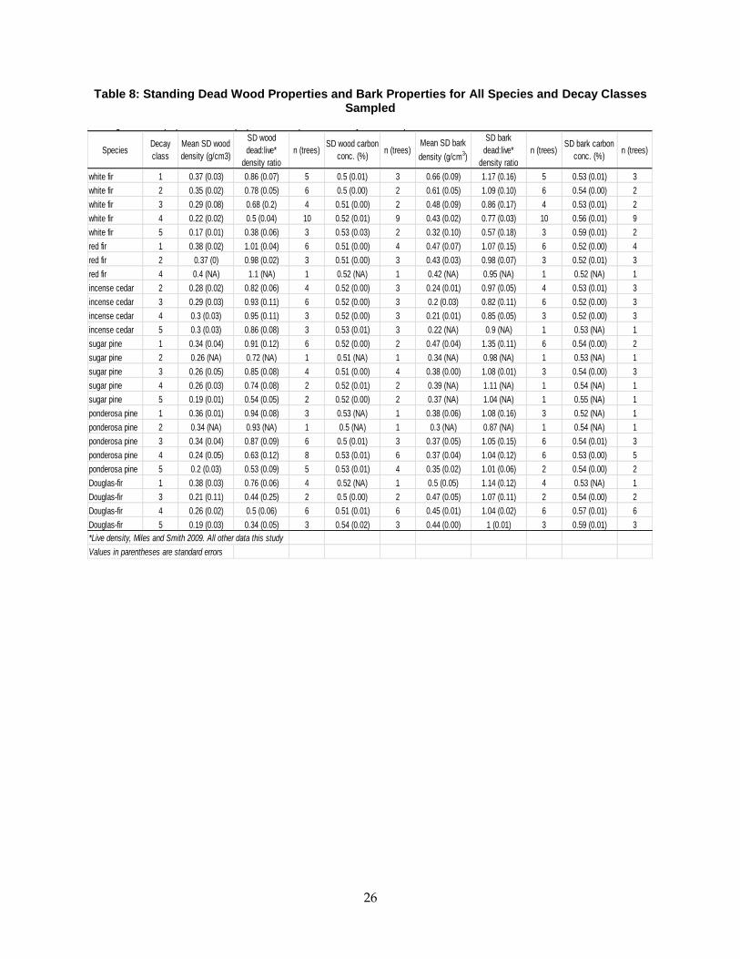
26
Table 8: Standing Dead Wood Properties and Bark Properties for All Species and Decay Classes Sampled
Table NN
SpeciesDecay
class
Mean SD wood
density (g/cm3)
SD wood
dead:live*
density ratio
n (trees)SD wood carbon
conc. (%)n (trees)
Mean SD bark
density (g/cm3)
SD bark
dead:live*
density ratio
n (trees)SD bark carbon
conc. (%)n (trees)
white fir 1 0.37 (0.03) 0.86 (0.07) 5 0.5 (0.01) 3 0.66 (0.09) 1.17 (0.16) 5 0.53 (0.01) 3
white fir 2 0.35 (0.02) 0.78 (0.05) 6 0.5 (0.00) 2 0.61 (0.05) 1.09 (0.10) 6 0.54 (0.00) 2
white fir 3 0.29 (0.08) 0.68 (0.2) 4 0.51 (0.00) 2 0.48 (0.09) 0.86 (0.17) 4 0.53 (0.01) 2
white fir 4 0.22 (0.02) 0.5 (0.04) 10 0.52 (0.01) 9 0.43 (0.02) 0.77 (0.03) 10 0.56 (0.01) 9
white fir 5 0.17 (0.01) 0.38 (0.06) 3 0.53 (0.03) 2 0.32 (0.10) 0.57 (0.18) 3 0.59 (0.01) 2
red fir 1 0.38 (0.02) 1.01 (0.04) 6 0.51 (0.00) 4 0.47 (0.07) 1.07 (0.15) 6 0.52 (0.00) 4
red fir 2 0.37 (0) 0.98 (0.02) 3 0.51 (0.00) 3 0.43 (0.03) 0.98 (0.07) 3 0.52 (0.01) 3
red fir 4 0.4 (NA) 1.1 (NA) 1 0.52 (NA) 1 0.42 (NA) 0.95 (NA) 1 0.52 (NA) 1
incense cedar 2 0.28 (0.02) 0.82 (0.06) 4 0.52 (0.00) 3 0.24 (0.01) 0.97 (0.05) 4 0.53 (0.01) 3
incense cedar 3 0.29 (0.03) 0.93 (0.11) 6 0.52 (0.00) 3 0.2 (0.03) 0.82 (0.11) 6 0.52 (0.00) 3
incense cedar 4 0.3 (0.03) 0.95 (0.11) 3 0.52 (0.00) 3 0.21 (0.01) 0.85 (0.05) 3 0.52 (0.00) 3
incense cedar 5 0.3 (0.03) 0.86 (0.08) 3 0.53 (0.01) 3 0.22 (NA) 0.9 (NA) 1 0.53 (NA) 1
sugar pine 1 0.34 (0.04) 0.91 (0.12) 6 0.52 (0.00) 2 0.47 (0.04) 1.35 (0.11) 6 0.54 (0.00) 2
sugar pine 2 0.26 (NA) 0.72 (NA) 1 0.51 (NA) 1 0.34 (NA) 0.98 (NA) 1 0.53 (NA) 1
sugar pine 3 0.26 (0.05) 0.85 (0.08) 4 0.51 (0.00) 4 0.38 (0.00) 1.08 (0.01) 3 0.54 (0.00) 3
sugar pine 4 0.26 (0.03) 0.74 (0.08) 2 0.52 (0.01) 2 0.39 (NA) 1.11 (NA) 1 0.54 (NA) 1
sugar pine 5 0.19 (0.01) 0.54 (0.05) 2 0.52 (0.00) 2 0.37 (NA) 1.04 (NA) 1 0.55 (NA) 1
ponderosa pine 1 0.36 (0.01) 0.94 (0.08) 3 0.53 (NA) 1 0.38 (0.06) 1.08 (0.16) 3 0.52 (NA) 1
ponderosa pine 2 0.34 (NA) 0.93 (NA) 1 0.5 (NA) 1 0.3 (NA) 0.87 (NA) 1 0.54 (NA) 1
ponderosa pine 3 0.34 (0.04) 0.87 (0.09) 6 0.5 (0.01) 3 0.37 (0.05) 1.05 (0.15) 6 0.54 (0.01) 3
ponderosa pine 4 0.24 (0.05) 0.63 (0.12) 8 0.53 (0.01) 6 0.37 (0.04) 1.04 (0.12) 6 0.53 (0.00) 5
ponderosa pine 5 0.2 (0.03) 0.53 (0.09) 5 0.53 (0.01) 4 0.35 (0.02) 1.01 (0.06) 2 0.54 (0.00) 2
Douglas-fir 1 0.38 (0.03) 0.76 (0.06) 4 0.52 (NA) 1 0.5 (0.05) 1.14 (0.12) 4 0.53 (NA) 1
Douglas-fir 3 0.21 (0.11) 0.44 (0.25) 2 0.5 (0.00) 2 0.47 (0.05) 1.07 (0.11) 2 0.54 (0.00) 2
Douglas-fir 4 0.26 (0.02) 0.5 (0.06) 6 0.51 (0.01) 6 0.45 (0.01) 1.04 (0.02) 6 0.57 (0.01) 6
Douglas-fir 5 0.19 (0.03) 0.34 (0.05) 3 0.54 (0.02) 3 0.44 (0.00) 1 (0.01) 3 0.59 (0.01) 3
*Live density, Miles and Smith 2009. All other data this study
Values in parentheses are standard errors
Standing dead wood properties and bark properties for all species and decay classes sampled

27
CHAPTER 3: Fall Rates of Standing Dead Trees in California Mixed Conifer Forests
3.1 Introduction
…standing dead trees may result from a number of agencies, such as fire, bark
beetles, tree diseases, flooding and drought. Once produced, they become of
concern to foresters…
Keen 1929
Standing dead trees (SDTs) are vital but ephemeral elements of the forest. They represent the
transition from living trees where entropy is actively delayed by the input of energy to coarse
woody debris where the direct contact with soil microbes speeds decay. While they remain
standing, these trees provide essential habitat for wildlife; they store a significant amount of
carbon; and they present potential hazards (Keen 1929, Raphael and White 1984, Hilger et al.
2012).
The rate at which SDTs fall to the ground, referred to as the fall rate, directly influences forest
carbon cycling. Compared to dead and downed trees that interact with the diverse community
of decomposing organisms in the soil, SDTs decay much more slowly (Domke et al. 2011,
Harmon et al. 2011). The carbon loss is attenuated, often for decades, while the trees remain
upright. Since SDTs represent a significant carbon pool in many forests (Hilger et al. 2012),
explicitly accounting for SDT dynamics will improve the estimates of greenhouse gas emissions
as well as the accuracy of forest carbon modeling (Kurz et al. 2009).
Despite their importance, information on SDT fall rates remains relatively sparse (Angers et al.
2010, Parish et al. 2010) with most of the work concentrated in boreal forests. Rates can vary
widely depending on the species, the size, the neighboring forest structure, and the cause of
death (Morrison and Raphael 1993, Garber et al. 2005, Gibbons et al. 2008, Angers et al. 2010,
Parish et al. 2010, Angers et al. 2011). A recent synthesis for North American species reports a
50-fold range in tree fall rates from a minimum of 1.2% yr-1 for spruce trees in Quebec to a
maximum of 54.9% yr-1 for oak trees in South Carolina (Hilger et al. 2012). The dearth of
information is particularly acute for California. There have been only two studies on SDT fall
rates (Table 9): one in the ponderosa pine flats of the Modoc National Forest (Keen 1955) and
the other in the mixed conifer/eastside pine forest of Sagehen Creek Experimental Forest
(Morrison and Raphael 1993). Thus to improve greenhouse gas emission estimates from
California’s forests, a better understanding of the rates and drivers of fall rates for SDTs is
needed.
Toward this end, the investigation capitalized on existing studies at Blodgett Forest Research
Station (BFRS) and Sequoia-Kings Canyon National Parks (SEKI) to examine tree fall rates for
the tree species that comprise the vast mixed conifer forests of California. Specifically, the study

28
developed longitudinal studies where individual trees were tracked over time. Such approaches
provide the best data to quantify patterns and drivers of fall rates (Hilger et al. 2012). The
objectives were to:
1. Determine the overall shape and magnitude of the SDT fall rate curves. Two common
distributions have been noted: a rotated sigmoidal curve (e.g. Angers et al. 2010, Keen
1929) indicating a period of persistence immediately after a tree dies followed by a rapid
increase in fall rate and an exponential curve (e.g., Raphael and Morrison 1987, Hilger et
al. 2012) indicating initial high rates of tree fall followed by a tapering in later years.
2. Quantify species and size differences in SDT fall rate.
3. Compare results for SDT fall rates for California mixed conifer tree species.
3.2 Methods
3.2.1 Site Descriptions
In 1983, Blodgett Forest Research Station established a program to track the fate of standing
dead trees (SDTs). Following the protocols established by Raphael and White (1984), all of the
standing dead trees ≥ 12.7 cm DBH in Compartment 160U were inventoried and tagged.
Compartment 160U (24 ha in size) is typical of the mixed conifer forest in the region. White fir,
ponderosa pine, and incense cedar are the most abundant tree species. Along a low ridge within
the compartment, black oak is locally common. The aspect is predominantly east-facing, with
slopes variable from 5-18% and elevations ranging from to 1220 to 1340 m. Standing dead trees
(SDT) were initially inventoried in 1983. This dead tree inventory was updated in 1989,
1994/1995, and 2005 (Table 9). The site was extensively cut and likely burned in 1913. The forest
was allowed to recover without intervention (except fire suppression) until 1963. Since then, it
has been actively managed using uneven-aged treatment. Major stand entries in Compartment
160U during the inventory period include: sanitation cutting of mistletoe affected trees, 1982;
group selection, 1984; single-tree selection, 1995; and thinning, 2005. Regular clearing for fuel
reduction and safety near roads impacts only a small portion of the compartment.
In 1982 researchers initiated a network of permanent plots in the conifer-dominated forests of
the southern Sierra Nevada to track the fate of individual trees (USGS-WERC Forest
Demography Study). The focus of the demography study is to understand the processes that
influence the recruitment, growth, and mortality of live trees. Toward that end, they maintain
30 large (typically 1 ha), mapped plots selected to be broadly representative of the old-growth
conifer forests found in Sequoia-Kings Canyon and Yosemite National Parks. The work focused
on the 21 plots that included the core species of the mixed conifer forests in the southern Sierra
Nevada, namely white fir, ponderosa pine, sugar pine, incense cedar, Jeffrey pine (Pinus jeffreyi),
red fir, and black oak. These plots spanned an elevational range from 1500 to 2576 m and most
were located in SEKI. The sites were never logged and have not experienced any stand-
replacing disturbances in the last several centuries. Before Euroamerican settlement, low to
moderate intensity surface fires were common. Fire has been excluded since the late 1800’s.
Inventory data indicate that, forest-wide, neither tree density nor basal area have changed

29
substantially during the last two decades (van Mantgem and Stephenson 2007). So for the last
150 years, the dynamics of these forests have largely been governed by local endogenous forces.
3.2.2 Standing Dead Inventories
From 1983 to 2005, BFRS periodically inventoried standing dead trees in Compartment 160U to
complement their overall forest monitoring program (Table 9). This effort was extended in
order to lengthen the record (nearly three decades) and to obtain sufficient data for a
demographic analysis of fall rates. Toward this end, the project completed a thorough census of
the entire 24 ha tract in 2012. In order to efficiently search a large area, the compartment was
divided into three sections. Each section was further broken down into transects 40 meters wide
running East/West across the compartment using flagging to mark the boundaries. A three-
person crew strategically searched the transects for standing dead and fallen trees from
previous inventories as well as trees that had died since the most recent inventory in 2005. The
crew members were spaced 10 meters apart along the southern edge of the East/West transect.
Walking north, each crew member looked for standing and down trees until they reached the
north end of the transect. The crew members then traded places and re-searched this area for
trees that were missed. When the second survey was finished, they moved along the southern
edge of the transect and repeated this search protocol until the section was completed. Such
careful searching is necessary when tracking dead trees. For example, it can be hard to detect a
recently fallen SDT that was severely decayed. Such an individual looks much like coarse
woody debris.
Table 9: Description of Sites/Data from California Conifer Forests Used in This Report
Site Location (county)
Forest type Length of record (years)
Interval Density (SDT ha
-1)
N (trees)
Source
Modoc National Forest
Modoc Mature pine
stands/ beetle kill
30 1919-1949
13.2 (1919)
3,015 Keen 1929; Keen 1955
Sagehen Nevada Mixed conifer/ Eastside pine
10 1978-1998
16.7 (1978)
1,238
Raphael and Morrison
1987; Morrison and Raphael 1993
BFRS El
Dorado
Mixed conifer/ uneven aged management
29 1983-2012
20.0 (1983)
817 This study
SEKI Tulare &
Kern Mixed conifer/
old-growth 31
1982-2013
31.3 (2013)
2,928 This study
Density of standing dead trees (SDTs) is reported with year of the measurement (in parentheses). Modoc NF refers to the Modoc National Forest, Sagehen to Sagehen Creek Experimental Forest, BFRS to Blodgett Forest Research Station, and SEKI to Sequoia-Kings Canyon National Parks.
Another challenge with standing dead tree inventories is that tags secured with nails are more
likely to be lost as the tree decays. Thus care must be taken to distinguish new recruits to the
SDT population (i.e., trees that have died since the last inventory) from trees that lost their tag.
When the crew found a tagless dead tree that included brown needles or fine twigs (evidence of
recent death), the tree was tagged as a new dead tree. When older standing dead trees without
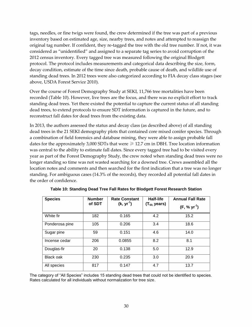
30
tags, needles, or fine twigs were found, the crew determined if the tree was part of a previous
inventory based on estimated age, size, nearby trees, and notes and attempted to reassign the
original tag number. If confident, they re-tagged the tree with the old tree number. If not, it was
considered as “unidentified” and assigned to a separate tag series to avoid corruption of the
2012 census inventory. Every tagged tree was measured following the original Blodgett
protocol. The protocol includes measurements and categorical data describing the size, form,
decay condition, estimate of the time since death, probable cause of death, and wildlife use of
standing dead trees. In 2012 trees were also categorized according to FIA decay class stages (see
above, USDA Forest Service 2010).
Over the course of Forest Demography Study at SEKI, 11,766 tree mortalities have been
recorded (Table 10). However, live trees are the focus, and there was no explicit effort to track
standing dead trees. Yet there existed the potential to capture the current status of all standing
dead trees, to extend protocols to ensure SDT information is captured in the future, and to
reconstruct fall dates for dead trees from the existing data.
In 2013, the authors assessed the status and decay class (as described above) of all standing
dead trees in the 21 SEKI demography plots that contained core mixed conifer species. Through
a combination of field forensics and database mining, they were able to assign probable fall
dates for the approximately 3,000 SDTs that were ≥ 12.7 cm in DBH. Tree location information
was central to the ability to estimate fall dates. Since every tagged tree had to be visited every
year as part of the Forest Demography Study, the crew noted when standing dead trees were no
longer standing so time was not wasted searching for a downed tree. Crews assembled all the
location notes and comments and then searched for the first indication that a tree was no longer
standing. For ambiguous cases (14.3% of the records), they recorded all potential fall dates in
the order of confidence.
Table 10: Standing Dead Tree Fall Rates for Blodgett Forest Research Station
Species Number of SDT
Rate Constant (k, yr
-1)
Half-life (T50, years)
Annual Fall Rate
(F, % yr-1
)
White fir 182 0.165 4.2 15.2
Ponderosa pine 105 0.206 3.4 18.6
Sugar pine 59 0.151 4.6 14.0
Incense cedar 206 0.0855 8.2 8.1
Douglas-fir 20 0.138 5.0 12.9
Black oak 230 0.235 3.0 20.9
All species 817 0.147 4.7 13.7
The category of “All Species” includes 15 standing dead trees that could not be identified to species. Rates calculated for all individuals without normalization for tree size.

31
Table 11: Standing Dead Tree Fall Rates for Sequoia-Kings Canyon National Parks
Species Number of SDT
Rate Constant (k, yr
-1)
Half-life (T50, years)
Annual Fall Rate
(F, % yr-1
)
White fir 1,398 0.0618 11.2 6.0
Ponderosa pine 132 0.0957 7.2 9.1
Sugar pine 540 0.0629 11.0 6.1
Incense cedar 433 0.108 6.4 10.2
Black Oak 128 0.0671 10.3 6.5
Red fir 253 0.0637 10.9 6.2
Jeffrey pine 44 0.0333 20.8 3.3
All species 2,928 0.0708 9.8 6.8
Rates calculated for all individuals without normalization for tree size.
3.2.3 Standing Dead Tree Fall Rate Analysis
For BFRS, the demographic analysis employed non-parametric maximum likelihood estimators
to quantify the fall rate of standing dead trees and then compared rate curves using weighted
log-rank tests. Given the inventory schedule for Compartment 160U, the exact date of fall could
not be determined. Census intervals ranged from 1 year (1994 to 1995) to 10 years (1995 to 2005).
Thus, the data included two kinds of censoring. Some standing dead trees (n = 193) are still
standing (right-censored). For the remainder, only the interval in which trees died (i.e., interval
censoring) was known.
The fall rate functions of standing dead trees for different species were calculated following the
recommendation of two recent reviews of the analysis of interval-censored data (Gomez et al.
2009, Fay and Shaw 2010), using Turnbull’s (1976) generalization of the Kaplan-Meier estimator.
To compare fall curves, the analysis used weighted log-rank tests that employ a permutation
procedure when there are many samples (as in this case). Analyses were implemented in the R
statistical language (R Core Team 2014) using the “interval” library provided by Fay and Shaw
(2010).
For SEKI, given the regular inventory schedule (no interval censoring) and larger dataset,
parametric analysis was used. The approach was to use an accelerated failure time (AFT) model
to quantify fall rates. As described by Parish et al. (2010), AFT considers the distribution for
time to failure (falling in the case of SDTs) conditional on specified covariables (species and size
for SDTs). These covariates act multiplicatively on fall rate time. So conceptually, time to falling
passes quickly or slowly depending on a tree’s covariate values.
Next, the analysis developed competing models that attempt to predict fall rate as a function of
species or size (as measured by DBH) or both species and size. Two function forms were
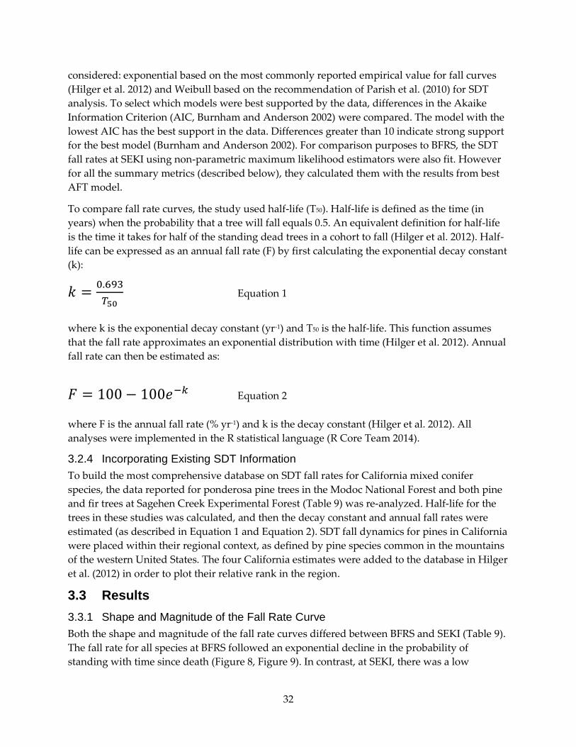
32
considered: exponential based on the most commonly reported empirical value for fall curves
(Hilger et al. 2012) and Weibull based on the recommendation of Parish et al. (2010) for SDT
analysis. To select which models were best supported by the data, differences in the Akaike
Information Criterion (AIC, Burnham and Anderson 2002) were compared. The model with the
lowest AIC has the best support in the data. Differences greater than 10 indicate strong support
for the best model (Burnham and Anderson 2002). For comparison purposes to BFRS, the SDT
fall rates at SEKI using non-parametric maximum likelihood estimators were also fit. However
for all the summary metrics (described below), they calculated them with the results from best
AFT model.
To compare fall rate curves, the study used half-life (T50). Half-life is defined as the time (in
years) when the probability that a tree will fall equals 0.5. An equivalent definition for half-life
is the time it takes for half of the standing dead trees in a cohort to fall (Hilger et al. 2012). Half-
life can be expressed as an annual fall rate (F) by first calculating the exponential decay constant
(k):
Equation 1
where k is the exponential decay constant (yr-1) and T50 is the half-life. This function assumes
that the fall rate approximates an exponential distribution with time (Hilger et al. 2012). Annual
fall rate can then be estimated as:
Equation 2
where F is the annual fall rate (% yr-1) and k is the decay constant (Hilger et al. 2012). All
analyses were implemented in the R statistical language (R Core Team 2014).
3.2.4 Incorporating Existing SDT Information
To build the most comprehensive database on SDT fall rates for California mixed conifer
species, the data reported for ponderosa pine trees in the Modoc National Forest and both pine
and fir trees at Sagehen Creek Experimental Forest (Table 9) was re-analyzed. Half-life for the
trees in these studies was calculated, and then the decay constant and annual fall rates were
estimated (as described in Equation 1 and Equation 2). SDT fall dynamics for pines in California
were placed within their regional context, as defined by pine species common in the mountains
of the western United States. The four California estimates were added to the database in Hilger
et al. (2012) in order to plot their relative rank in the region.
3.3 Results
3.3.1 Shape and Magnitude of the Fall Rate Curve
Both the shape and magnitude of the fall rate curves differed between BFRS and SEKI (Table 9).
The fall rate for all species at BFRS followed an exponential decline in the probability of
standing with time since death (Figure 8, Figure 9). In contrast, at SEKI, there was a low

33
probability of falling for a short time immediately after death (< 5 years) followed by a steeper
rate of fall with time since death (Figure 10, Figure 11, and Figure 12). Thus fall rate curves for
trees at SEKI followed more of a rotated sigmoid distribution. The results from the AFT analysis
confirmed this visual interpretation since the best AFT model used a Weibull distribution as
opposed to an exponential distribution (see below).
Standing dead trees at BFRS fell almost twice as fast as trees at SEKI (Table 10, Table 11). On
average the half-life for SDTs at BFRS was 4.7 years compared to 9.8 years at SEKI. The pattern
held for species-by-species comparison with the exception of incense cedar. At BFRS, the half-
life of incense cedar (8.2 years) was 28% greater than for cedar at SEKI.
3.3.2 Survival Rates of Standing Dead Trees by Species and Size Class
At both BFRS and SEKI, there were significant differences among species. The log-rank test
rejected the null hypothesis of no species differences at BFRS (p < 0.001, Table 10). Incense cedar
had the slowest fall rate at BFRS (8.1 % yr -1); white fir had the fastest (15.2 % yr -1). This
approach could not explicitly test for size effects with a non-parametric approach but the
pattern at BFRS suggested that larger trees stayed standing longer.
For SEKI, there was overwhelming support (the AIC of the best model was 205 points lower
than the next best alternative) for the AFT model that included species, size (as measured by
DBH), and the interaction of species and size. Species identity was the most important covariate
determining fall rate (Table 11). In contrast to BFRS, incense cedar had the fastest fall rate at
SEKI (6.4% yr -1); dead Jeffrey pine trees remained standing for the longest time (F = 20. 8% yr -1).
Fall rates also significantly decreased with increasing DBH for most species (p<0.02). Therefore
to accurately quantify just species differences, predicted fall rates for species holding DBH
constant at 40 cm were calculated (Table 12). However in absolute terms the impact of size was
modest. For example, the predicted half-life for trees with a DBH = 30 cm was 9.9 years and for
a tree twice that size (DBH = 60), it was 10.4 years. Thus a doubling of tree size led to a less than
6% decrease in fall rate. Also in a few species, there was a reversal of the trend – fall rate
increased with increasing DBH. The most pronounced example is ponderosa pine. At a DBH =
40, the half-life for ponderosa pine is 7.7 years (Table 12). At 60 cm (a 50% increase), the half-life
declined by 10% to 6.9 years.

34
Table 12: Standing Dead Tree Fall Rates for Sequoia-Kings Canyon National Parks
Species Number of SDT
Rate Constant (k, yr
-1)
Half-life (T50, years)
Annual Fall Rate
(F40, % yr-1
)
White fir 1,398 0.0624 11.1 6.1
Ponderosa pine 132 0.0904 7.7 8.6
Sugar pine 540 0.0628 11.0 6.1
Incense cedar 433 0.109 6.3 10.4
Black Oak 128 0.0667 10.4 6.5
Red fir 253 0.0621 11.2 6.0
Jeffrey pine 44 0.0336 20.6 3.3
All species 2,928 0.0688 10.1 6.7
Rates have been normalized for trees with diameters at breast height = 40 cm.
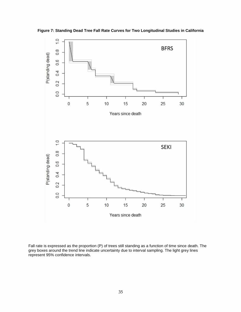
35
Figure 7: Standing Dead Tree Fall Rate Curves for Two Longitudinal Studies in California
Fall rate is expressed as the proportion (P) of trees still standing as a function of time since death. The grey boxes around the trend line indicate uncertainty due to interval sampling. The light grey lines represent 95% confidence intervals.

36
Figure 8: Standing Dead Tree Fall Rate Curves for Three Common Species in Mixed Conifer Forests (white fir, ponderosa pine, sugar pine)
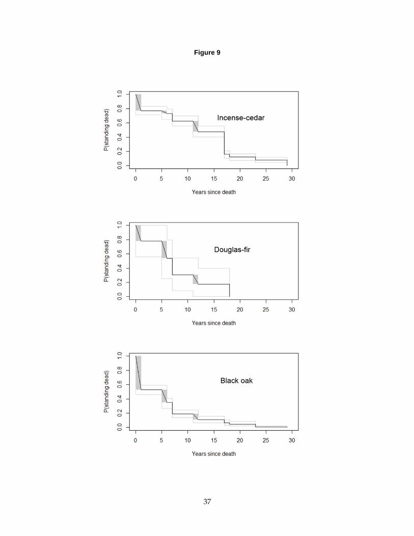
37
Figure 9

38
Figure 9: Standing Dead Tree Fall Rate Curves for White Fir, Ponderosa Pine, and Sugar Pine Trees at SEKI

39
Figure 11
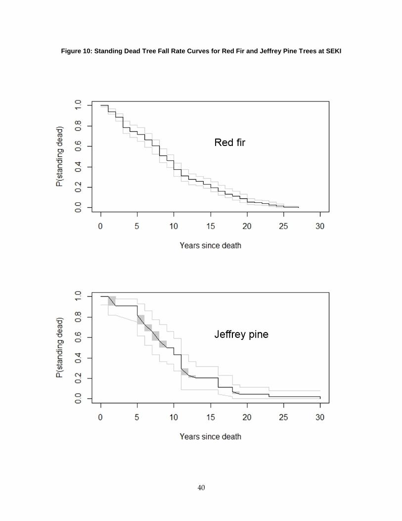
40
Figure 10: Standing Dead Tree Fall Rate Curves for Red Fir and Jeffrey Pine Trees at SEKI
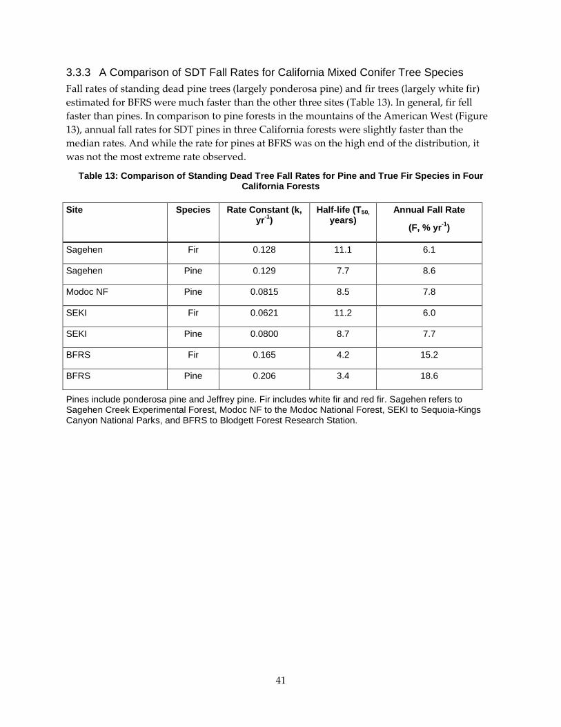
41
3.3.3 A Comparison of SDT Fall Rates for California Mixed Conifer Tree Species
Fall rates of standing dead pine trees (largely ponderosa pine) and fir trees (largely white fir)
estimated for BFRS were much faster than the other three sites (Table 13). In general, fir fell
faster than pines. In comparison to pine forests in the mountains of the American West (Figure
13), annual fall rates for SDT pines in three California forests were slightly faster than the
median rates. And while the rate for pines at BFRS was on the high end of the distribution, it
was not the most extreme rate observed.
Table 13: Comparison of Standing Dead Tree Fall Rates for Pine and True Fir Species in Four California Forests
Site Species Rate Constant (k, yr
-1)
Half-life (T50,
years) Annual Fall Rate
(F, % yr-1
)
Sagehen Fir 0.128 11.1 6.1
Sagehen Pine 0.129 7.7 8.6
Modoc NF Pine 0.0815 8.5 7.8
SEKI Fir 0.0621 11.2 6.0
SEKI Pine 0.0800 8.7 7.7
BFRS Fir 0.165 4.2 15.2
BFRS Pine 0.206 3.4 18.6
Pines include ponderosa pine and Jeffrey pine. Fir includes white fir and red fir. Sagehen refers to Sagehen Creek Experimental Forest, Modoc NF to the Modoc National Forest, SEKI to Sequoia-Kings Canyon National Parks, and BFRS to Blodgett Forest Research Station.
Figure 11. Standing dead tree fall rate curves for incense cedar,
Douglas-fir, and black oak trees at BFRS

42
Figure 12: Distribution of Standing Dead Tree Annual Fall Rates for Pine Species in the Montane Forests of the Western United States (n = 31)
The four sites from California (Table 13) were added to the database compiled in Hilger et al. 2012. The arrows with labels identify the California sites. Calculation methods follow Hilger et al. (2012).
3.4 Discussion
The SDT fall rates measured at BFRS and SEKI fall within the expected range of observations for
similar species in similar forests. Added to the existing data from California and placed within
the context of western mountain forests, these results provide the basis for major improvements
BFRS
Sagehen
BhendFSEKI
Modoc
KI
43
in estimating carbon transfers from SDTs. The results confirmed the expectation that fall rates
would vary by species and size.
However BFRS and SEKI do represent opposite ends of the spectrum of forest structure and
management regime for mixed conifer forests in California. The study site at BFRS is an actively
managed uneven-aged stand while the SEKI plots are in a contiguous old-growth forest. Not
only are individual trees at BFRS on average smaller, a factor contributing to faster fall rates, but
SDTs do tend to fall faster in managed stands even when other factors are held constant (Garber
et al. 2005, Gibbons et al. 2008). It is unclear exactly why this is the case – there are relatively few
studies – but Garber et al. (2005) suggested it might be related to the disturbance associated
with the treatments. BFRS is also a productive site that receives considerably more precipitation
than SEKI (see above) and experiences less water stress (van Mantgem et al. 2007, Eitzel et al.
2013). As Keen (1955) noted, wetter sites in the pine flats had considerably faster fall rates (6.4 %
yr-1) than comparable stands on drier sites (9.8 % yr-1).
Findings from both sites must be interpreted with an appropriate assessment of their
robustness. In the case of BFRS, the results (e.g. Figure 8) reflect the uncertainty introduced by
the varied census schedule. The interval-censoring leads to large errors in the estimates of rate
of fall. In contrast, SEKI conducts annual censuses thereby avoiding issues associated with
interval sampling. However until 2013, SDTs were not explicitly monitored and thus had to be
reconstructed from the location notes the time of fall. There is no means to quantitatively
evaluate errors in this process. However they did record ambiguities in the assignments and
repeated the analysis using the alternative designations. This comparison found no tangible
differences in the fall rate results with the alternative dataset. Given the nature of the
reconstruction, this approach was most likely to underestimate the fall rates. Some downed
trees that were obvious to researchers may not have warranted a location note to inform the
crew of its status. Crews would code such a tree without an explicit note regarding its status as
still being standing. However, the match between the results from SEKI and the other sites in
California (Table 13) does allay potential concern about underestimates.
In the next section, this information on fall rates for SDTs will be combined with the decay
reduction factors and carbon density assessment reported in Chapter 2 to quantify the potential
impact on carbon storage and accounting in mixed conifer forest.

44
CHAPTER 4: Improving California’s Greenhouse Gas Accounting for Forest and Rangelands: Tracking Gains and Losses in the Standing Tree Carbon Pool
4.1 Introduction
4.1.1 Background
The California greenhouse gas inventory consists of annual estimates of emissions to and
removals from the atmosphere for the entire state, produced by the staff of California ARB.
These needs established the operational requirements for the data sources and methods used in
developing the accounting approach for the forests and rangelands of California (Battles et al.
2014). The requirements included:
Complete state coverage
Repeat measurements over time
Continuous data gathering in the future
Conformity to IPCC (2006, 2013b) guidelines
Public availability
Moderate to fine spatial resolution for remote sensing data
Low data processing before analysis
Given IPCC guidelines, the study partitions estimates of forest carbon into the following stocks:
live tree (aboveground and total), standing dead tree, live understory vegetation, coarse woody
debris, and litter. This chapter focuses on the assessment of the standing dead tree pool.
Published vegetation carbon research commonly calculates carbon stocks as the product of
surface areas of land cover types, classified by satellite remote sensing (Table 14), and the
carbon densities, derived from field measurements of trees and allometric equations, summed
over all land cover types (e.g. Achard et al. 2004, DeFries et al. 2007, Harris et al. 2012). The
number of land cover types that satellites with moderate spectral or spatial resolutions can
accurately discriminate, generally five to twenty classes (e.g. Bartholomé and Belward 2005,
Loveland et al. 2000), can limit the possible carbon density assignments to a few discrete values.
In contrast, other methods use Light Detection and Ranging (Lidar) or high-resolution satellites
such as QuickBird, Ikonos, or WorldView (Table 14) to sense the physical dimensions of trees to
which aboveground biomass directly correlates (e.g., Gonzalez et al. 2010, Saatchi et al. 2011).
With these systems, forest carbon content equals the product of the area and the carbon density
of each pixel, where carbon density is calculated by applying allometric equations to field
measurements of individual trees and correlated to canopy height metrics estimated by Lidar or

45
tree crown diameter estimated by high-resolution satellite data. This method generates raster
coverage of the spatial distribution of forest carbon density with continuous values.
Table 14: Summary of Major Remote Sensing Technologies Used for Assessing Carbon Stocks
Sensor Scale Platform Mode Detection Access
MODIS 250 m Satellite Passive 36 spectral bands Public
Landsat 30 m Satellite Passive 9 spectral bands Public
QuickBird 1m Satellite Passive 5 spectral band Commercial
GLAS 1 km Satellite Active Light returns Public
PALSAR 10 m Satellite Active Microwave returns Public
Lidar <1 m Aircraft Active Light returns Commercial
Aerial photos
50 m Aircraft Passive Visible spectrum Public (NAIP)
MODIS = Moderate Resolution Imaging Spectroradiometer; GLAS = Geoscience Laser Altimeter System; PALSAR = Phased Array type L-band Synthetic Aperture Radar; Lidar = Light Detection and Ranging; NAIP = National Agriculture Imagery Program.
A recent meta-analysis of the performance of remote sensors in estimating aboveground forest
biomass/carbon density (Zolkos et al. 2013) concluded that the active sensors were more
accurate than the passive sensors (Table 14). In addition, various implementations of Lidar were
better than any satellite-based active sensing platform. In general, the greater detail with which
the tree form was resolved (e.g., height. crown width), the better the performance. However as
Zolkos et al. (2013) note, the accuracy of the estimate also depended on the field measurements
of tree biomass/carbon.
Estimating the carbon density of standing dead trees (SDTs) poses challenges on both fronts.
They are hard to detect from above and hard to measure in the field. Landsat-based models to
estimate SDT density in Washington and Oregon had poor predictive ability with performance
confounded by the heterogeneity of the SDT population and the difficulty in detecting SDTs
(Eskelson et al. 2012). Even with the most precise sensor (i.e., Lidar), it is difficult to distinguish
live from dead trees (Pesonen et al. 2008), but recent work suggests it is possible to use synoptic
measures of forest structure to predict SDT density. For example, Bater et al. (2009) were able to
achieve reasonable accuracy predicting the proportional density of SDTs in an evergreen conifer
forest in British Columbia using a Lidar-derived measure of the variation in vegetation height.
This result adds further evidence to the potential of laser scanning technology in natural
resource applications. However Lidar is currently too expensive to acquire and process to make
it a viable tool in GHG accounting at regional or national scales (Zolkos et al. 2013, Battles et al.
2014). For example, extrapolating from a recent UC Berkeley/US Forest Service campaign to
acquire Lidar for most of the Tahoe National Forest (3,557 km2 @ $210/km2) puts the cost of
acquiring small-footprint Lidar for the forests and rangelands of California at approximately
$70M. Moreover as was noted in Chapter 2, there is limited information on the carbon density

46
of SDTs. Thus a comprehensive remote sensing effort would need to be matched with a similar
effort on the ground.
4.1.2 Problem Statement
This chapter summarizes efforts to improve the estimation of SDT carbon within the framework
of the GHG inventory development funded by ARB. The inventory development called for an
evaluation of geospatially explicit land use/land cover products and vegetation inventories to
track biomass changes in live vegetation and then an implementation of the best available
approach. As part of the Energy Commission-funded effort, this evaluation and implementation
was extended to include SDTs.
4.2 Methods
(Note that for completeness, some methods first described in Battles et al. 2014 are included
here.)
4.2.1 Developing GHG Accounting Approach
Despite the promise of airborne Lidar to detect both live and dead tree characteristics, the cost
of its acquisition made it impractical for the ARB accounting efforts. As an alternative, other
research (Baccini et al. 2008, Lefsky 2010) has demonstrated the use of laser scanning data from
the ICESat satellite. ICESat Geoscience Laser Altimeter System (GLAS) global altimetry data
(Abshire et al. 2005) is available for selected periods from 2003 to 2009 at 170 m spatial
resolution. It is theoretically possible to take the difference between canopy elevation from
GLAS and ground elevation from the United States Geological Survey (USGS) National
Elevation Dataset (Gesch et al. 2002) at 30 m spatial resolution to calculate canopy height (the
best predictor of live tree biomass, Gonzalez et al. 2010) and variation in forest height (the best
predictor of SDT density, Bater et al.2009). However the ICESat only made 16 passes over
California, covering only a fraction of the area of the state. A complete coverage would have
needed more passes and passes for multiple years. So, GLAS provided insufficient data for this
work. Furthermore, GLAS would have required processing and calibration to field-measured
canopy heights.
High-resolution satellite data from QuickBird, Ikonos, or WorldView is not in the public
domain. This high-resolution data would also have required processing and calibration to field-
measured tree crown diameters and dead tree densities. Given the expense and effort, this
option was also eliminated.
The study assessed different data sources for a land cover approach. Land cover classification
must use identical methods over time and data from different years must be co-registered
geographically (each pixel lines up over time) to permit determination of land cover change
over time. Possible land cover remote sensing options include:
National Aeronautics and Space Administration (NASA) MODIS Land Cover Type
(MCD12Q1, Friedl et al. 2010): annual 2001-2007 (available) and 2008-2010 (planned), 250
m spatial resolution, 17 land cover classes
USGS National Land Cover Database (NLCD, Homer et al. 2007): 2001 and 2006

47
(available) and 2011 (in progress, but not yet available), 30 m spatial resolution, 29 land
cover classes
USGS LANDFIRE vegetation types (Ryan and Opperman 2013): 2001, 2008, 2010
(available), 2012 (planned), 30 m spatial resolution, derived from Landsat satellite data,
163 vegetation type classes in California.
Within a land cover class, it is necessary to use another variable to discriminate different levels
of carbon density within a single year and growth or mortality over different years. Normalized
Difference Vegetation Index (NDVI), an index related to green foliar area (Tucker 1979) and
biomass (Tucker et al. 1985), and net primary productivity (NPP), a measure of annual
vegetation production, are possible variables. Since none of these "green indices" directly sense
the dead trees (no foliage), estimates of SDT biomass would need to rely on establishing
relationships between live tree productivity or biomass and dead tree biomass. Possible
vegetation level remote sensing options include:
NASA MODIS NDVI (MOD13Q1): every 16 days from 2001 to present, 250 m spatial
resolution
USGS WELD NDVI (Roy et al. 2010): annual 2006-2010 (available) and 2011-2012
(planned), 30 m spatial resolution
NASA MODIS NPP (MOD17A2, Running et al. 2004), every 8 days from 2000 to present,
1 km spatial resolution, vegetation production rate (kg m-2 y-1) calibrated to field
measured biomass (Turner et al. 2006)
USGS LANDFIRE vegetation height and cover (Ryan and Opperman 2013): 2001, 2008,
2010 (available), 2012 (planned), 30 m spatial resolution, derived from Landsat satellite
data, 39 height classes and 54 vegetation cover classes in California.
After acquiring and testing different sets of land cover and vegetation level remote sensing, the
advantages of LANDFIRE data became clear. LANDFIRE combines data from several sources to
produce fine-grained spatial units (Rollins 2009) over which field data can be applied. In
addition, the different spatial data layers can be adjusted based on what is known from the field
data. If there is detailed field data (e.g., forests), carbon density assignments can be precisely
resolved. If data is sparse (e.g., shrublands), generic assignments are more appropriate. When
new results become available, the assignments can be improved (e.g., SDT). This matching
allows a core objective to be met, namely to build a data-driven method. LANDFIRE also meets
other project criteria. The USGS has completely processed and calibrated the data against field
measurements, posted the data publicly, and provided three different years with plans for
future releases. Moreover, the LANDFIRE variables are developed together, providing an
internally consistent treatment of land cover and vegetation characteristics.
4.2.2 Estimating Standing Dead Tree Carbon
LANDFIRE assigns an existing vegetation type (EVT) to each pixel that represents the species
composition currently at the site. In natural ecosystems, EVT represents plant community types
that tend to co-occur in environments with similar biophysical characteristics. EVT’s are

48
hierarchical grouped into increasingly coarse units – subclass, class, order – that are consistent
with the National Vegetation Classification System (NVCS, Jennings et al. 2009). The five orders
used by LANDFIRE are defined by the lifeform of the dominant vegetation, namely tree (38% of
the analysis area based in 2008), shrub (35%), herb (15%), no dominant vegetation (5%), and
non-vegetated (6%). In addition to type, LANDFIRE assigns each pixel an existing vegetation
cover (EVC) and existing vegetation height (EVH). EVC is the vertically projected percent cover
of the live canopy layer for a pixel; EVH is the average height of the dominant vegetation. Both
EVC and EVH are expressed as ordinal values. Together these three LANDFIRE products
provide sufficient information to define relatively fine-scale biomass classes.
Given the capacity of LANDFIRE, the authors developed a carbon stock mapping method that
uses a finely resolved stratify and multiply approach. By combining vegetation type, cover, and
height classes, there are 100’s of potential strata. The nature and number of these strata can
greatly reduce within-class variation in carbon density. However these well-defined strata
require sufficient data to “fill” them with estimates of carbon density.
For tree-dominated landscapes in the regional GHG accounting effort, this study relied
exclusively on data from the US Forest Service (USFS) Forest Inventory and Analysis (FIA)
program to calculate carbon density for biomass classes defined by LANDFIRE as tree-
dominated. The FIA program is a statistically sound, national inventory of forest resources that
includes a network of field plots distributed at a density of approximately one plot per 2,492 ha.
Measurements in these plots (Phase 2) include nested sampling of trees (e.g., species
identification, DBH, status, height, and canopy position). In the western United States, FIA plots
are measured on a ten-year cycle. The fraction measured in any individual year is designed to
be a representative sample of all plots in the region (Bechtold and Patterson 2005). Details of the
inventory and access to the data are available online (http://fia.fs.fed.us/, FIADB 2011).
The FIA 2011 database for California (FIADB 2011) served as the forest inventory. This database
included results from plots measured between 2001 and 2009. Exact coordinates of the location
of FIA plots are not publically available. To ensure the accuracy of the biomass densities, the
remote sensing lab of the USFS Region 5 provided 2001 and 2008 LANDFIRE vegetation
classifications (type, subclass, class, and order), cover class and canopy height of each FIA plot
in California using the exact geographic coordinates. They did not release coordinates, only the
LANDFIRE values for the exact plot locations were released.
The FIA program provides plot-level estimates of key forest attributes, including those required
to meet national requirements for GHG reporting (EPA 2013). Forest carbon is divided into the
following pools: live tree (aboveground and total), standing dead tree, live understory
vegetation, coarse woody debris, litter, and soil. Below, the logic and approach to the
measurement of the SDT pool, using strata defined by LANDFIRE and informed by FIA
measurements, are further explained.
This approach to estimating SDT carbon relies on the assumption that the live tree pool is the
primary driver as well as the best indicator of carbon storage in forests (Fahey et al. 2010). At
the most basic level, this assumption is fundamentally true for SDTs since they are created from

49
live trees. However it does not necessarily follow that the features of the live trees sensed by
LANDFIRE (i.e., canopy cover and height) translates directly to the SDT pool. The authors
tested the efficacy of predicting SDT carbon from LANDFIRE attributes by quantifying the skill
with which equations estimate SDT biomass as functions of LANDFIRE canopy cover and
canopy height assignments. The authors focused their efforts on the most abundant forest type
in California -- the vast Sierran mixed conifer forest (21,500 km2). Specifically they compared the
performance of linear, saturating, and power functions. Overall, linear combinations of height
and cover proved to be the best approach. They significantly outperformed power functions
based on model fits. Saturating functions were difficult to estimate given ordinal cover and
height information.
Linear regressions of the general form were fit:
√ Equation 3
where AGSDT is plot-level SDT aboveground biomass (“oven-dry”) density in Mg ha-1, a is the
intercept term; EVC is the upper limit of the LANDFIRE tree cover class (e.g., cover class ≥10%
and < 20% was assigned a value of 20); EVH is the upper limit of the LANDFIRE tree height
class; b and c are coefficients of EVC and EVH; and E is the standard deviation of the regression.
AGSDT was square-root transformed to correct for positive skew in biomass distribution. Positive
skew is a common feature of biological data that is routinely corrected using a square-root
transformation (Sokal and Rohlf 1995).
The authors compared reduced versions of the full linear model using the Akaike’s Information
Criteria (AIC). In total six models were evaluated: EVC only with an intercept term; EVC only
without an intercept term; EVH only with an intercept term; EVH only without an intercept
term; EVC and EVH with an intercept term (the full model, Equation. 3); and EVC and EVH
without an intercept term. AIC difference values (∆AIC), the difference between the AIC value
of a given model (AICi) and the AIC value of the best approximating model (AICmin), were used
to measure the strength of evidence for each model (Burnham and Anderson 2002). Although
the interpretation of ∆AIC’s is subjective, they provide an intuitive assessment of the strength of
support for one model relative to another (Burnham and Anderson 2002). Statistical analyses
were conducted in R (3.1.2).
4.2.3 Incorporation of Revised Estimate (Chapter 2) of Standing Dead Tree Carbon Pools
Another objective was to incorporate improvements in the field assessment of SDT carbon into
the overall GHG budget. As described in Section 2.2.1, the current FIA measurement only
accounts for the volume lost as an SDT weathers. It assumes that the wood density and carbon
content of an SDT remains the same as a live tree, an assumption that can lead to overestimates
by as much as 40% for SDTs in the mixed conifer forest (Table 6). Using the results from
Chapter 2, SDT stocks were calculated for FIA plots in the mixed conifer forest using two
methods: with species-specific reduced density and carbon content according to decay class
(Table 7 and without decay adjustments (FIA reported results). Then the differences across
LANDFIRE cover and height classes were evaluated.

50
4.2.4 Analytical Framework for Projecting Carbon Dynamics of Dead Trees
The death of a tree initiates the inevitable loss of stored carbon but tracking the timing of the
loss is complicated. SDTs emit carbon as they decay while standing. Alternatively, when a SDT
falls, its carbon is re-assigned to the coarse woody debris pool. Thus any projections of SDT
carbon must account for both the weathering and decay rates (Chapter 2) as well as the fall rate
(Chapter 3). As noted above, stresses related to global change have increased forest mortality
rates and consequently increased the amount of carbon stored in SDTs. For example a recent
analysis for the American West concludes that over the last two decades bark beetles haved
killed as many trees as wildfire (Hicke et al. 2013). To gain some perspective on the magnitude
and timing of carbon loss to be expected from a major mortality event, the authors simulated
the carbon dynamics of SDTs following an outbreak that killed 35% of the pine trees, – a
realistic scenario considering that Keen (1929) reported a similar death rate for a pine stand in
California. They generated a representative distribution of pine species and size classes by
starting with the live tree data for all the mixed conifer plots in the FIA database. They then
randomly "killed" 35% of the trees ≥ 12.7 cm in DBH (2,294 dead trees in 766 plots). The authors
used the decay transition probabilites for pine trees 5 years and 10 years after death reported by
Morrison and Raphael (1993). They then applied the correction factors that were developed
(Chapter 2) to assign carbon densities by species and decay class in order to track the loss of
carbon in the SDT pool over a decade.
4.3 Results
4.3.1 Performance of LANDFIRE to Detect Changes in Standing Dead Tree Biomass
Existing vegetation height (EVH) was the best LANDFIRE metric for predicting SDT biomass.
For tree-dominated landscapes (i.e., forests) in general, SDT biomass significantly increased
with increasing EVH. Specifically for the existing vegetation type (EVT) that was classified as
Mediterranean Mesic Mixed Conifer Forest , the best model was dominated by EVH (p<0.001)
but the existing vegetation cover (EVC) was also included in the model with the lowest AIC
(Figure 14). Interestingly SDT biomass declined slightly with increasing EVC (Figure 14B).
While the model captured the general trend as indicated by a significant regression model
(p<0.001), there was a great deal of variation over individual estimates (Figure 14A) which
resulted in a low goodness-of-fit (R2 = 0.03).
As expected, SDT biomass was significantly and postively related to live tree biomass (Figure
15, p < 0.001). However the relationship was relatively weak (R2 = 0.28) particulary when live
tree biomass was low. For example, plots with live tree biomass < 5 Mg ha-1 had SDT biomass
values that ranged from 0 to 105 Mg ha-1.

51
Figure 13: Standing Dead Tree Aboveground Biomass in the Mixed Conifer Forests as a Function of Canopy Cover Class and Height Class for the California Mixed Conifer Forest
A. Estimates from 766 FIA plots. B. Statistical interpolation of results from 766 FIA plots.
4.3.2 Performance of FIA in Estimating Standing Dead Tree Carbon
As documented in Chapter 2, the current FIA method systematically overestimates the carbon
stored in SDTs. For the mixed conifer forest, the magnitude of the overestimate varies with the
EVH and EVC (Figure 16). At the plot level, the overestimate ranged from 6% to 33% with a

52
median of 21%. In absolute terms, the overstimate varied from 0.3 to 4.8 Mg ha-1 (median = 1.2
Mg ha-1).
Figure 14: Relationship Between Aboveground Standing Dead Tree Carbon Density and Aboveground Live Tree Carbon Density for the 766 FIA Plots
Figure 15: Magnitude of the Overestimate in Aboveground Standing Dead Tree Carbon Density as a Function of Canopy Cover and Height Class for the California Mixed Conifer Forest
Results are the statistical interpolation of the differences between FIA carbon density estimates and the results from Chapter 2.

53
4.3.3 Impact of Improvements on Carbon Stocks and GHG Estimates
The regional implications of SDT decay for estimates of aboveground carbon stocks were
examined by comparing the status quo estimate with an alternative, decay-adjusted estimate.
SDT inventory information (volume, species, and decay class) came from 766 FIA plots in
California mesic mixed conifer forests (FIADB, 2011; USGS-LANDFIRE, 2008). In these forests,
SDT volume was dominated by white fir, which totaled 2801 m3 and 38.5% of overall volume.
Following in importance were Douglas-fir and sugar pine, which formed 17.3% and 16.7% of
total SDT volume respectively. The six species included in this study (Chapter 2) accounted for
90.8% of total SDT volume (6778 of 7465 m3). In 2008, mesic mixed conifer forests had a mean
live aboveground carbon density of 117 Mg ha-1, and occupied a land area of 21,500 km2 in
California (FIADB, 2011; USGS-LANDFIRE, 2008). This is California’s single most extensive
forest type and represents 5.3% of the state’s total land area. The decay-adjusted carbon stock of
SDTs in mesic mixed conifer forests was 9.40 Mg C ha-1, for a statewide total of 20.20 Tg. Thus,
the decay-reduced SDT stock amounts to 8% of aboveground live carbon. Using the status quo
approach (i.e., unadjusted) yielded a higher stock estimate: SDTs accounted for 11.16 Mg C ha-1,
and a statewide total of 23.98 Tg. The difference in total carbon stock between the two
estimation methods is 3.79 Tg. In summary, an estimation approach that does not account for
changing net carbon density yields an 18.8% overestimate of extant SDT carbon stock.
4.3.4 Five and Ten-Year Projections of SDT Carbon Storage
In a mortality scenario where 35% of the pine trees were randomly killed, the percentage of
SDTs in the mixed conifer increased from 13.6% of stems to 19.5% and nearly doubled the
fraction of carbon stored in SDTs from 8.7% to 16.1%. In other words it was a major but not
catastrophic shift in forest carbon allocation. The transition probabilities for SDT pine from
Morrison and Raphael (1993) and this study’s decay-adjusted estimates of SDT carbon (Chapter
2) resulted in the rapid loss/transfer of SDT carbon (Figure 17). The initial 17.3 TgC in SDT
created by the simulated beetle-kill declined steeply in the 5-years following death. Most of the
loss was due to treefall – nearly 60% of the SDTs fell within the first five years. During the next
five years the rate of decrease declined but the loss still represented more than a 2x decline in
SDT carbon (Figure 17). In summary, ten years after the end of the outbreak only 8% (1.4 TgC)
of the initial SDT carbon remained in the pool.

54
Figure 16: Decline in the Standing Dead Tree Carbon Pool Following a Simulated Beetle-Attack on Pine Trees in the California Mixed Conifer Forest
4.4 Discussion
4.4.1 Implications of Dead Tree Assessment Strategies to GHG Accounting
The most recent national report of greenhouse gas emissions and sinks (US EPA 2014) relies on
results from the FIA inventory to assess carbon stock changes on forest lands. Given the reliance
on FIA information where the carbon density of standing dead trees is assumed to be the same
as live trees, the carbon stored by decaying SDTs is overestimated. As quantified here for the
mixed conifer forest in California, the extent of the overestimate can be considerable (18.8% for
the SDT carbon pool). Admittedly, SDTs currently account for a relatively small fraction of
forest carbon. So the overestimate is only 1% of the live+dead tree pool. However, the concern is
that SDT fraction has been increasing in Calfornian forests and is likely to continue to increase
(Section 2.1.1). Thus the magnitude of the error in GHG accounting will rise if there is a
continued assumption that SDTs do not begin to decay until they fall to the ground.
This work on the decay patterns for mixed conifer trees represents a major contribution to the
national effort to improve estimates of carbon stored in SDTs (Domke et al. 2011, Harmon et al.
2011). Not only did they increase the number of species with empirical estimates of SDT carbon
by 40%, but they also are the first to sample across the entire decay class gradient. Harmon et
al. (2011) sampled sparingly in the more severe decay classes with no measurements from the
most severely decayed trees. As a first approximation, they suggest using the reduction factor
for decay class 4 (Figure 2). However the results show a consistent pattern of decay (Table 6).
On average, SDTs in decay class 5 had lost an additional 11% of their mass relative to class 4.
Clearly the more decayed specimens present challenges, yet matching direct measurements to
the inventory classification system ensures more accurate carbon accounting.

55
4.4.2 Implications of Dead Tree Assessment to GHG Accounting Under Scenarios of Increasing Tree Mortality
Results from the beetle-kill scenario of pine trees emphasize the transient nature of the SDT
carbon pool. The half-life of SDT pine was 7.7 years(Table 10). In other words, half of the stems
killed in this scenario are expected to be on the ground in 7.7 years. However their projections
of the carbon dynamics suggest an even faster rate of carbon transfer to the down woody debris
pool (Figure17). After only 5 years, 60% of the SDT carbon was on the ground. After 10 years,
most of the trees killed were on the ground. In contrast, live canopy-sized conifers in California
can live for decades (e.g., Ansley and Battles 1998) and dead logs on the ground can persist for
up to 60 years (Harmon et al. 1987).
These projections of the SDT carbon loss likely overestimated the speed of the transition. In
California, two modes of death are associated with severe episodes of forest mortality. Wildfires
kill adult trees within hours of exposure resulting in an immediate transition from live trees to
SDTs. In constast, pest irruptions and pathogen outbreaks can take months to years to kill adult
trees. The timing of the mortality event impacts timing of the transition of carbon from SDT to
downed wood. In the simulation, all the trees were "killed" instanteously and immediately
started the decay process. However trees often survive for several years following an insect
attack (Hicke et al. 2013). In addition, trees in a stand would die at variable rates further
extending the "window of death." Nevertheless their results demonstrate that SDTs are a
dynamic carbon pool with two processes to consider: in-situ decay and tree fall rates (Hilger et
al. 2012). For mixed conifer species, the patterns of both ecological processes were quantified in
order to improve GHG accounting.

56
CHAPTER 5: Conclusions
5.1 Contributions of Project to Carbon Science and Ecosystem Ecology
Growing vegetation naturally removes carbon from the atmosphere, reducing the magnitude of
climate change. Conversely, deforestation, wildfire, and other agents of tree mortality emit
carbon to the atmosphere, exacerbating climate change. Determining the balance between
ecosystem carbon emissions to the atmosphere and removals from the atmosphere is essential
for tracking the role of ecosystems in climate change (Ciais et al. 2013).
This project addressed the carbon consequences when trees die standing. SDTs are emitters but
the course and rate at which the stored carbon is lost to the atmosphere depends on two
processes: the rate of decay while standing and the rate at which trees fall. This project explored
these rates in the vast mixed conifer forests of the Sierra Nevada.
The trend of a progressive loss of biomass of SDTs in the mixed conifer forest is consistent with
observations for other conifer trees in temperate forests (Harmon et al. 2011, Domke et al. 2011).
Steep declines in wood density with increasing decay class offset the small increases in carbon
content. The net result was as much as a 60% reduction in carbon storage for the most severely
decayed SDTs compared to a live tree of the same volume. These results represent the first
measurement of SDT carbon content in California. Moreover, this project was the first to extend
the field sampling to the most decayed tree classes in the US Forest Service’s Forest Inventory
and Analysis monitoring program, thereby providing empirical support to a projected trend in
carbon decline with decay class (Harmon et al. 2011).
The measured tree-fall rates for SDTs also fell within the range of observations for conifer
species in temperate forests. In general, dead fir trees in the mixed conifer forest remained
standing longer than dead pine trees, suggesting a genus level variation in wood density and
decay resistance. In terms of site and management effects, there was a sharp difference in the
timing of fall-rates between the younger managed forest and the old-growth reserve forest.
Even after accounting for differences in size, SDTs fell about twice as fast in the managed forest.
Results from this study double the amount of data on fall-rates for conifer trees in California.
5.2 Impact of Enhancements on Current GHG Monitoring in California
Determining more precisely the carbon balance of California ecosystems is essential for
implementing climate change policy because the State of California is one of the few
jurisdictions in the world to enact mandatory greenhouse gas emissions reductions. The
California Global Warming Solutions Act of 2006, AB 32, sets a goal of reducing state emissions
to 1990 levels by 2020. The state set a target for ecosystems (primarily forest ecosystems) of no
net loss of carbon by 2020 (ARB 2008). To measure progress toward this goal, the state has
identified the minimization of uncertainties in ecosystem carbon estimates as a priority for the

57
state greenhouse gas inventory (ARB 2014). This study directly addresses a known uncertainty
in the forest carbon assessment: namely the dearth of knowledge about the carbon emission rate
of standing dead trees. Results for the mixed conifer forests suggest that incorporating species-
specific and decay-class specific density reduction factors into the forest carbon assessment will
improve the accuracy of the SDT stock estimate by 23%. This refinement translates into a 1.7%
improvement in the estimate of the carbon stored in the aboveground tree component (i.e., live
and standing dead trees) of the mixed conifer forest.
5.3 Future Directions and Next Steps
5.3.1 Rationale for Efforts to Enhance Understanding of Dead Tree Carbon Ecology
As a direct result of well-documented increases in forest morbidity and mortality, SDTs are
becoming ever more important players in forest carbon dynamics. Increasing climatic stress,
chronic and widespread air pollution, and pest outbreaks have fueled forest die-offs worldwide,
with broad implications for ecosystem structure and function (Allen et al. 2010, Hicke et al.
2013). In the North American West, increases in mortality are widely attributable to warming
and increased water deficits (van Mantgem et al. 2009), often in combination with irruptions of
bark beetles (Bentz et al. 2009). Across the western US from 1997 to 2010, bark beetles killed
trees containing 2-24 teragrams (Tg) carbon year-1 on over 5 million ha (Hicke et al. 2013).
Similarly, mountain pine beetle related mortality in British Columbia has caused forests there to
become a net source of carbon, a shift that may last for decades into the future (Kurz et al. 2008).
In Sierra Nevada old growth forests, tree mortality rates across all taxonomic groups have more
than doubled in recent years (van Mantgem and Stephenson 2007). Climate change projections
and emissions trends indicate a future of exacerbated environmental stress both for California’s
forests (Battles et al. 2009, Moser et al. 2009, Panek et al. 2013) and forests throughout the
western United States (Allen et al. 2010, IPCC 2007). High exposure to ozone pollution that
contributes to tree stress and death is already the norm in parts of California and is expected for
nearly 50% of global forests within this century (Fowler et al. 1999, Panek et al. 2013). Elevated
tree mortality will contribute to a growing deadwood carbon pool and result in regional
increases in GHG emissions. Increasing mortality may transform impacted forest ecosystems
from effective sinks to significant sources of atmospheric C and N greenhouse gas compounds
(Kurz et al. 2008).
In continental US and Canada forests, SDTs currently form between 5% and 35% of
aboveground forest biomass (Aakala et al. 2008, Vanderwel et al. 2008). Western US conifer
forests are at the upper end of this range; for these forest types, field-based estimates range from
2.4 to 7.2 Mg carbon ha-1 (Woodall et al. 2012). In California mixed conifer forests, SDTs contain
an average of 9.5 Mg carbon ha-1, or, 20.5 Tg (Battles et al. 2014). Current abundance of standing
and down dead wood in California forests form a background mortality rate of around 1% (van
Mantgem et al. 2009). This rate is expected to continue climbing, heightening the abundance of
SDTs and the importance accurate SDTs biometrics.
Forest biomass pools and fluxes are also the subject of regulation and policy at state, federal,
and international levels of government. Notably, SDTs form one of five forest sector carbon
pools included in the U.S. National Greenhouse Gas Inventory (NGHGI) (EPA 2013). The

58
NGHGI is in turn used for reporting to international bodies including the Intergovernmental
Panel on Climate Change and United Nations (IPCC 2006, UN 1992). At the state level,
California’s Global Warming Solutions Act has created demand for an accurate estimation of all
sectors and phases of carbon dynamics, including SDTs (ARB 2008).
Current trends suggest that carbon stored in SDTs will continue to increase. And yet, the
empirical basis for assessing carbon transfer rates in SDTs remains sparse. Work to date
indicates that rates vary by species, by decay class, and by site. Clearly more information is
needed at both the state and national level to capture this variation. Moreover, a product of this
study is a detailed description of a robust methodology to measure carbon transfer rates in
SDTs. As a result of this study, the means now exist to accomplish the needed broad-based
survey of dead tree carbon storage.
5.3.2 Limitations of LANDFIRE
The approach developed by this project to remotely sense SDT abundance relies on the
functional relationship between live and dead trees. Changes in LANDFIRE cover and height
classes do capture the major gradient in SDT carbon (Figure 14) but the assignment of specific
biomass values based on live tree biomass is imprecise (Figure 15). As yet, there exists no cost
effective remote technology that can sense individual SDTs. The current best approaches rely on
remote sensing of change in the live vegetation characteristics to infer changes in the dead tree
carbon pool (e.g., Hicke et al. 2013).
5.3.3 Immediate Next Steps
The next step is to incorporate the decay reduction factors developed for SDTs in Chapter 2 to
the stock-change assessment developed for the ARB (Battles et al. 2014). For forests and other
working lands, Battles et al. (2014) delivered to ARB an operational method consistent with the
atmospheric flow approach currently used by ARB that would allow ARB to repeat estimates of
vegetation carbon and GHG emissions/removals in the future. For species not included in this
study, Harmon et al. (2011) suggest using indices of SDT decay reduction factors based on the
more extensive data on decay rates of dead and downed trees. By combining results from this
study with the indices from Harmon et al. (2011), the next iteration of the ARB stock-change
assessment will include a more accurate estimate of carbon emissions and removals from the
standing dead tree pool.
5.3.4 Promise of LandTrendr: A Novel Technology Designed to Detect Forest Disturbance
One promising technology for detecting the carbon stored in standing dead trees involves a
novel approach for processing images obtained from the Landsat Thematic Mapper. The
LandTrendr algorithms (Landsat based detection of trends in disturbance and recovery)
simplify the spectral information from Landsat images in order to process individual pixels at
an annual time step (Kennedy et al. 2010). The spectral information is systematically reduced to
an index that captures disturbance events. These signals of disturbances can in turn be linked to
plot-level estimates of SDT basal area (Hudak et al. 2013).

59
5.4 Benefits to California
Results from this project directly support the ARB and its charge to implement AB 32. In
addition, by improving the assessment of carbon stocks consistent with IPCC guidelines, the
project supports efforts by the California Climate Action Registry to collect data on facility-level
and entity-wide greenhouse gas emissions per the 2005 Integrated Energy Policy Report.
Results reported here suggest that the forest sector sequesters less carbon than was previously
estimated in standing dead trees. Thus, these results have implications for calculating the
benefit of forest carbon offset projects. The study turns field-based information into knowledge
useful for environmental policymaking, planning by energy utility operators and other
regulated industries, and investment in ecosystem services markets. In addition, the analysis of
new field data on tree fall rates and its synthesis with existing information provides a practical
guide to estimating the timing of tree fall following tree death. Not only do these species and
size specific tree fall rates inform carbon transfer dynamics but also they can be used to estimate
the risks posed by recently dead trees near power lines.

60
GLOSSARY
Term or Acronym Definition
AIC Akaike Information Criterion
AFT accelerated failure time
ARB Air Resources Board
BFRS Blodgett Forest Research Station
C Carbon
DBH Tree diameter at breast height, 1.37 meters or 4.5 feet above ground
DD Down dead
DRF Density reduction factor. Ratio of average standing dead density to
live or undecayed density with equal volume assumed.
Energy Commission California Energy Commission
US EPA United States Environmental Protection Agency
EVC Existing vegetation cover
EVH Existing vegetation height
EVT Existing vegetation type
FIA Forest Inventory and Analysis Program
GHG Greenhouse Gas
GLAS Geoscience Laser Altimeter System
IPCC Intergovernmental Panel on Climate Change
LandTrendr Landsat based detection of trends in disturbance and recovery
Lidar Light Detection and Ranging
MODIS Moderate Resolution Imaging Spectroradiometer
NAIP National Agriculture Imagery Program
NASA National Aeronautics and Space Administration
NDVI Normalized Difference Vegetation Index
NPP Net Primary Productivity
NPS National Park Service
NVCS National Vegetation Classification System
PALSAR Phased Array type L-band Synthetic Aperture Radar
SD Standard deviation
SD, SDT Standing dead, standing dead tree
SE Standard Error
SEKI Sequoia and Kings Canyon National Parks
SLA Structural Loss Adjustment
USDA United States Department of Agriculture
USFS
USGS-WERC United States Geological Survey Western Ecological Research Center
WELD Web-enabled Landsat Data

61
Species abbreviation Common name, scientific name
ABCO white fir, Abies concolor var. lowiana (Gordon) Lindley ex Hildebrand.
ABMA red fir, Abies magnifica, A. Murray.
CADE incense cedar, Calocedrus decurrens, (Torrey) Florin.
PILA sugar pine, Pinus lambertiana, Douglas.
PIPO ponderosa pine, Pinus ponderosa, Douglas ex Lawson.
PSME Douglas fir, Pseudotsuga menziesii, (Mirbel) Franco.
62
REFERENCES
Aakala, T., T. Kuuluvainen, S. Gauthier, L. De Grandpre. 2008. Standing dead trees and their
decay-class dynamics in the northeastern boreal old-growth forest of Quebec. Forest
Ecology and Management 255:410-420.
Aalde, H., P. Gonzalez, M. Gytarsky, T. Krug, W.A. Kurz, S. Ogle, J. Raison, D. Schoene, N.H.
Ravindranath, N.G. Elhassan, L.S. Heath, N. Higuchi, S. Kainja, M. Matsumoto, M.J.S.
Sánchez, and Z. Somogyi. 2006. Forest Land. In Intergovernmental Panel on Climate
Change. National Greenhouse Gas Inventory Guidelines. Institute for Global Environmental
Strategies, Hayama, Japan.
Abshire, J.B., X. Sun, H. Riris, J.M. Sirota, J.F. McGarry, S. Palm, D. Yi, and P. Liiva. 2005.
Geoscience Laser Altimeter System (GLAS) on the ICESat Mission: On-orbit measurement
performance. Geophysical Research Letters 32: L21S02. doi:10.1029/2005GL024028.
Achard, F., H.D. Eva, P. Mayaux, H.J. Stibig, and A. Belward. 2004. Improved estimates of net
carbon emissions from land cover change in the tropics for the 1990s. Global Biogeochemical
Cycles 18: GB2008. 10.1029/2003GB002142.
Air Resources Board, 2014. California’s 2000-2012 Greenhouse Gas Emissions Inventory
Technical Support Document. State of California Environmental Protection Agency Air
Resources Board, Air Quality Planning and Science Division, May 2014. Available:
http://www.arb.ca.gov/cc/inventory/doc/methods_00-12/ghg_inventory_00-
12_technical_support_document.pdf
Allen, C. D., A. K. Macalady, H. Chenchouni, D. Bachelet, N. McDowell, M. Vennetier, T.
Kitzberger, A. Rigling, D. D. Breshears, E. H. Hogg, P. Gonzalez, R. Fensham, Z. Zhang, J.
Castro, N. Demidova, J. H. Lim, G. Allard, S. W. Running, A. Semerci, and N. Cobb. 2010. A
global overview of drought and heat-induced tree mortality reveals emerging climate
change risks for forests. Forest Ecology and Management 259:660-684.
Angers, V. A., P. Drapeau and Y. Bergeron. 2010. Snag degradation pathways of four North
American boreal tree species. Forest Ecology and Management 259: 246-256.
Angers, V. A., S. Gauthier, P. Drapeau, K. Jayen, and Y. Bergeron. 2011. Tree mortality and snag
dynamics in North American boreal tree species after a wildfire: a long-term study.
International Journal of Wildland Fire 20:751-763.
Ansley, J.S. and J.J. Battles. 1998. Forest composition, structure, and change in an old-growth
mixed conifer forest in the northern Sierra Nevada. Journal of the Torrey Botanical Society
125: 297-308.
Association of Analytical Communities. 2006. Official Method 972.43. Microchemical
Determination of Carbon, Hydrogen, and Nitrogen, Automated Method, in Official
Methods of Analysis of AOAC International, 18th edition, Revision 1, 2006. Chapter 12, pp.

63
5-6, AOAC International, Gaithersburg, MD.
Baccini, A., N Laporte, S.J. Goetz, M. Sun, and H. Dong. 2008. A first map of tropical Africa's
above-ground biomass derived from satellite imagery. Environmental Research Letters 3:
045011. doi: 10.1088/1748-9326/3/4/045011.
Bartholomé, E. and A.S. Belward. 2005. GLC2000: A new approach to global land cover
mapping from Earth observation data. Intl Journal of Remote Sensing 26: 1959-1977.
Bater, C,W,, N.C. Coops, S.E. Gergel, V, LeMay, and D, Collins. 2009. Estimation of standing
dead tree class distributions in northwest coastal forests using lidar remote sensing.
Canadian Journal of Forest Research 39:1080-1091.
Battles, J .J., P. Gonzalez, T. Robards, B. M. Collins, and D. S. Saah. 2014. Final Report: California
Forest and Rangeland Greenhouse Gas Inventory Development. California Air Resources
Board Agreement 10-778. http://www.arb.ca.gov/research/apr/past/10-778.pdf
Battles, J. J., T. Robards, A. Das, and W. Stewart. 2009. Projecting climate change impacts on
forest growth and yield for California’s Sierran mixed conifer forests. California Climate
Change Center, March 2009. CEC-500-2009-047-D; prepared for the California Energy
Commission.
Battles, J. J., D. S. Saah, T. Robards, S. Cousins, R. A. York, D. Larson. 2013. A natural resource
condition assessment for Sequoia and Kings Canyon National Parks: Appendix 12 – intact
forests. Natural Resource Report NPS/SEKI/NRR—2013/665.12. National Park Service, Fort
Collins, Colorado.
Bechtold, W.A. and P.L. Patterson. 2005. The enhanced forest inventory and analysis program:
national sampling design and estimation procedures. Gen. Tech. Rep. SRS-80. Asheville,
NC: U.S. Department of Agriculture, Forest Service, Southern Research Station. 85 p.
Bentz, B. J. , J. Régniére, C. J. Fettig, E. M. Hansen, J. L. Hayes, J. A. Hicke, R. G. Kelsey, J. F.
Negrón, and S. J. Seybold. 2010. Climate change and bark beetles of the western United
States and Canada: Direct and indirect effects. BioScience 60(8):602– 613.
Bergman, R. 2010. Drying and Control of Moisture Content and Dimensional Changes. Chapter
13 in Forest Products Laboratory (Ross, R. J.) 2010. Wood handbook : wood as an
engineering material. Centennial ed. General Technical Report FPL ; GTR-190. Madison, WI
: U.S. Dept. of Agriculture, Forest Service, 2010: 1 v
Biging, G. S. 1984. Taper Equations for Second-Growth Mixed Conifers of Northern California.
Forest Science 30:1103-1117.
Blodgett Forest Research Station. 2008. Blodgett Forest Inventory Guide Revision of July 15,
2008.

64
Brown, S., T. Pearson, A. Dushku, J. Kadyzewski, and Y. Qi. 2004. Baseline Greenhouse Gas
Emissions and Removals for Forest, Range, and Agricultural Lands in California. Winrock
International, for the California Energy Commission, PIER Energy-Related Environmental
Research. 500-04-069F. http://www.energy.ca.gov/pier/project_reports/500-04-069.html
Bunnell, F. L., and I. Houde. 2010. Down wood and biodiversity — implications to forest
practices. Environmental Reviews 18:397-421.
Burnham, K. P. and D. R. Anderson. 2002. Model selection and multimodel inference: a practical
information-theoretic approach. Springer-Verlag, New York.
California Air Resources Board (ARB), 2008. Climate Change Scoping Plan. ARB, Sacramento,
California.
California Air Resources Board (ARB), 2014. First Update to California’s Climate Change
Scoping Plan. ARB, Sacramento, California.
Caprio, A.C., and T.W. Swetnam. 1993. Historic fire regimes along an elevational gradient on
the west slope of the Sierra Nevada, California. USDA Forest Service Gen. Tech. Rep. INT-
GTR-320.
Ciais, P., Sabine, C., Bala, G., Bopp, L., Brovkin, V., Canadell, J., Chhabra, A., DeFries, R.,
Galloway, J., Heimann, M., Jones, C., Le Quéré, C., Myneni, R.B., Piao, S., Thornton, P., 2013.
Carbon and other biogeochemical cycles, in: Stocker, T.F., Qin, D., Plattner, G.K., Tignor, M.,
Allen, S.K., Boschung, J., Nauels, A., Xia, Y., Bex, V., Midgley, P.M. (Eds.), Climate Change
2013: The Physical Science Basis. Contribution of Working Group I to the Fifth Assessment
Report of the Intergovernmental Panel on Climate Change. Cambridge University Press,
Cambridge, UK and New York, New York, USA.
Das, A., Battles, J., Stephenson, N., van Mantgem, P., 2007. The relationship between tree
growth patterns and likelihood of mortality: a study of two tree species in the Sierra
Nevada. Canadian Journal of Forest Research 37, 580-597.
DeFries, R., F. Achard, S. Brown, M. Herold, D. Murdiyarso, B. Schlamadinger, and C. de Souza.
2007. Earth observations for estimating greenhouse gas emissions from deforestation in
developing countries. Environmental Science and Policy 10: 385-394.
Domke, G.M., C.W. Woodall and J.E. Smith. 2011. Accounting for density reduction and
structural loss in standing dead trees: implications for forest biomass and carbon stock
estimates in the United States. Carbon Balance and Management 6: 14.
EPA. 2013. Inventory of U.S. Greenhouse Gas Emissions and Sinks: 1990-2011. Available at
http://www.epa.gov/climatechange/emissions/usinventoryreport.html
Eitzel, M., J.J. Battles, R.A. York, J. Knape, and P. de Valpine. 2013. Estimating tree growth
models from complex forest monitoring data. Ecological Applications 23: 1288-1296.

65
Eskelson, B. N. I., H. Temesgen, and J. C. Hagar. 2012. A comparison of selected parametric and
imputation methods for estimating snag density and snag quality attributes. Forest Ecology
and Management 272: 26-34.
Fahey, T.J., P.B. Woodbury, J.J. Battles, S. Ollinger, S. Hamburg, C. Woodall, and C. Goodale.
2010. Forest Carbon: Ecology, Management and Policy. Frontiers in Ecology and the
Environment 8: 245-252.
Fay, M.P., and Shaw, P.A. 2010. Exact and asymptotic weighted logrank tests for interval
censored data: The interval R package. Journal of Statistical Software 36:1-34.
Forest Products Laboratory. 2010. Wood handbook—Wood as an engineering material. General
Technical Report FPL-GTR-190. Madison, WI: U.S. Department of Agriculture, Forest
Service, Forest Products Laboratory. Robert Ross, Editor. 508 p.
Forest Inventory and Analysis Database (FIADB), 2011. FIADB 5.1 (data for California through
2009, created November 23, 2011). Available online: http://apps.fs.fed.us/fiadb-
downloads/datamart.html.
Fowler, D., J. Cape, M. Coyle, C. Flechard, J. Kuylenstierna, K. Hicks, D. Derwent, C. Johnson,
and D. Stevenson. 1999. The global exposure of forests to air pollutants. Water Air and Soil
Pollution 116:5-32.
Friedl, M.A., D. Sulla-Menashe, B. Tan, A. Schneider, N. Ramankutty, A. Sibley, X. Huang. 2010.
MODIS Collection 5 global land cover: Algorithm refinements and characterization of new
datasets. Remote Sensing of Environment 114: 168-182.
Friend, A. D., W. Lucht, T. T. Rademacher, R. Keribin, R. Betts, P. Cadule, P. Ciais, D. B. Clark,
R. Dankers, P. D. Falloon, A. Ito, R. Kahana, A. Kleidon, M. R. Lomas, K. Nishina, S.
Ostberg, R. Pavlick, P. Peylin, S. Schaphoff, N. Vuichard, L. Warszawski, A. Wiltshire, and
F. I. Woodward. 2014. Carbon residence time dominates uncertainty in terrestrial vegetation
responses to future climate and atmospheric CO2. Proceedings of the National Academy of
Sciences 111:3280-3285.
Garber, S. M., J.P. Brown, D.S. Wilson, D. A., Maguire and L.S. Heath, L. S. 2005. Snag longevity
under alternative silvicultural regimes in mixed-species forests of central Maine. Canadian
Journal of Forest Research 35: 787-796.
Gesch, D., Oimoen, M., Greenlee, S., Nelson, C., Steuck, M., and Tyler, D., 2002, The National
Elevation Dataset: Photogrammetric Engineering and Remote Sensing, v. 68, no. 1, p. 5-11.
Gibbons, P., R. B. Cunningham, and D. B. Lindenmayer. 2008. What factors influence the
collapse of trees retained on logged sites? A case-control study. Forest Ecology and
Management 255:62-67.
Gilbertson, R.L., 1980. Wood-rotting fungi of North America. Mycologia 72, 1–49.

66
Gomez. G., M. Luz Calle, R. Oller and K. Langohr. 2009. Tutorial on methods for interval-
censored data and their implementation in R. Statistical Modelling 9: 259-297.
Gonzalez, P., G. P. Asner, J. J. Battles, M. A. Lefsky, K. M. Waring, and M. Palace. 2010. Forest
carbon densities and uncertainties from Lidar, QuickBird, and field measurements in
California. Remote Sensing of Environment 114:1561-1575.
Harmon, M.E., B. Fasth, C.W. Woodall and J. Sexton. 2013. Carbon concentration of standing
and downed woody detritus: effects of tree taxa, decay class, position, and tissue type.
Forest Ecology and Management. 291: 259-267.
Harmon, M.E., C. W. Woodall, B. Fasth, J. Sexton and M. Yatkov. 2011. Differences between
standing and downed dead tree wood density reduction factors: A comparison across decay
classes and tree species. Res. Pap. NRS-15. Newtown Square, PA: U.S. Department of
Agriculture, Forest Service, Northern Research Station. 40 p.
Harmon, M. E., K. Cromack Jr., and B. G. Smith. 1987. Coarse woody debris in mixed-conifer
forests, Sequoia National Park, California. Canadian Journal of Forest Research 17:1265-
1272.
Harris, N.L., S. Brown, S.C. Hagen, S.S. Saatchi, S. Petrova, W. Salas, M.C. Hansen, P.V.
Potapov, and A. Lotsch. 2012. Baseline map of carbon emissions from deforestation in
tropical regions. Science 336: 1573-1576.
Heath, L.S., Hansen, M., Smith, J.E., Miles, P.D., Smith, B.W., 2009. Investigation into calculating
tree biomass and carbon in the FIADB using a biomass expansion factor approach. In:
McWilliams, Will; Moisen, Gretchen; Czaplewski, Ray, comps. Forest Inventory and
Analysis (FIA) Symposium 2008; October 21-23, 2008; Park City, UT. Proc. RMRS-P-56CD.
Fort Collins, CO: U.S. Department of Agriculture, Forest Service, Rocky Mountain Research
Station. 26 p.
Heath, L.S., J. Smith, K. Skog, D. Nowak, and C. W. Woodall. 2011. Managed forest carbon stock
and stock-change estimates for the U.S. Greenhouse Gas Inventory, 1990–2008. Journal of
Forestry 109, 167–173.
Hicke, J. A., A.J. Meddens, C.D. Allen and C.A. Kolden. 2013. Carbon stocks of trees killed by
bark beetles and wildfire in the western United States. Environmental Research Letters: 8(3),
035032.
Hilger, A. B., C. H. Shaw, J. M. Metsaranta, and W. A. Kurz. 2012. Estimation of snag carbon
transfer rates by ecozone and lead species for forests in Canada. Ecological Applications
22:2078-2090.
Holmen, S. P. 1990. Height-diameter regression tables from forest inventory at Blodgett Forest
Research Station. Unpublished dataset.

67
Homer, C., J. Dewitz, J. Fry, M. Coan, N. Hossain, C. Larson, N. Herold, A. McKerrow, J.N.
VanDriel, and J. Wickham. 2007. Completion of the 2001 National Land Cover Database for
the conterminous United States. Photogrammetric Engineering and Remote Sensing 73: 337-
341.
Hudak, A. T., B. C. Bright, and R. E. Kennedy. 2013. Predicting live and dead basal area from
LandTrendr variables in beetle-affected forests. MultiTemp 2013: 7th International
Workshop on the Analysis of Multi-temporal Remote Sensing Images: 1-4.
Intergovernmental Panel on Climate Change (IPCC). 2006. Agriculture, Forestry, and Other
Land Use. In IPCC. National Greenhouse Gas Inventory Guidelines. Institute for Global
Environmental Strategies, Hayama, Japan.
Intergovernmental Panel on Climate Change (IPCC). 2007. Climate change 2007: the physical
science basis. In Contribution of Working Group I to the Fourth Assessment Report of the
Intergovernmental Panel on Climate Change. S. Solomon, D. Qin, M. Manning, Z. Chen, M.
Marquis, Avery, B., Tignor, M. and Miller, H.L. (eds). Cambridge University Press,
Cambridge, UK, 996 pp.
Intergovernmental Panel on Climate Change (IPCC). 2013a. Climate Change 2013: The Physical
Science Basis. Twelfth Session of IPCC Working Group I, Stockholm, Sweden. September 27,
2013.
Intergovernmental Panel on Climate Change (IPCC). 2013b. Supplement to the 2006 IPCC
Guidelines on 24 National Greenhouse Gas Inventories: Wetlands. Thirty-Seventh Session of
the IPCC, Batumi, Georgia. October 15, 2013.
Jennings, M.D., D. Faber-Langendoen, O.L. Loucks, R.K. Peet, and D. Roberts. 2009. Standards
for associations and alliances of the U.S. National Vegetation Classification. Ecological
Monographs 79: 173-199.
R.E. Kennedy, Z. Yang, and W.B. Cohen. 2010. Detecting trends in forest disturbance and
recovery using yearly Landsat time series: 1. LandTrendr — Temporal segmentation
algorithms. Remote Sensing of Environment 114: 2897–2910.
Keen, F. P. 1955. The rate of natural falling of beetle-killed ponderosa pine snags. Journal of
Forestry 53(10):720-723.
Keen, F. P. 1929. How soon do yellow pine snags fall? Journal of Forestry 27:735-737.
Kruys, N., C. Fries, B. G. Jonsson, T. Lamas, and G. Stahl. 1999. Wood inhabiting cryptograms
on dead Norway spruce (Picea abies) trees in managed Swedish boreal forests. Canadian
Journal of Forest Research. 29: 178-186.
Kurz, W. A., C. C. Dymond, G. Stinson, G. J. Rampley, E. T. Neilson, A. L. Carroll, T. Ebata, and
L. Safranyik. 2008. Mountain pine beetle and forest carbon feedback to climate change.

68
Nature 452:987-990.
Kurz, W. A., C. C. Dymond, T. M. White, G. Stinson, C. H. Shaw, G. J. Rampley, C. Smyth, B. N.
Simpson, E. T. Neilson, J. A. Trofymow, J. Metsaranta, and M. J. Apps. 2009. CBM-CFS3: a
model of carbon-dynamics in forestry and land-use change implementing IPCC standards.
Ecological Modelling 220:480–504.
Krankina, O. N., and M. E. Harmon. 1995. Dynamics of the dead wood carbon pool in
northwestern Russian boreal forests. Water Air and Soil Pollution. 82: 227–238.
Lefsky, M.A. 2010. A global forest canopy height map from the Moderate Resolution Imaging
Spectroradiometer and the Geoscience Laser Altimeter System. Geophysical Research
Letters 37: L15401. doi:10.1029/2010GL043622.
Loveland, T.R., B.C. Reed, J.F. Brown, D.O. Ohlen, Z. Zhu, L. Yang, and J.W. Merchant. 2000.
Development of a global land cover characteristics database and IGBP DISCover from 1-km
AVHRR data. International Journal of Remote Sensing 21: 1303-1330.
van Mantgem, P. J., and N. L. Stephenson. 2007. Apparent climatically-induced increase of tree
mortality rates in a temperate forest. Ecology Letters 10:909-916.
van Mantgem, P. J., N. L. Stephenson, J. C. Byrne, L. D. Daniels, J. F. Franklin, P. Z. Fule, M. E.
Harmon, A. J. Larson, J. M. Smith, A. H. Taylor, and T. T. Veblen. 2009. Widespread Increase
of Tree Mortality Rates in the Western United States. Science 323:521-524.
McDonald, P. Incense-cedar … an American wood. 1973. FS-226 October 1973 United States
Department of Agriculture Forest Service, Pacific Southwest Forest and Range Experiment
Station, Berkeley, California.
Miles, P.D. and W. B. Smith. 2009. Specific gravity and other properties of wood and bark for
156 tree species found in North America. Res. Note NRS-38. Newtown Square, PA: U.S.
Department of Agriculture, Forest Service, Northern Research Station. 35 p.
Morrison, M. L., and M. G. Raphael. 1993. Modeling the Dynamics of Snags. Ecological
Applications 3:322-330.
Moser, S., G. Franco, S. Pittiglio, W. Chou, and D. Cayan. 2009. The Future Is Now: An Update
on Climate Change Science Impacts and Response Options for California. California Energy
Commission, PIER Energy‐Related Environmental Research Program. CEC‐500‐2008‐071.
Olson, C. M., and J. A. Helms. 1996. Forest growth and stand structure at Blodgett Forest
Research Station. In: Sierra Nevada Ecosystem Project: Final Report to Congress, vol. III,
Centers for Water and Wildland Resources, University of California, Davis, pp. 681–732.

69
Panek, J., D. Saah, A. Esperanza, A. Bytnerowicz, W. Fraczek, and R. Cisneros. 2013. Ozone
distribution in remote ecologically vulnerable terrain of the southern Sierra Nevada, CA.
Environmental Pollution 182:343-356.
Parish, R., J. A. Antos, P. K. Ott, and C. M. Di Lucca. 2010. Snag longevity of Douglas-fir,
western hemlock, and western redcedar from permanent sample plots in coastal British
Columbia. Forest Ecology and Management 259:633-640.
Pesonen, A., M. Maltamo, and P. Packalèn. 2008. Airborne laser scanning-based prediction of
coarse woody debris volumes in a conservation area. Forest Ecology and Management 255:
3288-3296.
R Core Team. 2014. R: A language and environment for statistical computing. R Foundation for
Statistical Computing, Vienna, Austria. URL http://www.R-project.org/.
Raphael, M. G., and M. White. 1984. Use of snags by cavity-nesting birds in the Sierra-Nevada.
Wildlife Monographs 86:1-66.
Raphael, M. G., and M. L. Morrison. 1987. Decay and Dynamics of Snags in the Sierra Nevada,
California. Forest Science 33:774-783.
Rollins, M.G. 2009. LANDFIRE: a nationally consistent vegetation, wildland fire, and fuel
assessment. International Journal of Wildland Fire 18: 235–249.
Roy, D.P., Ju, J., Kline, K., Scaramuzza, P.L., Kovalskyy, V., Hansen, M.C., Loveland, T.R.,
Vermote, E.F., Zhang, C., 2010, Web-enabled Landsat Data (WELD): Landsat ETM+
Composited Mosaics of the Conterminous United States. Remote Sensing of Environment
114: 35-49.
Running S.W., R.R. Nemani, F.A. Heinsch, M. Zhao, M. Reeves, and H. Hashimoto. 2004. A
continuous satellite-derived measure of global terrestrial primary production. BioScience 54:
547-560.
Ryan, K.C., and T.S. Opperman. 2013. LANDFIRE – A national vegetation/fuels data base for
use in fuels treatment, restoration, and suppression planning. Forest Ecology and
Management 294: 208-216.
Saatchi, S.S., N.L. Harris, S. Brown, M. Lefsky, E.T.A. Mitchard, W. Salas, B.R. Zutta, W.
Buermann, S.L. Lewis, S. Hagen, S. Petrova, L. White, M. Silman, and A. Morel. 2011.
Benchmark map of forest carbon stocks in tropical regions across three continents.
Proceedings of the National Academy of Sciences of the USA 108: 9899-9904.
Schurr, F., 2005. Incense cedar growth studies and observed mortality at Blodgett Forest
Research Station. Presentation to the California Forest Pest Council, November 2005.
Available at http://caforestpestcouncil.org/2008/07/2005-cfpc-annual-meeting-online-

70
proceedings/
Smith, J. E., L. S. Heath, and J. C. Jenkins. 2003. Forest Volume-to-Biomass Models and
Estimates of Mass for Live and Standing Dead Trees of U.S. Forests. General Technical
Report NE-298. US Department of Agriculture, Forest Service. Northeastern Research
Station, Newtown Square, PA, 57 pp.
Sokal, R.B. and F. J. Rohlf. 1995. Biometry: The Principles and Practices of Statistics in Biological
Research, 3rd edition. W.H. Freeman and Company. New York. 850p.
Spears, J. D., S. M. Holub, M. E. Harmon, and K. Lajtha. 2003. The influence of decomposing
logs on soil biology and nutrient cycling in an old-growth mixed coniferous forest in
Oregon, U.S.A. Canadian Journal of Forest Research 33:2193-2201.
Stephens, S.L., J.K. Agee, P.Z. Fulé, M.P. North, W.H. Romme, and T.W. Swetnam, 2013.
Managing forests and fire in changing climates. Science 342: 41–42.
Thomas, J. W. 1979. Wildlife Habitats in Managed Forests of the Blue Mountains of Oregon and
Washington (Agriculture Handbook No. 553). September 1979. USDA Forest Service.
Thomas, J. W., (technical editor) 1979. Wildlife habitats in managed forests of the Blue
Mountains of Oregon and Washington. USDA-Forest Service Agriculture Handbook
Number 553. Published in cooperation with the Wildlife Management Institute Washington,
D.C. and the U.S. Department of Interior Bureau of Land Management.
Tucker, C.J. 1979. Red and photographic infrared linear combinations for monitoring
vegetation. Remote Sensing of Environment 8: 127-150.
Tucker, C.J., C.L. Vanpraet, M.J. Sharman, and G. Van Ittersum. 1985. Satellite remote sensing of
total herbaceous biomass production in the Senegalese Sahel: 1980–1984. Remote Sensing of
Environment 17: 233-249.
Turnbull, B.W. 1976. The empirical distribution function with arbitrarily grouped, censored and
truncated data. Journal of the Royal Statistical Society B 38: 290-295.
Turner, D.P., W.D. Ritts, W.B. Cohen, S.T. Gower, S.W. Running, M. Zhao, M.H. Costa, A.
Kirschbaum, J. Ham, S. Saleska, and D.E. Ahl. 2006. Evaluation of MODIS NPP and GPP
products across multiple biomes. Remote Sensing of Environment 102: 282-292.
United Nations, 1992. UN General Assembly, United Nations Framework Convention on
Climate Change : resolution / adopted by the General Assembly, 20 January 1994,
A/RES/48/189, Available online:
http://unfccc.int/essential_background/convention/background/items/1353.php
U.S. Environmental Protection Agency (EPA). 2011. Inventory of U.S greenhouse gas emissions

71
and sinks: 1990-2009. USEPA; 430-R-11-005.
United States Department of Agriculture - Forest Service (USDA-FS), 2010. Forest Inventory and
Analysis national core field guide Volume 1: field data collection procedures for phase 2
plots, version 5.0. Available: http://www.fia.fs.fed.us/library/field-guides-methods-
proc/docs/Complete%20FG% 20Document/NRS%20FG%205.0-Oct%202010-
Complete%20Document.pdf
United States Department of Agriculture - Forest Service (USDA-FS), 2013. Baseline assessment
of forest carbon stocks including harvested wood products – USDA Forest Service, Pacific
Southwest Region. Report from the Climate Change Advisor’s Office, Office of the Chief.
United States Department of the Interior, Geological Survey (USGS-LANDFIRE), 2008.
LANDFIRE: LANDFIRE 1.1.0 Existing Vegetation Type layer. [Online]. Available:
http://landfire.cr.usgs.gov/viewer/
Vanderwel, M.C., Thorpe, H.C., Shuter, J.L., Caspersen, J.P., Thomas, S.C., 2008. Contrasting
downed woody debris dynamics in managed and unmanaged northern hardwood stands.
Canadian Journal of Forest Research 38, 2850-2861.
Williamson, G. B., and M. C. Wiemann. 2010. Measuring Wood Specific Gravity ... Correctly.
American Journal of Botany 97:519-524.
Wensel, L. C., and C. M. Olson. 1995. Tree taper model volume equations. Hilgardia 62,
December 1995.
Whittaker, R. H., G. E. Likens, F. H. Bormann, J. S. Easton, and T. G. Siccama 1979. The
Hubbard Brook Ecosystem Study: Forest Nutrient Cycling and Element Behavior. Ecology
60:203–220. http://dx.doi.org/10.2307/1936481
Whittaker, R. H.; Woodwell, G. M. 1968. Dimension and production relations of trees and
shrubs in the Brookhaven Forest, New York. Journal of Ecology. 56(1): 1-25.
Woodall, C.W., L. S. Heath, G. M. Domke and M. C. Nichols. 2011. Methods and equations for
estimating aboveground volume, biomass, and carbon for trees in the U.S forest inventory,
2010. Gen Tech Rep NRS-88 USDA Forest Service, Northern Research Station.
Woodall, C.W., G.M. Domke, D.W. MacFarlane and C.M. Oswalt. 2012. Comparing field- and
model-based standing dead tree carbon stock estimates across forests of the US. Forestry. 85:
125-133.
Woodall, C. W.; Waddell, K. L.; Oswalt, C. M.; Smith, J. E. 2013. Standing dead tree resources in
forests of the United States. In: Potter, Kevin M.; Conkling, Barbara L., eds. 2013. Forest
Health Monitoring: national status, trends, and analysis 2010. Gen. Tech. Rep. SRS-GTR-176.

72
Asheville, NC: U.S. Department of Agriculture Forest Service, Southern Research Station.
85-94
Woudenberg S. W., B. L. Conkling, B. M. O’Connell, E. B. LaPoint, J. A Turner, and K. L.
Waddell. 2010. The Forest Inventory and Analysis Database: Database description and users
manual version 4.0 for Phase 2. Gen Tech Rep RMRS-GTR-245 USDA Forest Service, Rocky
Mountain Research Station. Available at http://www.fia.fs.fed.us/library/database-
documentation/
Zheng, D. L. S. Heath, M.J. Ducey and J. E. Smith. 2011. Carbon changes in conterminous US
forests associated with growth and major disturbances: 1992–2001. Environmental Resource
Letters 6: 014012.
Zolkos, S. G., S. J. Goetz, and R. Dubayah. 2013. A meta-analysis of terrestrial aboveground
biomass estimation using lidar remote sensing. Remote Sensing of Environment 128: 289-
298.