caratterizzazione biomeccanica in vitro delle … · caratterizzazione biomeccanica in vitro delle...
TRANSCRIPT

Alma Mater Studiorum – Università di Alma Mater Studiorum – Università di BolognaBologna
DOTTORATO DI RICERCA
IN BIOINGEGNERIA
Ciclo XXI
Settore scientifico disciplinare di afferenza: ING-IND/34
TITOLO TESI
CARATTERIZZAZIONE BIOMECCANICA IN VITRODELLE OSSA LUNGHE DELLO SCHELETRO UMANO
HUMAN LONG BONES IN VITROBIOMECHANICAL CHARACTERIZATION
Presentata da: Ing. MATEUSZ JUSZCZYK
Coordinatore Dottorato: Relatore:Prof. Angelo Cappello Prof. Luca Cristofolini
Bologna, Marzo 2009

CONTENTS
SOMMARIO .................................................................................................................... 4
SUMMARY...................................................................................................................... 7
1 INTRODUCTION .................................................................................................. 10
1.1 BONE- AN ENGINEERING APPROACH................................................... 11
1.1.1 CORTICAL BONE ................................................................................ 11
1.1.2 CANCELLOUS BONE.......................................................................... 16
1.1.3 REFERENCES ....................................................................................... 19
1.2 LHDL PROJECT............................................................................................ 21
1.3 SCOPE OF THE THESIS .............................................................................. 23
1.4 STRUCTURE OF THE THESIS ................................................................... 25
2 METHODOLOGY ................................................................................................. 28
2.1. THE MARKER FOR MULTI BIOMEDICAL VISUALISATION ................... 29
2.2 COMPARISON OF THREE STANDARD ANATOMICAL REFERENCE FRAMES FOR THE TIBIA-FIBULA COMPLEX ................................................... 32
2.2.1 ABSTRACT .................................................................................................. 33
2.2.2. INTRODUCTION ........................................................................................ 34
2.2.3 MATERIALS AND METHODS .................................................................. 35
2.2.3.1 SPECIMENS .......................................................................................... 35
2.2.2.3.2 DEFINITION OF THE THREE REFERENCE FRAMES................. 36
2.2.3.3 IN VITRO ACQUISITION ..................................................................... 38
2.2.3.4 STATISTICAL ANALYSIS .................................................................. 39
2.2.4 RESULTS...................................................................................................... 41
2.2.4.1 REPEATABILITY OF THE LANDMARKS........................................ 41
2.2.4.2 REPEATABILITY OF THE REFERENCE FRAMES ......................... 42
2.2.4.3 DIFFERENT ORIENTATION OF THE REFERENCE FRAMES....... 43
2.2.5 DISCUSSION............................................................................................... 45
2.2.6 REFERENCES .............................................................................................. 47
2.3 A METHOD TO IMPROVE EXPERIMENTAL VALIDATION OF FINITE-ELEMENT MODELS OF LONG BONES.................................................. 49
2.3.1 ABSTRACT .................................................................................................. 50
2.3.3 MATERIALS AND METHODS .................................................................. 53
2.3.4 RESULTS AND DISCUSSION.................................................................... 63
2.3.5 CONCLUSIONS ........................................................................................... 67
2.3.6 REFERENCES .............................................................................................. 69

- 2 -
2.4 IN VITRO TECHNIQUE TO DETERMINE TIME AND LOCATION OF FRACTURE INITIATION IN BONES ..................................................................... 71
2.4.1 INTORDUCTION ......................................................................................... 72
2.4.2. MATERIALS ............................................................................................... 74
2.4.2.1 CRACK-GRID APPLICATION ............................................................ 74
2.4.2.2 DATA LOGGING.................................................................................. 75
2.4.3 ELECTRICAL TESTING OF THE CRACK-GRID .................................... 76
2.4.4. MECHANICAL TESTING OF THE CRACK-GRID ................................. 77
2.4.4.1 METHODS............................................................................................. 77
2.4.4.2 RESULTS............................................................................................... 78
2.4.5 TESTING OF THE CRACK-GAUGE ON SIMPLIFIED BONE SPECIMENS .......................................................................................................... 79
2.4.5.1 METHODS............................................................................................. 79
2.4.5.2 RESULTS............................................................................................... 81
2.4.6 TESTING OF THE CRACK-GAUGE ON FEMORAL METAPHYSES ... 82
2.4.6.1 METHODS............................................................................................. 82
2.4.6.2 RESULTS............................................................................................... 83
2.4.7 DISCUSSION................................................................................................ 84
3 GENERAL BIOMECHANICAL CHARACTERIZATION OF LONG BONES . 89
3.1 LHDL RELATED DATA ACQUISITION ......................................................... 90
3.1.1 WHOLE-BONE STIFFNESS ....................................................................... 91
3.1.2 STRAIN DISTRIBUTION IN WHOLE BONES......................................... 92
3.1.3 WHOLE-BONE STRENGTH....................................................................... 93
3.2 STRUCTURAL BEHAVIOUR OF THE LONG BONES OF THE HUMAN LOWER LIMBS......................................................................................................... 95
3.2.1 INTRODUCTION ......................................................................................... 96
3.2.2 MATERIALS AND METHODS .................................................................. 96
3.2.2.1 DESIGN OF THE EXPERIMENT ........................................................ 96
3.2.2.2 SPECIMENS .......................................................................................... 96
3.2.2.3 STRAIN MEASUREMENT ...................................................................... 97
3.2.2.4 IN VITRO LOADING........................................................................... 101
3.2.5 STATISTICAL ANALYSIS ................................................................... 103
3.2.3 RESULTS.................................................................................................... 104
3.2.3.1 LINEARITY AND CREEP.................................................................. 104
3.3.3.2 STIFFNESS AND STRAIN DISTRIBUTION.................................... 104
3.2.3.3 EFFECT OF LOADING RATE ........................................................... 106

- 3 -
3.2.3.4 EFFECT OF LOADING DIRECTION................................................ 108
3.2.4 REFERENCES............................................................................................. 110
4.1 STRAIN DISTRIBUTION IN THE PROXIMAL HUMAN FEMORAL METAPHYSIS ......................................................................................................... 112
4.1.2 INTRODUCTION ....................................................................................... 115
4.1.3 MATERIALS AND METHODS ................................................................ 116
4.1.3.1 TEST SPECIMENS.............................................................................. 116
4.1.3.2 STRAIN MEASUREMENT ................................................................ 119
4.1.3.3 MEASUREMENT OF CORTICAL BONE THICKNESS.................. 120
4.1.3.4 ANALYSIS OF REINFORCEMENT CAUSED BY STRAIN GAUGES.......................................................................................................................... 120
4.1.3.5 IN VITRO LOADING CONFIGURATIONS....................................... 121
4.1.3.6 STATISTICS ........................................................................................ 123
4.1.3 RESULTS.................................................................................................... 124
4.1.4 DISCUSSION.............................................................................................. 130
4.1.5 REFERENCES ............................................................................................ 135
4.2 IN VITRO REPLICATION OF SPONTANEOUS FRACTURES OF THE PROXIMAL HUMAN FEMUR .............................................................................. 139
4.2.1 ABSTRACT ................................................................................................ 140
4.2.2 INTRODUCTION ....................................................................................... 141
4.2.3 MATERIALS AND METHODS ................................................................ 143
4.2.3.1 IDENTIFICATION OF THE MOST CRITICAL LOADING SCENARIO: FE SIMULATIONS ................................................................... 143
4.2.3.2 EXPERIMENTAL SETUP, MEASUREMENTS AND RECORDING.......................................................................................................................... 144
4.2.3.3 ASSESSMENT OF THE TEST PROTOCOL ..................................... 145
4.2.4 RESULTS.................................................................................................... 146
4.2.4.1 MOST CRITICAL LOADING SCENARIO: FE SIMULATIONS..... 146
4.2.4.2 RESULTS FROM 10 BONE SPECIMENS......................................... 148
4.2.5. DISCUSSION AND CONCLUSIONS...................................................... 150
4.2.6 REFERENCES ............................................................................................ 153
5 CONCLUSIONS .................................................................................................. 158
CONCLUSIONS ...................................................................................................... 159
APPENDIX .................................................................................................................. 160

- 4 -
Sommario La presente tesi descrive i risultati delle ricerche svolte durante il Dottorato. in
Bioingegneria. L'obiettivo di questa ricerca era quello di valutare le proprietà
biomeccaniche di sei ossa lunghe umane (radio, ulna, omero, femore, tibia e perone),
come contributo alla creazione del "Living Human Digital Library" (LHDL). La ricerca
presentata in questa tesi è stata effettuata presso il Laboratorio di Tecnologia Medica
(LTM) dell’Istituto Ortopedico Rizzoli (Bologna), partner all’interno del progetto
LHDL.
Un osso lungo è il principale argomento di tutti gli studi presentati in questa tesi. Ogni
osso può essere considerato come tessuto, struttura e organo simultaneamente, tuttavia
verranno qui presentati solo gli aspetti studiati a livello di organo. Le ossa lunghe sono
state ampiamente studiate in passato e la loro biomeccanica è nota, ma finora non sono
state presentate descrizioni inter-disciplinari e multi-livello dell’apparato muscolo-
scheletrico umano. In realtà, il progetto LHDL mira ad indagare due cadaveri umani,
partendo dal livello globale del corpo attraverso il livello organico fino quello proteico,
creando un dataset multi-livello specifico dei soggetti analizzati. All'interno di questo
quadro, l'obiettivo di questa tesi è stato quello di misurare, per ciascuno dei sei segmenti
ossei la rigidità, la resistenza e la distribuzione delle deformazioni
Lo sviluppo di metodologie in grado di garantire elevata qualità dei dati e futura
compatibilità spaziale per la fusione tra livelli strutturali è risultata essenziale all'interno
di questo studio.
Pertanto, un sistema di marcatori per le diverse tecniche di imaging medico è stato
sviluppato con lo scopo di aiutare la fusione tra diverse misure a livello di corpo, organi
e segmenti. Utilizzando i marcatori sviluppati è stato possibile combinare dati
provenienti da TAC, RMN e cinematica passiva e, inoltre, preservare le i segmenti ossei
da qualsiasi rischio di danni meccanici, come ad esempio l'esecuzione di fori previsti
dalla tecnica utilizzata in precedenza.
Una definizione univoca dei sistemi di riferimento della biomeccanica muscolo
scheletrica è stata estremamente importante. Soprattutto in virtù del fatto che dovevano
essere svolte misure multi-livello. Pertanto tre sistemi di coordinate anatomiche sono

- 5 -
stati confrontati per definire quello maggiormente riproducibile per il tracciamento dei
piani anatomici.
Parte degli obiettivi del laboratorio sono stati la creazione e validazione di modelli ad
elementi finiti (FEM) disegnati sul soggetto. Pertanto, è stato necessario fornire alcuni
dati per la definizione delle condizioni al contorno, di fondamentale importanza per una
accurata validazione di modelli FEM.
Prima di tutto, allo scopo di riprodurre la posizione delle forze risultanti del giunto,
durante il test in vitro delle ossa lunghe, è stata sviluppata una apposita cella di carico.
Successivamente, per misurare il punto iniziale di frattura, necessario per la validazione
dei modelli FEM per la predizione di fratture ossee, una nuova tecnica chiamata Crack
Grid è stata sviluppato.
La Crack Grid ha consentito di distinguere il punto di frattura con una risoluzione
spaziale di 3 mm, fornendo dati sufficientemente precisi per la convalida dei modelli
FEM e fornendo ulteriori informazioni relative alla meccanica delle strutture ossee.
Tuttavia questa tecnica non è limitata solo alla convalida dei modelli FEM, ad esempio
può essere applicata per verificare le relazioni tra la frattura e l’orientamento del
collagene nella stessa regione. Inoltre, la Crack Grid può essere applicata in altri ambiti
della scienza dei materiali, come i materiali compositi, le ceramiche, ecc, dove il punto
di innesco e propagazione della frattura sono temi di studio comuni. I risultati di questo
studio possono essere distinti come: legati allo sviluppo dell’enciclopedica digitale
prevista all’interno del progetto LHDL; ma anche risposte a specifici quesiti di ricerca.
I dati relativi alle richieste del progetto LHDL sono la distribuzione delle deformazioni
di segmenti ossei interi, la rigidezza e la resistenza per uno scenario definito a priori
(torsione, flessione a quattro punti), dipendente dal tipo di segmento osseo.
Le relazioni di velocità e direzione di carico sono state valutate attraverso lo studio del
comportamento viscoelastico e non lineare della struttura ossea.
All’interno di questa tesi sono stati condotti due studi specifici riguardanti il femore
prossimale. Il primo la distribuzione delle deformazioni del femore prossimale. Si è
trattato di un dettagliato studio, basato sull’utilizzo di strain-gauge, mirato alla
comprensione delle capacità di carico della struttura ossea.

- 6 -
Il secondo studio riguarda le fratture spontanee del femore prossimale. Non esistono
evidenze, ne consenso scientifico, relativamente i più rilevanti scenari di carico. Lo
scopo di questo lavoro è stato quello di sviluppare e validare un metodo sperimentale
per replicare in vitro scenari di fratture spontanee, basandosi su carichi clinicamente
rilevanti.
Una combinazione di tecniche computazionali e sperimentali è stata applicata per
replicare le fratture del femore prossimale con grande ripetibilità e riproducibilità. Per
prima cosa è stato identificato lo scenario di carico più rilevante tramite l’utilizzo di un
modello numerico. È stato poi evidenziato che non è necessario includere la funzione
dei muscoli quando è in analisi la frattura del collo del femore. Il set-up sperimentale è
stato poi progettato di conseguenza. Modelli di frattura clinicamente rilevanti sono stati
ottenuti. Il metodo proposto può essere usato per investigare le ragioni ed i meccanismi
di fallimento di femori prossimali sani ed operati.
Il lavoro svolto sino ad ora ha anche alcune applicazioni pratiche. Infatti la conoscenza
pratica sviluppata testando i femori prossimali è stata applicata anche all’ottimizzazione
di protesi prossimali di femore.

- 7 -
SUMMARY The present thesis describes results of the research performed throughout the Ph.D. in
Bioengineering. The aim of this research was to evaluate biomechanical properties of
the six human long bones (radius, ulna, humerus, femur, tibia and fibula), as a
contribution in the creation of the “Living Human Digital Library”(LHDL). The
research presented in this thesis was carried out at the Laboratorio di Tecnologia
Medica (LTM) of Istituto Ortopedico Rizzoli (Bologna), a partner to the LHDL-project.
A long bone is the main subject for all studies presented within this thesis. Each bone
can be considered as a tissue, a structure and an organ simultaneously, however just the
organ level is considered here. Long bones have been widely studied in the past and
their biomechanics is well known, but so far there is no multi-level, inter-disciplinary
description of the human musculo-skeletal apparatus. In fact, the LHDL project aimed
to investigate two human cadavers from whole body level through organ level up to
protein level giving a subject specific multi-level dataset. Within this framework, the
goal of this thesis was to measure for each of the six bone segments whole bone
stiffness, strength and strain distribution.
The development of methodologies able to ensure both high data quality and future
spatial compatibly for data merging between structural levels was essential within this
study.
Therefore, marker for different medical imaging techniques was developed to assist
merging of different measurements of the whole body, body-segments and organs.
Using the developed markers it was possible to support CT, MRI and joint passive
kinematics measurements and moreover to preserve long bone segments from any
mechanical damage, such as caused by drilling holes, contrary to a previously used
marker technique.
A univocal definition of coordinates systems was extremely important in
musculoskeletal biomechanics especially given that multi-level measurements had to be
conducted. Therefore three anatomical coordinate systems were compared to define of
the most reproducible coordinate system for tracing of anatomical plans.
Part of the LTM goals was the creation of subject-specific finite-element models (FEM)
and to validate them. Therefore, it was necessary to provide some data to define the
boundary conditions, crucial for accurate validation of the FEM. First of all, to
reproduce the position of the resultant joint force during in vitro tests of long bones, a

- 8 -
load cell has been developed. Thereafter, to measure the crack initiation point, which
was needed to advance FEM predicting bone fracture, a novel technique called the
Crack Grid was developed.
The Crack Grid permitted to distinguish crack initiation point with 3mm spatial
resolution, providing accurate data for the FEM validation and delivering extra
information related to bone structure mechanics. However this technique is not limited
only to the FEM validation, e.g. can be applied to verify relations between the fracture
and collagen orientation in this same region. Moreover, the crack grid can be applied in
the other materials science like composites, ceramics etc, where crack initiation point
and fracture propagation are common subjects of study.
Results of this study can be distinguished as related to: LHDL, encyclopaedic like
dataset and; specific research questions.
The data related to LHDL project demands are whole bone strain distribution, stiffness
and strength for a prior chosen loading scenario, depending on the bone segment
(torsion, four point bending). A loading direction and loading velocity relations were
assessed providing deeper insight into bone structure non linearity and viscoelastic
behaviour.
Within this thesis two specific studies addressing the proximal femur were conducted.
The first one deals with strain distribution in proximal femur. It was a detailed strain-
gauge based study aimed at giving an insight to understanding of proximal femur
structure and its load bearing capabilities. The second one is approaching spontaneous
fractures of proximal femur. There is no evidence, nor consensus on the most relevant
loading scenario. The aim of this work was to develop and validate an experimental
method to replicate spontaneous fractures in vitro based on clinically relevant loading.
Combinations of experimental and computational techniques were applied to replicate
fractures of the proximal femur with a high repeatability and reproducibility. First a
numerical model indicated the most relevant loading scenario. Furthermore, it was
found that it is not essential to include the muscles when investigating head–neck
fractures and consequently the experimental setup was designed. Clinically relevant
fracture modes were obtained. The proposed method can be used to investigate the
reason and mechanism of failure of natural and operated proximal femurs.
The work done so far had also some practical application. In fact the know-how
developed during testing the proximal femur was applied to testing and optimizing
proximal epiphyseal replacement of the femur.

- 9 -

- 10 -
1 INTRODUCTION

- 11 -
1.1 Bone- an engineering approach Bone can be considered as a tissue, an organ, a structure in this same time. However, the
most relevant to the aims of this thesis are mechanical behaviours of cortical and
trabecular bone.
Bone is an inhomogeneous material because it consists of various cells, organic and
inorganic substances with different material properties. In mechanical terms bone is a
composite material with various solid and fluid phases. The inorganic component of
bone makes it hard and relatively rigid, and its organic component provides flexibility
and resilience. The composition of bone varies with age, sex, type of bone, type of bone
tissue and presence of bone disease.
Bone is an anisotropic material because its mechanical properties in different directions
are different. That is, the mechanical response of bone is dependent upon the direction
as well as the magnitude of the applied load. For example, compressive strength of bone
is greater than its tensile stress. Moreover bone possesses viscoelastic (time dependent)
material properties; hence the mechanical response of bone is dependent on the rate at
which the loads are applied. Bone can resists rapidly applied loads much better than
slowly applied loads: bone is stiffer and stronger at higher strain rates.
1.1.1 Cortical Bone
Mechanical properties of cortical bone have been well documented. Traditional
mechanical testing techniques such as uniaxial tensile or compressive testing and three-
points or four-points bending have been used for measuring these properties [1] as well
as ultrasonic techniques, by subjecting the bone to ultrasound and measuring the
velocity of the sound [2]. A typical tensile stress-strain diagram for the cortical bone is
shown in figure 1.

- 12 -
Figure 1 Tensile stress-strain diagram for human cortical bone loaded in the longitudinal direction
(strain rate ε’=0.05 s-1)
This σ-ε curve was drawn using the averages of the elastic modulus, strain hardening
modulus, ultimate strain and ultimate stress values determined for the human femoral
cortical bone by Really et al.[1]. Reilly at al tested specimen of bone tissues (human and
bovine) under tensile and compressive loads applied in the longitudinal direction at a
moderate strain rate (ε’=0.05 s-1). The diagram that can be considered representative of
the behaviour of cortical bone under tension or compression shows three distinct
regions. In the initial region the behaviour is linear-elastic and the slope of the straight
line is equal to the elastic or Young modulus E of the bone, which in the example is
almost 17 GPa. In the intermediate region the bone exhibits a non-linear elasto-plastic
behaviour. Material yielding also occurs in this region. In the final region, the bone
exhibits a linearly plastic material behaviour and the σ-ε diagram is another straight
line. The slope of this line represents the strain hardening modulus of bone tissue, which
was about 0.9 GPa in the example.
The elastic modulus and the strength value are dependent on the rate at which the loads
are applied[3]. This viscoelastic nature of bone can be described with the qualitative
diagram plotted in Figure 2.

- 13 -
Figure 2 The strain rate dependent stress-strain curve for cortical bone tissue
The specimen of bone tissue subjected to a rapid loading generally shows an increase in
bone fragility and a parallel increase in the elastic modulus. With respect to a specimen
loaded more slowly, there is a reduction in the post-elastic phase (it can even lack) and
in the strain to failure as well as an increase in the ultimate stress. The absorbed energy,
which is proportional to the area under the σ-ε curve, by the bone tissue generally
decreases with the strain rate.
Bone will bear a higher stress if it is loaded at a higher strain rate. Carter and Caler [4]
found an empirical relationship between failure stress and strain, or stress, rate:
The stress-strain behaviour of bone is also dependent upon the orientation of bone with
respect to the loading direction. This anisotropic material behaviour can be qualitatively
described by the diagram plotted in Figure3.

- 14 -
Figure 3 The direction dependent stress-strain curve for bone tissue.
The cortical bone shows a larger ultimate strength and a larger elastic modulus in the
longitudinal direction than in the transverse direction. Moreover, bone specimens
loaded in the transverse direction fail in a more brittle manner, without showing a
considerable yielding, as compared to bone specimens loaded in the longitudinal
direction.
Although the qualitative behaviour of cortical bone described previously is commonly
accepted, still a great range for the values of the mechanical characteristics can be found
in literature for many reasons. First of all, differences in the measured values can be due
to the different treatment of specimens. It has been shown that drying bone and re-
wetting it can produce differences in the results[5] as formalin fixation does [6]. Testing
dry bone produces results quite different form those in wet bone: dry bone is stiffer,
stronger and considerably more brittle. The dimension of the specimen influences the
results as well. Very small samples produce lower values for stiffness and strength than
larger samples [7]. In addition the age and health of the donor is a fundamental variable.
Age may affect intrinsic properties. Osteoporotic bone may differ from ‘normal’ bones
in ways other than the fact that is more porous: there is evidence that the collagen is
different from that in similar-aged non-osteoporotic subjects [8]. Finally there are
differences between bones and among different sites in the same bone. Long bones
differ along their length and around their circumference. Lotz et al. [7], for example,
showed that the longitudinal Young’s modulus varied from 12.5 GPa to 9.6 GPa
considering diaphysis specimens or metaphysis ones. In the following paragraphs values

- 15 -
are reported that should be considered to be valid for a well-performed test on bone
obtained from a middle-aged person with no disease [9].
Stiffness
The values reported in Table1 are taken from [1,2]. In the orthotropic formulation
reported, the indices 1, 2, 3 to the moduli values indicate respectively the radial,
circumferential and longitudinal direction, where the longitudinal direction is the one
parallel to the main axis of the femur.
Table1 Mechanical properties of cortical bone of human femur (Source [9])
Reilly at al [1] tested femoral specimen to determine whether the value of Young’s
modulus was different in tension and compression. A paired Student’s ‘t’ test showed
no significant difference between the compressive and the tensile moduli at the 95%
confidence level. The load-deformation traces showed no change of slope going from
compression into tension and vice versa.
Calculations [10], incorporating data from non-human as well as human material,
predict that Young’s modulus is modestly dependent upon strain rate:
E = 21402 (strain rate (s-1))0.050 MPa (3)
Strength
The values reported in Table2 are taken from Keller [11].

- 16 -
Table2 Strength of cortical bone (Source [9])
Al already reported, a slight dependence on strain rate has been demonstrated, which
becomes significant for strain rate variation of some order of magnitude.
1.1.2 Cancellous bone
The chemical compositions of cortical and cancellous bone tissue are similar. The
distinguishing characteristic of the cancellous bone is its porosity. Trabecular bone
consists primarily of lamellar bone, arranged in packets that make up an interconnected
irregular array of plates and rods, called trabeculae. Most mechanical properties of
trabecular bone depend to a large degree on the apparent density, which is defined as
the mass of bone tissue present in a unit volume of bone [12]. Volume fraction typically
ranges from 0.6 for dense trabecular bone to 0.05 for porous trabecular bone [13, 14].
The (wet) tissue density for human trabecular bone is fairly constant and is in the
approximate range 1.6-2.0 g/ cm3. By contrast, the (wet) apparent density varies
substantially and is typically in the range 0.05-1.0 g/cm3 Table3.
Table3 Typical wet apparent densities for human trabecular bone (Source [12])
Individual trabeculae have relatively uniform compositions that are similar to cortical
bone tissue, but are slightly less mineralised and slightly more hydrated than cortical
tissue. The percent volume of water, inorganic and organic component have been

- 17 -
reported at 27%, 38% and 35%, respectively [15], although the precise values depend
on anatomical site, age and health.
The cancellous bone tissue mechanical behaviour can be qualitatively represented as in
Figure 14.
Figure 14 Compressive stress-strain curve for cancellous bone tissue
The compressive stress-strain curves of cancellous bone show an initial linear elastic
region up to a strain of about 0.05. The material yielding occurs as the trabeculae begin
to fracture. A plateau region of almost constant stress follows this initial elastic region
until fracture, exhibiting a ductile material behaviour. After
yielding, it can sustain large deformations (up to 50% strain) while still maintaining its
load-carrying capacity. Thus, trabecular bone can absorb substantial energy before
mechanical failure. By contrast, cancellous bone fractures abruptly under tensile forces,
showing a brittle material behaviour. The energy absorption capacity is considerably
higher under compressive loads than under tensile loads.
Being a heterogeneous open cell porous solid, trabecular bone has anisotropic
mechanical properties that depend on the porosity of the specimen as well as the
architectural arrangement of the individual trabeculae. In order to specify its mechanical
properties, one must therefore specify factors such as the anatomical site, loading
direction with respect to the principal orientation of the trabeculae, age and health of the
donor. Young’s module can vary 100-fold within a single epiphysis [16] and can vary
on average by factor of three depending on loading direction [17,18]. Pathologies such
as osteoporosis, osteoarthritis and bone cancer are known to affect mechanical
properties [19,20]. Typically the modulus of human trabecular bone is in the range

- 18 -
0.010-2 GPa depending on the above factors. Strength, which is linearly and strongly
correlated with modulus [16], is typically in the range 0.1-30 MPa [12].

- 19 -
1.1.3 References
1. Reilly DT and Burstein AH. The elastic and ultimate properties of compact bone tissue. J
Biomech 1975; 8(6):393-405.
2. Ashman RB, Cowin SC, Van Buskirk WC, and Rice JC. A continuous wave technique for the
measurement of the elastic properties of cortical bone. J Biomech 1984; 17(5):349-61.
3. Lakes RS and Katz JL. Viscoelastic properties of wet cortical bone--III. A non-linear
constitutive equation. J Biomech 1979; 12(9):689-98.
4. Carter DR and Caler WE. A cumulative damage model for bone fracture. J Orthop Res 1985;
3(1):84-90.
5. Currey JD. The effects of drying and re-wetting on some mechanical properties of cortical bone.
J Biomech 1988; 21(5):439-41.
6. Sedlin ED. A rheologic model for cortical bone. A study of the physical properties of human
femoral samples. Acta Orthop Scand 1965; :Suppl(83):1-77.
7. Lotz JC, Gerhart TN, and Hayes WC. Mechanical properties of metaphyseal bone in the
proximal femur. J Biomech 1991; 24(5):317-29.
8. Bailey AJ, Wotton SF, Sims TJ, and Thompson PW. Biochemical changes in the collagen of
human osteoporotic bone matrix. Connect Tissue Res 1993; 29(2):119-32.
9. Currey JD. Cortical Bone, in Handbook of Biomaterial Properties, J Black and G Hastings,
Editors. 1998, Chapman&Hall: London, UK.3-14.
10. Carter DR and Caler WE. Cycle-dependent and time-dependent bone fracture with repeated
loading. J Biomech Eng 1983; 105(2):166-70.
11. Keller TS. Predicting the compressive mechanical behavior of bone. J Biomech 1994;
27(9):1159.
12. Keaveny TM. Cancellous Bone, in Handbook of Biomaterial Properties, J Black and G Hastings,
Editors. 1998, Chapman&Hall: London, UK.15-23.
13. Kuhn JL, Goldstein SA, Feldkamp LA, Goulet RW, and Jesion G. Evaluation of a
microcomputed tomography system to study trabecular bone structure. J Orthop Res 1990;
8(6):833-42.
14. Mosekilde L, Bentzen SM, Ortoft G, and Jorgensen J. The predictive value of quantitative
computed tomography for vertebral body compressive strength and ash density. Bone 1989;
10(6):465-70.
15. Gong JK, Arnold JS, and Cohn SH. Composition of Trabecular and Cortical Bone. Anat Rec
1964; 149:325-31.

- 20 -
16. Goldstein SA, Wilson DL, Sonstegard DA, and Matthews LS. The mechanical properties of
human tibial trabecular bone as a function of metaphyseal location. J Biomech 1983; 16(12):965.
17. Townsend PR, Raux P, Rose RM, Miegel RE, and Radin EL. The distribution and anisotropy of
the stiffness of cancellous bone in the human patella. J Biomech 1975; 8(6):363-7.
18. Linde F, Pongsoipetch B, Frich LH, and Hvid I. Three-axial strain controlled testing applied to
bone specimens from the proximal tibial epiphysis. J Biomech 1990; 23(11):1167-72.
19. Pugh JW, Radin EL, and Rose RM. Quantitative studies of human subchondral cancellous bone.
Its relationship to the state of its overlying cartilage. J Bone Joint Surg Am 1974; 56(2):313-21.
20. Hipp JA, Rosenberg AE, and Hayes WC. Mechanical properties of trabecular bone within and
adjacent to osseous metastases. J Bone Miner Res 1992; 7(10):1165-71.

- 21 -
1.2 LHDL project This thesis was carried out as part of LTM research group activities within the Living
Human Digital Library project (LHDL). Therefore this chapter will briefly present the
LHDL project and related LTM responsibilities. It must to be mentioned that LHDL
project is an executive part of the bigger Living Human Project (LHP).
The LHP aimed to create an in silico model of the human musculoskeletal apparatus
able to predict how mechanical forces are exchanged internally and externally at any
dimensional scale from the whole body down to the protein level. This goal has been
pursued through the following steps:
- creation of a community of researchers interested in the project and in the idea of
exchanging information, data and models to create a collectively owned resource
- development and implementation of a specialized infrastructure, called the Living
Human Digital Library (LHDL), which makes it possible for the community members
to create, share, modify the data and modeling resources that constitute the LHP.
The LHDL involved various institutions, each contributing different skills (Fig.1).
The substance of the LHP and was biomechanical data, and therefore the data collection
was a fundamental step of the LHDL project. Only two of LHDL project participants
were involved in data collection. The ULB has granted two human cadavers, subjects to
this functional-anatomical and multi-level study. The ULB has also provided all
anatomical measurements, like whole body CT and MRI or passive kinematics.

- 22 -
Fig. 1. The structure of the Living Human Project and the participant institutions
Dissectioned bone segments were shipped to IOR for biomechanical investigations.
The LTM laboratory consists of three subgroups: experimental, biological and
computational which were subsequently investigating this same bone segments but at
different levels. Once mechanically tested at the organ-level, bones were sectioned and
the tissue-level biomechanical data were assessed, such as density, mineral content,
micro hardness and Young’s modules. At last part the bones sections underwent
biological study. Collagen orientation and non mineral content were investigated.
Simultaneously computational models, based on CT and experimental data, were
created.
This thesis was dedicated to cover the organ-level experimental investigation part and
its aims will be presented in the next chapter.

- 23 -
1.3 Scope of the thesis The biomechanical in vitro investigation of human long bones was a general aim of this
work. However this complex task consisted of well defined specific goals which shall
be listed at this point. The partial scopes can be divided into:
Methodology related:
1. First scope was to create a marker system for different medical imaging techniques.
The LHDL principal requirement was that all measurements acquired at different
levels of the same cadavers become set together within univocal coordinate system.
However, until now there wasn’t a marker suitable for each of the visualisation
techniques and preventing bones damaging from drilling holes for marker fixation in
this same time (not magnetic- MRI, no artefacts-CT, not bone damaging- in-vitro
testing).
2. The second scope within this thesis was to compare three anatomical coordinate
systems for the tibia-fibula complex. The importance of this study lays at defending
the most repeatable technique for tracing anatomical planes and subsequently to
provide the best matching for multi level data testing.
3. Third scope was to create testing device able to accurately determine the position of
the applied force during in-vitro tests. This is of great importance for subject-
specific FE-models validation, which are extremely sensitive to theirs boundary
conditions.
4. The forth scope of this thesis was to create a novel measuring technique to measure
able to distinguish the crack initiation point on a bone surface when tested to
fracture. This technique had to provide higher spatial resolution than high speed
cameras techniques does.
Data collection related:
1. First of all, the LHDL project was aimed at collection of an enormous,
encyclopaedic biomechanical dataset. A general biomechanical properties, such as
whole bone stiffness strength and strain distribution of all major six human long

- 24 -
bones (radius, ulna, humerus, femur, tibia and fibula) had to be acquired. Moreover
a loading direction and loading velocity influence had to be evaluated.
2. Secondary goals, the specific research questions, were related to the proximal
portion of the femur. First study was aimed to provide a better understanding of the
strain distribution, and of its correlation with the different directions of loading, and
with bone quality. Where the second study, was aimed to investigate how to
replicate in-vitro clinically relevant proximal femoral fractures.

- 25 -
1.4 Structure of the thesis The present thesis consists of nine studies developed in the LTM during the LHDL
project. Six of those studies have become articles. Three papers have been already
published, two on the Journal of Biomechanics one on Strain, and three have been
submitted.
Three other studies are not published, however they were technically essential to the
development of the project and therefore have been presented here.
In the following paragraphs a path, created to guide trough the present thesis and to
bring forward the role of the author of this thesis has been presented.
Section Methodology, contains four chapters introducing technical requirements
essential to compete experimental measurements.
Chapter 2.1, “The marker system for different medical imaging techniques”,
describes development of tool able to assist data collection for different investigations at
different levels: whole-body, body-segments and organs with this same univocal
reference system. The entire study was developed by the author and partially carried out
at the Department of Anatomy, Université Libre de Bruxelles, Belgium.
Chapter 2.2, “Comparison of three anatomical coordinate systems for tibia-fibula
complex”. Whereas the procedure for defining of anatomical plans for femur has been
well defined and validated, such verification was missing for tibia-fibula complex.
Therefore the LTM group compared three different anatomical coordinate systems to
define the most reproducible and the simples for the experimental applications.
Once univocal reference system was ensured for both whole body and bone segment
level, a testing setup had to be projected and developed. The experimental setup for
whole bones testing had to provide all the FEM related constrains such as force,
displacement, strain. However the load direction and fracture initiation point were
difficult to assess.
Chapter 2.3 “A Method to Improve Experimental Validation of Finite-Element
Models of Long Bones” presents development of a load cell (called FP-transducer)
able to reproduce the position of the applied force during an in vitro test, where the

- 26 -
resultant joint force is one of boundary conditions crucial for accurate validation of FE-
models.
Chapter 2.4 “A new technique for bone crack propagation registration” presents a
novel technique for registration of fractures called the Crack-Grid. The main purpose of
developing this technique was to distinguish crack initiation point, with the spatial
resolution better than this given by the high speed camera. Providing accurate data for
the FEM validation and delivering an extra information related to bone structure
mechanics during bone fracture tests. Moreover thanks to its performances (700kHz
sampling rate, 3mm spatial resolution, easy application onto irregular surfaces) and
relatively low cost (<€100) this technique can find an application in other fields of
materials science.
Section “General biomechanical characterization of long bones”, has been dedicated
to present results related to general bone structural biomechanics such as whole bone
strain distribution, whole bone stiffens, and whole bone strength.
Chapter 3.1, “LHDL related data acquisition”, summarises all tests executed within
the LHDL project and related results, for both cadavers. The author was responsible for
preparation and execution of all tests. A complete dataset contains: a strain-distribution,
stiffness and strength information for each tested bone segment and has been already
shared trough the dedicated internet infrastructure www.biomedtown.org.
Basing on the LHDL data, collected by the author, a specific study has been carried out.
Chapter 3.2, “Structural behaviour of the long bones of the human lower limbs”,
deals with two experimental factors: loading direction and loading velocity. By
comparing these factors, an insight has been given into the understanding of the bone-
structure viscoelastic behaviour within physiological strain rates.
In the section “Specific biomechanical characterization of long bones” have been
presented two studies concerning a human proximal femoral metaphysis. These studies
were carried out on femoral bones which were not a part of the LHDL project and
results were not directly related to the dataset requested for the LHDL. However results
of these studies have been a support to the computational studies carried out at LTM

- 27 -
within the project. Moreover these same experimental setups and techniques developed
within the LHDL project were applied here.
Chapter 4.1 “Strain distribution in the proximal human femoral metaphysis”
describes a detailed, strain-gauge based, study. The strain distribution was correlated
with the different directions of loading and with bone quality. To provide a better
understanding of the proximal femur metaphysis stress/strain state has been of great
interest because of its relevance for hip fractures and prosthetic replacements.
Spontaneous fractures are representing a significant percentage of proximal femur
fractures. However this type of fracture has seldom been investigated and there is no
evidence, nor consensus on the most relevant loading scenario. Chapter 4.2 “In vitro
replication of spontaneous fractures of the proximal human femur” presents
combined experimental/computational study aimed to develop and validate an
experimental method to replicate spontaneous fractures in vitro, basing on clinically
relevant loading scenario.
The know-how developed about testing the proximal femur was applied to testing and
optimizing proximal epiphyseal replacement of the femur. In Appendix, the paper
“Stress-shielding and stress-concentration of contemporary epiphyseal hip
prostheses” has been presented.

- 28 -
2 METHODOLOGY

- 29 -
2.1. The marker for multi biomedical visualisation
Modeling of musculo-skeletal system is currently challenging due to the Inhomogeneity
across the different multi-scale levels and the mis-match between the different data sets
obtained. Thus, limiting the accuracy of the models in turn limiting the conclusions
that can be drawn both in terms of basic scientific principle sand within a more applied
clinical context. The current state-of-the-art in the modeling field reports the use of data
obtained from various sources (e.g. literature, colleagues, the Internet) without clear
links between these sources and often lacking in validation (e.g. as done by Refs?). This
LHDL project, however, aimed to obtain mutli-scale data that was self-consistent, by
obtaining all data from the same cadaver using the same univocal reference system.
Thus, correcting the ad-hoc approach used so far for such data collection.
To provide this reference system dedicated markers were crafted. Suitable for each
particular biomedical visualization technique (CT, MRI and stereophotogrammetry) and
with respect to specific constrains. The entire study was carried out by the author and
partially carried out at the Department of Anatomy, Université Libre de Bruxelles,
Belgium.
During the designing process several constrains were considered:
- Constraint 1. Following recommendations from a feasibility study (performed before
the LHDL project), the technical frames including reflective markers were mounted on
customized pins allowing easy setting and removing. A special interface between the
pin and the technical frame was required to maintain a constant position and orientation
between the two components relative to each other . Technical frames were removed
before storage in order to reduce (taking it out of the cooling room where it was kept
between two dissection, setting the specimen on the experimental jig, dissection of the
specimen, etc) reduce the likelihood of collisions with the technical frames which would
displace them . This would have lead to a lost of the relationship between the frame and
the underlying bony structure.
Constraint 2. Latter stage of the LHDL data collection protocol included analysis of
bone properties. These experiments required intact bones (i.e. with no holes). It was

- 30 -
therefore impossible to drill the pins used to support the above technical frames into
some bones (mainly long bones: humerus, clavicles, femurs, tibias, ulnas, radiuses, and
sternum). Therefore the basis of the technical frame included a hole. A plastic strap that
was wrapped around the diaphysis of long bones, was present inside this hole, in such a
way that the technical frame and its basis were “firmly” linked to the bone of interest
(Fig1). Other bones (skull, jaw, scapula, iliac bones, metacarpal bones, metatarsal
bones) were drilled to enable their attachment to the external frames.
Figure 1 Model of the femur with the marker and close-up of the fastening strap
Constraint 3. In terms of the visualization techniques, the technical requirements for
usage of each include:
- CT-scan is used not only for general skeleton morphology visualization.
Material properties of bone are derived from image gray-scales, following
calibration, for future subject specific FE-models. Therefore marker pins and
supports were made of carbon-fiber and aluminum (materials less or equally
dense as bone) in order to avoid imaging artifacts.

- 31 -
- MRI requires usage of non ferromagnetic materials. And carbon fiber and
aluminum are suitable.
In summary, markers met considered requirements contributing to the multi level data
collection. The data collection of both cadavers was as follows: The cadaver of a donor
with average morphology from the ULB donation program was used. Each body
segment (thighs, shanks, feet, forearms, etc) was equipped with reflective markers to
create technical frames linked to all major segment bones within 3 different
visualization techniques. These reflective markers were visible within CT-scan datasets,
stereophotogrammetry used to digitize dissection results, and stereophotogrammetry
used for motion analysis.
Figure 2. The cadaver with reflective markers set on (A). The cadaver during CT-scan session (B).

- 32 -
2.2 Comparison of three standard anatomical reference frames for the tibia-fibula complex
Giorgia Conti, MEng 1, 2, Luca Cristofolini, PhD 1, 2, Mateusz Juszczyk, MEng 1, 2,
Alberto Leardini, PhD 3, Marco Viceconti, PhD 1
1 Laboratorio di Tecnologia Medica, Istituto Ortopedico Rizzoli, Bologna, Italy
2 Engineering Faculty, University of Bologna, Italy
3 Laboratorio di Analisi del Movimento, Istituto Ortopedico Rizzoli, Bologna, Italy
The author contributed to this study at projecting experimental setup and executing
measurements. This study was published on Journal of Biomechanics.

2.2.1 Abstract
Definition of anatomical reference frames is necessary both for in vitro biomechanical
testing, and for in vivo human movement analyses. Different reference frames have
been proposed in the literature for the lower limb, and in particular for the tibia-fibula
complex. The scope of this work was to compare the three most commonly referred
proposals (proposed by Ruff et al 1983, by Cappozzo et al 1995, and by the
Standardization and Terminology Committee of the International Society of
Biomechanics, Wu et al. 2002). These three frames were identified on six cadaveric
tibia-fibula specimens based on the relevant anatomical landmarks, using a high-
precision digitizer. The intra-operator (ten repetitions) and inter-operator (three
operators) repeatability were investigated in terms of reference frame orientation. The
three frames had similar intra-operator repeatability. The reference frame proposed by
Ruff et al had a better inter-operator repeatability (this must be put in relation with the
original context of interest, i.e. in vitro measurements on dissected bones). The
reference frames proposed by Ruff et al and by ISB had a similar alignment; the frame
proposed by Cappozzo et al was considerably externally rotated and flexed with
respect to the other two. Thus, the reference frame proposed by Ruff et al is preferable
when the full bone surface is accessible (typically during in vitro tests). Conversely, no
advantage in terms of repeatability seems to exist between the reference frames
proposed by Cappozzo et al and ISB.
Keywords: Shank coordinate system, tibia-fibula complex, anatomical reference frames, in vitro
landmarks, in vivo human movement analysis

- 34 -
2.2.2. INTRODUCTION
Univocal definition of reference frames is extremely important in musculoskeletal
biomechanics (Fung, 1980; Currey, 1982; Van Sint Jan and Della Croce, 2005). In in
vivo motion analysis, reference frames enable tracking segment and joint motion, and
calculation of joint moments (Cappozzo et al., 1995; Wu et al., 2002). Reference
frames in vitro enable aligning correctly the specimens and the test loads, and defining
testing conditions so that these can be replicated (O'Connor, 1992; Cristofolini, 1997).
This applies to all lower limb segments. Whereas a number of definitions have been
discussed for the femur (Della Croce et al., 2003), little has been reported for the tibia-
fibula complex.
One of the first reference frames for the lower limb bones was proposed by (Ruff,
1981; Ruff and Hayes, 1983). This frame was based on identification of landmarks and
geometrical measurements that are possible only in vitro on dissected femur and tibia
segments (further details in Materials and Methods). Although this method was
originally intended for anatomical analyses, it was adopted successfully for in vitro
biomechanical tests both on the femur (Cristofolini, 1997) and tibia (Cristofolini and
Viceconti, 2000; Heiner and Brown, 2001; Gray et al., 2007; Gray et al., 2008). A
different anatomical reference frame was proposed by (Cappozzo, et al., 1995) to
provide consistent identification of landmarks for a more repeatable motion analysis.
As it was intended for routine clinical use, it was based on palpation of those
anatomical landmarks than can be accessed non-invasively in vivo (further details in
Materials and Methods). Original identification of bony prominences rather than
anatomical planes and axes lead to more repeatable measurements in gait analysis
(Leardini et al., 2007). Later, the Standardization and Terminology Committee of the
International Society of Biomechanics (ISB) proposed a slightly different reference
frame (Wu, et al., 2002) (further details in Materials and Methods). Although such
frame was mainly defined for movement analysis, this was the first time that the need
for combining in vitro and in vivo reference frames was considered.
It is clear that an ideal reference frame should be based on landmarks that are easily
and reproducibly identified in all subjects, also in case of severe bone deformity.
Serious implications of incorrect identification of landmarks and reference frames have
been reported both in vitro (Cristofolini and Viceconti, 2000; Gray, et al., 2007), and

- 35 -
in vivo (Della Croce et al., 2005; Thewlis et al., 2008). However, the repeatability in
identifying these three reference frames (Ruff and Hayes, 1983; Cappozzo, et al.,
1995; Wu, et al., 2002) for the tibia-fibula complex has never been reported. Also, as
such reference frames were defined independently from each other, the relative
orientation of one system respect to the other is unknown.
The scope of this work was to compare these three reference frames for the tibia-fibula
complex (Ruff and Hayes, 1983; Cappozzo, et al., 1995; Wu, et al., 2002), with the
following goals:
• Assess the intra-operator repeatability (i.e. when the same operator repeatedly
identifies the reference frame on the same specimen);
• Assess the inter-operator repeatability (i.e. when the different operators identify the
reference frame on the same specimen);
• Assess if the three reference frames overlap and, if not, to assess the relative poses.
2.2.3 MATERIALS AND METHODS
2.2.3.1 Specimens
Six specimens, consisting of intact tibia-fibula complexes were obtained through
international donation programs from donors free of any musculoskeletal pathologies
(Table 1). They were visually inspected and CT-scanned (HiSpeed, General Electric,
USA) to document bone quality and lack of abnormality or defects. All soft tissues
were removed, leaving only the articular cartilages and the interosseous membrane.
The ligaments of the proximal and distal tibiofibular articulations (syndesmosis) were
left intact to preserve the original relative position and orientation. To avoid errors due
to bone shrinkage, tissue hydration was preserved by means of cloths soaked with
saline solution during the measurement sessions.
Table 1 – Details of the sample analyzed (average, standard deviation and range over the 6 specimens).
The ‘biomechanical length’ of the tibia (BL, see also Fig. 1) as in (Ruff and Hayes, 1983), is reported in
the first column. Donors’ details are summarized in the last four columns.
Biomech
length BL
(mm)
Donor’s
side
Age at
death
(years)
Donors’
height (cm)
Body Mass
Index, BMI,
(kg/m2)
Gender

- 36 -
Average ±±±± standard
deviation 358 ± 12.6 56 ± 23.6 173 ± 10.7 21 ± 3.7
Range 341 to 379
50% right
50% left 27 to 79 165 to 191 16.7 to 24.1
50%
male
50%
female
2.2.2.3.2 Definition of the three reference frames
The reference frame Ruff-coord (Fig. 1) proposed by (Ruff, 1981; Ruff and Hayes,
1983) is based on the centers of the articulating cartilage areas at the proximal and
distal tibia, with no landmarks on the fibula. Such centers must be measured using
calipers. The Ruff-coord can only be identified in vitro, when the bone surface is
visible. It must be noted that Ruff-coord only relies on the tibial anatomy, while the
fibula is ignored. As (Ruff, 1981; Ruff and Hayes, 1983) did not suggest a separate
reference for the fibula, we propose to use the same reference frame for the entire
tibia-fibula complex.
Fig. 1 – Reference frame Ruff-coord (Ruff, 1981; Ruff and Hayes, 1983) for a right tibia-fibula
complex: anterior view (a), transverse view from above (b) and transverse view from below (c). The
centers of the two tibial condyles (MTC, LTC) and of the surface articulating with top of the talus
(TAS) are initially identified. This is performed by locating (with calipers) the mid-points in the antero-
posterior and medio-lateral directions on each cartilage surface (as this procedure relies on an estimated

- 37 -
provisional alignment, the procedure must be iteratively repeated –typically twice- until no significant
further correction is needed). As an example, the location of TAS is shown in (c). The midpoint (MP)
between the two tibial condyles center points (MTC and LTC) is then calculated. The frontal plane is
the one passing through MTC, LTC and TAS; the sagittal plane is perpendicular to the frontal plane and
goes through points MP and TAS.
The reference frame Cappozzo-coord (Fig. 2) proposed by (Cappozzo, et al., 1995) is
based on landmarks of the tibia and fibula that need to be palpable also in vivo. The
reference frame ISB-coord (Fig. 3) recommended by the ISB (Wu, et al., 2002) is
based on the same landmarks as Cappozzo-coord distally, but on different landmarks
proximally (with landmarks over only the tibial plateau).
Fig. 2 – Reference frame Cappozzo-coord (Cappozzo, et al., 1995) for a right tibia-fibula complex
(anterior view). First, the tibial tuberosity (TT), the apex of the head of the fibula (HF), the distal apex
of the medial and lateral malleoli (MM, LM) are identified. The midpoint (MPM) of the line joining
MM and LM is then calculated (this point coincides with IM of Fig. 3 (Wu, et al., 2002)). The frontal
plane passes through HF, LM and MM; the sagittal plane is perpendicular to the frontal plane and goes
through points MPM and TT

- 38 -
Fig. 3 – Reference frame ISB-coord proposed by the Standardization and Terminology Committee of
the International Society of Biomechanics (Wu, et al., 2002) for a right tibia-fibula complex (anterior
view). First, the most medial and lateral points on the edge of the relevant condyles (MC, LC), the tip of
the medial and lateral malleoli (MM, LM) are identified. The inter-malleolar point (IM, which coincides
with MPM of Fig. 2 (Cappozzo, et al., 1995)) located midway between MM and LM and the inter-
condylar point (IC) located midway between the MC and LC are calculated. The frontal plane passes
through IM, MC and LC; the sagittal plane is perpendicular to the frontal plane and containing the
points IC and IM.
Both Cappozzo-coord and ISB-coord rely on the anatomy of the entire tibia-fibula
complex. It must be stressed that the Cappozzo-reference and the ISB-reference are
designed for in vivo use, and the landmarks are identified with some approximation
because of the interposition of soft tissues. In this study all the landmarks were
accessed directly on the bone surfaces.
Relative orientation for each pair of reference frames was expressed using the same
approach used by (Grood and Suntay, 1983) for referring one anatomical segment to
the other. This entails defining flexion/extension as the relative orientation about the
medio-lateral axis of a first frame, internal/external rotation as the relative orientation
about the vertical axis of the second frame, and abduction/adduction as the relative
orientation about a ‘floating’ axis orthogonal to the previous two.
2.2.3.3 In vitro acquisition
The landmarks described above were acquired with a 3D digitizer (Mod. Gage-Plus-
V1.5, Faro-Europe, Stuttgart-Weilimdorf, Germany) with an accuracy of 10 micron.

- 39 -
The specimens were held in space by an adjustable vice. From these landmarks, the
position and orientation of the three reference frames (Ruff-coord, Cappozzo-coord,
ISB-coord) was obtained for each specimen. Reference frames belonging to left
specimens were mirrored so as to treat them all as right.
To assess the intra-operator repeatability, each reference frame was identified ten times
by the same operator on one randomly selected specimen, at a time distance of 10-20
minutes. To assess the inter-operator repeatability, three operators with a good
knowledge of musculoskeletal biomechanics were asked to identify the landmarks of
the three reference frames on each specimen. To avoid conditioning or biasing
between replicates and between operators, each acquisition was blinded with respect to
previous ones: the landmarks were only temporarily marked on the bone, and erased
before each new acquisition.
2.2.3.4 Statistical analysis
The orientation of each reference frame and of each repetition was expressed using the
angles defined by (Grood and Suntay, 1983), using custom-written code in Matlab
(Matlab inc, Natick, MA, USA).
To estimate the intra-operator repeatability (ten repetitions, one operator, one
specimen):
• The average coordinates of each landmark (with respect to the digitizer coordinate
system) was computed over the ten repetitions by the same operator;
• An average reference frame was identified based on such average landmarks;
• The pose (i.e. of the angles defined by (Grood and Suntay, 1983)) of each of the
ten repetitions was computed with respect to such average reference frame;
• The variance and standard deviation of the ten poses (i.e. of the angles defined by
(Grood and Suntay, 1983)) was computed;
• To compare the intra-operator repeatability of the three reference frames, an F-test
was applied to the ratio of the respective variances.
To estimate the inter-operator repeatability (three operators, six specimens):
• For each specimen, the average coordinates of each landmark (with respect to the
digitizer coordinate system) was computed between the three operators;

- 40 -
• For each specimen, an average reference frame was identified based on such
average landmarks;
• For each operator, the pose (i.e. of the angles defined by (Grood and Suntay,
1983)) was computed with respect to such average reference frame, for each
specimen;
• The variance and standard deviation of the ten poses (i.e. of the angles defined by
(Grood and Suntay, 1983)) was computed, for each specimen;
• The Root Mean Square Error (RMSE) was computed between specimens;
• To compare the inter-operator repeatability of the three reference frames, an F-test
was applied to the ratio of the respective variances.
To estimate the relative orientation of the three reference frames using a pairwise
comparison of each reference frame with respect to the other:
• For each specimen, the average coordinates of each landmark (with respect to the
digitizer coordinate system) was computed between the three operators, for each
reference frame (Ruff-coord, Cappozzo-coord, ISB-coord);
• For each specimen, an average reference frame was identified based on such
average landmarks, for each reference frame (Ruff-coord, Cappozzo-coord, ISB-
coord);
• The relative orientation of each reference frame respect to the each of the other two
frames was computed, for each specimen: Cappozzo-coord with respect to Ruff-
coord, Ruff-coord with respect to ISB-coord, ISB-coord with respect to Cappozzo-
coord;
• The average and standard deviation of such relative orientations was computed
between specimens;
• The significance of such relative orientations (Cappozzo-coord with respect to
Ruff-coord, Ruff-coord with respect to ISB-coord, ISB-coord with respect to
Cappozzo-coord) was assessed with two-tailed paired t-tests.

- 41 -
2.2.4 RESULTS
2.2.4.1 Repeatability of the landmarks
For Ruff-coord the intra-operator repeatability in identifying the individual landmarks
was 0.58-0.98 mm (the error was largest for the center of the tibial condyles, MTC and
LTC, Table 2); the inter-operator repeatability was 1.64-2.34 mm (the error was largest
for the center of the tibial condyles, MTC and LTC). For Cappozzo-coord the intra-
operator repeatability for the landmarks was 1.17-2.19 mm (the error was largest for
the head of the fibula, HF, Table 2); the inter-operator repeatability was 3.18-6.96 mm
(the error was largest for MM, LM and HF). For ISB-coord the intra-operator
repeatability for the landmarks was 0.94-1.42 mm (the error was similar for all
landmarks, Table 2); the inter-operator repeatability was 3.18-7.07 mm (the error was
largest for the most medial point on the tibial condyles, MC, and for the medial
malleolus, MM).
Table 2 – Repeatability (vector error) of the identification of the landmarks defined for the three
reference frames examined. Landmarks are defined as in Fig. 1 (Ruff-coord), Fig. 2 (Cappozzo-coord)
and Fig. 3 (ISB-coord).
Proximal landmarks Distal landmarks
Ruff-coord
(Ruff and Hayes,
1983)
LTC: ± 0.98 mm
MTC: ± 0.87 mm
MP: ± 0.75 mm
TAS: ± 0.58 mm
Cappozzo-coord
(Cappozzo, et al.,
1995)
HF: ± 2.19 mm
TT: ± 1.17 mm
LM: ± 1.33 mm
MM: ± 1.42 mm
MPM: ± 1.17 mm
Intra-operator
repeatability
(10 repetitions, 1
operator, 1
specimen) ISB-coord
(Wu, et al., 2002)
LC: ± 1.06 mm
MC: ± 1.37 mm
IC: ± 0.94 mm
LM: ± 1.33 mm
MM: ± 1.42 mm
IM: ± 1.17 mm
Ruff-coord
(Ruff and Hayes,
1983)
LTC: ± 1.97 mm
MTC: ± 2.34 mm
MP: ± 1.64 mm
TAS: ± 1.81 mm
Inter-operator
repeatability
(3 operators, 6
specimens) Cappozzo-coord
(Cappozzo, et al.,
1995)
HF: ± 6.17 mm
TT: ± 4.53 mm
LM: ± 5.88 mm
MM: ± 6.96 mm
MPM: ± 3.18 mm

- 42 -
ISB-coord
(Wu, et al., 2002)
LC: ± 5.62 mm
MC: ± 7.07 mm
IC: ± 3.70 mm
LM: ± 5.88 mm
MM: ± 6.96 mm
IM: ± 3.18 mm
2.2.4.2 Repeatability of the reference frames
The intra-operator repeatability was of the same order of magnitude for the three
reference frames (Table 3).
Table 3 – Repeatability of the definition of the three reference frames examined for the tibia-fibula
complex.
Ruff-coord
(Ruff and Hayes,
1983)
Cappozzo-coord
(Cappozzo, et al.,
1995)
ISB-coord
(Wu, et al., 2002)
abduction/
adduction 0.06° 0.39° 0.07°
flexion/
extension 0.16° 0.27° 0.15°
Intra-operator
repeatability
(10 repetitions,
1 operator, 1
specimen)
internal/
external
rotation
0.88° 0.30° 1.11°
abduction/
adduction 0.25° 1.55° 0.29°
flexion/
extension 0.27° 0.68° 0.54°
Inter-operator
repeatability
(3 operators, 6
specimens) internal/
external
rotation
2.78° 3.51° 5.71°
In abduction/adduction Cappozzo-coord was significantly less repeatable than Ruff-
coord and ISB-coord (F-test, p<0.00005); the difference between the repeatability of
Ruff-coord and ISB-coord was not significant (F-test, p=0.7). The repeatability was
similar (F-test, p>0.1) for the three reference frames in flexion/extension. In
internal/external rotation Cappozzo-coord was more repeatable than Ruff-coord and

- 43 -
ISB-coord (F-test, p<0.005); the difference between the repeatability of Ruff-coord and
ISB-coord was not significant (F-test, p=0.5).
The inter-operator repeatability of the reference frames was worse than the intra-
operator repeatability (Table 3). In the frontal plane (abduction/adduction) Cappozzo-
coord was one order of magnitude less repeatable than Ruff-coord and ISB-coord (F-
test, p<0.0001); the difference between Ruff-coord and ISB-coord was not significant
(F-test, p=0.3). In the sagittal plane (flexion/extension) Ruff-coord was more
repeatable than Cappozzo-coord and ISB-coord (F-test, p<0.01); the difference
between Cappozzo-coord and ISB-coord was not significant (F-test, p=0.3). In the
transverse plane (internal/external rotation) the only significant difference was that
Ruff-coord was more repeatable than ISB-coord (F-test, p<0.01); all other differences
were not significant (F-test, p>0.05).
2.2.4.3 Different orientation of the reference frames
The most obvious difference was the external rotation of Cappozzo-coord with respect
to the other two reference frames (Fig. 4 and Table 4).
Table 4 – Relative orientation of the three reference frames using a pairwise comparison of each
reference frame with respect to the other (see also Fig. 4). (*) two-tailed paired t-test: p<0.05, (**) two-
tailed paired t-test: p<0.005
Pairs of
reference frames
being compared
Rotations of
Cappozzo-coord
(Cappozzo, et al.,
1995) respect to Ruff-
coord (Ruff and
Hayes, 1983)
Rotations of Ruff-
coord (Ruff and
Hayes, 1983) respect
to ISB-coord (Wu, et
al., 2002)
Rotations of ISB-
coord (Wu, et al.,
2002) respect to
Cappozzo-coord
(Cappozzo, et al.,
1995)
abduction/
adduction
abducted by
<1°
adducted by
<1°
abducted by
<1°
flexion/
extension
flexed by
4° (*)
flexed by
<1°
extended by
3° (*)
internal/
external rotation
externally rotated by
39° (**)
externally rotated by
4°
internally rotated by
34° (**)
This is accounted for by the definition of the frontal plane of Cappozzo-coord, which
includes the two apexes of the malleoli, being the lateral malleolus much more
posterior than the medial one. No significant difference (paired t-test, p>0.2) existed
between the pose of Ruff-coord and ISB-coord (Fig. 4 and Table 4). Cappozzo-coord

- 44 -
was significantly flexed (paired t-test, p=0.006) and externally rotated (paired t-test,
p=0.002) with respect to ISB-coord. Cappozzo-coord was significantly flexed (paired
t-test, p=0.02) and externally rotated (paired t-test, p=0.002) with respect to Ruff-
coord. The fact that the two malleoli (used in Cappozzo-coord) are more posterior than
the points on the tibial tray identified by Ruff-coord and ISB-coord explains such
differences.
Fig. 4 – Alignments of the three reference frames on a right tibia-fibula complex in an antero-lateral
view. The three frames had similar alignments in the sagittal and transverse planes. However,
Cappozzo-coord was translated laterally and externally rotated with respect to Ruff-coord in the frontal
plane. No significant rotation existed between Ruff-coord and ISB-coord. Relative orientations are
detailed in Table 4.

- 45 -
2.2.5 DISCUSSION
Three reference frames for the tibia-fibula complex (Ruff and Hayes, 1983; Cappozzo,
et al., 1995; Wu, et al., 2002), were experimentally compared on the same specimens.
Small differences existed between the three reference frames in terms of intra-operator
repeatability. Ruff-coord had a better inter-operator repeatability than Cappozzo-coord
and ISB-coord. The three frames had similar alignments in the sagittal and frontal
planes. However, Cappozzo-coord was significantly externally rotated and flexed with
respect to Ruff-coord and ISB-coord. No significant rotation existed between Ruff-
coord and ISB-coord.
All operators reported the impression that Ruff-coord was more repeatable because it
relied on landmarks that could be accurately measured (i.e. by calipers) on the bone
surface. In fact, Ruff-coord (Ruff and Hayes, 1983) is intended for in vitro use, where
the bone surface can be easily accessed and measured. The main problem reported
with Cappozzo-coord (Cappozzo, et al., 1995) was with point TT on the tibial
tuberosity (Fig. 2). Conversely, identification of the other landmarks (apex of the head
of the fibula and of the malleoli, Fig. 2) was less critical because these are pronounced
bony prominences. The main problem reported with ISB-coord (Wu, et al., 2002) was
the identification of the most medial and lateral points on tibial condyles (MC, LC,
Fig. 3), which was quite subjective because of the large and nearly linear crest; this
affects the repeatability in identifying internal/external rotation.
It must be noted that the repeatability reported here for Cappozzo-coord and ISB-coord
represents the lower bound of the error that can be expected in clinical practice. In fact,
during this study the bone surface could be accessed directly, while in clinical use the
interposition of soft tissues makes the identification of anatomical landmarks less
accurate (Van Sint Jan and Della Croce, 2005).
Human movement analysis using commercial systems (e.g. Vicon, Motion Analysis,
BTS) can rely in principle on any anatomical based reference frame (Cappozzo, et al.,
1995; Della Croce, et al., 2005). However, Ruff-coord is clearly not applicable in vivo,
and ISB-coord was rarely reported, likely because of the difficult identification and
tracking of the tibial condyles in living subjects. The Cappozzo-coord was proposed in
the original CAST protocol (Cappozzo, et al., 1995), and recently in a new protocol by
(Leardini, et al., 2007), apparently achieving the best inter-operator in vivo
repeatability just because of the easily identifiable landmarks.

- 46 -
Thus, the reference frame proposed by (Ruff and Hayes, 1983) is preferable when the
full bone surface is accessible, typically during in vitro tests. No clear advantage of
one system over the others appeared for mixed conditions, where the proximal part of
the shank bones is accessible directly and the distal part is covered by soft tissue
(surgical navigation of total knee replacement), or vice versa (surgical navigation of
total ankle replacement). No advantage in terms of in vitro repeatability seems to exist
between Cappozzo-coord (Cappozzo, et al., 1995) and ISB-coord (Wu, et al., 2002).
Acknowledgments The Authors wish to thank Caroline Öhman and Andrea Malandrino for their support
in digitizing the landmarks, and Luigi Lena for the artwork. This work was partially
supported by the European Community (project number: IST-2004-026932; title:
Living Human Digital Library; acronym: LHDL)

- 47 -
2.2.6 REFERENCES
Cappozzo, A., Catani, F., Della Croce, U., Leardini, A., 1995. Position and orientation
in space of bones during movement: anatomical frame definition and determination.
Clin Biomech (Bristol, Avon) 10, 171-178.
Cristofolini, L., 1997. A critical analysis of stress shielding evaluation of hip
prostheses. Critical Reviews in Biomedical Engineering 25, 409-483.
Cristofolini, L., Viceconti, M., 2000. Mechanical validation of whole bone composite
tibia models. J Biomech 33, 279-288.
Currey, J.D., 1982. Bone as a mechanical structure. In: Biomechanics - Principles and
applications. Huiskes, R., van Campen, D.H., de Wijn, J.R. (Eds). Martinus Nijhoff
Publishers, pp. 75-85.
Della Croce, U., Camomilla, V., Leardini, A., Cappozzo, A., 2003. Femoral
anatomical frame: assessment of various definitions. Med Eng Phys 25, 425-431.
Della Croce, U., Leardini, A., Chiari, L., Cappozzo, A., 2005. Human movement
analysis using stereophotogrammetry. Part 4: assessment of anatomical landmark
misplacement and its effects on joint kinematics. Gait Posture 21, 226-237.
Fung, Y.C., 1980. Bone and cartilage. In: Biomechanics - Mechanical properties of
living tissues. (Eds). Springer Verlag, New York, pp. 383-415.
Gray, H.A., Taddei, F., Zavatsky, A.B., Cristofolini, L., Gill, H.S., 2008. Experimental
validation of a finite element model of a human cadaveric tibia. J. Biomech.
Engineering 130, 031016-031011 (031019 pages).
Gray, H.A., Zavatsky, A.B., Taddei, F., Cristofolini, L., Gill, H.S., 2007. Experimental
validation of a finite element model of a composite tibia. Proc Inst Mech Eng [H] 221,
315-324.
Grood, E.S., Suntay, W.J., 1983. A joint coordinate system for the clinical description
of three-dimensional motions: application to the knee. Journal of Biomechanical
Engineering 105, 136-144.
Heiner, A.D., Brown, T.D., 2001. Structural properties of a new design composite
replicate femurs and tibias. J Biomech. 34, 773-781.
Leardini, A., Sawacha, Z., Paolini, G., Ingrosso, S., Nativo, R., Benedetti, M.G., 2007.
A new anatomically based protocol for gait analysis in children. Gait Posture 26, 560-
571.

- 48 -
O'Connor, J.J., 1992. Load simulation problems in model testing. In: Strain
measurement biomechanics. Miles, A.W., Tanner, K.E. (Eds). Chapman & Hall,
London, pp. 14-38.
Ruff, C.B. (1981) Structural changes in the lower limb bones with aging at Pecos
Pueblo. Thesis, Dissertation in Anthropology Presented to the Graduate Faculties,
University of Pennsylvania,
Ruff, C.B., Hayes, W.C., 1983. Cross-sectional geometry at Pecos Pueblo femora and
tibiae - A biomechanical investigation: I. method and general patterns of variation.
American Journal of Physical Anthropology 60, 359-381.
Thewlis, D., Richards, J., Bower, J., 2008. Discrepancies in knee joint moments using
common anatomical frames. J. Applied Biomechanics 24, 185-190.
Van Sint Jan, S., Della Croce, U., 2005. Identifying the location of human skeletal
landmarks: why standardized definitions are necessary--a proposal. Clin Biomech
(Bristol, Avon) 20, 659-660.
Wu, G., Siegler, S., Allard, P., Kirtley, C., Leardini, A., Rosenbaum, D., Whittle, M.,
D'Lima, D.D., Cristofolini, L., Witte, H., Schmid, O., Stokes, I., 2002. ISB
recommendation on definitions of joint coordinate system of various joints for the
reporting of human joint motion--part I: ankle, hip, and spine. International Society of
Biomechanics. J Biomech 35, 543-548.

- 49 -
2.3 A method to improve experimental validation of Finite-Element models of long bones
Mateusz Juszczyk a,b, Enrico Schileo a, Saulo Martelli a,b, Luca Cristofolini a,b, Marco Viceconti a
a
Laboratorio di Tecnologia Medica, Istituti Ortopedici Rizzoli, Bologna, Italy b Engineering Faculty, University of Bologna, Bologna, Italy
Presented FP-transducer was designed, made and calibrated by the author of the tesis. This study has been published on Strain.

- 50 -
2.3.1 ABSTRACT
Finite element (FE) simulations are extremely sensitive to boundary conditions,
including the position of applied forces. This is particularly critical for FE models of
bones, where the lack of a univocal reference system makes identifying the boundary
conditions difficult. The aims of this work were to design a transducer (FP-
transducer) to accurately determine the position of the resultant joint force during in
vitro tests, and to assess its accuracy for future application in validating numerical
models of long bones. A strain gauge-based transducer was designed to indirectly
measure the position of the force applied to the long bones during in vitro tests, by
measuring the reaction moments about two perpendicular axes, generated by the force
applied. Validation tests were performed to quantify the intrinsic precision of the FP-
transducer (by applying calibrated forces at known locations), and the overall accuracy
when the FP-transducer was included in a typical setup for long bone testing, The
intrinsic accuracy of the FP-transducer when used to calculate the position of an offset
force was satisfactory (0.66 mm). The overall accuracy of the FP-transducer in
measuring the position of the applied force, when included in a typical setup for long
bone testing was 0.85mm. In-vitro validation of FE models of long bones may,
therefore, be improved thanks to a more accurate determination of the force
application point.
KEYWORDS Orthopaedic biomechanics; long bones; femur; in vitro validation; finite element models; determination of boundary conditions; biaxial load cell; calibration; force application point

- 51 -
2.3.2 INTRODUCTION
The validation of finite element (FE) models using experimentally derived data is a
fundamental step to ensure model accuracy and adequacy (Roarche 1998). Because of
the complexity of geometry and materials involved (Keyak, Fourkas et al. 1993; Les,
Keyak et al. 1997; Keyak, Rossi et al. 1998; Lengsfeld, Schmitt et al. 1998; Ota,
Yamamoto et al. 1999; Couteau, Mansat et al. 2001; Gupta, van der Helm et al. 2004),
validation becomes particularly important when FE models of intact and implanted
bones are used to predict mechanical stress, risk of failure, load transfer and
micromotions between bone and implant. Validation is a fundamental step when FE
models are used to gain clinically relevant information (Viceconti, Olsen et al. 2005).
Validation can be achieved by means of dedicated in vitro experiments and purpose-
designed transducers to enhance comparisons of the numerical results with the
experimental measurements (Viceconti, Olsen et al. 2005). To quantitatively validate
an FE model of a long bone (e.g. a femur), reliable data, especially concerning
boundary conditions, need to be transferred from the experimental field to the
computational model (Keyak, Skinner et al. 2001; Taddei, Cristofolini et al. 2006).
Thus, it is necessary to design an experiment in which precise boundary conditions can
be determined and transferred to the model, so as to enable applying to the FE model
identical loading conditions as in the physical specimen. It must be stressed that
experimental validation of FE models is necessary, but is not sufficient by itself to
prove the clinical relevance of the simulation.
One of the most critical factors determining the output of an FE model of a long bone
is the position of the applied force relative to the bone. For instance, when the hip joint
force is applied to the femoral head in-vitro (Cristofolini, Cappello et al. 1994; Cody,
Gross et al. 1999; Ota, Yamamoto et al. 1999; Keyak, Kaneko et al. 2005; Cristofolini,
Juszczyk et al. 2006; Taddei, Cristofolini et al. 2006; Cristofolini, Juszczyk et al.
2007), it is not possible a priori to determine accurately the position of the resultant
force, as: (i) the contact area between the bone surface and the loading device is
difficult to measure accurately due to the large deformation of the bone surface; (ii)
even if the contact area was accurately measured, the distribution of the contact
pressure (and its resultant) cannot be easily measured experimentally. Additionally,
long bones undergo significant deflection when loaded (of the order of 10 mm
(Cristofolini and Viceconti 1999; Cristofolini and Viceconti 1999; Cristofolini,

- 52 -
Juszczyk et al. 2006)). It is not possible to predict a priori the changing position of the
applied force while the bone specimen is deflecting due to the material deformation as
load is applied. In previous in vitro studies (Cristofolini and Viceconti 1999;
Cristofolini and Viceconti 1999) the point of application of the force was intentionally
displaced by known amounts, so as to estimate the effect of such uncertainty on the
strain distribution. Such experiments showed that an error of only a few millimeters in
positioning the hip joint force onto the femur can result in extremely high errors in the
estimated stress (as high as 50%). Thus, accurate identification of the force position is
a major issue when investigating the biomechanics of long bones, such as femurs,
using FE models.
Therefore, even assuming that when designing an experiment or an FE model the
position of the applied force is defined in principle, based on biomechanical and
anatomical considerations, the problem remains about how to accurately measure the
actual position of force application in the real in vitro experiment (the actual position
of the applied force is determined not only by the testing setup, but also by the bone
deformations, see above). Inaccurate identification of such position would undermine
the accuracy of the comparison between in vitro experiment and FE model, thus
compromising the validation of the FE model.
To the authors’ best knowledge, the actual position of the applied force has never been
measured during mechanical in vitro tests of long bones, such as femurs (nor tracked
while the bone deflects). As a consequence, this information has never been
incorporated into FE models simulating the same bone. In some studies it has been
assumed that the position of the force to be applied to the FE model should be the one
theoretically identified on an ideal physical bone specimen (i.e. ignoring the local and
global bone deformation, and postulating an idealized contact between the physical
specimen and the constraints) (Keyak, Rossi et al. 1998; Cody, Gross et al. 1999;
Taddei, Cristofolini et al. 2006). In other cases no information has been provided on
the location of the applied force that was used to replicate the experimental forces on
the FE models (e.g. (Ota, Yamamoto et al. 1999)).
One such means of measuring the position of an applied force is a multiaxial load cell
such as those designed for indirectly measuring the application point of an applied
force in milling machines (Saglam 2001). Such load cells are normally designed to

- 53 -
measure forces or moments. In fact, the actual position of a given force can be
calculated using load cells to measure the applied force and the reaction moment that
the force generates.
To locate the actual position of the force applied to the femoral head, the bending
moment applied to a femur has been measured using strain gauges directly attached to
the femur diaphysis (Villa, Pietrabissa et al. 2000). However, determining the position
of the applied force with such an arrangement depends on the pre-identification of the
centre of the diaphysis, which cannot be achieved without a means to calculate the
neutral axis of complex geometries, because of the irregular shape of bones.
In order to improve validation of FE models of long bones, we developed a method,
based on a dedicated transducer, to measure the position of the force applied to the
modelled bone specimen when tested in vitro. In the research reported here, we:
1) Modified an existing in vitro testing protocol so as to include a custom-made force-
position transducer (FP-transducer), in order to determine the position of the force
and to incorporate this information into the corresponding FE model. The FP-
transducer consisted of a strain gauge-based load cell that measured the reaction
moment generated by the position of the force applied to the bone in order to
determine the coordinates of the applied force in relation to the bone specimen.
2) Calibrated the FP-transducer, determined its intrinsic repeatability and also its
accuracy independently of its specific application
3) Tested the applicability of the modified in vitro testing protocol, and determined
the overall repeatability and accuracy the FP-transducer when incorporated in a
mechanical testing setup typically used for testing long bones.
2.3.3 MATERIALS AND METHODS
Overview of the test setup for in vitro validation
An experimental setup used for investigating the strain distribution and the strength of
the proximal femur (Cristofolini and Viceconti 1999; Cristofolini, Juszczyk et al.
2006; Taddei, Cristofolini et al. 2006) was modified to provide more accurate
validation for FE models. A sketch of the setup in exercise, when testing a femoral

- 54 -
bone, is shown in Fig. 1. The setup consists of the load cell forming the base of the
testing machine, with the FP-transducer mounted on top of the load cell. The bone
specimen is potted on top of the FP-transducer; to allow application of the force in the
desired directions(Cristofolini, Juszczyk et al. 2006; Cristofolini, Juszczyk et al. 2007),
interchangeable wedges are used to tilt the bone by given angles. A vertical force is
applied to the proximal end of the specimen by the actuator of the testing machine,
through a system of low-friction cross-rails that eliminated any horizontal force
component.
The FP-transducer was calibrated so as to track the horizontal position of the force
applied vertically to the bone specimen, by measuring the reaction moments about two
perpendicular axes. This layout allowed the coordinates of the applied force (∆A and
∆B in Fig. 1) to be measured by the FP-transducer with respect to a known reference
system.
Fig. 1 - Schematic of the loading setup for the biomechanical testing of long bones (a femur in this
instance) in different anatomical positions. The bone specimen (S: a femur, in this instance) is mounted
on top of interchangeable wedges (W) that are attached to the transducer and allow tilting the specimen

- 55 -
at prescribed angles (24° in the coronal plane with respect to the vertical axis in this instance). The FP-
transducer (FP) measuring the force position is mounted below the specimen. Its reference axes (A and
B) are indicated, as well as the coordinates (∆A and ∆B) of the applied force F relative to the transducer
reference. The entire system is mounted on top of the load cell (LC) of the testing machine, which is
measuring the force (F) applied by the actuator of the testing machine.
Design of the FP-transducer
Although multiaxial load cells are commercially available, none was found that met all
technical requirements:
• Capable of measuring two moment components (to measure the coordinates
of the applied force in two directions).
• With a test capacity suitable for the in vitro tests on long bones (details
below).
• Waterproof (to be applied also when testing tissue specimens in wet
environment).
Therefore, a dedicated load cell (the FP-transducer) was designed for the geometry and the loads of human femurs.
The FP-transducer measured the reaction moment about two orthogonal directions
generated by a force applied to the bone specimen. The load cell of the testing machine
(Mod. 5kN-UK143, Instron Ltd., Canton, MA, USA) measured the force value (Fig.
1). Thus, the coordinates of the applied force with respect to the FP-transducer
coordinate system (i.e., the lever arms) could be easily obtained if the transfer
functions (between output voltages and bending moments) of the FP-transducer is
known.
As shown in Fig. 2, the FP-transducer consisted of two plates and a connecting beam, which was the sensing element measuring the reaction moments. The connecting beam, which was the transducer core, had a square section.

- 56 -
Fig. 2 - The FP-transducer in construction: (1) Instrumented FP-transducer core, with two strain gauges mounted one adjacent to the other on each side of the sensing beam. (2) Schematic of the strain gauge (G1 to G8) positions on the transducer core; also indicated is the applied force F and the two directions (A and B) of the measured reaction moments. (3) Photo of the wired strain gauges. (4) Schematic of the wiring of the strain gauges showing the grids connected to the two Wheatstone bridges. Two full Wheatstone bridges were built so as to measure the reaction moments A and B separately, while eliminating the effect of the axial force F (which was measured by the load cell of the testing machine, see Fig. 1 and 4).
The test capacity of the transducer was defined based on the forces and moments
generated during in vitro tests of the proximal femur. The testing protocol adopted by
these authors (Cristofolini, Juszczyk et al. 2006; Taddei, Cristofolini et al. 2006)
involved positioning the femur at different prescribed angels to cover the range of
physiological loads during daily motor tasks (Bergmann, Graichen et al. 1993;
Bergmann, Deuretzbacher et al. 2001). The dimensions of the transducer were chosen
based on the anatomical variability and different loading directions of the femur

- 57 -
specimen. In order to reduce the range of reaction moments to be measured by the FP-
transducer, the interchangeable wedges above the FP-transducer were designed to
keep the force application point (i.e.: the femoral head) close to the axis of the FP-
transducer. In order to estimate the range of possible positions of the femoral head (i.e.
of the resultant force), a CAD simulation was carried out exploring the effect of three
anatomical parameters (diaphyseal length, neck anteversion, and neck length), and
including the different possible alignments of the femur under the testing machine
(Cristofolini, Juszczyk et al. 2006; Taddei, Cristofolini et al. 2006). Such simulation
indicated that the force application point (i.e.: the femoral head) always fell within 55
mm from the axis of the FP-transducer. Based on previous experience (Cristofolini
and Viceconti 1999; Cristofolini, Juszczyk et al. 2006), the maximum force to be
applied to the femur in a non-destructive test was estimated (1500 N) . However, to
take into account possible overloads and future tests with larger loads, the FP-
transducer was designed to withstand a larger force (2500 N). Thus, the maximum
resultant moment during testing could be estimated, which provided an indication of
the required test capacity of the FP-transducer (maximum bending moment = 140
Nm).
The FP-transducer was machined out of a single block of Al2011-T6 aluminum alloy
(UNS-A92011). This alloy was chosen because of its high elastic range, low Young’s
modulus, and ease of manufacture. The cross section of the instrumented beam
measured 24x24 mm2, to ensure that maximum stress due to bending was 60 MPa
when the test capacity was applied (safely lower than the yield stress of the selected
alloy, which is 270 MPa (ISO3522:2007)). The transducer was sufficiently stiff to
avoid excessive deflection when loaded (less than 0.2° with the maximum load).
Eight uniaxial strain gauges (1-LY41- 6/350, HBM, Darmstadt, Germany) were
bonded on the connecting beam with cyanoacrylate adhesive (Z70, HBM). They were
placed two on each face of the connecting beam, parallel to the long axis of the beam
(Fig. 2). The strain gauges were connected in groups of four to form two Wheatstone
bridges (Fig. 2). A full Wheatstone bridge configuration was used for each direction of
bending to amplify the output signal of the FP-transducer (bending strain was
amplified four-fold, while the axial component was eliminated). Thus, the FP-
transducer provided two independent measurements (Bridges A and B) related to
bending in two orthogonal directions. In order to reduce thermal drift and maximize

- 58 -
signal, a bridge excitation of 5 V was chosen based on the strain gauge size. Because
testing of real bones often necessarily involves wet test environment, the instrumented
transducer core, was covered with two layers of polyurethane (PU-120, HBM) for
insulation and a layer of silicone rubber (SG-250, HBM) for mechanical protection. An
external copper shell was provided over the FP-transducer core to shield from
electrical noise.
Electrical testing of the FP-transducer
Electrical tests were performed to assess the quality of the signal provided by the FP-
transducer, to ensure that baseline noise would not compromise signal quality. To
cover different possible applications (which can include creep, quasi-static loading and
impact loading), signal high-frequency noise and long-term drift were checked at
different sampling rates (1 to 5000 Hz) and on different time intervals (up to 12 hours
of monitoring), with a high-speed data logger (System 6000, Vishay, Malvern, USA),
when the transducer was unloaded. Tests were carried out at different temperatures
ranging from 18°C to 38°C.
Calibration of the FP-transducer and assessment of its accuracy
We devised a calibration procedure to measure the intrinsic repeatability and accuracy
of the FP-transducer in calculating the position of the applied force. Calibration forces
were applied at a set of known positions on the FP-transducer to determine the
parameters of the transfer functions. using the hydraulic testing machine (Mod. 8502,
Instron). A jig was designed to control the position of the force applied during
calibration. Twenty-five holes were grid-wise machined (five in five lines, each 20 mm
from each other) on a calibration plate, which was mounted on top of the FP-
transducer, collinearly with the main bending axes (Fig. 3). Twenty-five holes (in a 5
x 5 grid pattern with regular spacing of 20 mm) were machined on a calibration plate,
which was mounted on top of the FP-transducer (Fig. 3). The calibration forces were
applied by the actuator of the testing machine and transmitted by a steel ball placed in
each hole of the calibration plate. Low-friction cross-rails were used to ensure a
frictionless transmission of the calibration forces.

- 59 -
Fig. 3 - The fully assembled FP-transducer (including the external shielding (S)) is visible, with the loading plate used for calibration mounted on the top face (P). Twenty-five holes were grid-wise machined on the calibration plate to accurately locate the calibration force by means of a steel ball (H).
Each calibration point was tested three times applying a load ramp from 0 to 1500N. Signals from the FP-transducer and from the load cell of the testing machine were acquired synchronously by the data logger (System 6000).
Automatic data-processing procedures were custom-written in MatLab (MatLab 6.1,
MathWorks, Natick, MA, US). The voltage signal outputs from the two Wheatstone
bridges of the FP-transducer (which correspond to the reaction moment about two
directions A and B, Fig. 2) were normalized by dividing them by the corresponding
force value (measured by the load cell of the testing machine). A “black-box”
approach (Draper 1966) was used to define the correlation between collected readouts
of the FP-transducer and known positions of the applied calibration forces. First-order
equations, both without (Eq. 1) and with interaction between the two Wheatstone
bridges (Eq. 2), were tested, using least squares fitting:
∆A = VA × kAA( )/F
∆B = VB × kBB( )/F
(Eq. 1)
∆A = VA × kAA + VB × kAB( )/F
∆B = VB × kBB + VA × kBA( )/F
(Eq. 2)
where: F is the force applied (measured by the load cell of the testing machine); ∆∆∆∆A
and ∆∆∆∆B are the coordinates of the force F with respect to the reference system of the
FP-transducer (Fig. 1); VA and VB are respectively the signals from Wheatstone

- 60 -
bridges A and B (Fig. 2); kAA, kBB, kAB , kBA are the calibration constants (due to the
construction of the transducer, kAB and kBA are expected to be significantly smaller
than kAA and kBB).
It must be noticed that determination of moment arms using the FP-transducer is
dependent on accurate measurement of the vertical component of applied force using
the load cell of the testing machine (Mod. 5kN-UK143, Instron Ltd., Canton, MA,
USA). The FP-transducer and loading fixtures were designed so that the resultant
force always fell within 55 mm from the axis of the FP-transducer (which was aligned
with the load cell of the testing machine). For such an offset, the error indicated by the
manufacturer of the load cell of the testing machine is smaller than 0.5% of the force
readout. When this force is used to estimate the position of the applied force (Eq. 1 or
2, see above), this propagates to an error of 0.5% on the estimated position. In the
worst case, this corresponds to an error of 0.25mm. Such an error is smaller than the
other sources of error reported below. Measurement repeatability was computed for
each of the 25 points of application of the calibration force. The standard deviation
among the three repetitions of estimation of the coordinates of the applied force when
the force was applied in the same position. To estimate the average repeatability of the
FP-transducer, the average error and the Root Mean Squared Error (RMSE) were
computed (for direction A, B and for the error vector) based on the repeatability at
each point of application of the calibration force.
The accuracy (closeness to target value) of the FP-transducer was estimated for each
of the 25 points of application of the calibration force, based on the difference between
the actual coordinates of the applied force (pre-determined by the position of the
machined holes of the calibration plate), and the ones calculated based on the
calibrated FP-transducer. To estimate the average accuracy of the FP-transducer, the
average error and the Root Mean Squared Error (RMSE) was computed (for direction
A, B and for the error vector) based on the error at each point of application of the
calibration force.

- 61 -
Assessment of the performance of the FP-transducer in a setup for biomechanical
testing of long bones
To assess the behaviour and the applicability of the FP-transducer to measure the
position of the force applied to a long bone, a setup for biomechanical testing of long
bones was built where the FP-transducer was included. To avoid the additional
variability and non-linearity associated with the use of cadaveric bone in this test, a
dummy artificial bone model was built. As in the present application the FP-
transducer was designed for testing a femur specimen, a dummy femur was used. This
femur was made of a steel T-profile 500 mm long and was welded to a flat plate at a
70o inclination (Fig. 4), replicating a typical testing setup for a femur (Cristofolini and
Viceconti 1999; Cristofolini, Juszczyk et al. 2006; Taddei, Cristofolini et al. 2006).
The dummy femur was designed so as to have a comparable stiffness to human femurs
(Cristofolini, Viceconti et al. 1996; Cristofolini, Juszczyk et al. 2006). This enabled to
use this simplified test specimen to reproduce relevant deflections of the proximal
extremity of femur under load.
Fig. 4 – Testing setup for a long bone, including the FP-transducer: setup for testing a real femur (left);
simplified setup for validating the force-position transducer using a dummy femur (right). The actuator

- 62 -
of the testing machine (A) applies the force from top, through a system of cross-rails (C), which
eliminate the horizontal force components. The femur (F) and the dummy specimen (D) are mounted in
the same respective position and inclination. The FP-transducer (FP) is mounted just below the fixture
to hold the specimen at prescribed angles. The load cell of the testing machine (LC) measures the
applied vertical force. In addition, two LVDTs (detail LVDT) measure the deflection of the dummy
femur, to validate the readout from the FP-transducer.
The dummy femur specimen was fixed to the top of the FP-transducer and mounted
on the testing machine. Force was applied from the actuator of the testing machine
using low-friction cross-rails to avoid transmission of horizontal force components.
The dummy femur was provided with a steel ball to ensure point-wise force
application. A force ramp was applied up to 1500 N. Readouts from the FP-
transducer were collected and converted to position coordinates.
To independently validate the force position estimated by the FP-transducer, the
actual horizontal deflection of the dummy femur head was measured in two directions
by means of two spring-preloaded LVDTs (Mod. GHSA750-500, with Mod. LVDT-A
amplifier, Macro Sensors, Pennsauken, NJ, USA; precision: 0.01 mm, range 12.5 mm;
Fig. 4). The LVDTs were provided with a flat probe, which was touching the steel ball
on top of the dummy femur. Signals from the LVDTs were recorded by the scanner
(System 6000, Vishay), synchronously with the signals from the FP-transducer. The
test was repeated five times, with the entire testing setup being dismantled and
reassembled each time.
Correlation between the actual deflection of the test specimen when the force was
applied (measured by the LVDTs), and the estimated deflection (by the FP-
transducer) was estimated by linear regression. Additionally, the difference between
measured and estimated position of the applied force was computed (for direction A, B
and for the error vector), and the RMSE will be reported. The average error and the
Root Mean Squared Error (RMSE) were computed.
Use of the FP-transducer to determine the force position and to transfer the force
position to an FE model
Details of the procedure for transferring experimentally measured coordinates of the
applied force to the FE model are reported elsewhere (Cristofolini, Juszczyk et al.
2006). The procedure can be summarized as follows:

- 63 -
• First of all, reaction moments are recorded by the FP-transducer
(synchronously with the value of the applied force from the testing machine)
as the physical bone specimen is tested.
• This data are later converted to coordinates of the applied force (using the
calibration equation of the FP-transducer, see below). This is not a single set
of coordinates, but a series of coordinates that changes as the bone deflects
when force is applied.
• A digitizer (Micro Scribe 3DX, Immersion Corporation, USA) is used to
measure coordinates on the experimental testing setup: (i) a cloud of points on
the surface of the physical bone specimen and (ii) a number of reference points
on the FP-transducer.
• An iterative-closest-point algorithm (Taddei, Cristofolini et al. 2006) is
applied, to identify the spatial transformation that registers the surface of the
FE model of the bone with respect to the physical bone specimen.
• Finally, the position of the force applied in the in vitro test can be replicated
on the FE model based on the coordinates obtained from the FP-transducer
readouts.
It is clear that this approach is applicable only if the FE model is specimen-specific.
2.3.4 RESULTS AND DISCUSSION
Electrical testing
In the preliminary electrical tests, total signal noise (including long-term drift and
high-frequency noise) was within +/-0.30 microstrain. Based on the calibration
equation used to convert strain readout to the position of the applied force, it can be
estimated that such error corresponds to an error of +/-0.07 mm on the estimated force
position when a force of 1500 N is applied. Thus, the error caused by electrical noise
was almost two orders of magnitude lower than any other source of error (see below),
and was negligible with respect to the measurement range (+/- 55 mm).

- 64 -
Calibration
Based on the data recorded, the coefficients of the first-order calibration functions (Eq. 1 and 2 above) were obtained, both incorporating and neglecting an interaction between the two Wheatstone bridges (corresponding to the two directions of bending moment axes A and B, Fig. 2). It was found that including the interaction between the two Wheatstone bridges improved calibration accuracy (Table 1):
• The errors of the estimated force position were similar in both directions.
• Errors on the estimated position slightly decreased as applied force increased.
The values in Table 1 are the largest errors found on the whole range of
calibration force.
• The measurement repeatability when the calibration force was applied to the
same assigned position three times was better than 0.39 mm as a resultant
(Table 1, first row).
• The accuracy of the FP-transducer, expressed as a vector distance between the
estimated and the actual position of the applied calibration force, was 0.66 mm
(RMSE of the error vector; Table 1, last row).
Table 1 – Calibration of the FP-transducer. The first section reports the measurement repeatability on the same assigned position of the calibration force, computed as standard deviation among three measurement repetitions. The last row reports the accuracy (closeness to target value) of the FP-
transducer as the difference between the actual coordinates of the applied force, and the coordinates estimated by the FP-transducer. Errors are reported for both measurement directions (A and B); the last column reports the error vector computed as vector sum of the errors in the two directions A and B. The average error and the Root Mean Squared Error (RMSE) are reported for direction A, B and for the vector error.
A DIRECTION B DIRECTION
RESULTANT VECTOR
REPEATABILITY (variation btw 3 replicates)
Average: 0.22 mm
RMSE: 0.29 mm
Average: 0.20 mm
RMSE: 0.26 mm
Average: 0.34 mm
RMSE: 0.39 mm ACCURACY (difference btw assigned position of the calibration force position and position measured by the FP-transducer)
Average: 0.36 mm
RMSE: 0.43 mm
Average: 0.38mm
RMSE: 0.48 mm
Average: 0.58 mm
RMSE: 0.66 mm
Performance of the FP-transducer in a biomechanical testing setup
In the preliminary application with the dummy femur, a maximum horizontal
deflection of 15 mm was measured by the LVDTs, which is of the same order of
magnitude of the deflection found with human femurs when similar forces are applied

- 65 -
(Cristofolini, Juszczyk et al. 2006). A comparison between the horizontal deflection
measured by the LVDTs and the deflection estimated from the FP-transducer
provided an indication of the overall error when the FP-transducer was applied to long
bone testing (Fig. 5):
• The position and displacement of the applied force measured by the FP-
transducer as force was increased correlated well with that measured by the
LVDTs (R2= 0.988, slope = 0.95).
• The RMSE in the force position was 0.60 mm for direction A and B, and 0.85
mm for the vector error.
Fig. 5 – Performance of the FP-transducer in a testing setup simulating force application on a long bone (Fig. 4): correlation between the actual position of the vertical applied force (measured by the LVDTs) and the position estimated by the FP-transducer (similar results were obtained for direction A and B).
Thus, it can be assumed that, when the FP-transducer is used, the position of the force
applied to a long bone can be measured with an accuracy of better than 0.85 mm.
Therefore, the proposed method allows reporting the position of the applied force onto
an FE model with an RMS accuracy of 0.85 mm. FE models of long bones are very
sensitive to changes in the position of the force (Roarche 1998; Cody, Gross et al.
1999; Viceconti, Olsen et al. 2005; Taddei, Cristofolini et al. 2006), which is usually
applied to nodal points. The accuracy of the FP-transducer is smaller or comparable to
the average inter-nodal distance of converged state-of-the-art FE meshes of long bones

- 66 -
(2-5 mm) (Perillo-Marcone, Alonso-Vazquez et al. 2003; Helgason, Taddei et al.
2007). A previous FE analysis (Cristofolini, Juszczyk et al. 2006) with the methods
described and verified in (Taddei, Martelli et al. 2006) showed that shifting by 2 mm
the position of the resultant force applied to an FE model can induce a 5% change in
the overall model accuracy when compared to experimental strain measurements.
Therefore, use of the FP-transducer will likely help reducing the current bias.
Limitations
One limitation is that the FP-transducer not only measures the reaction moments
generated by the lever arm of the applied vertical force, but it is also affected by the
reaction moment generated by horizontal forces (if present). In fact, undesirable
horizontal force may exist because of friction: when the vertical force is applied, the
bone specimen tends to deflect, so that the unconstrained proximal extremity moves in
a horizontal direction. The cross-rails used to allow for horizontal displacements of the
proximal extremity (Fig. 4) reduce friction, but cannot eliminate it completely. Such
passive horizontal force component generates an additional reaction moment, that adds
to the one generated by the offset of the vertical force component. The effect of such
passive horizontal force tends to be significantly amplified because of the large lever
arm (the bone length).
In order to estimate an acceptable magnitude of such friction, we should consider a
typical femur having a biomechanical length (Ruff and Hayes 1983) of 500 mm,
loaded with a force of 1500 N. If the horizontal force component (caused by friction) is
6 N, it causes an additional (artifactual) bending moment (3 Nm). Such artifactual
bending moment is equivalent to the moment caused by a displacement of 2 mm of the
vertical force (1500 N). Hence, the position of the vertical force is affected by an error
of 2 mm. This can be obtained only if the vertical force is applied with a low-friction
system (coefficient of friction ≤ 0.004) that ensures extremely low horizontal forces.
Thus, care should be taken in evaluating each possible source of friction, such as worn
or badly mounted cross-rails.
Finally, the FP-transducer was designed and optimized for the geometry and the loads
of human femurs. However, a transducer based on this concept can be tuned to test
other long bones, such as the tibia or the humerus.

- 67 -
Comparison with previous similar works
The error affecting the estimated position of the applied force in previous cross-
validation experiments where the FP-transducer was not present was more than 10
mm (Cristofolini, Juszczyk et al. 2006), due to uncertainty and variability in
identifying the contact area under load. This error may seriously affect the stress
predicted by an FE model (Cristofolini and Viceconti 1999; Cristofolini and Viceconti
1999). An FE analysis (Cristofolini, Juszczyk et al. 2006) using validated methods
(Cristofolini, Juszczyk et al. 2006; Taddei, Martelli et al. 2006) showed that an
uncertainty of 2 mm affecting the position of the resultant force applied to an FE
model can affect the predicted strain by 5%. It has been experimentally shown
(Cristofolini and Viceconti 1999; Cristofolini and Viceconti 1999) that an error of a
few millimeters in positioning the hip force onto the femur can result in high (up to
50%) errors in the estimated stress.
2.3.5 CONCLUSIONS
The aim of the research reported here was to provide a method to improve validation
of FE models of long bones. It must be pointed out that, while the proposed method
can strengthen the comparison between in vitro experiments and FE models, it cannot
contribute to assessing the clinical relevance of the FE simulation.
We designed a transducer that was incorporated into a standard testing setup for long
bones, so as to measure the reaction moments. The FP-transducer successfully
estimated the position of the force applied to the proximal extremity of the femur. The
intrinsic accuracy of the FP-transducer was 0.66 mm (RMSE) when tested alone, and
better than 0.85 mm (RMSE) when incorporated in a setup for testing a femur.
To the authors' knowledge, measurement of the force position relative to the bone in
similar experiments has never been reported. The spatial accuracy at which the FP-
transducer estimates the force position is significant for validating an FE model. In
fact, such accuracy is smaller or comparable to the inter-nodal distance in converged
FE meshes of long bones (Perillo-Marcone, Alonso-Vazquez et al. 2003; Taddei,
Cristofolini et al. 2006; Helgason, Taddei et al. 2007).

- 68 -
Moreover, the proposed method was able to account for the changing position of the
applied force throughout the load application. This possibility is extremely important
because long bones undergo significant deflection when loaded (of the order of 10 mm
(Cristofolini and Viceconti 1999; Cristofolini and Viceconti 1999; Cristofolini,
Juszczyk et al. 2006; Taddei, Cristofolini et al. 2006)). Thus, the accuracy of FE
analyses of long bones may be improved with a better definition of boundary
conditions (the actual position of the applied force).
ACKNOWLEDGEMENTS
The authors wish to thank Luigi Lena for the artwork, and Sandra Oster for the careful
revision of the manuscript. This work was partially supported by the European
Community (project number: IST-2004-026932; title: Living Human Digital Library;
acronym: LHDL)

- 69 -
2.3.6 REFERENCES
Bergmann, G., G. Deuretzbacher, et al. (2001). "Hip contact forces and gait patterns from routine
activities." J Biomech 34(7): 859-71.
Bergmann, G., F. Graichen, et al. (1993). "Hip joint loading during walking and running,
measured in two patients." Journal of Biomechanics. 26(8): 969-90.
Cody, D. D., G. J. Gross, et al. (1999). "Femoral strength is better predicted by finite element
models than QCT and DXA." J Biomech 32(10): 1013-20.
Couteau, B., P. Mansat, et al. (2001). "Finite element analysis of the mechanical behavior of a
scapula implanted with a glenoid prosthesis." Clinical biomechanics (Bristol, Avon)
16(7): 566-75.
Cristofolini, L., A. Cappello, et al. (1994). "Experimental errors in the application of photoelastic
coatings on human femurs with uncemented hip stems." Strain 30(3): 95-103.
Cristofolini, L., M. Juszczyk, et al. (2007). "In vitro replication of spontaneous fractures of the
proximal human femur." J. Biomechanics 40(13): 2837-2845.
Cristofolini, L., M. Juszczyk, et al. (2006). Biomechanical testing of the proximal femoral
epiphysis: intact and implanted condition. 8th Biennial Conference on Engineering
Systems Design and Analysis ASME-ESDA 2006, Turin, ASME.
Cristofolini, L. and M. Viceconti (1999). "In vitro stress shielding measurements can be affected
by large errors." Journal of Arthroplasty 14(2): 215-9.
Cristofolini, L. and M. Viceconti (1999). "Towards the standardization of in vitro load transfer
investigations of hip prostheses." Journal of Strain Analysis for Engineering Design
34(1): 1-15.
Cristofolini, L., M. Viceconti, et al. (1996). "Mechanical validation of whole bone composite femur
models." Journal of biomechanics 29(4): 525-535.
Draper, N. R., Smith, H. (1966). Applied Regression Analysis. New York, John Wiley & Sons.
Gupta, S., F. C. van der Helm, et al. (2004). "Development and experimental validation of a three-
dimensional finite element model of the human scapula." Proceedings of the Institution of
Mechanical Engineers. Part H, Journal of engineering in medicine. 218(2): 127-42.
Helgason, B., F. Taddei, et al. (2007). "A modified method for assigning material properties to FE
models of bones." Med Eng Phys.
Keyak, J. H., M. G. Fourkas, et al. (1993). "Validation of an automated method of three-
dimensional finite element modelling of bone." Journal of biomedical engineering 15(6):
505-9.
Keyak, J. H., T. S. Kaneko, et al. (2005). "Predicting proximal femoral strength using structural
engineering models." Clin Orthop Relat Res(437): 219-28.
Keyak, J. H., S. A. Rossi, et al. (1998). "Prediction of femoral fracture load using automated finite
element modeling." Journal of Biomechanics 31(2): 125-33.
Keyak, J. H., H. B. Skinner, et al. (2001). "Effect of force direction on femoral fracture load for
two types of loading conditions." J Orthop Res 19(4): 539-44.

- 70 -
Lengsfeld, M., J. Schmitt, et al. (1998). "Comparison of geometry-based and CT voxel-based finite
element modelling and experimental validation." Medical engineering & physics 20(7):
515-22.
Les, C. M., J. H. Keyak, et al. (1997). "Development and validation of a series of three-
dimensional finite element models of the equine metacarpus." Journal of biomechanics
30(7): 737-42.
Ota, T., I. Yamamoto, et al. (1999). "Fracture simulation of the femoral bone using the finite-
element method: how a fracture initiates and proceeds." J Bone Miner Metab 17(2): 108-
12.
Perillo-Marcone, A., A. Alonso-Vazquez, et al. (2003). "Assessment of the effect of mesh density
on the material property discretisation within QCT based FE models: a practical example
using the implanted proximal tibia." Comput Methods Biomech Biomed Engin 6(1): 17-
26.
Roarche, P. (1998). Verification and Validation in Computational Science and Engineering.
Albuquerque, Herrmosa Publisher.
Ruff, C. B. and W. C. Hayes (1983). "Cross-sectional geometry at Pecos Pueblo femora and tibiae
- A biomechanical investigation: I. method and general patterns of variation." American
Journal of Physical Anthropology 60: 359-381.
Saglam, H., Unuvar, A. (2001). "Three-component, strain gage based milling dynamometer design
and manufacturing." Journal of Integrated Design and Process Science 5(2): 95-109.
Taddei, F., L. Cristofolini, et al. (2006). "Subject-specific finite element models of long bones: An
in vitro evaluation of the overall accuracy." J Biomech 39(13): 2457-67.
Taddei, F., S. Martelli, et al. (2006). "Finite-element modeling of bones from CT data: sensitivity
to geometry and material uncertainties." IEEE Trans Biomed Eng 53(11): 2194-200.
Viceconti, M., S. Olsen, et al. (2005). "Extracting clinically relevant data from finite element
simulations." Clin Biomech (Bristol, Avon) 20(5): 451-4.
Villa, T., R. Pietrabissa, et al. (2000). Testing procedure for biomechanical evaluation for nailed
femur. Proceedings of the 12th Conference of the European Society of Biomechanics,
Dublin, Royal Academy of Medicine in Ireland.

- 71 -
2.4 In vitro technique to determine time and location of fracture initiation in bones
Mateusz Juszczyk, Ph.D.1,2, Luca Cristofolini, Ph.D.1,2, Jacek Kaniuk,
Enrico Schileo, Ph.D.1, Marco Viceconti, Ph.D.1
1 Laboratorio di Tecnologia Medica, Istituto Ortopedico Rizzoli, Bologna, Italy 2 Facoltà di Ingegneria, Università di Bologna, Italy
Submitted to Journal of Biomechanics

- 72 -
2.4.1 Intorduction
Bone fractures represent a severe clinical condition. In addition to those consequent to
high energy trauma, there is a growing number of fragility fractures in the elderly
population, often regarded as a pandemic disease (Kanis, Oden et al. 2007) for which
current risk assessment methods are inadequate (Wilkin and Devendra 2001). Bone
fracture is a complex process because inherently multiscale in space and time: at
physiological loading rates, the macroscopic failure of a bone segment occurs abruptly
through the disruptive propagation of cracks which are microscopic (Hansen, Zioupos
et al. 2008); however, the unavoidable presence of cracks in bone tissue (Lee, Mohsin
et al. 2003) is not necessarily detrimental to the health of a bone (e.g. it may trigger
bone apposition (Prendergast and Taylor 1994)), and the evolution of the cracking
process may be slow and discontinuous (Malik, Stover et al. 2003). This paper will
focus on the characterization of the disruptive phase of crack propagation in bones. In
fact, predictive numerical models of bone at the organ level seem to be the most
promising approach to reliably assess skeletal fracture risk (Crawford, Cann et al.
2003; Schileo, Taddei et al. 2008) and evaluate preventive therapies (Cody, Hou et al.
2000; Keaveny, Hoffmann et al. 2008). To develop and validate such models, a
thorough characterization of the bone fracture process is necessary.
The biggest quantitative contribution to bone fracture characterization comes from in-
vitro experiments. So far, a consistent number of tests have been conducted at the
macro scale on whole bones, loading them to fracture in a given configuration, and
measuring their ultimate load. They managed, when accurately devised, to replicate
clinically relevant fracture scenarios (Cristofolini, Juszczyk et al. 2007). Therefore,
they established as the gold standard for the validation of models aimed at predicting

- 73 -
bone fracture (Bessho, Ohnishi et al. 2007; Schileo, Taddei et al. 2007); however, a
major limitation is the impossibility of identifying the point of fracture onset, which is
key information for models validation. An attempt to overcome this limitation was
made using high speed videos (Schileo, Taddei et al. 2008), but often frame rates as
high as 15000fps are not sufficient to discriminate the point of fracture onset, and a
trade-off is necessary between frame rate and spatial resolution. A relevant number of
studies have been conducted at the micro-scale, too, producing impressive descriptions
of how toughness of bone tissue is achieved (Vashishth, Behiri et al. 1997; Nalla,
Stölken et al. 2005; Yang, Cox et al. 2006). However, most of those experiments
focused on crack nucleation and crack-growth resistance mechanisms that happen in
fatigue conditions and in any case before the development of macroscopic fracture. In
addition, those tests were usually conducted in controlled energy release conditions on
standardized shape specimens, while real fractures happen on bones of complex
geometries, with no bounds on energy release.
In other engineering fields, several techniques have been developed to detect and
measure propagating cracks in different engineering fields, but seem not suitable for
the characterization of bone fracture. Acoustic sensors were applied to bone to have a
gross estimate of thickness and density (Hatakeyama, Yoshizawa et al.) and to crack
propagation detection in crystalline materials (Boudet, Ciliberto et al. 1996) but seems
unsuitable to detect fracture in an inhomogeneous and irregularly structured material
such as bone. Optical sensors performance has been notably increasing for the past few
years, and applied to bone (Thurner, Erickson et al. 2006) thanks also to the
development of digital image correlation techniques (Yao, Wang et al. 2008), but their
use in the detection of bone fracture suffers from the same frame rate/resolution
limitations above reported for generic high-speed camera. Crack Propagation Sensors
(CPS) (Boudet, Ciliberto et al. 1996), that consist of parallel-connected resistor strands
mounted on a resin base, and monitor the increase in total resistance as a crack
propagates through the underlying structure, present some limitations, too: they are
applicable only on flat surfaces (as strain gauges), and are currently available only for
a maximum of 20 strands for a length of 40mm (Vishay Crack propagation patterns,
Doc.Nr: 11521, www.vishaymg.com). Crack Gauges (CG), whose signal is based on
the change in the electrical resistance of a foil when cracking (Boudet, Ciliberto et al.
1996; Guyer and Dauskardt 2004), have been developed mostly for investigating
fatigue crack propagation on C(T) specimens defined by ISO. The CG concept seems

- 74 -
adaptable to characterization of bone fracture, but currently CG are applicable only on
flat surfaces of regularly shaped specimens, with controlled fracture direction, and at a
low sampling rate (i.e. not applicable to brittle materials such as rock (Smirnov 1968)).
Aims of the present study were:
- to develop a crack grid system capable of detecting and measuring crack
propagation combining meso-scale spatial resolution (in the order of 1mm) with a very
high sampling rate (in the order of 1MHz);
- to preliminarily assess the system performance in the detection of disruptive
crack propagation in bone tissue during tissue level (meso-scale) and organ level tests.
2.4.2. Materials
In order to detect initiation of bone fracture, the relevant region of the bone surface
was covered with a series of parallel lines of electro-conductive dye (ECD) forming a
crack-grid (CG). Such CG-lines must intersect the plane where fracture is expected to
occur (however, they do not necessarily need to be perpendicular to the plane of
fracture). Disruption of a CG-line indicates that the bone surface was locally fractured.
Each line was connected to a custom-designed data-logger capable of detecting loss of
conductivity of the line. Accurate identification of the time of disruption of each line
enabled detecting the point of fracture initiation.
2.4.2.1 Crack-grid application
The regions of the tested bone, where crack propagation was expected, were prepared
with CG-lines. Preliminarily, the bone surface was cleaned (Cristofolini, Juszczyk et
al. IN PRESS 2009) and spread with cyanoacrylate glue (Super Attak Easy Brush,
Henkel Loctite, Zingonia, Italy) to provide a brittle electrically insulating support
layer, and enhance adhesion of the ECD dye. A layer of electro conductive dye
(EMI35, CRC Industries Europe BVBA, Zele, Belgium) was sprayed on the bone
surface. Two applications usually suffice to generate an electro-conductive layer
approximately 50 micron thick. To obtain a fine crack-grid (1-mm lines at 1-mm
interval), a mask was prepared with masking tape. This procedure enabled deposing
the CG also on double-curvature surfaces such as the proximal femur (Fig. 1).

- 75 -
Fig. 1 – (a) Flat compact-tension bone specimen with a fine crack-grid (CG): the lines were 1mm thin,
and spaced 1 mm each other. (b) Proximal human femoral metaphysis (lateral-proximal view) with the
crack-grid: the lines in the expected region of fracture were approximately 1mm thin, and spaced 1-5
mm each other. The lead wires connecting each line to the data logger are bonded to the two extremities
of the CG.
To provide an electrical connection between the CG-lines and the data logger,
leadwires were attached to the bone surface and electrically connected using additional
ECD.
2.4.2.2 Data logging
To record the time of disruption of each CG-line, a dedicated data logger
(Break’O’Meter, BOM) was developed (Fig. 2). It consisted of a self-contained board
(MB-128-MAX, MikloBit, Jaworzno, Poland) based on a microcontroller (Atmega-
128, Atmel Corporation, San Jose, CA USA), with a 16MHz clock. The BOM
included an LCD display, and pushbottons to trigger the acquisition. To enable
synchronization of load-displacement data (from the testing machine) and fracture
events, the BOM can be triggered by the digital signal of a testing machine. Recorded
data (time of disruption of a CG-line) were stored in non-volatile memory, and were
transferred to a PC with the RS232 port of a PC through the TTL/RS232converter
included in the board. Alternatively, results stored in the BOM memory can be
browsed and displayed without a PC.

- 76 -
Fig. 2 – Schematic of the Break’O’Meter (BOM) electronics for a single line of the crack-gauge (CG-
line).
The BOM was capable of sampling up to 32 CG-lines at a frequency of 700kHz for
8seconds. It detected a line disruption when the resistance exceeded 5kOhm (typical
resistance of an intact CG-line: 50-300Ohm, see below).
2.4.3 Electrical testing of the crack-grid
To ensure that a thin CG-line provides adequate (and repeatable) electrical resistance,
CG-lines were tested. CG-lines were created on a high-insulation flat surface
(polytetrafluoroethylene, PTFE) having a length of 100mm, with different width (1
mm, 3 mm, 5 mm, 3 specimens for each width).
Table 1 – Resistance of crack-gauge lines of different width, and of a 1-mm line at different levels of strain
CG-line width Resistance (Ohm)
5 mm - unstretched 32 ± 1
3 mm - unstretched 60 ± 1
1 mm - unstretched 120 ± 4
1 mm - 20000 microstrain 150 ± 5
1 mm - 50000 microstrain 200 ± 10
Resistance varied with width (150 Ohm for 1mm width to 40 Ohm for 5mm), but was
quite repeatable between specimens (better than 3%, Table 1). Thus, the resistance of
the 1mm line was adequate for the specifications of the BOM (disruption detected at 5
kOhm).

- 77 -
2.4.4. Mechanical testing of the crack-grid
2.4.4.1 Methods
As the ECD material is not specifically designed for this purpose, before using the CG
to investigate bone fracture, it was necessary ensure that: (i) the ECD does not fail nor
significantly alter its conductivity in the strain range spanned by bone tissue; (ii) it will
develops a brittle fracture, following the bone surface crack, creating a gap
immediately
Healthy human bone fails in a brittle way when principal tensile strain exceeds 7000-
12000microstrain (Currey 2001; Bayraktar, Morgan et al. 2004). To assess the
maximum strain supported by the CG material without failure, dog-bone shaped
specimens were machined out of PTFE (5 mm x 5 mm cross-section; 40mm gauge
length). A CG-line (1mm wide) was created along the gauge length of each specimen.
The specimens were stretched with a monotonic ramp of 1mm/sec on a material testing
machine (Mod.8502, Instron-Corp., Canton, MA, USA) with an extensometer (Mod.
2620-601, Instron Corp., Canton, MA, USA) up to 50000microstrain (Fig. 3). Six such
specimens were prepared and tested.
Fig. 3 – PTFE dog-bone specimen with a single CG-line (dark) along the gauge length. The specimen is
clamped on the material testing machine. The extensometer (with rubber bands to hold it in position)
monitoring the specimen strain is visible on the right.
To verify that the CG material fails in a brittle way when a crack opens in the
underlying material, a setup was created to create a controlled gap opening. This
enabled measuring the minimal gap needed to disrupt a CG-line. The setup consisted
of a glass plate (microscope slide) fractured along a straight line: the two fragments

- 78 -
were brought in contact so that the edges matched perfectly. One half of the broken
glass plate was fixed to the load cell of the testing machine, the counterpart to the
actuator of the testing machine in a way that the broken parts matched one another, and
the line of fracture was perpendicular to the actuator. The reassembled glass was
preloaded with 10N to provide end-to-end contact. Three CG-lines were created on the
glass construct once reassembled and preloaded. The extensometer was mounted
across the reassembled crack on the glass plate, so as to measure the gap aperture (Fig.
4). A relatively slow (0.2mm/sec) monotonic ramp of was applied to ensure clear data
acquisition. Four such specimens were prepared and tested.
Fig. 4 – Glass plate used to measure the minimal gap to cause a disruption of the CG lines. The
horizontal fracture is visible in the centre, after the two fragments were pulled 0.5 mm apart. Three CG-
lines (dark, two on the front side of the glass, one on the opposite side) were prepared vertically crossing
the pre-fracture interface. The specimen is clamped on the material testing machine. The arms of the
extensometer (with rubber bands to hold it in position) monitoring gap opening is visible on the right.
To continuous monitor the variation of resistance of the CG, the CG-lines were
connected to a scanner (System 6000, Vishay Intertechnology Inc., Malvern, PA USA)
acquiring synchronously (10 kHz) the CG-signals as well as the signals from the
transducers of the Instron.
2.4.4.2 Results
The CG-lines applied to the PTFE dog-bone specimens kept conducting up to 50000
microstrain. The resistance increased by <20% at 10000 microstrain (typical bone-

- 79 -
breaking strain), and by <60% at 50000 microstrain (Table 1). Such values are below
the threshold where the BOM detects a line disruption (5 kOhm). Therefore, there is no
risk that a false disruption is recorded while the bone strains before failure.
The gap opening at which the CG-lines were disrupted was 30 micron. It is possible
that the CG-line actually was disrupted at a narrower gap, but the resolution of the
system used did not enable a more accurate estimate.
2.4.5 Testing of the crack-gauge on simplified bone specimens
2.4.5.1 Methods
To test the applicability of the crack-gauge method on real bone, first simplified bone
specimens were prepared. This enabled checking:
• Whether the CG material could be applied on bone tissue;
• Whether the CG-lines suffer any damage by being submerged into saline solution
(this is necessary to correctly preserve bone tissue);
• The ability of this method to monitor crack propagation in bone.
For ethical reasons, in this preliminary phase bovine bone was used. It has been shown
that properties of bovine and human bone are comparable (Fung 1980; Norman,
Vashishth et al. 1995; Currey 2001; Ritchie, Kinney et al. 2006). In order to control
direction of the crack propagation, miniaturized compact tension specimens were cut
from the cortical bone of the diaphysis of adult bovine femurs. Specimens (28mm x
28mm x 5mm) were scaled from the geometry recommended in the ASTM E561
standard, similarly to (Behiri and Bonfield 1989; Norman, Vashishth et al. 1992;
Malik, Gibeling et al. 2002; Malik, Stover et al. 2003). Two samples were prepared
(Fig. 5): longitudinal (tensile stress acted perpendicular to the osteons, i.e. in a
circumferential direction respect to the original bone: expected fracture lied parallel to
the osteons), and transversal (tensile stress acted parallel to the osteons, i.e. in the axial
direction respect to the original bone: expected fracture crossed the osteons). As bone
is strongly anisotropic, to drive the crack propagation in the correct direction
specimens were crafted with side groves similar to (Behiri and Bonfield 1989;
Norman, Vashishth et al. 1992; Malik, Gibeling et al. 2002; Malik, Stover et al. 2003).
Such groves were wide and rounded (to reduce stress concentration) and aimed at
reducing the specimen thickness in the fracture region.

- 80 -
Fig. 5 – Schematic depicting the alignment of the two types of compact tension specimens extracted
from the diaphysis of bovine femurs: transversal (T) and longitudinal (L).
On each specimen, nine CG-lines were prepared (1mm wide, spaced by 1mm)
perpendicular to the expected crack (Fig. 6). Four such specimens for each type were
prepared and tested.
We wanted to ensure that fracture would propagate, driven by initially accumulated
energy. To ensure this, the specimens were loaded at a constant speed. The maximum
actuator rate for the testing machine (858-MiniBionix, MTS, Minneapolis, MN, USA)
used for this experiment was 150mm/s. To allow the actuator to reach its maximum
speed before it pulled the specimen, the loading setup allowed a “mechanical play” of
3 mm.

- 81 -
Fig. 6 – Compact tension specimens obtained in the longitudinal (left) and transversal (right) directions.
Nine CG-lines were prepared on each specimen (A to I). The graphs indicate the time at which each line
failed.
2.4.5.2 Results
The times of disruption of the CG-lines were successfully recorded for all specimens.
Recorded times were in the expected sequence, the first line failing being closest to the
notch tip, and the last one at the opposite extremity (Fig. 6). Moreover, a pronounced
difference existed between the longitudinal and transversal specimens in terms of
crack propagation velocity (Table 2): the crack propagated generally faster in the
transversal specimens than in the longitudinal ones. The velocity was more uniform
across each longitudinal specimen, while it fluctuated in the transversal ones. This is in
agreement with the observed anisotropy of cortical bone (Fung 1980; Currey 2001).
Table 2 – Estimate of the crack propagation velocity for the longitudinal and transversal compact tension specimens: average velocity was computed between the 1st and 8th CG-line. Velocity was

- 82 -
estimated based on the distance and the time span between the 1st and the 8th CG-line. The 9th line was not included because the velocity decreased significantly, probably because of a plastic hinge forming at the end of the crack propagation.
CG-line
width
Distance 1st – 8
th
CG-line (mm)
Time spanned 1st – 8
th
CG-line (microseconds)
Average velocity
(m/sec)
Longitudinal 16mm 687 ± 127 23.3 ± 12.6
Transversal 16mm 248 ± 237 64.5 ± 67.4
2.4.6 Testing of the crack-gauge on femoral metaphyses
2.4.6.1 Methods
To assess the suitability of the proposed technique to investigate fracture of real bone,
the proximal human femoral metaphysis was chosen as an exemplification. In fact: (i)
fractures of the proximal human femur are one the most common types of fracture
(Rockwood, Green et al. 1991; Rüedi and Murphy 2001), and life-threatening for the
elderly (WHO 1994); (ii) they are extremely important also for the possible risks
associated with contemporary hip resurfacing prostheses (Amstutz, Campbell et al.
2004; Shimmin and Back 2005; Spierings and Derler 2005; Murray, Little et al. 2007).
Three human cadaveric femurs with low radiographic density were chosen, to
represent elderly subjects possibly undergoing femoral neck fractures (Jeffery 1974;
Rockwood, Green et al. 1991; Rüedi and Murphy 2001). Each femur was prepared
with a crack-grid (Fig. 1). The CG-lines were directed along the femoral neck axis (i.e.
perpendicular to the expected plane of fracture (Rockwood, Green et al. 1991; Rüedi
and Murphy 2001)). The circumference of the neck in the narrowest section was on
average 80mm. This enable preparing each specimen with 18-20 CG-lines (actual
number depended on the specimen’s anatomy), corresponding to a spatial resolution of
2-4 mm (lines were not parallel) in the region where fracture was expected.
The femurs were tested to failure following a validated protocol (Cristofolini, Juszczyk
et al. 2007), which enabled replicating in vitro the spontaneous fractures of the
proximal metaphysis. Spontaneous fractures derive from physiological or para-
physiological loading (e.g. sudden muscle contraction due to stumbling or mis-
stepping), but not from a traumatic event (spontaneous fractures may result in
secondary trauma, but they are not caused by trauma)(Jeffery 1974; Rockwood, Green
et al. 1991; Rüedi and Murphy 2001). The femurs were rigidly constrained distally

- 83 -
while a load was applied to the femoral head. The femurs were mounted on the testing
machine (Mod.8502, Instron-Corp., Canton, MA, USA) with the diaphysis at an angle
of 8° in the frontal plane. Load was applied to the femoral head through a system of
rails to avoid transmission of horizontal force components (Fig. 7). A copy of each
femoral head was prepared with dental cement (covering 1/5 head diameter) to allow
uniform load transfer from the actuator to the head. The actuator moved at 30mm/sec:
this caused bone failure in typically 0.2seconds.
Fig. 7 –Experimental setup used to fracture the proximal femurs in vitro (Cristofolini, Juszczyk et al.
2007): the intact femur was mounted on the material testing machine with the diaphysis at 8° from
vertical; the cross-rails to eliminate horizontal force components are visible on the top; the two mirrors
are visible near the femur (they were oriented so as to reflect the anterior-medial and posterior-medial
sides of the femur).
2.4.6.2 Results
All femurs fractured in the expected region (Fig. 8), in a way that was consistent with
past in vitro experience (Cristofolini, Juszczyk et al. 2007), and with clinically relevant
fractures (Jeffery 1974; Rockwood, Green et al. 1991; Rüedi and Murphy 2001). The
pattern was quite consistent in all specimens: fracture started in a point on the lateral
region. A delay was always observed between failure of the first CG-line, and failure
of the subsequent ones, possibly associated with the stress release due to the initial
failure. Then the crack propagated at comparable rates on the anterior and posterior
sides of the neck. The total time for the entire fracture to occur as recorded by the
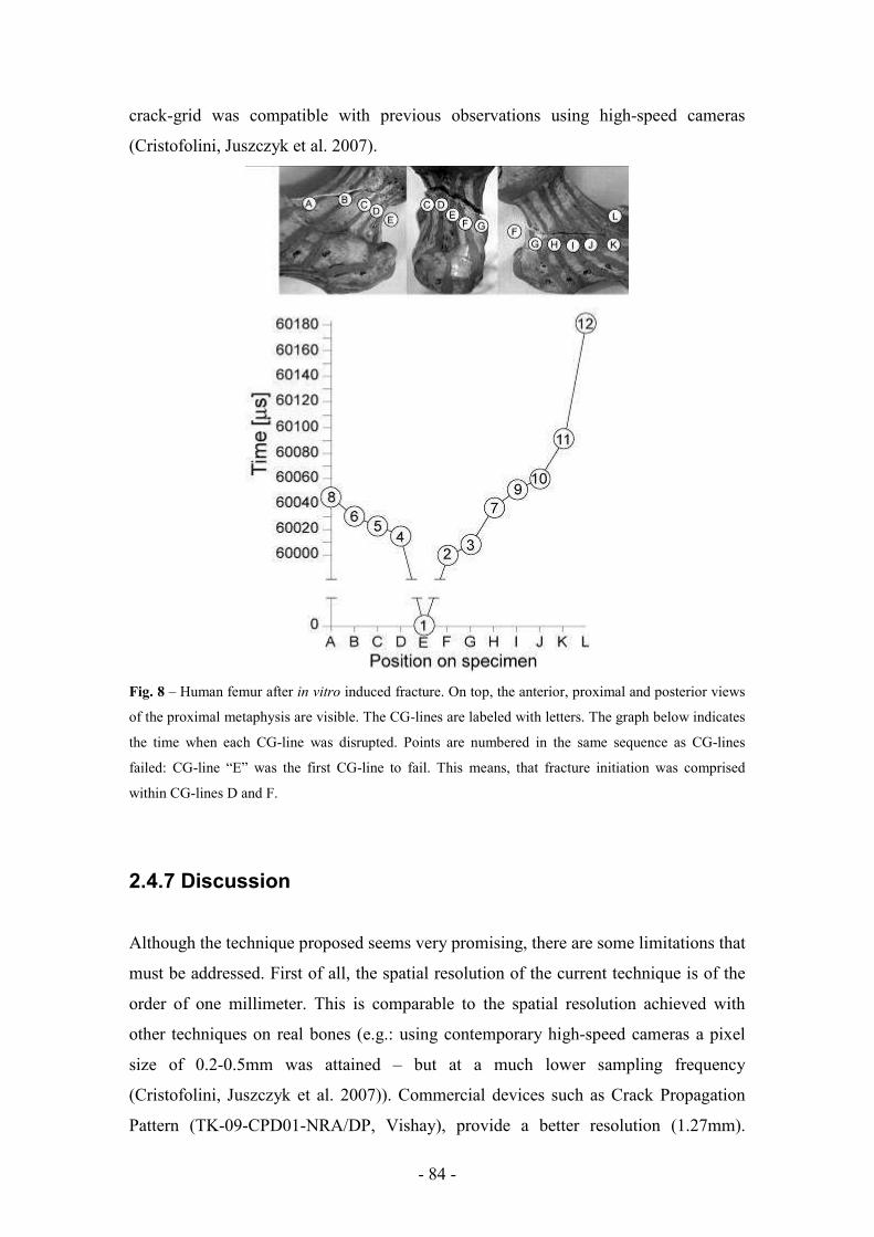
- 84 -
crack-grid was compatible with previous observations using high-speed cameras
(Cristofolini, Juszczyk et al. 2007).
Fig. 8 – Human femur after in vitro induced fracture. On top, the anterior, proximal and posterior views
of the proximal metaphysis are visible. The CG-lines are labeled with letters. The graph below indicates
the time when each CG-line was disrupted. Points are numbered in the same sequence as CG-lines
failed: CG-line “E” was the first CG-line to fail. This means, that fracture initiation was comprised
within CG-lines D and F.
2.4.7 Discussion
Although the technique proposed seems very promising, there are some limitations that
must be addressed. First of all, the spatial resolution of the current technique is of the
order of one millimeter. This is comparable to the spatial resolution achieved with
other techniques on real bones (e.g.: using contemporary high-speed cameras a pixel
size of 0.2-0.5mm was attained – but at a much lower sampling frequency
(Cristofolini, Juszczyk et al. 2007)). Commercial devices such as Crack Propagation
Pattern (TK-09-CPD01-NRA/DP, Vishay), provide a better resolution (1.27mm).

- 85 -
However, while this CG can only be applied to flat surfaces, the proposed crack-grid
can be applied to any geometry, including double-curvature surfaces of bones. It is
possible that with some more technical effort the spatial resolution of the proposed
crack-grid can be brought down to 0.5mm.
Secondly, the current sampling frequency (700kHz) is relatively high (state-of-the-.art
high-speed movies do not exceed 15kHz in these applications (Cristofolini, Juszczyk et
al. 2007)). A frequency of 700kHz is obviously much faster than most mechanical
events. The current version was based on inexpensive components. If, for some reason,
this scanning frequency is not sufficient, a faster system can be assembled based on
more performing electronics.
Third, it is important to remember that the ECD material was not originally designed
for this type of application. While extensive validation was carried out for monotonic
loading, the properties of this ECD material for a cyclic load have not been
characterized.
Fourth, preparation of the CG-lines requires a significant amount of manual work. The
entire process for preparing a crack-grid on the bone specimens described above
involved approximately 2 hours of a skilled operator. This obviously represents a cost.
This is also a source of variation if more specimens are to be prepared. It is worth
remarking that when bones are investigated, the irregular anatomy makes it necessary
in all cases to acquire the actual position of the constraints, sensors etc using a
digitizer. Therefore, this does not necessarily represent a problem. On the other hand,
the manual preparation of the crack-grid enables adapting the geometry of the crack-
grid to each specimen, considering anatomical details, surface defects and possible
regions of high interest.
Acknowledgments
The Authors wish to thank Lorenzo Zani for the technical support; Luigi Lena for the
artwork.
Conflict of interest statement
There is no potential conflict of interest: none of the Authors received or will receive
direct or indirect benefits from third parties for the performance of this study. Istituto
Ortopedico Rizzoli was partially funded by the European Community for the
performance of this study (project number: IST-2004-026932; title: Living Human
Digital Library; acronym: LHDL).

- 86 -
2.4.8 References
Amstutz, H. C., P. A. Campbell, et al. (2004). "Fracture of the neck of the femur after surface arthroplasty of the hip." J. Bone Jt. Surg. Am. 86: 1874-1877.
Bayraktar, H. H., E. F. Morgan, et al. (2004). "Comparison of the elastic and yield properties of human femoral trabecular and cortical bone tissue." J Biomech 37(1): 27-35.
Behiri, J. C. and W. Bonfield (1989). "Orientation dependence of the fracture mechanics of cortical bone." J Biomech 22(8-9): 863-72.
Bessho, M., I. Ohnishi, et al. (2007). "Prediction of strength and strain of the proximal femur by a CT-based finite element method." J Biomech 40(8): 1745-53.
Boudet, J. F., S. Ciliberto, et al. (1996). "Dynamics of Crack Propagation in Brittle Materials." J Phys 6(10): 1493-1516.
Cody, D. D., F. J. Hou, et al. (2000). "Short term in vivo precision of proximal femoral finite element modeling." Ann Biomed Eng 28(4): 408-14.
Crawford, R. P., C. E. Cann, et al. (2003). "Finite element models predict in vitro vertebral body compressive strength better than quantitative computed tomography." Bone 33(4): 744-50.
Cristofolini, L., M. Juszczyk, et al. (2007). "In vitro replication of spontaneous fractures of the proximal human femur." Journal of Biomechanics 40(13): 2837-2845.
Cristofolini, L., M. Juszczyk, et al. (IN PRESS 2009). "Strain distribution in the proximal human femoral metaphysis." Proc Inst Mech Eng [H] 223.
Currey, J. D. (2001). "Bone Strength: What are We Trying to Measure?" Calcified Tissue International 68(4): 205-210.
Fung, Y. C. (1980). Bone and cartilage. Biomechanics - Mechanical properties of living tissues. New York, Springer Verlag: 383-415.
Guyer, E. P. and R. H. Dauskardt (2004). "Electrical technique for monitoring crack growth in thin-film fracture mechanics specimens." J. Mater. Res.
Hansen, U., P. Zioupos, et al. (2008). "The effect of strain rate on the mechanical properties of human cortical bone." J Biomech Eng 130(1): 011011.
Hatakeyama, R., M. Yoshizawa, et al. "A Method for the Measurement of Acoustic Impedance and Speed of Sound in a Small Region of Bone using a Fused Quartz Rod as a Transmission Line." Japanese Journal of Applied Physics 39(Part 1, No. 11): 6449.
Jeffery, C. C. (1974). "Spontaneous fractures of the femoral neck." Orthop Clin North Am 5(4): 713-727.
Kanis, J. A., A. Oden, et al. (2007). "The use of clinical risk factors enhances the performance of BMD in the prediction of hip and osteoporotic fractures in men and women." Osteoporos Int 18(8): 1033-46.
Keaveny, T. M., P. F. Hoffmann, et al. (2008). "Femoral bone strength and its relation to cortical and trabecular changes after treatment with PTH, alendronate, and their combination as assessed by finite element analysis of quantitative CT scans." J Bone Miner Res 23(12): 1974-82.

- 87 -
Lee, T. C., S. Mohsin, et al. (2003). "Detecting microdamage in bone." J Anat 203(2): 161-72.
Malik, C. L., J. C. Gibeling, et al. (2002). "Compliance calibration for fracture testing of equine cortical bone." J Biomech 35(5): 701-5.
Malik, C. L., S. M. Stover, et al. (2003). "Equine cortical bone exhibits rising R-curve fracture mechanics." J Biomech 36(2): 191-8.
Murray, D. W., J. P. Little, et al. (2007). Femoral neck fractures following resurfacing. IMechE Conference: Engineers & Surgeons: joined at the hip, London, Institutions of Mechanical Engineers.
Nalla, R. K., J. S. Stölken, et al. (2005). "Fracture in human cortical bone: local fracture criteria and toughening mechanisms." Journal of Biomechanics 38(7): 1517-1525.
Norman, T. L., D. Vashishth, et al. (1992). "Effect of groove on bone fracture toughness." J Biomech 25(12): 1489-92.
Norman, T. L., D. Vashishth, et al. (1995). "Fracture toughness of human bone under tension." J Biomech 28(3): 309-20.
Prendergast, P. J. and D. Taylor (1994). "Prediction of bone adaptation using damage accumulation." J Biomech 27(8): 1067-76.
Ritchie, R. O., J. H. Kinney, et al. (2006). Cortical Bone Fracture. Wiley Encyclopedia of Biomedical Engineering. e. Metin Akay.
Rockwood, C. A. J., D. P. Green, et al. (1991). Rockwood and Green's fractures in adults. Philadelphia, J.B. Lippincott.
Rüedi, T. P. and W. M. Murphy (2001). AO principles of fracture management. Stuttgart, Georg Thieme Verlag.
Schileo, E., F. Taddei, et al. (2008). "Subject-specific finite element models implementing a maximum principal strain criterion are able to estimate failure risk and fracture location on human femurs tested in vitro." J Biomech 41(2): 356-67.
Schileo, E., F. Taddei, et al. (2007). "Subject-specific finite element models can accurately predict strain levels in long bones." J Biomech 40(13): 2982-9.
Shimmin, A. J. and D. Back (2005). "Femoral neck fractures following Birmingham hip resurfacing. A national review of 50 cases." J Bone Joint Surg Br. 87-B(3): 463-464.
Smirnov, V. (1968). "A method of measuring the crack propagation velocity in a rock specimen under impact load." Journal of Mining Science 4(3): 260-263.
Spierings, A. B. and S. Derler (2005). "Assessment of hip protectors and corresponding hip fracture risk using stress calculation in the femoral neck." Med. Eng. Phys. IN PRESS: IN PRESS.
Thurner, P. J., B. Erickson, et al. (2006). "High-speed photography of the development of microdamage in trabecular bone during compression." J Mater Res 21(5): 1093-1100
Vashishth, D., J. C. Behiri, et al. (1997). "Crack growth resistance in cortical bone: concept of microcrack toughening." J Biomech 30(8): 763-9.

- 88 -
WHO (1994). Assessment of fracture risk and its application to screening for postmenopausal osteoporosis. Report of a WHO study group. WHO Technical Report Series, World Health Organization, Geneva, Switzerland, 843: 1-130.
Wilkin, T. J. and D. Devendra (2001). "Bone densitometry is not a good predictor of hip fracture." Bmj 323(7316): 795-7.
Yang, Q. D., B. N. Cox, et al. (2006). "Fracture length scales in human cortical bone: the necessity of nonlinear fracture models." Biomaterials 27(9): 2095-113.
Yao, X., P. Wang, et al. (2008). "Experimental study of damage and fracture of cancellous bone using a digital speckle correlation method." J Biomed Opt 13(3): 034026.

- 89 -
3 GENERAL BIOMECHANICAL CHARACTERIZATION OF LONG BONES

- 90 -
3.1 LHDL related data acquisition The Living Human Digital Library research project involved a massive data collection
activity, aimed to the creation of the most detailed single-subject collection on
biomechanical and anatomo-functional data of the musculoskeletal system. The
various methods used in this huge endeavour were documented in detail in a collection
of brief technical notes that are now publicly available.
This chapter summaries work done so far at the organ level. Brief description of type
of data collected; procedures for handling specimens and data acquisition and list of
bone segments tested, is given here.
The detailed description of the methods used for the data collection, is progressively
shared by the involved institutions with the rest of the worldwide research community
through the Physiome Space service that emerged from the LHDL project.
(www.livinghuman.org , www.biomedtown.org)
Six human long bone segments underwent biomechanical mechanical investigation. Each one was tested in elastic and to failure range with respect to the physiologically most relevant ways (see Table1). Table 1 Test performed on each bone segment
BONE SEGMENT
NON DISTRUCTIVE TESTING
TEST TO FAILURE
RADIUS 4PB /
TORSION 4PB
ULNA 4PB /
TORSION 4PB
HUMERUS 4PB /
TORSION TORSION
FEMUR 4PB /
TORSION SPECIFIC STUDY ON PROSIMAL
METAPHYSIS
TIBIA 4PB /
TORSION
SPECIFIC STUDY OVER PHISIOLOGICAL FUNCTION AND ANATOMICAL
MORPHOLOGY
FIBULA 4PB /
TORSION 4PB

- 91 -
3.1.1 Whole-bone stiffness
Specimens: The following long bones were fully characterized to assess the whole-
bone stiffness: femur, tibia, fibula, first to fifth metatarsal bones. Both right and left
limb from the first donor were examined.
Loading configurations: The following loading scenarios were applied:
• Four point bending: the diaphysis was bent by using a four roller configuration
in the following directions (Figure 1):
o Sagittal plane, causing tension on the anterior side
o Sagittal plane, causing tension on the posterior side
o Frontal plane, causing tension on the medial side
o Frontal plane, causing tension on the lateral side
Fig 1. Four point bending of the tibia.
• Torsion about the long axis of the diaphysis was applied by means of pots that
clamped the bone extremities:
o Torque towards intra-rotation of the foot
o Torque towards extra-rotation of the foot
• In addition, the femur underwent six additional load cases were the femur was
tilted by different angles with respect to the vertical while a force was applied

- 92 -
to the femoral head. A constraint was applied lo that only the proximal third of
the femur was exposed to load.
Measured quantities: Stiffness test consisted in applying loading while deflection was
measured by means of high precision displacement transducers.
Applied loads: To prevent tissue damage due to repeated loading, a load equal to 10%
of the estimated failure load was applied for each loading configuration.
Loading rate: Load was applied at two loading rates. The highest loading rate was
calculated so as to induce a strain rate that would bring the bone to failure in 0.1-0.3
seconds. The lowest loading rate was 10 times lower.
Repetitions: each non destructive loading scenario and loading rate was applied 5
times on each bone
3.1.2 Strain distribution in whole bones
While the whole-bone stiffness was assessed, strain on the bone surface was measured.
Strain was measured for all the loading scenarios indicated above.
Strain measurement: triaxial stacked strain rosettes were used. This type of transducer
allows measuring all components of surface strain and their direction, even in regions
with high strain gradients. Suitable procedures were used to bond the strain gauges to
the bone surface without compromising tissue preservation or sensor insulation (Fig
2).
Fig 2. Tibia with triaxial rosettes.

- 93 -
Strain measurement locations: the position of the strain gauges was designed so as to
enable sampling the strain distribution in the most relevant regions. The different
bones were mapped as follows:
• Femur (four point bending and torsion tests): 12 strain gauges placed around
the diaphysis at 3 equally spaced levels
• Femur (six loading directions on the femoral head): 13 strain gauges placed
around the head, neck and diaphysis at 3 levels
• Tibia (four point bending and torsion tests): 15 strain gauges placed around the
diaphysis at 4 equally spaced levels
• Fibula (four point bending and torsion tests): 8 strain gauges placed around the
diaphysis at 4 equally spaced levels
3.1.3 Whole-bone strength
After completion of the stiffness and strain measurement, bone strength was assessed
by applying a load ramp until specimen failed.
Loading configurations: The following loading scenarios were applied:
• Femur: load on the femoral head (8° in the frontal plane)
• Tibia: four point bending
• Fibula: four point bending
• Metatarsal bones: torsion
Measured quantities: Load and displacement were acquired during the test, together
with strain from the strain gauges (sampling rate 2kHz). High speed videos (10000
frames per second) were recorded for selected specimens to identify the point of
fracture initiation. Selected specimens were instrumented with a dedicated proprietary
sensor to identify the point of fracture initiation.
Loading rate: Load was applied at the highest loading rate used in the stiffness
measurement tests.

- 94 -
This was calculated so as to induce a strain rate that would bring the bone to failure in
0.1-0.3 seconds.
Repetitions: because of the destructive nature of these tests, each specimen could be
tested only once.

- 95 -
3.2 STRUCTURAL BEHAVIOUR OF THE LONG BONES OF THE HUMAN LOWER LIMBS
Luca Cristofolini, PhD 1, 2, Giorgia Conti, MEng 1, 2, Mateusz Juszczyk, MEng 1, 2, PhD 1, Sara Cremonini MSc 1, Marco Viceconti, PhD 1
1 Laboratorio di Tecnologia Medica, Istituto Ortopedico Rizzoli, Bologna, Italy 2 Engineering Faculty, University of Bologna, Italy
Submitted: J. Biomechanics

- 96 -
3.2.1 INTRODUCTION
Aim of the present study was:
• Assess the stiffness and strain distributions of the different low limb bones from the
same donors;
• Assess if there is any significant effect of viscoelasticity on the strain values within a
physiological range of strain rates;
• Assess if the structure and the material properties cause any difference in the behavior
in relation to the direction of the applied load, especially considering opposite directions
of bending and torsion.
3.2.2 MATERIALS AND METHODS
3.2.2.1 Design of the experiment
The structural stiffness and strain distribution of the long bones of the lower limb were
assessed: the proximal metaphysis and the diaphysis of the femur, and the diaphysis of the
tibia and fibula were investigated.
3.2.2.2 Specimens
Bone specimens were obtained from two donors who did not suffer from cancer nor
musculoskeletal diseases (Table 1). Bone specimens were embalmed following a validated
procedure (Ohman, Dall'Ara et al. 2008). Tissue hydration was constantly preserved using
moistened cloths. All bone segments (12 in total) were inspected and CT-scanned to
exclude fractures or any other defect. Anatomical reference frames were marked on each
bone ((Ruff and Hayes 1983; Cristofolini 1997) for the femur; (Conti, Cristofolini et al.
2008) for the tibia and fibula). Anatomical dimensions were measured according to ((Ruff
and Hayes 1983), Table 1).
Table 1 – In the first columns the details of the donors are reported. In the following columns the anatomical
details of the bone specimens analyzed are reported. The diameter of the head of the femur was measured five
times along different directions; the average head diameter, HD, was computed as in (Cristofolini, Juszczyk et
al. IN PRESS). The ‘biomechanical length’ of the femur (BLF, see also Fig. 2) was defined as in (Ruff and

- 97 -
Hayes 1983); the ‘biomechanical length’ of the tibia and fibula (BLT, see also Fig. 3) was defined as in
(Conti, Cristofolini et al. 2008).
FEMUR TIBIA AND FIBULA
Head Diameter, HD
(mm)
Biomechanical Length, BLF (mm)
Biomechanical Length, BLT (mm)
Age at death (years)
Donors' height (cm)
Donors' Body Weight, BW (kg)
Body Mass Index, BMI
(kg/m2) Gender
Right Left Right Left Right Left
Donor #1 72 165 63 23.1 female 47.5 47.5 427 427 362 364
Donor #2 72 171 64 21.9 female 46.5 47.8 415 412 351 346
3.2.2.3 Strain measurement
Each bone segment was instrumented with triaxial-stacked strain gauges following a
validated procedure (Viceconti, Toni et al. 1992; Cristofolini, Juszczyk et al. IN PRESS):
• Proximal femoral metaphysis: 16 strain gauges (KFG-1-120-D17-23L3M2S, Kyowa,
Tokyo, Japan, grid length=1mm) (Fig. 1) (Cristofolini, Juszczyk et al. IN PRESS);
• Femoral diaphysis: 16 strain gauges (KFW-2-350-D17-23L2M2S, Kyowa, grid
length=2mm) (Fig. 2);
• Tibial diaphysis: 15 strain gauges (KFW-2-350-D17-23L2M2S, Kyowa, grid
length=2mm) (Fig. 3);
• Fibular diaphysis: 8 strain gauges (KFG-1-120-D17-23L3M2S, Kyowa, grid
length=1mm) (Fig. 4).

- 98 -
Fig. 1 – Anterior and lateral views of the proximal metaphysis of a right femur. The position of the strain
gauges is reported: 4 around the head, close to the articular cartilage (AH, LH, PH, MH); 4 around the neck,
distal to the previous ones (AN, LN, PN, MN); 4 around the proximal diaphysis, just below the lesser
trochanter (A0, L0, P0, M0); 4 around the proximal part of diaphysis (A1, L1, P1, M1: they were the same as
in the femoral diaphysis, Fig. 2). To enable scaling between specimens, all lengths were defined as a fraction
of the head diameter (HD) or of the biomechanical length of the femur (BLF). The femur was held distally
using a pot made of acrylic bone cement (a). The pot could be tilted so that the hip joint resultant force (F)
was applied at the prescribed angles in the frontal plane (α), and in the sagittal plane (β), as in (Cristofolini,
Juszczyk et al. IN PRESS).

- 99 -
Fig. 2 – Anterior and lateral views of a right femur. The position of the strain gauges is reported: 4 at each of
4 levels, on the Anterior, Lateral, Medial and Posterior sides (gauges A1, L1, P1, M1 were the same as in the
proximal femoral metaphysis, Fig. 1). To enable scaling between specimens, all lengths were defined as a
fraction of the biomechanical length of the femur (BLF). The torsional load was applied by means of proximal
(a) and distal (b) pots made of acrylic bone cement. Also indicated is the position of the rollers to apply four-
point-bending in the different directions (Table 2): rollers (LM) acted in a frontal plane generating tension on
the medial side; rollers (ML) generated tension on the lateral side; rollers (PA) acted in a sagittal plane
generating tension on the anterior side; rollers (AP) generated tension on the posterior side. The most
proximal rollers always rested on the flat faces of pot (a) to prevent the specimen from rotating axially.

- 100 -
Fig. 3 – Anterior and lateral views of a right tibia. The position of the strain gauges is reported: 4 at each of 4
levels, on the Anterior, Lateral, Medial and Posterior sides (only the most distal level had 3 gauges: M4 was
not installed). To enable scaling between specimens, all lengths were defined as a fraction of the
biomechanical length of the tibia (BLT). The torsional load was applied by means of a proximal (a) and a
distal (b) pot made of acrylic bone cement. Also indicated is the position of the rollers to apply four-point-
bending in the different directions (Table 2): rollers (LM) acted in a frontal plane generating tension on the
medial side; rollers (ML) generated tension on the lateral side; rollers (PA) acted in a sagittal plane generating
tension on the anterior side; rollers (AP) generated tension on the posterior side. The most proximal rollers
always rested on the flat faces of pot (g) to prevent the specimen from rotating axially.

- 101 -
Fig. 4 – Anterior and lateral views of a right fibula. The position of the strain gauges is reported: 2 at each of 4
levels (either Anterior and Posterior, or Lateral and Medial). To enable scaling between specimens, all lengths
were defined as a fraction of the biomechanical length (BLT). The torsional load was applied by means of a
proximal (a) and a distal (b) pot made of acrylic bone cement. Also indicated is the position of the rollers to
apply four-point-bending in the different directions (Table 2): rollers (LM) acted in a frontal plane generating
tension on the medial side; rollers (ML) generated tension on the lateral side; rollers (PA) acted in a sagittal
plane generating tension on the anterior side; rollers (AP) generated tension on the posterior side. The most
proximal rollers always rested on the flat faces of pot (a) to prevent the specimen from rotating axially.
A grid excitation of 0.5V was selected to avoid heating. Strains and load-displacement data
from the testing machine were sampled at 2000Hz, using a 50-channel data logger (System-
6000, Vishay Micro-Measurement, USA). Principal strains (ε1 and ε2) were computed based
on the three grids of each strain gauge.
3.2.2.4 In vitro loading
All specimens were tested using an axial-torsional servo-hydraulic machine (858-
MiniBionix, MTS, Minneapolis, USA). For each type of loading, suitable loading setups
were designed (using hinges and universal joints) that avoided any additional load
components.

- 102 -
To investigate the strain distribution in the proximal metaphysis, a single force was applied
to the femoral head at different directions, simulating the hip joint resultant force during
daily loading (Fig. 1 (Cristofolini, Juszczyk et al. IN PRESS)). Muscle forces were not
simulated, as they do not significantly alter the stress distribution in the proximal
metaphysis (Cristofolini, Viceconti et al. 1995; Cody, Gross et al. 1999; Keyak, Kaneko et
al. 2005; Taddei, Cristofolini et al. 2006; Cristofolini, Juszczyk et al. 2007). Four
configurations were designed to cover the physiological range of loading directions during a
variety of activities (Bergmann, Deuretzbacher et al. 2001). The cone spanned by the hip
joint resultant force was calculated: LC1-LC4 (Table 2) corresponded to the extreme angles
of the resultant force in the frontal and sagittal planes (Taddei, Cristofolini et al. 2006). To
replicate a loading configuration used in the literature to replicate simplified single-leg
stance, the hip joint resultant force was applied parallel to the femoral diaphysis (LC5 in
Table 2). The last configuration (LC6 in Table 2) has been proposed to in vitro replicate
spontaneous fractures of the proximal femur (i.e. not associated with any primary trauma,
but due to sudden application of para-physiological load peaks, e.g. while mis-stepping or
stumbling) (Cristofolini, Juszczyk et al. 2007).
The procedure for four-point-bending of the diaphysis of the femur, tibia and fibula was
consistent with (Cristofolini, Viceconti et al. 1996; Cristofolini and Viceconti 2000; Heiner
and Brown 2001; Gray, Taddei et al. 2008): equally spaced rollers generated bending either
in the frontal plane and sagittal plane (Figs.2-4). Deflection at the mid-point was measured
by a single-arm Extensometer (632.06H-20, MTS, Minneapolis, USA). Bending in each
plane was exerted in both opposite direction to assess if a difference existed (Table 2).
Bending stiffness was defined as the average slope of the load-deflection curve between
10% and 90% of the full load.
The procedure for torsional testing of the diaphysis of the femur, tibia and fibula was
consistent with (Cristofolini, Viceconti et al. 1996; Cristofolini and Viceconti 2000; Heiner
and Brown 2001; Gray, Taddei et al. 2008): rotation was recorded while the testing machine
applied a controlled torque to the extremities of the diaphysis. Torsion was exerted in both
opposite direction to assess if a difference existed (Table 2). Torsional stiffness was defined
as the average slope of the torque-rotation curve between 10% and 90% of the full load.
To avoid risk of damage during testing, the failure load for each configuration was
estimated with preliminary Finite Element models, using a validated procedure (Schileo,

- 103 -
Taddei et al. 2007; Schileo, Taddei et al. 2008). The applied load was 10% of the estimated
failure load.
To cover the range of physiological strain rates, load was applied at two different speeds:
• High-strain-rate: the load ramp was tuned so that the strain rate in the most stressed
regions was 0.05s-1. As bone tissue fails when strain exceeds 0.007-0.01(Bayraktar,
Morgan et al. 2004), such strain rate would generate failure in the order of 0.2seconds.
This is the typical timescale of physiological and para-physiological loading
(Bergmann, Deuretzbacher et al. 2001; Bergmann, Graichen et al. 2004).
• Low-strain-rate: a strain rate ten times lower than high-strain-rate was implemented to
replicate quasi-static loading events;
• For both strain rates, the maximum load was held for 2seconds before unloading.
Each loading configuration was tested six times on each specimen, dismounting and
realigning the entire loading setup between repetitions. Bone specimens were allowed to
recover at least 3minutes between repetitions.
3.2.5 Statistical analysis
Linearity between force and strain was checked by linear regression separately for each
strain gauge and each specimen.
To assess the effect of the loading direction and loading rate on the stiffness of the bones, a
Factorial ANOVA (with Scheffe post-hoc test) was performed separately for the two donors
and for each bone segment (femur, tibia, fibula). A power analysis was performed for
statistically non-significant effects. The following independent factors were examined:
• Donor’s side (right, left)
• Loading configuration (6 configurations for the proximal metaphysis, 4 for four-point-
bending, 2 for torsion);
• Test speed (high-strain-rate, low-strain-rate).
A similar analysis was performed also on the strain distribution, where the strain
measurement location was included as an additional factor.
To assess the effect of opposite directions of loading (e.g. intra-rotations vs. extra- rotation)
on the strain distribution, the correlation between the strain measured with opposite
directions of applied load was investigated by means of linear regression.

- 104 -
To assess the effect of the loading rate on the strain distribution, the correlation between the
strain measured at high-strain-rate and low-strain-rate was investigated by means of linear
regression.
All statistical analyses were performed using dedicated software (StatView-5.0.1, SAS-
Institute, Cary, NC, USA, and SPSS-16.0, SPSS Inc., Chicago, IL, USA).
3.2.3 RESULTS
3.2.3.1 Linearity and creep
Linearity between load and displacement was excellent (R2≥0.98). Also load-strain and
displacement-strain linearity was excellent (R2≥0.97 where strain exceeded 100
microstrain).
Strain magnitude tended to increase over time by typically 0.1-3.0% of the initial value
while load was held (for 2 seconds). After unloading, strain returned rapidly to zero, with
residual strain (3 minutes after unloading) of 0.5%-4% percent of the peak value.
Strain measurement repeatability (intra-specimen variability) was good: the Coefficient of
Variation (CoV) between replicates under the same conditions was on average 0.4% for the
proximal femoral metaphysis, 2.5% for four-point-bending, and 0.5% for torsion.
3.3.3.2 Stiffness and strain distribution
The right specimen was generally stiffer than the controlateral one both in bending and in
torsion for both donors (Figs. 5-7; Factorial ANOVA, p<0.001). The only exception was the
bending stiffness of the femoral diaphysis: the difference between controlateral specimens
was not significant, for both donors (Factorial ANOVA, p>0.1, power=0.4).

- 105 -
Fig. 5 – Stiffness of the diaphysis of the femur for the right and left specimens of donors #1 and #2 (average ±
standard deviation between 6 test repetitions), and on average (average ± standard deviation between 4
specimens). Bending stiffness was measured as in a sagittal plane, with tension on the posterior (AP) and
anterior side (PA), and in a frontal plane, with tension on the lateral (ML) and medial side (LM). Torsional
stiffness was measured applying intra-rotation (Intra) and extra-rotation (Extra) of the distal extremity. Data
represented here correspond to the low-strain-rate; similar trends were observed for the high-strain-rate.
Fig. 6 – Stiffness of the diaphysis of the tibia for the right and left specimens of donors #1 and #2 (average ±
standard deviation between 6 test repetitions), and on average (average ± standard deviation between 4
specimens). Bending stiffness was measured as in a sagittal plane, with tension on the posterior (AP) and
anterior side (PA), and in a frontal plane, with tension on the lateral (ML) and medial side (LM). Torsional
stiffness was measured applying intra-rotation (Intra) and extra-rotation (Extra) of the distal extremity. Data
represented here correspond to the low-strain-rate; similar trends were observed for the high-strain-rate.

- 106 -
Fig. 7 – Stiffness of the diaphysis of the fibula for the right and left specimens of donors #1 and #2 (average ±
standard deviation between 6 test repetitions), and on average (average ± standard deviation between 4
specimens). Bending stiffness was measured as in a sagittal plane, with tension on the posterior (AP) and
anterior side (PA), and in a frontal plane, with tension on the lateral (ML) and medial side (LM). Torsional
stiffness was measured applying intra-rotation (Intra) and extra-rotation (Extra) of the distal extremity. Data
represented here correspond to the low-strain-rate; similar trends were observed for the high-strain-rate.
Similarly, the strain distribution differed significantly between controlateral specimens
(Factorial ANOVA, p<0.0005, for the femur, tibia and fibula). Also significant was the
difference between strains measured at different locations (Factorial ANOVA, p<0.0005, in
all bone segments). For space reasons, more details about the strain distribution are not
reported on web site dedicated LHDL project.
3.2.3.3 Effect of loading rate
Most bones were slightly stiffer at high-strain-rate than at low-strain-rate, although this
difference was not always significant (Table 3). Slightly lower strain values were found at
high-strain-rate for the proximal metaphysis and diaphysis of the femur for all loading
configurations, while this difference was not significant in the tibia and fibula (Table 3, Fig.
8).
Table 2 – Details of the loading configurations applied to the femur, tibia and fibula: direction and magnitude
of applied loads.
DIRECTION OF APPLIED LOAD FEMUR TIBIA FIBULA
PROXIMAL METAPHYSIS
Direction of applied force (α and βdefined in Fig. 1):
LC1:Max flexion: α=0°, β=+18° LC2: Max abduction: α=+3°, β=0° LC3: Max extension: α=0°, β=-3° LC4: Max adduction : α=+24°, β=0° LC5: Neutral: α=0°, β=0°
Magnitude of applied force:
0.75BW
N.A.
N.A.

- 107 -
LC6: Simulated failure: α=+8°, β=0°
FOUR-POINT-BENDING
Direction of applied flexion:
AP: bending in sagittal plane (tension on posterior side) PA bending in sagittal plane (tension on anterior side) ML: bending in frontal plane (tension on lateral side) LM: bending in frontal plane (tension on medial side)
Magnitude of applied force at each roller: 0.563 BW
Magnitude of applied force at each roller: 0.243 BW
Magnitude of applied force at each roller: 0.0324 BW
TORSION
Direction of applied torque: INTRA: torque causing intra-rotation of the distal extremity EXTRA: torque causing extra-rotation of the distal extremity
Magnitude of applied torque:
42.1 BW*mm
Magnitude of applied torque:
11.9 BW*mm
Magnitude of applied torque:
0.985BW*mm
Fig. 8 – Correlation between strain at low-strain-rate and high-strain-rate for the proximal metaphysis of the
femur (a), the diaphysis of the femur (b), tibia (c) and fibula (d). All specimens (right and left from both
donors), all loading configurations and all strain measurement locations are pooled. A slope equal to 1.000
would indicate that identical strain values are obtained at both strain rates; a slope lower than 1.000 indicates
that strains are lower when a higher strain rate is applied.

- 108 -
3.2.3.4 Effect of loading direction
The direction of the applied load had a significant effect on the bending stiffness (factorial
ANOVA, p<0.0005, Figs. 5-7). The femur was stiffer in the frontal than in the sagittal plane
(Scheffe test, p<0.0005). The tibia and fibula were stiffer in the sagittal than in the frontal
plane (Scheffe test, p<0.0005). Remarkably, differences existed also between bending in
opposite directions in the same plane (Table 3). Similarly, the direction of the applied
torque (intra-rotation vs extra-rotation) had a significant effect on the stiffness (Factorial
ANOVA, p<0.0005 for all bone segments, Figs. 5-7).
Table 3 – In the first part (three rows), the significance of the loading rate is reported for the structural stiffness and for the strain distribution. In the last part, the significance of the differences between specific load configurations is reported: opposite directions of loading are compared for the stiffness and for the strain distribution. Significance is expressed in terms of Scheffe post-hoc p-value.
FEMUR TIBIA FIBULA
Proximal
metaphysis
Slightly lower strain at high-strain-rate (p<0.1)
N.A.
N.A.
Diaphysis: four-point-bending
Similar stiffness at high-and low-strain-rate
(p>0.2) Lower strain at high-strain-rate (p<0.05)
Similar stiffness at high-
and low-strain-rate (p>0.2)
Similar strain at both strain rates (p>0.1)
16% Stiffer at high-strain-rate (p<0.005)
Similar strain at both strain rates (p>0.1)
Effect of
loading rate
Diaphysis: torsion
4% Stiffer at high-strain-
rate (p<0.005)
Lower strain at high-strain-rate (p<0.005)
6% Stiffer at high-strain-
rate (p<0.05)
Similar strain at both strain rates (p>0.1)
Similar stiffness at high-and low-strain-
rate (p>0.2)
Similar strain at both strain rates (p>0.1)
Diaphysis: four-point-bending in sagittal plane
Stiffer when anterior side was in tension
(p<0.0005)
Different strain distribution for opposite directions of bending
(p<0.0005)
Stiffer when posterior side was in tension (p<0.0005)
Different strain distribution for opposite directions of
bending (p<0.0005)
Stiffer when posterior side was in tension
(p<0.05)
Different strain distribution for
opposite directions of bending (p<0.0005)
Diaphysis: four-point-bending in frontal plane
Stiffer when lateral side
was in tension (p<0.0005)
Different strain
distribution for opposite directions of bending
(p<0.0005)
Stiffer when medial side was in tension (p<0.02)
Different strain distribution for opposite directions of
bending (p<0.0005)
Stiffer when medial side was in tension
(p<0.002)
Different strain distribution for
opposite directions of bending (p<0.0005)
Effect of
opposite
directions of
applied load
Diaphysis: torsion
Stiffer in intra-rotation than extra-rotation
(p<0.0005)
Similar strain distribution for opposite directions of
torsion (p>0.5, power>0.8)
Stiffer in extra-rotation than intra-rotation
(p<0.0005)
Different strain distribution for opposite directions of
torsion (p<0.0005)
Stiffer in extra-
rotation than intra-rotation (p<0.0005)
Similar strain distribution for
opposite directions of torsion (p>0.2)

- 109 -
Also the strain distribution was significantly affected by the direction of the applied load
(Factorial ANOVA, p<0.0005 for all bone segments). Such difference existed not only
between the most obvious configurations (e.g. bending in the frontal vs sagittal planes), but
also for opposite directions of loading (Table 3). As an example, the effects of opposite
directions of torsion are compared in Fig. 9.
Fig. 9 – Correlation between strain when a torque was applied in two opposite directions (intra-rotation vs
extra-rotation of the distal extremity). Strains are plotted separately for the diaphysis of the femur (a), tibia (b)
and fibula (c). All specimens (right and left from both donors), all loading configurations and all strain
measurement locations are pooled. A slope equal to one would indicate that identical strain values are
obtained for opposite loading directions; a slope lower than unity indicates that strains are lower when extra-
rotation is applied to the distal extremity. Data represented here correspond to the low-strain-rate (similar
results were obtained at high-strain-rate).
Acknowledgments The Authors wish to thank Caroline Öhman and Andrea Malandrino for their support in
digitizing the landmarks, Keith Smith for revising the script, and Luigi Lena for the
artwork. This work was partially supported by the European Community (project number:
IST-2004-026932; title: Living Human Digital Library; acronym: LHDL)

- 110 -
3.2.4 References
Bayraktar, H. H., E. F. Morgan, et al. (2004). "Comparison of the elastic and yield properties of human femoral trabecular and cortical bone tissue." J Biomech 37(1): 27-35.
Bergmann, G., G. Deuretzbacher, et al. (2001). "Hip contact forces and gait patterns from routine activities." J Biomech 34(7): 859-71.
Bergmann, G., F. Graichen, et al. (2004). "Hip contact forces during stumbling." Langenbecks Arch. Surg. 389: 51-59.
Cody, D. D., G. J. Gross, et al. (1999). "Femoral strength is better predicted by finite element models than QCT and DXA." J Biomech 32(10): 1013-20.
Conti, G., L. Cristofolini, et al. (2008). "Comparison of three standard anatomical reference frames for the tibia-fibula complex." J Biomech 41(16): 3384-3389.
Cristofolini, L. (1997). "A critical analysis of stress shielding evaluation of hip prostheses." Critical Reviews in Biomedical Engineering 25:4&5: 409-483.
Cristofolini, L., M. Juszczyk, et al. (2007). "In vitro replication of spontaneous fractures of the proximal human femur." J. Biomechanics 40(13): 2837-2845.
Cristofolini, L., M. Juszczyk, et al. (IN PRESS). "Strain distribution in the proximal human femoral metaphysis." Proc Inst Mech Eng [H].
Cristofolini, L. and M. Viceconti (2000). "Mechanical validation of whole bone composite tibia models." J Biomech 33(3): 279-88.
Cristofolini, L., M. Viceconti, et al. (1996). "Mechanical validation of whole bone composite femur models." J Biomech 29(4): 525-35.
Cristofolini, L., M. Viceconti, et al. (1995). "Influence of thigh muscles on the axial strains in a proximal femur during early stance in gait." J Biomech 28(5): 617-624.
Gray, H. A., F. Taddei, et al. (2008). "Experimental validation of a finite element model of a human cadaveric tibia." J. Biomech. Engineering 130(3): 031016-1 (9 pages).
Heiner, A. D. and T. D. Brown (2001). "Structural properties of a new design of composite replicate femurs and tibias." J Biomech 34(6): 773-81.
Keyak, J. H., T. S. Kaneko, et al. (2005). "Predicting proximal femoral strength using structural engineering models." Clin Orthop Relat Res(437): 219-28.
Ohman, C., E. Dall'Ara, et al. (2008). "The effects of embalming using a 4% formalin solution on the compressive mechanical properties of human cortical bone." Clin Biomech (Bristol, Avon) 23(10): 1294-8.
Ruff, C. B. and W. C. Hayes (1983). "Cross-sectional Geometry of Pecos Pueblo Femora and Tibiae - A Biomechanical Investigation: I. Method and General Patterns of Variation." Am. J. Phys. Anthropol. 60: 359-381.
Schileo, E., F. Taddei, et al. (2008). "Subject-specific finite element models implementing a maximum principal strain criterion are able to estimate failure risk and fracture location on human femurs tested in vitro." J Biomech 41(2): 356-67.
Schileo, E., F. Taddei, et al. (2007). "Subject-specific finite element models can accurately predict strain levels in long bones." J Biomech 40(13): 2982-9.
Taddei, F., L. Cristofolini, et al. (2006). "Subject-specific finite element models of long bones: An in vitro evaluation of the overall accuracy." J Biomech 39(13): 2457-67.
Viceconti, M., A. Toni, et al. (1992). Strain gauge analysis of hard tissues: factors influencing measurements. Experimental Mechanics. Technology transfer between

- 111 -
high tech engineering and biomechanics. E. G. Little. Amsterdam, Elsevier Science Publisher B.V.: 177-184.

- 112 -
4.1 STRAIN DISTRIBUTION IN THE PROXIMAL HUMAN FEMORAL METAPHYSIS
Luca Cristofolini, Ph.D. 1, 2, Mateusz Juszczyk, M.Eng. 1,2, Fulvia Taddei, Ph.D. 1, Marco
Viceconti, Ph.D. 1
1 Laboratorio di Tecnologia Medica, Istituto Ortopedico Rizzoli, Bologna, Italy 2 Engineering Faculty, University of Bologna, Italy
This paper is in press on Proceedings of the Institution of Mechanical Engineers, PartH, Journal of Engineering in Medicine.

- 113 -
4.1.1 ABSTRACT
There is a significant interest in the state of stress/strain in the proximal femoral
metaphysis, because of its relevance for hip fractures and prosthetic replacements. The
scope of this work was to provide a better understanding of the strain distribution, and of its
correlation with the different directions of loading, and with bone quality. Twelve pairs of
human femurs were instrumented with strain gauges. Six loading configurations were
designed to cover the range of directions spanned by the hip joint force. Inter-specimen
variability was reduced if paired specimens were considered. Principal strain magnitude
varied greatly between loading configurations. This suggests that different loading
configurations need to be simulated in vitro. The strain magnitude varied between locations,
but on average was compatible with the strain values measured in vivo. The strain
magnitudes and the direction of principal tensile strain in the head and neck were
compatible with the spontaneous fractures of the proximal femur reported in some subjects.
Principal tensile strain was significantly larger where cortical bone was thinner;
compressive strain was larger where cortical bone was thicker. The direction of principal
strain varied significantly between measurement locations, but varied little between loading
configurations. This suggests that the anatomy and the distribution of anisotropic material
properties enable the proximal femur to adequately respond to the changing direction of
daily loading.
Keywords: proximal human femoral metaphysis; strain distribution; loading condition; paired and unpaired variability; direction of principal strain

- 114 -
List of abbreviations:
ε1 maximum principal strain
ε2 minimum principal strain
θp angle of the principal planes (counter-clockwise)
BW Body Weight
FE Finite Element
LC load configuration (six different configurations were tested: LC1-LC6)
AH strain gauge on the anterior side of the head
LH strain gauge on the lateral side of the head
PH strain gauge on the posterior side of the head
MH strain gauge on the medial side of the head
AN strain gauge on the anterior side of the neck
PN strain gauge on the posterior side of the neck
MN strain gauge on the medial side of the neck
A1 strain gauge on the anterior side, below the lesser trochanter
L1 strain gauge on the lateral side, below the lesser trochanter
P1 strain gauge on the posterior side, below the lesser trochanter
M1 strain gauge on the medial side, below the lesser trochanter

- 115 -
4.1.2 INTRODUCTION
Strain distribution in the proximal femur always had a great interest in biomechanics. The
recent resurgence of epiphyseal hip prostheses requires a deep understanding of the stress
distribution in the proximal femoral metaphysis, because of the potential risk of neck
fracture and adverse bone remodeling (Amstutz, Campbell et al. 2004; Grigoris, Roberts et
al. 2006; McMinn and Daniel 2006). Also, the increased rate of traumatic and spontaneous
fractures (i.e.: caused by sudden loading and muscle contraction, not by trauma) of the
proximal femur associated with the aging population (Grisso, Kelsey et al. 1991;
Rockwood, Green et al. 1991) suggests that more research should focus on the
biomechanics of such fractures, to improve the understanding of their etiology (Yang, Shen
et al. 1996; Cristofolini, Juszczyk et al. 2007). Recently, a multi-scale approach was taken
by many researchers to investigate musculoskeletal biomechanics in general (Fenner, Brook
et al. 2008), and especially focusing on the proximal femoral metaphysis (Cristofolini,
Taddei et al. 2008; Viceconti, Taddei et al. 2008): this approach requires quantitative
information about the strain distribution under load.
The stress/strain distribution in the femur has been extensively studied in the past (Fung
1980; Roesler 1987; Fabeck, Tolley et al. 2002). However, most of the published
experimental studies were designed to investigate the effect of hip stems (Cristofolini
1997). Therefore, the loading configuration (including inclusion of selected muscle groups)
and the strain measurement procedures proposed in the literature mostly focus on the
diaphysis and might not be suitable to investigate the proximal metaphysis. Failure of the
proximal femoral metaphysis has often been investigated in vitro, but the strain distribution
was not assessed (e.g.: (Yang, Shen et al. 1996; Lochmüller, Groll et al. 2002; Cristofolini,
Juszczyk et al. 2007)). The strain distribution in the intact and resurfaced femur has often
been investigated using a single loading configuration (Crick, Wagner et al. 1985; Field and
Rushton 1989). In no case triaxial strain gauges were used: thus, strains could be measured
only along selected direction, but principal strains (ε1 and ε2) and the angle (θp) of the
principal planes could not be resolved. None of the experimental studies above could
indicate if different configurations (associated with different motor tasks) would stress the
proximal metaphysis in significantly different fashions. Also, no study so far indicated if
using paired specimens would reduce inter-specimen strain variability.

- 116 -
In addition, it is well known (Carter and Spengler 1978; Fung 1980) that in the diaphyseal
region the cortical bone is thicker if compared to the metaphyses, where cortical bone is
thinner. Different load transfer, and possibly different failure mechanism, is associated with
different thickness of the cortical bone (Carter and Spengler 1978; Fung 1980; Roesler
1987). It would be interesting to assess whether physiological loading induces different
stress/strain patterns where the cortical bone is thicker (hence uptaking most of the load) if
compared to those regions where cortical bone is thinner (hence, most of the load is uptaken
by the trabecular bone).
Finally, several authors suggest that bone geometry and density are adjusted by bone
remodeling so as to attain a constant level of stress/strain (e.g.: (Lanyon 1980; Huiskes,
Weinans et al. 1987)). However there is no consensus whether such physiological level of
strain is constant or varies between subjects.
The aims of this work were:
• To implement a validated procedure to measure strain in the proximal femoral
metaphysis with a realistic, simplified and relevant set of loading configurations;
• To provide an indication of the typical strain distribution (including principal strains and
angle of principal planes) in the proximal metaphysis;
• To estimate strain variability between paired and unpaired femurs;
• To assess if there is a correlation between strain distribution and local thickness of the
cortical bone;
• To assess if physiological bone strain vary between femurs in relation to bone quality or
bone dimensions.
4.1.3 MATERIALS AND METHODS
4.1.3.1 Test specimens
Twelve pairs of fresh-frozen femur specimens were obtained through IIAM (Jessup, PA,
USA) from donors who did not suffer of musculoskeletal pathologies (Table 1). They were
DEXA-scanned (Excel-Plus, Norland, USA) and CT-scanned (HiSpeed, General Electric,
USA) to document bone quality and lack of abnormality or defects. Anatomical dimensions
were measured (Ruff and Hayes 1983; Cristofolini 1997; Cristofolini and Viceconti 1999).

- 117 -
• The biomechanical length, BL, was measured between the trochanteric fossa and the
intercondylar fossa.
• The diameter of the head was measured five times along different directions; the
average head diameter, HD, was computed.
The density values found (Table 1) cover the entire range from physiological to osteopenic
to osteoporotic bone according to (WHO 1994; NIH 2000). The distal extremities of the
femurs were potted with acrylic cement once the anatomical axes were identified (Ruff and
Hayes 1983; Cristofolini 1997; Cristofolini and Viceconti 1999). During experimental tests,
the femurs were wrapped in cloths soaked with physiological solution (room temperature:
27-30°C); they were stored sealed in bags at –25°C when not in use.
Table 1 – Details of the specimens investigated. In the first four columns, details of the donors are listed.
Bone quality is reported in the 6th and 7th column for each femur (T-score of the bone density referred to the
young reference population, and Z-score referred to the age-matched population, based on the Norland DEXA
scanner reference population). Biomechanical dimensions (Ruff and Hayes 1983; Cristofolini 1997;
Cristofolini and Viceconti 1999) are reported in the last two columns. Average and standard deviation are
summarized in the last two lines for the entire sample.
DONORS’ DETAILS FEMURS’ DETAILS
Sex Age at
death
Donor
Height
(cm)
Donor
Weight
(kg)
SIDE T-score Z-score
Biomechanical
length, BL
(mm)
Head diameter, HD
(mm)
Left -1.89 -0.66 415 49.7 male 67 173 82
Right -1.74 -0.51 415 50.6

- 118 -
Left -0.75 0.39 419 50.3 male 60 178 82
Right -2.16 -1.18 421 51.1
Left -0.90 0.48 408 46.7 male 72 173 100
Right -1.37 0.01 414 46.6
Left -2.65 -1.33 443 47.7 male 70 175 90
Right -2.26 -0.93 443 48.4
Left -0.70 -0.04 463 53.5 male 51 175 164
Right -0.11 0.55 466 54.4
Left -2.58 -1.32 424 51.5 male 68 178 98
Right -2.89 -1.62 427 52.1
Right -3.03 -1.36 425 46.6 female 83 157 48
Left -3.00 -1.33 421 46.8
Right -2.97 -1.51 437 52.0 male 80 178 88
Left -3.42 -1.96 439 51.9
RIGHT -3.21 -1.99 423 52.0 male 67 175 88
LEFT -3.36 -2.13 423 52.0
RIGHT -1.87 -0.52 443 53.3 male 71 178 91
LEFT -1.49 -0.15 445 53.7
RIGHT -3.95 -2.49 427 50.3 male 82 175 78
LEFT -4.09 -2.62 432 49.4
RIGHT -4.32 -2.91 433 48.7 male 73 175 73
LEFT -4.10 -2.69 433 46.9
MEAN 70 174 90 - -2.45 -1.16 431 50.3
SD 9 6 27 - 1.18 1.04 15 2.5

- 119 -
4.1.3.2 Strain measurement
Triaxial stacked strain gauges (KFG-3-120-D17-11L3M2S, Kyowa, Tokyo, Japan, three
grids at 0°-45°-90°, grid length of 3 mm) were bonded at eleven locations (Fig.1):
• Four around the head, close to the articular cartilage (Anterior, Lateral, Posterior,
Medial sides);
• Three around the neck, distal to the previous ones (Anterior, Posterior, Medial: space on
the lateral side was insufficient to host one additional strain gauge);
• Four around the proximal diaphysis, just below the lesser trochanter (Anterior, Lateral,
Posterior, Medial).
Fig. 1 – Sketch of a right femur with an indication of the position of the strain gauges: lateral, anterior, medial,
and posterior views. To allow comparable positioning between specimens, the three levels were defined as a
fraction of the femur dimensions (biomechanical length and head diameter). The position around the neck of
strain gauges MH, MN, and LH corresponded to the frontal plane defined by (Ruff and Hayes 1983). The
position around the neck of the strain gauges AH, AN, PH, PN corresponded to the mid thickness of the neck
at the corresponding level. The position around the femur of the strain gauges A1, L1, P1, M1 corresponded to
the mid thickness of the diaphysis at that level.

- 120 -
The actual position where the strain gauge was bonded sometimes was adjusted by up to 4
mm, when small defects (pores, ridges or grooves) made the bone surface unsuitable for
bonding a strain gauge.
The measurement locations around the head (AH, LH, PH, MH) and neck (AN, PN, MN)
were consistent with preliminary experience (Cristofolini, Juszczyk et al. 2006). The
measurement locations around the diaphysis (A1,L1,P1,M1) were consistent with
previously published protocols for testing hip stems (Cristofolini 1997; Cristofolini and
Viceconti 1999). The area for strain measurement was prepared with an established
procedure for wet cadaveric specimens (Viceconti, Toni et al. 1992), which included:
1. Cleaning the surface from soft tissues with a scalp, and sandpaper;
2. Accurate cleaning and degreasing first with ethanol, then with a cocktail of acetone and
2-propanol (RMS1, HBM, Darmstadt, Germany);
3. Filling the pores and waterproofing the bone surface with two layers of polyurethane
protective (PU120, HBM);
4. Smoothening and removing the excess of polyurethane with fine sandpaper (#400);
5. Bonding the strain gauges with cyanoacrylate glue (CC-33A, Kyowa);
6. Protecting and waterproofing the strain gauges with three layers of polyurethane
protective (PU120, HBM).
A grid excitation of 0.5V was selected to avoid heating. Strains were sampled at 10Hz, with
a low-pass cutoff of 1Hz, using a multi-channel data logger (System-6000, Vishay Micro-
Measurement, USA). Principal strains (ε1 and ε2) and the angle (θp) of the principal planes,
were computed based on the readout from the three grids of each strain gauge (Dally and
Riley 2005).
4.1.3.3 Measurement of cortical bone thickness
After test completion the femurs were sectioned in correspondence of the strain gauges. The
thickness of the cortical bone was measured under an optical microscope with a scaled
ocular (SMZ-2T, Nikon, Tokyo, Japan).
4.1.3.4 Analysis of reinforcement caused by strain gauges
Strain gauges are known to cause reinforcement, especially on low-modulus materials and
on thin structures (Beatty and Chewning 1979; Perry 1985; Little, Tocher et al. 1990;
Ajovalasit and Zuccarello 2005). This leads to an underestimation of the actual strain. As
the cortical bone is extremely thin in the metaphyseal region, we suspected that reinforcing
would significantly bias strain measurements. The reinforcement caused by the strain gauge

- 121 -
was estimated based on the nominal technical specifications of the strain gauges, assuming
parallel loading of the bone thin shell and the strain gauge (Perry 1985; Little, Tocher et al.
1990; Ajovalasit and Zuccarello 2005). A typical Young modulus of 15.0 to 18.0 GPa was
assigned to the cortical bone based on the literature (Carter and Spengler 1978; Fung 1980;
Currey 1998). Only the cortical shell was included in this estimate. As the contribution of
the trabecular bone to structural stiffness was neglected, this analysis provides an
overestimate of the reinforcing effect.
4.1.3.5 In vitro loading configurations
In order to investigate the strain distribution in the proximal metaphysis, a set of simplified
loading configurations was chosen. A single force was applied to the femoral head at
different directions, simulating the hip joint resultant force during daily loading (Fig. 2).
Muscle forces were not simulated, as experimental and Finite Element (FE) studies
indicated they do not significantly alter the stress distribution in the proximal metaphysis
(Cristofolini, Viceconti et al. 1995; Cody, Gross et al. 1999; Keyak, Kaneko et al. 2005;
Cristofolini, Juszczyk et al. 2006; Cristofolini, Juszczyk et al. 2007). The following load
configurations were investigated (Fig. 2):
• LC1-LC4: These configurations were designed to cover the physiological range of
loading directions during a variety of activities (including level walking at different
speeds, single-leg-stance, stair-climbing and -descending, standing up from seated
(Bergmann, Deuretzbacher et al. 2001)). The cone spanned by the hip joint resultant
force was calculated: LC1-LC4 corresponded to the extreme angles of the resultant
force in the frontal and sagittal planes (Taddei, Cristofolini et al. 2006). These
configurations did not correspond to any specific motor task.
• LC5: To replicate a loading configuration frequently used in the literature to replicate
simplified single-leg stance, (e.g.: (Rohlmann, Mossner et al. 1983; Lotz, Cheal et al.
1991; Augat, Reeb et al. 1996; Lochmüller, Groll et al. 2002)), the femur was tested
when the hip joint resultant force was parallel to the femoral diaphysis.
• LC6: The last configuration has been proposed to in vitro replicate spontaneous
fractures (i.e. not associated with any primary trauma) of the proximal femur
(Cristofolini, Juszczyk et al. 2007): spontaneous fractures occur when a subject applies
a sudden para-physiological load peak (while mis-stepping or stumbling). In this
configuration (which corresponds to single-leg-stance (Bergmann, Deuretzbacher et al.
2001)), the femur was titled by 8° in the frontal plane. (Cristofolini, Juszczyk et al.

- 122 -
2007) used a previously validated FE model (Taddei, Cristofolini et al. 2006) to show
that stresses are highest in the proximal femoral metaphysis for this loading
configuration.
Fig. 2 – A) Schematic of a right femur (anterior and lateral views) showing the direction of the hip joint force
for the different loading configurations: configuration LC1-LC4 covered the extreme directions of the hip
joint resultant force in the sagittal and frontal planes; LC5 corresponded to the force parallel to the femoral
diaphysis; LC6 replicated the same angles used in destructive tests of the proximal femur (Cristofolini,
Juszczyk et al. 2007). B) Experimental setup including: (1) the femur specimen; (2) the actuator of the testing
machine with (3) the system of rails to avoid transmission of horizontal force components; (4) the copy of the
femoral head to allow uniform load transfer from the actuator to the femoral head; (5) the distal pot of acrylic
cement holding the femur distally; (6) the interchangeable wedges to hold the femur at the assigned angle
(LC4: 24°in the frontal plane and 0° in the sagittal plane, in this instance) on top of the (7) load cell of the
testing machine.
The femur specimens were mounted on top of the load cell of the testing machine using
interchangeable wedges to tilt the bone by the assigned angles (Fig. 2). The force was
applied vertical by the actuator of the testing machine to the femoral head through a system

- 123 -
of rails to avoid transmission of horizontal force components, similarly to (Cristofolini
1997; Cristofolini and Viceconti 1999). A copy of each femoral head was prepared with
acrylic cement (covering a height equivalent to 1/5 of the head diameter) to allow uniform
load application. Load was applied at a constant displacement rate of 2 mm/sec. In order to
avoid bone damage due to repeated loading, load was limited to 0.75 of the Body Weight
(BW) of the relative donor. For all loading configurations the maximum force was held for
thirty seconds to allow a constant time for a repeatable amount of creep to take place. Each
loading configuration was repeated 6 times on each specimen. The specimen was allowed to
recover for 5 minutes between repetitions. In addition, each loading configuration was
replicated by applying the force in 6 equal increments. This sequence of loads allowed
measuring strains at different strain levels, checking material linearity, quantifying
viscoelastic phenomena and irreversible strains.
4.1.3.6 Statistics
Linearity between force and strain was checked by linear regression separately for each
strain gauge and each specimen.
To obtain a single output for each strain gauge and each specimen, the average was
calculated over all repetitions for the principal strains (ε1 and ε2) for the angle (θp) of the
principal planes. To estimate the measurement repeatability (intra-specimen variability) the
standard deviation of the principal strains (ε1 and ε2) and angle (θp) was computed between
repetitions, for each strain gauge and each specimen. The Coefficient of Variation (CoV:
standard deviation expressed as % of the average) was computed for each measurement
location. To avoid fictitiously increasing the CoV with close-to-zero data, measurement
locations where strain was lower than 100 microstrain were excluded.
To estimate the inter-specimen repeatability (unpaired inter-specimen variability), the
standard deviation and CoV of the principal strains (ε1 and ε2) and angle (θp) was computed
between specimens (one specimen was randomly chosen of each pair of femurs), for each
strain gauge. To estimate the within-pair repeatability (paired inter-specimen variability),
the root-mean-squared average and CoV of the difference between paired femurs was
computed for each strain gauge. In order to test the hypothesis that paired inter-specimen
variability was lower than unpaired inter-specimen variability, a Levene’s test was
performed on the respective variances (Montgomery 2005).
The significance of the effect of the loading configuration was assessed by means of a
factorial ANOVA, where the strain measurement location and the loading configuration

- 124 -
were independent factors. A Fisher PLSD post-hoc test was performed to assess which
loading configurations differed most significantly.
The correlation between the local thickness of cortical bone and the strain in the same
region was investigated. Bone thickness was assigned to two categories: thin (≤1.0 mm:
typically all the head and neck region, except the medial part of the neck – gauge MN) and
thick (>1.0 mm: typically the gauge on the medial part of the neck –MN- and the more
distal ones –A1, L1, P1, M1). Correlation between cortical thickness and strain was
assessed by means of a factorial ANOVA both pooling together all loading configurations,
and splitting by loading configuration.
To investigate the correlation between bone quality (assessed from DEXA) and anatomical
dimensions (biomechanical length, BL, and head diameter, HD) and strain values, the
Pearson’s correlation coefficient was computed both pooling together all strain
measurement locations, and splitting by measurement location.
All statistical analyses were performed using dedicated software (StatView-5.0.1, SAS-
Institute, Cary, NC, USA, and SPSS 16.0, SPSS Inc., Chicago, IL, USA). A level of
confidence p=0.05 was assumed for statistical significance.
4.1.3 RESULTS
The cortex in the region where the most proximal strain gauges are installed (e.g.: AH, LH,
PH, AN, PN) in some cases was as thin as 0.2 mm. The thickness of the strain gauges used
in this study was 0.085 mm, with an average Young modulus (estimated on the sandwich
structure of the triaxial stacked strain gauges) of 6.4 GPa (Cristofolini and Viceconti 2000).
The reinforcing associated with the strain gauges in the proximal metaphysis leads to
underestimate the actual strain by less than 1%, up to 15%, and varied from region to region
and between specimens because of the uneven thickness of the cortical shell. The
reinforcement was lower than 4% where cortical bone was thicker than 1 mm.
Strain increased linearly with load for each individual grid, and each loading configuration:
R2≥0.99 for 98% of the cases where strains reached a value of 100 microstrain or larger.
This confirms that the bone can be assumed to behave linearly with good approximation for
the strain range and strain rates used in this study.
Strain readout at the beginning and at the end of the thirty-second force holding was
compared. Strain magnitude tended to increase over time by typically 0.1-3.0% of the initial

- 125 -
value. This confirms the presence of viscoelastic phenomena, and the need to define a time
when strains are measured after force application. However, these creep effects are
detectable but not such as to significantly alter the strain pattern. After unloading, strains
returned rapidly to zero, with residual strains of 0.5%-4% percent of the peak value being
found five minutes after unloading.
Measurement repeatability (intra-specimen variability) was good (Table 2): the CoV
between replicates under the same conditions was on average 0.4% for the principal strain.
Also, the angle (θp) of the principal planes varied on average by 0.3° (standard deviation)
between replicates under the same conditions.
Table 2 – Measurement repeatability of the principal strains: the coefficient of variations reported. Ranges are
reported, in relation to the different loading configurations.
Measurement repeatability
(intra-specimen variability)
Unpaired
inter-specimen
variability
Paired
inter-specimen
variability
Head region
(gauges AH,LH,PH,MH) 30 - 62% 20 – 50%
Neck region
(gauges AN,PN,MN) 20 – 62% 11 – 45%
Proximal diaphsys
(gauges A1,L1,P1,M1)
1 - 4%
16 – 53% 20 – 34%
The principal strains averaged over all specimens, measurement locations, and loading
configurations were 217 microstrain (ε1) and –309 microstrain (ε2) respectively. Tension
was generally predominant on the lateral side while compression was predominant medially
(Fig. 3). Tensile and compressive strain were comparable on the anterior and posterior sides
(Fig. 4). Strain had the same order of magnitude in the head region, neck region and in the
proximal diaphysis (Fig. 3-4).

- 126 -
Fig. 3 – Maximum and minimum principal strains (1 and 2, in microstrain) on the lateral and medial sides
of the femur. Average and standard deviation between 24 femurs is reported for the six loading configurations.

- 127 -
Fig. 4 – Direction of the principal planes. The angle (p, positive counter-clockwise) ofthe maximum tensile
principal strain (1) was measured with respect to the neck axis in the head and neck region (AH, LH, PH,
MH, AN, PN, MN), with respect to the axis of the diaphysis for the strain gauges below the lesser trochanter
(A1, L1, P1, M1). The average between 24 femurs is reported for the six loading configurations, for each

- 128 -
measurement location.
The unpaired inter-specimen variability (for the same loading configuration and same strain
gauge) affecting the principal strain was larger in the head and neck region, and slightly
lower in the diaphysis (Table 2). Variability was one third lower when paired specimens
were compared (Table 2). This difference was statistically significant at all strain
measurement locations and for all loading configurations (Levene’s test, p<0.05).
In the lateral gauges the direction of the maximum principal strain (ε1) lied within +/-6°
from the neck axis (LH) or from the axis of the diaphysis (L1) for all load cases, with the
exception of LC1 that was at 24° in LH (Fig. 5). In the medial gauges ε1 was nearly
perpendicular (+/-8°) the neck axis (MH, MN) or to the axis of the diaphysis (M1) for all
load cases, with the exception of LC1 that was between –80° and -73° (Fig. 5). In the
anterior gauges (Fig. 6), the direction of ε1 was close to 45° (+/-6°) from the neck axis (AH,
AN) or from the axis of the diaphysis (A1) for all load cases, with the exception of LC1 that
was between -22° and -19° (AH, AN) and LC4 (between -74° and -73° in AH, AN). In the
posterior gauges (Fig. 6), ε1 lied between 23° and 53° from the neck axis (PH, PN) or from
the axis of the diaphysis (P1) for all load cases, with the exception of LC1 and LC4 that
differed greatly form each other, and varied between 19° and 84°.
Fig. 5 – Schematic of a right femur (anterior and lateral views), with the indication for each strain
measurement location of which loading configuration(s) caused the largest absolute principal strain
(Fisher PLSD post-hoc p<0.05). When more loading configurations caused large strain, but did not
differ significantly from each other (Fisher PLSD post-hoc p>0.05), they are all indicated. Also indicated is
the direction of the hip joint resultant force for each loading configuration, similar to Fig. 2.

- 129 -
Fig. 6 – A) Schematic of the direction of principal tensile strain 1 found in the head and neck in this study
for most loading configuraitons. B) Typical image of a femur fractured in vitro when a loading configuration
identical to LC6 was applied
The angle (θp) of the principal planes varied on average by 9° (standard deviation) between
unpaired specimens. This inter-specimen variability was larger on the anterior and posterior
sides of the head and neck (AH, AN, PH, PN: standard deviation was on average 15°), and
smaller on the medial and lateral parts of the neck, and below the lesser trochanter.
Similarly to what happened for the values of the principal strains, such variability decreased
by nearly one third when paired specimens were compared.
The direction of the applied force had a highly significant effect (ANOVA, p<0.0001) on
both principal strains (ε1 and ε2, Fig. 3 and 4). Also, the strain values varied significantly
from location to location (ANOVA, p<0.0001). The location of the largest strains changed
in relation to the direction of the applied force. In fact, the lateral part of the head (gauge
LH) was the most stressed region for most loading configurations (Fisher PLSD post-hoc,
p<0.05). The anterior side (AH, A1) became more stressed when the force was tilted in the
frontal plane (LC1). When the force direction was closest to the neck axis (LC4) a more
uniform distribution of strain was visible in the head and neck regions.
A correlation was found between the local thickness of cortical bone and the strain values in
the same region. The principal tensile strain (ε1) was significantly larger in the regions
where the cortical bone was thinner than 1 mm (Table 3). The opposite happened for the
principal compressive strain (ε2): it was significantly larger in the regions where the cortical
bone was thicker than 1 mm (Table 3).
Table 3 – Significance of correlation between indicators of bone geometry/quality, and magnitude of principal
strain
Principal tensile strain (ε1) Principal compressive strain (ε2)

- 130 -
Local thickness of
cortical bone ANOVA, p<0.0001 ANOVA, p<0.0001
DEXA-assessed bone
density
(overall)
Pearson’s coefficient=-0.111
p=0.0004
Pearson’s coefficient=-0.063
p=0.04
DEXA-assessed bone
density
(head and neck region,
split by strain gauge)
abs(Pearson’s coefficient)>0.05
p<0.05
abs(Pearson’s coefficient)>0.05
p<0.05
DEXA-assessed bone
density
(proximal diaphysis,
split by strain gauge)
abs(Pearson’s coefficient)<0.05
p>0.1
abs(Pearson’s coefficient)<0.05
p>0.1
Biomechanical length,
BL
Pearson’s coefficient=+0.092
p=0.0032
Pearson’s coefficient=-0.094
p=0.0025
Head diameter, HD Pearson’s coefficient=+0.047
p=0.1
Pearson’s coefficient=-0.076
p=0.015
A low but significant correlation was found between DEXA values and principal tensile and
compressive strains (Table 3), when all gauges were pooled together. At a detailed
inspection, it was found that such difference was significant for the strain measured in the
head and neck region, but not significant below the lesser trochanter (Table 3).
Also, a low but significant correlation was found between biomechanical length (BL) and
principal tensile and compressive strain (Table 3). The correlation between head diameter
and principal tensile strain (ε1) was not significant, while the correlation between head
diameter and principal compressive strain (ε2) was significant (Table 3).
4.1.4 DISCUSSION
The recent resurgence of epiphyseal hip prostheses (Amstutz, Campbell et al. 2004;
Grigoris, Roberts et al. 2006; McMinn and Daniel 2006), and the increased rate of traumatic
and spontaneous fractures of the proximal femur (Grisso, Kelsey et al. 1991; Rockwood,
Green et al. 1991) calls for a better understanding of the stress distribution in the proximal
femoral metaphysis. The focus of this work was to better understand the strain distribution
in the proximal femur, and its biomechanical determinants.

- 131 -
A procedure was implemented that allowed measuring principal strain and the angle of
principal planes at eleven measurement locations, when different loading configurations
were applied. Similarly to previous work (Cristofolini, Juszczyk et al. 2006; Taddei,
Cristofolini et al. 2006), simplified loading configurations were chosen that covered the
whole range of angles spanned by the hip joint resultant force (Bergmann, Deuretzbacher et
al. 2001). The present results confirm that significantly different strain distributions are
obtained with different loading configurations. A similar conclusion was drawn based on
theoretical considerations (Fabeck, Tolley et al. 2002) and when testing mouse femurs
(Voide, van Lenthe et al. 2008). Therefore, it is recommended that the entire cone of the hip
joint resultant force be explored, for instance by testing the extreme angles, like in this
study.
The unpaired inter-specimen strain variability was 30%-62% of the measured strain in the
head region, 20%-62% in the neck, and 16%-53% in the diaphysis. To the Authors’
knowledge, inter-specimen strain variability has never been reported for the proximal
metaphysis. A review of the literature (Cristofolini 1997) shows that the reported inter-
specimen variability ranges between 13% and 800% when inspecting the femoral diaphysis,
which is compatible with the variability found here. An inter-specimen variability of 27–
42% was reported for the failure load of the proximal femoral metaphysis (Lochmüller,
Groll et al. 2002; Eckstein, Wunderer et al. 2004; Duchemin, Skalli et al. 2006).
The variability was reduced by a factor 0.4-0.8 (depending on measurement location and
load configuration) when paired specimens were compared. Similarly, (Eckstein, Wunderer
et al. 2004) reported that paired inter-specimen variability affecting failure laod of the
proximal femoral metaphysis (12%) was 3.5 times lower than unpaired inter-specimen
variability (42%). This indicates that paired specimens should be used whenever possible to
allow more powerful comparisons. However, even paired inter-specimen variability was
one order of magnitude larger than intra-specimen variability. Part of the paired inter-
specimen variability is due to the fact that we had to adjust the actual strain measurement
location between specimens (difference in position between paired specimens of up to 4
mm), due to small defects on the bone surface. Therefore, using paired specimens can only
partially reduce test variability. If better repeatability is sought, composite femur models
should be considered (Cristofolini, Viceconti et al. 1996; Heiner and Brown 2001).
The strains varied significantly in relation to the measurement location and load
configuration. The average principal tensile strain (ε1) was 217 microstrain; the average
principal compressive strain (ε2) was -309 microstrain. Such values were recorded when a

- 132 -
force of 0.75BW was applied. The typical load values recorded for physiological activities
such as level walking at different speeds, single-leg-stance, stair-climbing and -descending,
standing up from seated (Bergmann, Deuretzbacher et al. 2001) are 1.9-2.6BW. If a
proportion is applied (linear behaviour of bone in the strain range used this study was
confirmed) considering a force of 2.5BW, the strain values recorded here scale respectively
to 725 (ε1) and –1029 microstrain (ε2). These values are comparable with those measured in
vitro by (Field and Rushton 1989) (up to 1800microstrain with 1500N hip joint resultant
force). The present values also compare favorably with in vivo recorded strains: peak strain
in the human femur during walking was –393 microstrain (ε2), and 1198 microstrain (ε1);
during strain climbing, strain ranged –194 to –948 (ε2), and 1013 to 1454 microstrain (ε1);
during one-legged stance, strain ranged –60 to –435 (ε2), and 1225 to 1463 microstrain (ε1)
(Aamodt, Lund-Larsen et al. 1997). In vivo peak strain in the human tibia during walking
was –434 microstrain (ε2), and 395 microstrain (ε1); during running, peak strain was –578
microstrain (ε2), and 847 microstrain (ε1) (Lanyon, Hampson et al. 1975).
In fact, physiological strain (to prevent bone remodeling and resorption) is assumed to be in
the range of 1000 microstrain (Lanyon 1980). It must be remarked that, while average strain
was close to such value, inter-specimen strain variability in this study was quite high (up to
62%). This suggests that physiological strain may indeed vary between subjects. This
hypothesis is further supported by the fact that, although the applied force was scaled by
donor’s body weight, strain distribution was correlated with subject-specific indicators such
as bone quality (DEXA-assessed density), and gross dimensions (biomechanical length,
head diameter). Such correlation was low (indicating that bone quality and gross
dimensions are not the only factors determining the strain distribution), but statistically
significant.
In para-physiological tasks (e.g.: stumbling or mis-stepping), hip resultant forces up to 7.2-
8.7BW were occasionally recorded (Bergmann, Graichen et al. 1993; Bergmann, Graichen
et al. 2004). The largest principal tensile strain found here was 497 microstrain (average of
24 femurs for location LH, loading configuration LC3). If such peak strain is scaled to
8.7BW, a strain peak of 5762 microstrain is obtained. Such strain value would be sub-
critical. In fact, it can be assumed that healthy bone fails when principal tensile strain (ε1)
exceeds 7300 microstrain (Bayraktar, Morgan et al. 2004). However, a peak of more than
730 microstrain was measured in four specimens (these femurs were characterized by low
DEXA density, and should be classified as osteoporotic (WHO 1994; NIH 2000)): this

- 133 -
would scale to 8468 microstrain for the loads encountered in stumbling and mis-stepping
(8.7BW). Thus, the strain peak in such four femurs is compatible with the spontaneous
fractures (i.e.: caused by sudden loading and muscle contraction, not by trauma (Rockwood,
Green et al. 1991; Cotton, Whitehead et al. 1994; WHO 1994)) observed in osteoporotic
subjects as a consequence of occasional overloading events such as stumbling or mis-
stepping. Also, the location of the measured strain peak (LH) is in agreement with the
failure mode observed in vitro for this type of loading (Cristofolini, Juszczyk et al. 2007).
Principal tensile strain was generally aligned with the axis of the neck/diaphysis on the
lateral side, and was perpendicular on the medial side. This confirms the predominance of
bending in the frontal plane, in agreement with the literature (Cristofolini and Viceconti
1999). Principal strains were generally close to 45° from the axis of the neck/diaphysis on
the anterior and posterior sides for most strain measurement locations and load cases. This
suggests the presence of shear stress on the anterior and posterior sides (the main exception
being LC1, that tended to generate torsion). This is in agreement with previous theoretical
considerations (Fabeck, Tolley et al. 2002). The direction of principal strains varied by a
relatively small angle between loading configurations (less than 6.7° at all strain
measurement locations), if LC1 and LC4 were excluded. As strain measurements were
performed when the applied force was tilted to cover the cone spanned by the hip joint
resultant (Bergmann, Deuretzbacher et al. 2001), this suggests that the principal strain
directions vary little for most physiological motor tasks. Hence, the state of stress in the
proximal metaphysis allows structural optimization (in terms of local tissue arrangement,
and anisotropy) to face most physiological tasks. This should be put in relation to the
optimized shape of the femoral neck (Fabeck, Tolley et al. 2002).
It is remarkable that the direction of principal tensile strain (ε1) in the head and neck region
(Fig. 8) for most loading configurations was in agreement with the direction of the
spontaneous fractures observed clinically (Grisso, Kelsey et al. 1991; Rockwood, Green et
al. 1991), and reported experimentally (Cotton, Whitehead et al. 1994; Yang, Shen et al.
1996; Cody, Gross et al. 1999; Keyak, Skinner et al. 2001; Cristofolini, Juszczyk et al.
2007).
Fig. 8 – A) Schematic of the direction of principal tensile strain 1 found in the head and neck in this study
for most loading configurations. B) Typical image of a femur fractured in vitro when a loading configuration
identical to LC6 was applied (Cristofolini, Juszczyk et al. 2007).
The principal tensile strain (ε1) was significantly larger where the cortical bone was thinner
than 1 mm, while the principal compressive strain (ε2) was significantly larger where the

- 134 -
cortical bone was thicker than 1 mm. This observation is possibly related to the fact that
bone tissue is weaker in tension than in compression (Carter and Spengler 1978; Fung 1980;
Lanyon 1980; Roesler 1987): where the structure is loaded in compression, the bone adapts
itself by simply increasing the amount of material resisting to the load (increased cortical
thickness); where high tensile stress is present, a simple increase of the bone mass would be
inefficient and the structure adapts itself by assuming a more complex morphology (thin
cortical shell and 3-dimensional arrangement of the trabecular bone).
There are some limitations that should be discussed. First of all, in order to make the test
setup as simple as possible (Currey 2008), muscle forces were not simulated. It has been
reported that the internal stresses in the femoral diaphysis decrease if the muscles forces are
taken into account (Taylor, Tanner et al. 1996; Duda, Schneider et al. 1997). However,
experimental and FE studies indicated that muscle forces do not significantly alter the stress
distribution in the proximal femoral metaphysis (Cristofolini, Viceconti et al. 1995; Cody,
Gross et al. 1999; Keyak, Kaneko et al. 2005; Cristofolini, Juszczyk et al. 2006;
Cristofolini, Juszczyk et al. 2007).
Using strain gauges in the metaphyseal region (where bone is particularly thin) can cause a
significant reinforcing effect (up to 15% of the measured strain). The fact that the estimated
reinforcement varied by one order of magnitude from region to region and between
specimens makes it impossible to satisfactorily compensate for such error. The effect of
reinforcement becomes negligible when bone strains are compared under different
conditions (e.g.: intact versus implanted) by computing a strain ratio on the same specimen
(Cristofolini, Cappello et al. 1994; Cristofolini 1997). Also, this artifact becomes small
(<4%) where the cortical bone is thicker than 1 mm. It must be noticed that the reinforcing
effect was estimated including only the contribution of the cortical shell to structural
stiffness. As the trabecular bone was neglected, these estimates provide an indication of the
upper boundary of such error.
In conclusion, this study provided a deeper understanding of the strain distribution in the
proximal femoral metaphysis. The typical patterns of principal strain and angle of the
principal planes were analyzed when different loading configurations were simulated. The
reasons for inter-specimen variability were investigated both within the same pair and
between pairs. Dependence of strain on local bone characteristics, and also on subject-
specific biomechanical factors was demonstrated.

- 135 -
Acknowledgments: The Authors wish to thank Enrico Schileo, Martino Pani and Fulvia
Taddei for the valuable discussions; Elena Varini, Francesco Pallini and Mauro Della Motta
for the support during the tests; Barbara Bordini and Manuela De Clerico for the statistical
analysis; Luigi Lena for the artwork. This work was partially supported by the European
Community (project number: IST-2004-026932; title: Living Human Digital Library;
acronym: LHDL).
4.1.5 References
Aamodt, A., J. Lund-Larsen, et al. (1997). "In vivo measuments show tensile axial strain in
the proximal lateral aspect of the human femur." J Orthop Res. 15(6): 927-931. Ajovalasit, A. and B. Zuccarello (2005). "Local reinforcement effect of a strain gauge
installation on low modulus materials." J. Strain Analysis in Engineering Design 40(7): 643-654.
Amstutz, H. C., P. A. Campbell, et al. (2004). "Fracture of the neck of the femur after surface arthroplasty of the hip." J. Bone Jt. Surg. Am. 86: 1874-1877.
Augat, P., H. Reeb, et al. (1996). "Prediction of fracture load at different skeletal sites by geometrical properties of the cortical shell." J. Bone and Mineral Research 11(9): 1356-1363.
Bayraktar, H. H., E. F. Morgan, et al. (2004). "Comparison of the elastic and yield properties of human femoral trabecular and cortical bone tissue." J Biomech 37(1): 27-35.
Beatty, M. F. and S. W. Chewning (1979). "Numerical analysis of the reinforcement effect of a strain gage applied to a soft material." Int. J. Engineering Sci. 17: 907-915.
Bergmann, G., G. Deuretzbacher, et al. (2001). "Hip contact forces and gait patterns from routine activities." J Biomech 34(7): 859-71.
Bergmann, G., F. Graichen, et al. (1993). "Hip joint loading during walking and running, measured in two patients." J Biomech. 26: 969-990.
Bergmann, G., F. Graichen, et al. (2004). "Hip contact forces during stumbling." Langenbecks Arch. Surg. 389: 51-59.
Carter, D. R. and D. M. Spengler (1978). "Mechanical properties and composition of cortical bone." Clin Orthop Relat Res. 135: 192-217.
Cody, D. D., G. J. Gross, et al. (1999). "Femoral strength is better predicted by finite element models than QCT and DXA." J Biomech 32(10): 1013-20.
Cotton, D. W. K., C. L. Whitehead, et al. (1994). "Are hip fractures caused by falling and breaking or breaking and falling? Photoelastic stress analysis." Forensic Science International 65(2): 105-112.
Crick, D., J. Wagner, et al. (1985). "Comportement mécanique de l'épiphyse supérieure de fémur resurfacé et incidence des variations anatomiques et des différentes types de cupules." Acta Orthop. Belg. 51: 168-178.
Cristofolini, L. (1997). "A critical analysis of stress shielding evaluation of hip prostheses." Critical Reviews in Biomedical Engineering 25:4&5: 409-483.

- 136 -
Cristofolini, L., A. Cappello, et al. (1994). "Experimental errors in the application of photoelastic coatings on human femurs with uncemented hip stems." Strain 30(3): 95-103.
Cristofolini, L., M. Juszczyk, et al. (2007). "In vitro replication of spontaneous fractures of the proximal human femur." J. Biomechanics 40(13): 2837-2845.
Cristofolini, L., M. Juszczyk, et al. (2006). Biomechanical testing of the proximal femoral epiphysis: intact and implanted condition. 8th Biennial Conference on Engineering Systems Design and Analysis ASME-ESDA 2006, Turin, ASME.
Cristofolini, L., F. Taddei, et al. (2008). "Multiscale investigation of the functional properties of the human femur." Philos Transact A Math Phys Eng Sci 366(1879): 3319-41.
Cristofolini, L. and M. Viceconti (1999). "Towards the standardization of in vitro load transfer investigations of hip prostheses." Journal of Strain Analysis for Engineering Design 34(1): 1-15.
Cristofolini, L. and M. Viceconti (2000). "Development and validation of a technique for strain measurement inside polymethylmethacrylate." J. Strain Analysis in Engineering Design 35(1): 21-33.
Cristofolini, L., M. Viceconti, et al. (1996). "Mechanical validation of whole bone composite femur models." J Biomech 29(4): 525-35.
Cristofolini, L., M. Viceconti, et al. (1995). "Influence of thigh muscles on the axial strains in a proximal femur during early stance in gait." J Biomech 28(5): 617-624.
Currey, J. (1998). Cortical bone. Handbook of biomaterial properties. J. Black and G. Hastings. London, Chapman & Hall: 3-14.
Currey, J. (2008). "Whole-bone mechanics: 'the best is the enemy of the good'." Vet J 177(1): 1-2.
Dally, J. W. and W. F. Riley (2005). Experimental stress analysis. Knoxville, College House Enterprises.
Duchemin, L., W. Skalli, et al. (2006). Femoral fracture load and failure energy in two load configurations: an in vitro study. 16th EORS Annual meeting, Bologna, CLUEB.
Duda, G. N., E. Schneider, et al. (1997). "Internal forces and moments in the femur during walking." J Biomech. 30: 933-941.
Eckstein, F., C. Wunderer, et al. (2004). "Reproducibility and side differences of mechanical tests for determining the structural strength of the proximal femur." J. Bone and Mineral Research 19(3): 379-385.
Fabeck, L., M. Tolley, et al. (2002). "Theoretical study of the decrease in the femoral neck anteversion during growth." Cells Tissues Organs 171(4): 269-75.
Fenner, J. W., B. Brook, et al. (2008). "The EuroPhysiome, STEP and a roadmap for the virtual physiological human." Philos Transact A Math Phys Eng Sci 366(1878): 2979-99.
Field, R. E. and N. Rushton (1989). "Proximal femoral surface strain gauge analysis of a new epiphyseal prosthesis." J. Biomed. Eng. 11: 123-129.
Fung, Y. C. (1980). Bone and cartilage. Biomechanics - Mechanical properties of living tissues. New York, Springer Verlag: 383-415.
Grigoris, P., P. Roberts, et al. (2006). "Hip resurfacing arthroplasty: the evolution of contemporary designs." Proc. Instn. Mech. Engrs. Part H: J. Engineering in Medicine 220(2): 95-105.
Grisso, J. A., J. L. Kelsey, et al. (1991). "Risk factors for falls as a cause of hip fracture in women. The Northeast Hip Fracture Study Group." N. Engl. J. Med. 324(19): 1326-31.

- 137 -
Heiner, A. D. and T. D. Brown (2001). "Structural properties of a new design of composite replicate femurs and tibias." J Biomech 34(6): 773-81.
Huiskes, R., H. Weinans, et al. (1987). "Adaptive bone-remodeling theory applied to prosthetic-design analysis." J Biomech 20(11-12): 1135-50.
Keyak, J. H., T. S. Kaneko, et al. (2005). "Predicting proximal femoral strength using structural engineering models." Clin Orthop Relat Res(437): 219-28.
Keyak, J. H., H. B. Skinner, et al. (2001). "Effect of force direction on femoral fracture load for two types of loading conditions." J Orthop Res 19(4): 539-44.
Lanyon, I. E. (1980). Bone remodelling, mechanical stress, and osteoporosis. Osteoporosis. H. F. De Luca. Baltimore, University Park Press: 129-138.
Lanyon, L. E., W. G. J. Hampson, et al. (1975). "Bone deformation recorded in vivo from strain gauges attached to the human tibial shaft." Acta Orthop. Scand. 46: 256-268.
Little, E. G., D. Tocher, et al. (1990). "Strain gauge reinforcement of plastics." Strain 26: 91-98.
Lochmüller, E.-M., O. Groll, et al. (2002). "Mechanical strength of the proximal femur as predicted from geometric and densitometric bone properties at the lower limb versus the distal radius." Bone 30(1): 207-216.
Lotz, J. C., E. J. Cheal, et al. (1991). "Fracture prediction for the proximal femur using finite element models: Part I--Linear analysis." J Biomech Eng 113(4): 353-60.
McMinn, D. and J. Daniel (2006). "History and modern concepts in surface replacement." Proc. Instn. Mech. Engrs. Part H: J. Engineering in Medicine 220(2): 239-251.
Montgomery, D. C. (2005). Design and analysis of experiments. New York, J. Wiley. NIH (2000). Consensus Statement on Osteoporosis Prevention, Diagnosis, and Therapy,
NIH Consens Statement Online, US Department of Health and Human Services, National Institute of Health, 2000 March 27-29; 17(1): 1-36.
Perry, C. C. (1985). "Strain-gage reinforcement effects on low-modulus materials." Experimental techniques 9: 25-27.
Rockwood, C. A. J., D. P. Green, et al. (1991). Rockwood and Green's fractures in adults. Philadelphia, J.B. Lippincott.
Roesler, H. (1987). "The history of some fundamental concepts in bone biomechanics." J Biomech. 20: 1025-1034.
Rohlmann, A., U. Mossner, et al. (1983). "Finite-element- analysis and experimental investigation in a femur with hip endoprosthesis." J Biomech. 16: 727-742.
Ruff, C. B. and W. C. Hayes (1983). "Cross-sectional Geometry of Pecos Pueblo Femora and Tibiae - A Biomechanical Investigation: I. Method and General Patterns of Variation." Am. J. Phys. Anthropol. 60: 359-381.
Taddei, F., L. Cristofolini, et al. (2006). "Subject-specific finite element models of long bones: An in vitro evaluation of the overall accuracy." J Biomech 39(13): 2457-67.
Taylor, M. E., K. E. Tanner, et al. (1996). "Stress and strain distribution within the intact femur: compression or bending?" Med. Eng. Phys. 18: 122-131.
Viceconti, M., F. Taddei, et al. (2008). "Multiscale modelling of the skeleton for the prediction of the risk of fracture." Clin Biomech (Bristol, Avon).
Viceconti, M., A. Toni, et al. (1992). Strain gauge analysis of hard tissues: factors influencing measurements. Experimental Mechanics. Technology transfer between high tech engineering and biomechanics. E. G. Little. Amsterdam, Elsevier Science Publisher B.V.: 177-184.

- 138 -
Voide, R., G. H. van Lenthe, et al. (2008). "Femoral stiffness and strength critically depend on loading angle: a parametric study in a mouse-inbred strain." Biomed Tech (Berl) 53(3): 122-9.
WHO (1994). Assessment of fracture risk and its application to screening for postmenopausal osteoporosis. Report of a WHO study group. WHO Technical Report Series, World Health Organization, Geneva, Switzerland, 843: 1-130.
Yang, K.-H.-., K. L. Shen, et al. (1996). "The relationship between loading conditions and fracture patterns of the proximal femur." J. Biomech. Eng. 118(4): 575-578.

- 139 -
4.2 IN VITRO REPLICATION OF SPONTANEOUS FRACTURES OF THE PROXIMAL HUMAN FEMUR
Luca Cristofolini, PhD 1, 2, Mateusz Juszczyk, MEng 1, 2, Saulo Martelli, MEng 1, 2, Fulvia
Taddei, PhD 1, Marco Viceconti, PhD 1
1 Laboratorio di Tecnologia Medica, Istituti Ortopedici Rizzoli, Bologna, Italy 2 Engineering Faculty, University of Bologna, Italy
The author has significantly contributed into creation of the experimental setup and
executing measurements. This work was published on Journal of Biomechanics.

- 140 -
4.2.1 ABSTRACT
Spontaneous fractures (ie: caused by sudden loading and muscle contraction, not by trauma)
represent a significant percentage of proximal femur fractures. They are particularly
relevant as may occur in elderly (osteoporotic) subjects, but also in relation to epiphyseal
prostheses. Despite its clinical and legal relevance, this type of fracture has seldom been
investigated. Studies concerning spontaneous fractures are based on a variety of loading
scenarios. There is no evidence, nor consensus on the most relevant loading scenario. The
aim of this work was to develop and validate an experimental method to replicate
spontaneous fractures in vitro based on clinically relevant loading. Primary goals were: (i)
repeatability and reproducibility, (ii) clinical relevance. A validated numerical model was
used to identify the most critical loading scenario that can lead to head-neck fractures, and
to determine if it is necessary to include muscle forces when the head-neck region is under
investigation. The numerical model indicated that the most relevant loading scenario is
when the resultant joint force is applied to the head at 8° from the diaphysis. Furthermore, it
was found that it is not essential to include the muscles when investigating head-neck
fractures. The experimental setup was consequently designed. The procedure included high-
speed filming of the fracture event. Clinically relevant fracture modes were obtained on
10cadaveric femurs. Failure load should be reported as a fraction of donor’s body-weight to
reduce variability. The proposed method can be used to investigate the reason and
mechanism of failure of natural and operated proximal femurs.
Keywords:
Fracture testing, simulation of spontaneous fracture, proximal femoral metaphysis, in vitro
test to failure, Finite Element models

- 141 -
4.2.2 INTRODUCTION
Spontaneous fractures of the hip can be defined as those fractures deriving from
physiological or sudden loading, but not from a traumatic event (they may eventually result
in secondary trauma, but they are not caused by trauma)(Cotton et al., 1994; Jeffery, 1974;
Rockwood et al., 1991; Rüedi and Murphy, 2001). They most frequently occur in elderly
(osteoporotic) subjects. (Yang et al., 1996) developed two in vitro simulations (later
replicated numerically by (Gomez-Benito et al., 2005)) to determine the biomechanical
background for spontaneous hip fractures. They suggested that abnormal muscle
contraction of the rotator muscles could induce hip fracture. In addition, bone fractures may
occur as a consequence of excessive cyclic loading (Cotton, et al., 1994; Jeffery, 1974;
Rockwood, et al., 1991; Rüedi and Murphy, 2001). However, cyclic fractures typically
occur because of excessive load/activity, and usually do not involve the proximal femur. As
the focus of this paper is on fractures of the proximal femur occurring in elderly subjects,
cyclic fractures will not be considered hereafter. There are mainly two reasons to
investigate the biomechanics of spontaneous fractures of the proximal femoral metaphysis:
1) A significant fraction (though not the majority) of fractures of the untreated hip in the
elderly are not associated with a primary traumatic event(Cotton, et al., 1994;
Rockwood, et al., 1991; Rüedi and Murphy, 2001). While the actual estimate of such
fraction is difficult (elderly patients are often unable to report whether they fell before
or after the fracture), it must account for 10% to 60% of the hip fractures (Grisso et al.,
1991; Michelson et al., 1995; Muckle, 1976). (Mayhew et al., 2005) suggested that
buckling of the thin cortical shell could be one failure-initiating event if the underlying
trabeculae are weakened by osteoporosis.
2) With the recent return to resurfacing prostheses, concerns exist about risk of neck
fractures due to physiological loading (Amstutz et al., 2004; Shimmin and Back, 2005;
Shimmin et al., 2005; Siebel et al., 2006). This event is clinically undesirable. It also has
serious legal implications (especially in the case of spontaneous fractures).
In most cases, patients cannot recall what motor task was performed at the time of fracture,
or report having been stumbling or tripping on an obstacle (Grisso, et al., 1991; Michelson,
et al., 1995). In the first case the motor task is unknown, but even in the second case the
direction of the applied loads is hard to determine. Therefore, there is no clear indication as

- 142 -
to which is the relevant loading mode when spontaneous fractures occur. Additionally, the
type of fracture that will develop and the required load cannot be easily predicted a
priori(Jarvinen et al., 2005).
Traumatic femoral fractures due to impact on the greater trochanter as a consequence of
sideways fall have been extensively investigated in vitro (Deler et al., 2005; Eckstein et al.,
2004; Keyak et al., 1998; Lang et al., 1997; Lochmüller et al., 1998; Mayhew, et al., 2005).
Traumatic and spontaneous fractures exhibit different cracking modes and regions
(Backman, 1957; Cotton, et al., 1994; Eckstein, et al., 2004; Keyak, 2000; Keyak et al.,
2001; Rockwood, et al., 1991).
Several numerical and in vitro studies have been carried out attempting to simulate
spontaneous fractures. However, there is no consensus concerning the relevant loading
scenario to be simulated. The direction of the force applied on the femoral head ranges
between 0° (Lochmüller et al., 2002; Lochmüller et al., 2000; Lochmüller, et al., 1998; Lotz
et al., 1991), 11°(Link et al., 2003), 20° (Keyak, et al., 1998; Keyak, 2000; Lang, et al.,
1997), 24° (Smith et al., 1992), and 25° (Cody et al., 1999; Delaere et al., 1989) in the
frontal plane, or even perpendicular to the shaft (Dalen et al., 1976). In other cases (e.g.:
(Alho et al., 1988; Ota et al., 1999; Patel and Murphy, 2006)) the loading direction is not
specified (with limitations discussed elsewhere (Cristofolini, 2007)). This lack of agreement
concerning the loading scenario undermines comparison between tests, as the direction of
the load severely affects the stress distribution(Cristofolini, 1997; Cristofolini and
Viceconti, 1999; Voide et al., 2006), hence failure. Keyak et al addressed the issue of the
loading direction (Keyak et al., 2001) and tried to assess the relevance of the muscle force
on simulated failure (Keyak et al., 2005). Their conclusions were that it should not be
necessary to simulate the muscles, and single-leg-stance (resultant force at 10° in the frontal
plane) and stair-climbing (30° in the sagittal plane) are the most relevant loading conditions.
However, their indications cannot be considered conclusive, as they never tested
experimentally the single-leg stance loading condition they identified (in all experiments
they applied a resultant force at 20° in the frontal plane (Keyak, et al., 1998; Keyak, et al.,
2005; Keyak, et al., 2001)). In addition in the cited work (Keyak, et al., 2001), they did not
provide any indications on the femoral region subjected to the highest stress-strain levels in
the one-leg-stance configuration, thus providing no numerical evidence that this
configuration may result in clinically relevant neck fractures. Therefore, there is a need for
more extensive work based on state-of-the-art FE models, to confirm which is, the most
relevant loading scenario for replicating in vitro spontaneous neck fractures.

- 143 -
The goals of this work were to:
• Develop a rationale and identify the most relevant loading scenario to recreate in vitro
spontaneous hip fractures;
• Develop the simplest possible testing protocol so as to increase repeatability and
reproducibility (including assessment of the need to apply the muscle forces in the in
vitro setup);
• Validate such protocol by testing a sample of human femurs, and assessing the fractures
recreated in vitro, in comparison with those observed in the clinical practice.
4.2.3 MATERIALS AND METHODS
4.2.3.1 Identification of the most critical loading scenario: FE simulations
A highly detailed Finite Element (FE) model of a human femur, which was previously
validated against experimental measurements (Taddei et al., 2006) was used to complement
this study. A relevant donor for the FE study was selected (male, died 51 of intracerebral
hemorrhage, free of musculoskeletal disease, smoker, osteoporotic, 175 cm tall, weighing
75 kg). The FE model included a dedicated material mapping strategy to assign suitable
material properties to each element(Taddei et al., 2004; Taddei et al., 2006). It was used to
perform a preliminary sensitivity analysis to address the following two questions:
1) Does the application of the muscle forces (below the intertrochanteric region) affect the
strain distribution in the head-neck region, or is it sufficient to apply the joint load with
the right direction and intensity? This question was addressed by simulating inclusion
and exclusion of the muscle forces, when the same resultant joint force was simulated
under simulated single-leg stance during gait (Bergmann, 2001; Bergmann et al., 2001).
2) Which is the direction of the hip joint resultant force that can cause the highest risk of
failure in the head-neck region with respect to the diaphyseal one, to obtain clinically
relevant failure scenario for the proximal femur? In fact, a preliminary study indicated
that when unsuitable scenarios are applied, diaphyseal fractures might occur before the
head-neck region fails. Once the first question was answered, the second one was
addressed by exploring the five most frequent loading scenarios (level walking, stair

- 144 -
climbing and descending, one-leg stance, standing up), as reported in (Bergmann, 2001;
Bergmann, et al., 2001).
The model consisted of 76,026 10-node tetrahedral elements. The inhomogeneous material
properties were derived from the calibrated Computed Tomography (CT) dataset of the
same femur (Taddei, et al., 2004) and resulted in 381 different materials. More details are
reported in (Taddei, et al., 2006).
4.2.3.2 Experimental setup, measurements and recording
The in vitro set-up was designed based on previous experience with non-destructive testing
of the proximal femur (Cristofolini, 1997; Cristofolini et al., 2003; Cristofolini and
Viceconti, 1999; Cristofolini et al., 1995).
The femur specimens were prepared with a set of reference axes to allow for reproducible
alignment throughout the test, following a validated protocol(Cristofolini and Viceconti,
1999; Ruff and Hayes, 1983). The femurs were stored at –25°C when not in use. During the
test they were wrapped in clothes soaked with physiological solution and tested at a room
temperature of 27-30°C.
The femoral condyles were potted in a steel box with dental cement meeting the ISO 5833
requirements. The femur was mounted on top of the load cell of the testing machine with
the diaphysis at an angle of 8° in the frontal plane (as defined by the sensitivity analysis
performed with the FE, Section 3.1). Load was applied to the femora head through a system
of rails to avoid transmission of horizontal force components (Fig. 1). A copy of each
femoral head was prepared with dental cement (covering 1/5 head diameter) to allow
uniform load transfer from the actuator to the head. Muscle forces were not simulated, as
the FE models indicated this is not necessary in this application (Section 3.1).
Fig. 1 – Experimental setup used to fracture the proximal femurs in vitro. Left: overview of the testing setup
where the high-speed camera is visible on the left (directly facing the superior-lateral part of the femur),

- 145 -
together with the light source; the bone specimen is under the testing machine on the right. Centre: Intact
femur mounted on the material testing machine with the diaphysis at 8° from vertical; the cross-rails to
eliminate horizontal force components are visible on the top; the two mirrors are visible near the femur (they
were oriented so as to reflect the anterior-medial and posterior-medial sides of the femur). Right: detail of the
proximal femur, with the mirrors and the copy of the femoral head for applying the load to the femur. The
strain gauges bonded on the bone surface were part of a separate study.
Load was applied at a constant displacement rate of 2mm/sec, which resulted in the femurs
failing within 0.5-2 seconds. Load and displacement were recorded by the testing machine
(8502, Instron, Canton, MA, USA) at 1000Hz.
During the destructive test the event was filmed by means of a high-speed camera
(FastCam-X1024PCI, Photron, U.K.) at 3000-9000 frames/second (actual frame rate
depended on the size of the field of vision cropped for each specimen). The camera pointed
at the superior-lateral part of the neck. Two mirrors were used to film at the same time the
anterior-medial and posterior-medial portions of the neck.
4.2.3.3 Assessment of the test protocol
The test protocol above was applied to 10 cadaveric human femurs (Table 1) to confirm if
clinically relevant failure modes and fracture load could be obtained. Specimens were
chosen from relatively aged donors so as to represent the target population. Suitable fresh-
frozen bone specimens were obtained through IIAM (Jessup, PA, USA). They were DEXA-
scanned (Excel-Plus, Norland, USA) and CT-scanned (HiSpeed, General Electric, USA) to
document bone quality and lack of abnormality or defects. Anatomical dimensions (head
diameter and biomechanical length) were measured (Table 1 (Ruff and Hayes, 1983))
Table 1 – Details of the twelve femur specimens investigated. In the first four columns, details of the donor
are listed. Bone quality is reported in the 6th and 7th column (bone density as % of the young reference
population, and of the age-matched population computed based on the Norland DEXA scanner reference
population). Biomechanical dimensions (Ruff and Hayes, 1983) are reported in the 8th and 9th columns. Failure
load in Newton and as a fraction of the donor’s Body Weight is reported. The failure mode is reported in the
last three columns: based on anatomical location (Rockwood, et al., 1991); AO Müller Classification (31-A=
extracapsular trochanteric; 31-B= intracapsular neck; 31-C= intracapsular head)(Rüedi and Murphy, 2001);

- 146 -
Pauwels’ classification based on fracture direction (I= fracture nearly perpendicular to femoral diaphysis; II =
nearly perpendicular to neck axis; III = nearly parallel to femoral diaphysis)(Pauwels, 1935).
Note (1): failed due to transcervical fracture, but subcapital fracture initiated in parallel;
Note (2):started from lateral cartilage edge, propagated below lesser trochanter;
Note (3): started from lateral cartilage edge, bifurcated and propagated along cartilage edge;
Note (4): started from lateral cartilage edge, propagated along the neck (above lesser trochanter).
4.2.4 RESULTS
4.2.4.1 Most critical loading scenario: FE simulations
In the FE model, the inclusion/exclusion of the abductor muscles affected the strain
distribution in the superior aspect of the head-neck region (Fig. 2). However, this effect was
quite moderate. Moreover, higher peak tensile strains were found when the muscles were
not simulated. Therefore, exclusion of the muscles tends to slightly overestimate the risk of
fracture (when the same joint resultant force is applied).
DONOR’S DETAILS FEMUR’S DATA FAILURE
LOAD
FAILURE MODE
Sex Age at
death
Donor
Height
(cm)
Donor
Weight
(kg)
SIDE
DEXA%
young
reference
DEXA%
age
matched
Average
head
diameter
(mm)
Biomech
length
(mm)
N x BW Anatomical
location
AO
Müller Pauwels
M 67 173 82 Left 75.9% 90.0% 49.7 415 11370 14.13 intracapsular:
base neck 31B III
M 72 173 100 Right 82.5% 100.1% 46.6 414 11170 11.39
intracapsular:
transcervical
(+ subcapital)
31B (+
31C) III (+ II)
M 70 175 90 Left 66.2% 79.6% 47.7 443 11770 13.33 transcervical
extracapsular
31B (+
31A) III
M 51 175 164 Left 91.0% 99.4% 53.5 463 16040 9.97 extracapsular:
base neck 31B II
F 83 157 48 Left 60.9% 77.8% 46.8 421 7931 16.84 intracapsular:
transcervical 31B III
M 80 178 88 Right 62.2% 76.4% 52.0 437 7093 8.22 intracapsular:
transcervical 31B III
M 67 175 88 Right 59.1% 70.0% 52.0 423 7427 8.60 intracapsular:
transcervical 31B III
M 71 178 91 Right 76.2% 92.0% 53.3 443 7921 8.87
intracapsular:
transcervical
(near base neck)
31B II
M 82 175 78 Left 47.9% 58.9% 49.4 432 6401 8.37 intracapsular:
transcervical 31B III
M 73 175 73 Left 47.7% 58.2% 46.9 433 6319 8.82
intracapsular:
transcervical
(near base neck)
31B III

- 147 -
Fig. 2 – Principal tensile strain in the proximal femur when the abductor muscles are simulated (left) and
when these muscles are not simulated, while the same resultant force is applied to the femoral head (right).
The plots show that minimal strain alterations are induced in the head-neck region by the inclusion/exclusion
of the abducting muscles.
The finite element models indicated that, among the directions recorded by (Bergmann,
2001; Bergmann, et al., 2001), the loading scenario that generates the highest risk of failure
of the neck region is the one-leg stance configuration, when the force lies in the frontal
plane at 8° from the diaphysis (Fig. 3). In fact, while other scenarios have a larger stress
below the trochanteric region or in the diaphysis, this is the condition with the highest risk
in the neck (ie: the loading scenario that, if incrementally scaled, may lead to a fracture in
the head-neck region first).

- 148 -
Fig. 3 –Principal tensile stress distribution as predicted by Finite Element analysis for five different loading
scenarios. Different scales are used for the five loading scenarios, to allow comparison between the head-neck
and diaphyseal region within the same case. These plots were explored to determine for which loading
scenario the stress in the head-neck region is higher, in comparison with the diaphysis (i.e. proximal fractures
are more likely than diaphyseal ones)
4.2.4.2 Results from 10 bone specimens
The test protocol was successfully applied to all specimens, with fractures occurring in the
head-neck region (ie: the region where spontaneous fractures are most likely to occur). In
vitro fractures varied from specimen to specimen, and ranged from cervical to inter-
trochanteric (Fig. 4). Most of the fractures (80%, Table 1) initiated from the most proximal
portion of the neck.
Load-displacement curves were highly linear (R2>0.99) for most of the loading ramp.
Linearity decreased only in the last few hundred Newton, prior to sudden failure. The
failure load was 9344±3140N, corresponding to 10.9±3.0Body Weight (BW), Table 1.

- 149 -
Fig. 4 – Typical fractures found in the in vitro fractured specimens (highlighted by the white pointers). 1) Base-of-the-neck fracture, close
to the greater trochanter (top: frontal view; bottom: detail from the lateral-superior side of the neck). 2) Cervical fracture, showing two
crack initiation sites laterally, which indicate uniform fracture risk area (top: posterior view on top; bottom: detail from the lateral-
superior side of the neck). 3) Cervical fracture, propagating parallel to the neck, and including a secondary subcapital crack on the medial
side (top: posterior view; bottom: lateral view of the head). Strain gauges can be seen, that were not part of this study. 4) Extracapsular
(base-of-the-neck) fracture (top: anterior view; bottom: detail from supero-posterior side of the neck).
High-speed movie were successfully obtained for all specimens. They allowed observing
the exact time when fracture initiated, and how it propagated across the bone (Fig. 5). A
sample movie is available from the Journal website A sample movie is available from the
Journal website.

- 150 -
Fig. 5 – Frames obtained from a high-speed movie during a fracture test on a right femur. The image in the
center of each picture is a direct view of the femoral neck from superior-lateral; the ones on the left and right
(postero-medial and antero-medial views of the neck respectively) are reflected images obtained from the two
mirrors placed next to the femur and suitably oriented (Fig. 1). Picture A shows the instant when the crack
starts opening on the lateral part of the neck (indicated by the white pointer). Picture B (2.8 milliseconds after
Picture A) shows a later stage of propagation. Strain gauges can be seen, that were not part of this study. Also,
strings are visible that were glued to several points of the head and neck (they were slack, and bonded to
unloaded regions): they were used to prevent excessive spreading of bone fragment upon fracture. The
pictures have low resolution (1 pixel = approximately 0.2mm on the physical specimen) because they were
acquired by the high-speed camera; view is clearer when the movie provided in the Supplementary Material is
watched.
4.2.5. DISCUSSION AND CONCLUSIONS
Spontaneous fractures of the hip are caused by occasional overloads during daily activities,
and are associated with hip resurfacing implants (Cotton, et al., 1994; Jeffery, 1974;
Rockwood, et al., 1991; Rüedi and Murphy, 2001). They are associated with poor bone

- 151 -
quality due to age and osteoporosis. In fact, a decrease of bone tissue toughness is
associated with age(Wang and Puram, 2004).
Despite some preliminary study(Keyak, et al., 2005; Keyak, et al., 2001), there is no strong
indication concerning the most relevant loading scenario for replicating spontaneous neck
fractures in vitro. The final scope of this paper was to design a knowledge-based test setup
to simulate in vitro spontaneous fractures of the proximal femur. The three original goals
were successfully met:
• Based on a validated FE model, the most critical loading scenario (among the possible
motor tasks that a subject typically performs when spontaneous fractures occur) was
identified, which should be simulated in vitro
• Based on past experience and on the current FE simulations, the simplest possible
testing protocol was designed and implemented. It was demonstrated that it is not
necessary to simulate the action of the muscles to investigate fractures in the head-neck
region. This enables simplification and better reproducibility both of experimental
simulations and of in vitro test setups.
• Application of the protocol to 10 femur specimens confirmed its feasibility and
reproducibility. Clinically relevant fractures were obtained in vitro in all specimens,
with failure loads which were compatible with occasional overloads (Bergmann, 2001;
Bergmann, et al., 2001).
The loading scenario identified as most critical here is compatible with numerical studies
(Daniel et al., 2006; Keyak, et al., 2001), and is quite similar to the one used by (Link, et al.,
2003) (11° in the frontal plane). Also, this study indicated that it is not necessary to simulate
the muscle forces to create a suitable stress state in the head-neck, region in accordance
with previously published works (Cody, et al., 1999; Keyak, et al., 2005).
It must be stressed that the scope of this study was to recreate in vitro the conditions for
spontaneous fractures of the proximal caused by a single sudden loading event (typically in
elderly subjects), as opposed to fatigue fractures, which are caused by cyclic loading
(usually associated with active subjects, and involving other regions than the proximal
femur (Cotton, et al., 1994; Jeffery, 1974; Rockwood, et al., 1991; Rüedi and Murphy,
2001)). Consistently with most of similar works, the authors recommend simulation of a
single loading ramp, as this seems to best represent the occasional overloading leading to
non-traumatic fractures)(Grisso, et al., 1991; Jeffery, 1974; Michelson, et al., 1995; Muckle,

- 152 -
1976; Rockwood, et al., 1991). Others (Lochmüller, et al., 2002; Lochmüller, et al., 2000;
Lochmüller, et al., 1998) have chosen to apply loading cycles of increasing magnitude.
The most common fracture initiation site was the subcapital region (80% of the specimens).
This is the most common type of spontaneous fractures (Cotton, et al., 1994; Pauwels,
1935; Rockwood, et al., 1991). Indeed, a similar fraction of subcapital fractures was
obtained in vitro by others (69% (Cody, et al., 1999) and 94% (Keyak, et al., 2001)).
The failure loads found here (9344±3140N) are comparable with the values reported in the
literature: (Ota, et al., 1999) reported a failure load of 8400N (loading direction not
specified); (Link, et al., 2003) reported a failure load of 8890±3770N (simulated stance);
(Duchemin et al., 2006) reported a failure load of 9032±3412N (11° in the frontal plane);
(Smith, et al., 1992) reported a range of 4937-16148N; (Cody, et al., 1999) reported a value
of 9920±3219N (25° in the frontal plane). Such values are found in occasional overloading
events such as stumbling or miss-stepping (Bergmann, 2001; Bergmann, et al., 2001),
which are a suspected cause of spontaneous fractures (Cotton, et al., 1994; Rockwood, et
al., 1991; Rüedi and Murphy, 2001).
The variability of the failure load expressed in N in this study (Coefficient of Variation
CoV=34%) is comparable to the values reported in the literature: (Lochmüller, et al., 2002;
Lochmüller, et al., 1998) reported CoV=27-39%; (Duchemin, et al., 2006) CoV=38%,
(Eckstein, et al., 2004; Link, et al., 2003) CoV=42% (both values are referred to a sample
with a wider age range)(Cody, et al., 1999) CoV=32%. In fact, a comparison on paired
femurs (Eckstein, et al., 2004) indicated that the lower bound for repeatability is 15%.
It must be noticed that variability was reduced when the failure load was expressed in terms
of fraction of the donor’s BW, rather than in N: the Coefficient of Variation decreased from
33.6% to 27.5%. This supports the idea of reporting bone strength as a fraction of BW
rather than in absolute terms, and is in agreement with the findings of(Lochmüller, et al.,
1998).
It is worth remarking that the strength of the femur measured under this loading scenario is
a potential predictor of neck strength when the femur is subjected to a lateral impact
(Duchemin, et al., 2006; Keyak, 2000; Lochmüller, et al., 2002).
There are some limitations of this work that should be discussed. First, the sample size
investigated was relatively small. However, the scope of the experimental tests was not to
measure the average strength of the femur on a given population, but to provide a validation
to the methodology.

- 153 -
Moreover, as no in vivo recording is available for such traumatic events, the FE simulation
relied on scaled muscle forces based on stance conditions(Bergmann, 2001; Bergmann, et
al., 2001), similarly to (Keyak, et al., 2005).
The test protocol developed and validated herein can thus be applied to investigate
spontaneous fractures of the natural femur. It could also be extended to address neck
fractures in the presence of epiphyseal prostheses.
Acknowledgments
The Authors wish to thank Enrico Schileo, PhD, Elena Varini, PhD, Francesco Pallini,
MEng and Mauro Della Motta, MEng for the support during the tests; Francesco Traina,
MD, for the advice on fracture classification; Andrea Bertuolo, MEng of EyePro System,
Trento, Italy for the valuable consultancy with high-speed cameras; Mr. Luigi Lena for the
artwork.
4.2.6 References
Alho, A., Husby, T., Hoiseth, A., 1988. Bone mineral content and mechanical strength. An
ex vivo study on human femora at autopsy. Clin Orthop Relat Res. 227, 292-297.
Amstutz, H.C., Campbell, P.A., Le Duff, M.J., 2004. Fracture of the neck of the femur after
surface arthroplasty of the hip. J. Bone Jt. Surg. Am. 86, 1874-1877.
Backman, S., 1957. The proximal end of the femur: investigations with special reference to
the etiology of femoral neck fractures; anatomical studies; roentgen projections;
theoretical stress calculations; experimental production of fractures. Acta radiol 1-
166.
Bergmann, G., 2001. Hip 98 - Loading of the hip joint. Free University of Berlin, (Compact
Disk ISBN 3980784800)
Bergmann, G., Deuretzbacher, G., Heller, M., Graichen, F., Rohlmann, A., Strauss, J.,
Duda, G.N., 2001. Hip contact forces and gait patterns from routine activities. J
Biomech 34, 859-871.
Cody, D.D., Gross, G.J., Hou, F.J., Spencer, H.J., Goldstein, S.A., Fyhrie, D.P., 1999.
Femoral strength is better predicted by finite element models than QCT and DXA. J
Biomech 32, 1013-1020.

- 154 -
Cotton, D.W.K., Whitehead, C.L., Vyas, S., Cooper, C., Patterson, E.A., 1994. Are hip
fractures caused by falling and breaking or breaking and falling? Photoelastic stress
analysis. Forensic Science International 65, 105-112.
Cristofolini, L., 1997. A critical analysis of stress shielding evaluation of hip prostheses.
Critical Reviews in Biomedical Engineering 25:4&5, 409-483.
Cristofolini, L., 2007. Comments on: "Fractures of the proximal femur: correlates of
radiological evidence of osteoporosis" (published on Skeletal Radiology 35: 202-
211). Skeletal Radiology In press,
Cristofolini, L., Saponara Teutonico, A., Monti, L., Cappello, A., Toni, A., 2003.
Comparative in vitro study on the long term performance of cemented hip stems:
Validation of a protocol to discriminate between "good" and "bad" designs. J.
Biomechanics 36, 1603-1615.
Cristofolini, L., Viceconti, M., 1999. Towards the standardization of in vitro load transfer
investigations of hip prostheses. Journal of Strain Analysis for Engineering Design
34, 1-15.
Cristofolini, L., Viceconti, M., Toni, A., Giunti, A., 1995. Influence of thigh muscles on the
axial strains in a proximal femur during early stance in gait. J Biomech 28, 617-624.
Dalen, N., Hellstrom, L.G., Jacobson, B., 1976. Bone mineral content and mechanical
strength of the femoral neck. Acta Orthop. Scand. 47, 503-508.
Daniel, M., Iglic, A., Kralj-Iglic, V., One-legged stance - A representative body position for
the long term effect of the hip contact stress. 2006, 5th World Congress of
Biomechanics Book of Abstracts. Published as J. Biomechanics 39 (supplement1),
Munich, 29 July - 4 August 2006.
Delaere, O., Dhem, A., Bourgois, R., 1989. Cancellous bone and mechanical strength of the
femoral neck. Arch. Orthop. Trauma Surg. 108, 72-75.
Deler, S., Spierings, A.B., Schmitt, K.-U., 2005. Anatomical model for the mechanical
testing of hip protectors. Med. Eng. Phys. 27, 475-485.
Duchemin, L., Skalli, W., Topouchian, V., Benissa, M., Mitton, D., Femoral fracture load
and failure energy in two load configurations: an in vitro study. 2006, 16th EORS
Annual meeting, Bologna,
Eckstein, F., Wunderer, C., Boehm, H., Kuhn, V., Priemel, M., Link, T.M., Lochmüller, E.-
M., 2004. Reproducibility and side differences of mechanical tests for determining
the structural strength of the proximal femur. J. Bone and Mineral Research 19, 379-
385.

- 155 -
Gomez-Benito, M.J., Garcia-Aznar, J.M., Doblare, M., 2005. Finite element prediction of
proximal femoral fracture patterns under different loads. J. Biomech. Eng. 127, 9-
14.
Grisso, J.A., Kelsey, J.L., Strom, B.L., Chiu, G.Y., Maislin, G., O'Brien, L.A., Hoffman, S.,
Kaplan, F., 1991. Risk factors for falls as a cause of hip fracture in women. The
Northeast Hip Fracture Study Group. N. Engl. J. Med. 324, 1326-1331.
Jarvinen, T.L., Sievanen, H., Jokihaara, J., Einhorn, T.A., 2005. Revival of bone strength:
the bottom line. J. Bone and Mineral Research 20, 717-720.
Jeffery, C.C., 1974. Spontaneous fractures of the femoral neck. Orthop Clin North Am 5,
713-727.
Keyak, J.C., Rossi, S.A., Jones, K.A., Skinner, H.B., 1998. Prediction of femoral fracture
load using automated finite element modeling. J Biomech. 31, 125-133.
Keyak, J.H., 2000. Relationships between femoral fracture loads for two load
configurations. J Biomech. 33, 499-502.
Keyak, J.H., Kaneko, T.S., Tehranzadeh, J., Skinner, H.B., 2005. Predicting proximal
femoral strength using structural engineering models. Clin Orthop Relat Res 219-
228.
Keyak, J.H., Rossi, S.A., Jones, K.A., Les, C.M., Skinner, H.B., 2001. Prediction of fracture
location in the proximal femur using finite element models. Med Eng Phys 23, 657-
664.
Keyak, J.H., Skinner, H.B., Fleming, J.A., 2001. Effect of force direction on femoral
fracture load for two types of loading conditions. J Orthop Res 19, 539-544.
Lang, T.F., Keyak, J.H., Heitz, M.W., Augat, P., Lu, Y., Mathur, A., Genant, H.K., 1997.
Volumetric quantitative computed tomography of the proximal femur: precision and
relation to bone strength. Bone 21, 101-108.
Link, T.M., Vieth, V., Langenberg, R., Meier, N., Lotter, A., Newitt, D., Majumdar, S.,
2003. Structure analysis of high resolution magnetic resonance imaging of the
proximal femur: in vitro correlation with biomechanical strength and BMD. Calcif
Tissue Int 72, 156-165.
Lochmüller, E.-M., Groll, O., Kuhn, V., Eckstein, F., 2002. Mechanical strength of the
proximal femur as predicted from geometric and densitometric bone properties at
the lower limb versus the distal radius. Bone 30, 207-216.
Lochmüller, E.-M., Miller, P., Bürklein, D., Wehr, U., Rambeck, W., Eckstein, F., 2000. In
situ femoral dual-energy X-ray absorptiometry related to ash weight, bone size and

- 156 -
density, and its relationship with mechanical failure loads of the proximal femur.
Osteoporos Int. 11, 361-367.
Lochmüller, E.-M., Zeller, J.-B., Kaiser, D., Eckstein, F., Landgraf, J., Putz, R., Steldinger,
R., 1998. Correlation of femoral and lumbar DXA and calcaneal ultrasound,
measured in situ with intact soft tissues, with the in vitro failure loads of the
proximal femur. Osteoporos Int. 8, 591-598.
Lotz, J.C., Cheal, E.J., Hayes, W.C., 1991. Fracture prediction for the proximal femur using
finite element models: Part I--Linear analysis. J Biomech Eng 113, 353-360.
Mayhew, P.M., Thomas, C.D., Clement, J.G., Loveridge, N., Beck, T.J., Bonfield, W.,
Burgoyne, C.J., Reeve, J., 2005. Relation between age, femoral neck cortical
stability, and hip fracture risk. Lancet 366, 129-135.
Michelson, J.D., Myers, A., Jinnah, R., Cox, Q., Van Natta, M., 1995. Epidemiology of hip
fractures among the elderly. Risk factors for fracture type. Clin Orthop Relat Res.
129-135.
Muckle, D.S., 1976. Iatrogenic factors in femoral neck fractures. Injury 8, 98-101.
Ota, T., Yamamoto, I., Morita, R., 1999. Fracture simulation of the femoral bone using the
finite-element method: how a fracture initiates and proceeds. J. Bone Miner. Metab.
17, 108-112.
Patel, S.H., Murphy, K.P., 2006. Fractures of the proximal femur: correlates of radiological
evidence of osteoporosis. Skeletal Radiology 35, 202-211.
Pauwels, F., 1935. Der Schenkenholsbruck, em mechanisches Problem. Grundlagen des
Heilungsvorganges. Prognose un kausale Therapie. Z Orthop Chir 6,
Rockwood, C.A.J., Green, D.P., Bucholz, R.W., 1991. Rockwood and Green's fractures in
adults. J.B. Lippincott, Philadelphia
Rüedi, T.P., Murphy, W.M., 2001. AO principles of fracture management. Georg Thieme
Verlag, Stuttgart (3-13-117441-2 (LTV))
Ruff, C.B., Hayes, W.C., 1983. Cross-sectional Geometry of Pecos Pueblo Femora and
Tibiae - A Biomechanical Investigation: I. Method and General Patterns of
Variation. Am. J. Phys. Anthropol. 60, 359-381.
Shimmin, A.J., Back, D., 2005. Femoral neck fractures following Birmingham hip
resurfacing. A national review of 50 cases. J Bone Joint Surg Br. 87-B, 463-464.
Shimmin, A.J., Bare, J., Back, D.L., 2005. Complications associated with hip resurfacing
arthroplasty. Orthopaedic Clin. North America 36, 187-193.

- 157 -
Siebel, T., Maubach, S., Morlock, M.M., 2006. Lessons learned from early clinical
experience of 300 ASR hip resurfacing implantations. Proc. Instn. Mech. Engrs. Part
H: J. Engineering in Medicine 220, 345-353.
Smith, M.D., Cody, D.D., Goldstein, S.A., Cooperman, A.M., Matthews, L.S., Flynn, M.J.,
1992. Proximal femoral bone density and its correlation to fracture load and hip-
screw penetration load. Clin Orthop Relat Res 244-251.
Taddei, F., Cristofolini, L., Martelli, S., Gill, H.S., Viceconti, M., 2006. Subject-specific
finite element models of long bones: An in vitro evaluation of the overall accuracy.
J Biomech 39, 2457-2467.
Taddei, F., Pancanti, A., Viceconti, M., 2004. An improved method for the automatic
mapping of computed tomography numbers onto finite element models. Med Eng
Phys 26, 61-69.
Taddei, F., Schileo, E., Helgason, B., Cristofolini, L., Viceconti, M., 2006. The material
mapping strategy influences the accuracy of CT-based finite element models of
bones: An evaluation against experimental measurements. Med Eng Phys
Voide, R., Van Lenthe, G.H., Müller, R., Femoral neck stiffness critically depends on
loading direction. 2006, 5th World Congress of Biomechanics Book of Abstracts.
Published as J. Biomechanics 39 (supplement1), Munich, 29 July - 4 August 2006.
Wang, X., Puram, S., 2004. The toughness of cortical bone and its relationship with age.
Ann Biomed Eng 32, 123-135.
Yang, K.-H.-., Shen, K.L., Demetropoulos, C.K., King, A.I., Kolodziej, P., Levine, R.S.,
Fitzgerald, R.H.J., 1996. The relationship between loading conditions and fracture
patterns of the proximal femur. J. Biomech. Eng. 118, 575-578.

- 158 -
5 CONCLUSIONS

- 159 -
CONCLUSIONS All aims of researches developed within presented thesis were satisfied
1. A marker for different medical imaging techniques were developed and assisted to
multi-level measurements merging, satisfying all previously defined requirements
(not-magnetic, no artefacts, no bone damage).
2. Three anatomical coordinate systems were compared to support defining of the most
reproducible coordinate system for tracing of anatomical plans. The system
proposed by Ruff et al (1983)is preferable when the bone surface can be accessed in
vitro.
3. A load cell able to reproduce the position of applied force during in vitro tests of
long bones was developed and validated. This device has been used providing an
extra data for the FEM validation, with accuracy of less than 2mm.
4. Then a novel technique called the Crack Grid has been developed. Able to
distinguish crack initiation point with 3mm spatial resolution at 700kHz sampling
rate.
5. All specified by LHDL-project data has been successfully acquired. The whole bone
stiffness, strength and strain distribution related data were obtained for human
radius, ulna, humerus, femur, tibia and fibula.
6. Loading direction and loading velocity relations were measured providing deeper
insight into bone-structure viscoelastic behaviour.
7. Specific studies addressed to the proximal femur were conducted. An insight to
understanding of proximal femur structure and its load bearing capabilities has been
provided by strain gauges measurements.
8. An experimental method to replicate spontaneous fractures in vitro, has been
completed and clinically relevant fractures were obtained. Within this method a
mechanism of failure of natural and operated proximal femurs can be investigated.
9. The know-how developed about testing the proximal femur was also applied to
testing and optimizing proximal epiphyseal replacement of the femur.
Reassuming, the main goal, to asses enormous dataset of human long bones biomechanics
at organ level has been achieved, both for the LHDL project and specific research
questions. Furthermore, this project has shown a power of interdisciplinary framework,
once all datasets from all levels set together at one digital library.

- 160 -
APPENDIX

- 161 -
APPENDIX: Stress-shielding and stress-concentration of contemporary epiphyseal hip prostheses
Luca Cristofolini, PhD 1, 2, Mateusz Juszczyk, MEng 1,2, Fulvia Taddei, PhD 1, Richard E. Field, PhD, FRCS3, Neil Rushton, MD, FRCS, FIMMM 4,
Marco Viceconti, Ph.D. 1
1 Laboratorio di Tecnologia Medica, Istituto Ortopedico Rizzoli, Bologna, Italy 2 Engineering Faculty, University of Bologna, Italy
3 The Orthopaedic Research Unit, St Helier Hospital, London, UK 4 The Orthopaedic Research Unit, University of Cambridge, UK
This paper has been published on Proceedings of the Institution of Mechanical Engineers, PartH, Journal of Engineering in Medicine. 2009/01/01/. The author of the thesis has contributed to this work with statistical elaboration of the data.
- 162 -
ABSTRACT
After the first early failures, proximal femoral epiphyseal replacement is becoming popular
again. Prosthesis-to-bone load transfer is critical for two reasons: stress-shielding is
suspected of being responsible of a number of failures of early epiphyseal prostheses;
stress-concentration is probably responsible of the relevant number of early femoral neck
fractures in resurfaced patients. The scope of this work was to experimentally investigate
the load transfer of a commercial epiphyseal prosthesis (BHR) and an innovative prototype
proximal epiphyseal replacement (Prototype). To investigate bone surface strain,
10cadaveric femurs were instrumented with 15triaxial strain gauges. In addition the cement
layer of the Prototype was instrumented with embedded gauges to estimate the strain in the
adjacent trabecular bone. Six different loading configurations were investigated, with and
without muscles. BHR: Significant stress-shielding was observed on the posterior side of
the head-neck region (strain was halved); a pronounced stress-concentration was observed
on the anterior surface (up to 5x in some specimens); BHR was quite sensitive to the
different loading configurations. Prototype: the largest stress-shielding was observed in the
neck region (lower than the BHR: alteration<20%); some stress-concentration was observed
at the head region, close to the rim of the prosthesis (alteration<20%); the different loading
configurations had similar effects. Such large alterations with respect to the pre-operative
conditions were found only in regions were strain level was low. Conversely, alterations
were moderate where strain was higher. Thus, prosthesis-to-bone load transfer of both
devices has been elucidated; the Prototype preserved a stress distribution closer to the
physiological condition.
Keywords: Epiphyseal hip prostheses; femoral head resurfacing; stress shielding; stress concentration; load transfer; in vitro bone testing; embedded strain gauges; physiological loading; proximal femur
- 163 -
List of abbreviations:
ε1 maximum principal strain
ε2 minimum principal strain
θp angle (θp) of the principal planes (counter-clockwise)
BW Body Weight
FE Finite Element
LCx loading configuration (six different configurations were tested: LC1-LC5
and LCA)
AH, LH, PH, MH strain gauges on the anterior, lateral, posterior and medial sides of the
head
AN, PN, MN strain gauges on the anterior, posterior and medial sides of the neck
A1, L1, P1, M1 strain gauges on the anterior, lateral, posterior and medial sides of the
diaphysis, below the lesser trochanter
A5, L5, P5, M5 strain gauges on the anterior, lateral, posterior and medial sides, at mid-
diaphysis
EL1, EM1 strain gauge embedded in the bone cement, on the lateral and medial
sides, proximal level
EL2, EM2 strain gauge embedded in the bone cement, on the lateral and medial
sides, distal level
ITI1 Implanted-To-Intact: Ratio between the maximum principal strain (ε1)
after implantation of the epiphyseal prosthesis, and the strain in the same
location before implantation, for the same loading configuration.
ITI2 Implanted-To-Intact: Ratio between the minimum principal strain (ε2)
after implantation of the epiphyseal prosthesis, and the strain in the same
location before implantation, for the same loading configuration.

- 164 -
1. INTRODUCTION
Many epiphyseal replacements have been proposed, with Charnley as one of the earliest proponents [1]. Epiphyseal prostheses in the seventies and eighties had extremely poor success (e.g.: Wagner [2], Freeman [3], and THARIES [4] prostheses). Stress-shielding and subsequent adverse bone remodeling is a potential cause of failure for hip replacement [5-7]. In fact, stress-shielding in the most proximal portion of the operated epiphysis was suspected to be responsible of the high failure rate for some early epiphyseal prostheses [8-11]. There is a recent resurgence of epiphyseal replacement [11, 12]. These designs have short-term satisfactory outcome, with success rates between 96% at two years and 98% at 5 years [12-17]. The most frequent reason for early revision for recent designs is neck fracture [12-14, 18]. Neck fracture has been associated to stress–concentrations caused by contemporary epiphyseal prostheses [18, 19], possibly in association with notching caused by sub-optimal implant positioning [15, 20]. Therefore, concerns exist about possible complications related to non-physiological load transfer of contemporary designs: on the short term, bone fracture caused by stress-concentration; on the long-term adverse bone remodeling caused by stress-shielding. Unnatural stress patterns were found in the femoral head with a Finite Element (FE) model for the Wagner prosthesis [9]. In a later simulation [21] concluded that “the hypothesis osteopoenia in the central head region is caused by stress-shielding is not supported”. Recent FE simulations [19, 22, 23] reported significant stress-shielding in some portions of the femoral head, and critical stress-concentration in others; the load transfer mechanism was greatly affected by the interface conditions (these FE results should be taken with caution as they were not supported by any direct validation). A comparative in vitro study [8] and a simplified biomechanical analysis of clinical cases [24] indicated that varying degrees of stress-shielding could be expected with the Wagner and Freeman prostheses, depending on implant orientation. Conversely, a DEXA study reported no significant early bone remodeling in relation to BHR implants [25]. Also in vitro results (based on a single operated femur being compared against a single non-operated one, obtained from different donors) seemed to indicate that the proposed epiphyseal prosthesis maintained a “normal femoral strain distribution” [26]. Recently, [27] reported a moderate strain increase in a Durom-implanted composite femur. Unfortunately, only limited results were presented (one specimen, only three strain measurement locations, using a composite femur which has not been validated for testing epiphyseal prostheses). A comparison of the studies above highlights contrasting results. Such inconsistency is possibly explained by the limited sample size of experimental studies, and by the fact that FE models were quite crude (and only partly validated). Moreover, while stress-shielding of hip stems has been extensively investigated [28, 29], methods to assess load transfer of epiphyseal prostheses are rather inconsistent. Part of the common belief about stress-shielding and its detrimental effects is merely anecdotal. In fact, to date no experimental study reporting a sufficient number of specimen and strain measurement points, and no validated FE model, has been published to provide quantitative information about stress-shielding induced by epiphyseal prostheses. This work aimed at assessing in vitro if epiphyseal prostheses induce concerning alterations to the stress distribution in the bone of the head and neck region. To this scope, a commercial device and a prototype were investigated using cadaveric femurs, when different loading configurations were applied.

- 165 -
2. MATERIALS AND METHODS
Cadaveric bone specimens were instrumented with strain gauges. They were subjected to a variety of loading configurations non-destructively. They were first tested in the intact condition, then under the same loading configurations after implantation of one of two types of epiphyseal prostheses. Bone strains were compared in the intact and implanted conditions to assess the stress-shielding effect of the implants. In addition, cement strains were measured for one of the implant types to provide additional information concerning the internal state of stress.
2.1 Bone specimens
Ten unpaired fresh-frozen human femurs were obtained through an international donation program (IIAM, Jessup, PA, USA) from male and female donors who did not suffer of musculoskeletal pathologies (Table 1). Table 1 – Details of the femurs investigated (average, standard deviation and range over ten specimens). In the first three columns, details of the donors are listed (age, height and weight at death). In the last three columns details of the femurs are reported: Bone quality is reported in the 4th (bone density T-score computed respect the young reference population, and of the age-matched population, based on the Norland DEXA scanner reference population). Biomechanical dimensions [28-30] are reported in the last two columns (Biomechanical Length BL, and Head diameter, HD, see also Fig. 1).
DONORS’ DETAILS FEMURS’ DETAILS
Age at death (years)
Donor Height (cm)
Donor Weight (kg)
DEXA T-score
Biomech length BL (mm)
Head diameter HD (mm)
Average ± standard deviation 70 ± 8 171 ± 8 82 ± 20 -2.08 ± 0.81 418 ± 7 49.2 ± 2.4
Range 51 to 83 157 to 178 48 to 164 -3.42 to -0.11 408 to 466 46.6 to 54.4
They were DEXA-scanned (Excel-Plus, Norland, USA) and CT-scanned (HiSpeed, General Electric, USA) to document bone quality and lack of abnormality or defects. Anatomical dimensions (biomechanical length, BL, and head diameter, HD, Fig. 1) were measured as defined in [28-30]. The density values (Table 1) covered the entire range from physiological to osteopenic to osteoporotic bone according to [31-33]. The femurs were assigned to two sub-samples of five each, to be assigned to the two implant types (see below): no significant difference existed between the two sub-samples (unpaired t-test, p>0.2) for the donor’s details, biomechanical dimensions and bone quality (Table 1).

- 166 -
Fig. 1 – Right femur with an indication of the position of the strain gauges: lateral, anterior, medial, and posterior views. To allow
comparable positioning between specimens, the levels were defined as a fraction of the femur dimensions (biomechanical length, BL, and
head diameter, HD). The position around the neck of MH, MN, LH corresponded to the frontal plane [30]. The position around the neck
of AH, AN, PH, PN corresponded to the mid thickness of the neck at the corresponding level. The position around the femur of A1, L1,
P1, M1, A5, L5, P5, M5 corresponded to the mid thickness of the diaphysis. Also indicated is the epoxy pot on the greater trochanter used
for application of the abducting force for loading configuration LCA (see Fig. 3).
The distal extremities of the femurs were potted with acrylic cement once the anatomical axes were identified [28-30]. During experimental tests, the femurs were wrapped in cloths soaked with physiological solution (room temperature: 27-30°C); they were stored sealed in bags at –25°C when not in use.
2.2 Strain measurement – bone surface
In order to measure principal strains (ε1 and ε2) and the angle (θp) of the principal planes, triaxial stacked strain gauges (KFG-3-120-D17-11L3M2S, Kyowa, Tokyo, Japan, grid length of 3mm) were bonded at fifteen locations (Fig. 1):

- 167 -
• Four around the head, close to the articular cartilage (Anterior, Lateral, Posterior,
Medial sides);
• Three around the neck, distal to the previous ones (Anterior, Posterior, Medial: space on
the lateral side was insufficient to host one additional strain gauge);
• Four around the proximal diaphysis, just below the lesser trochanter (Anterior, Lateral,
Posterior, Medial).
• Four around the central part of diaphysis (Anterior, Lateral, Posterior, Medial). These
gauges were not used for measuring the stress-shielding effect of the implant: they were
placed at a sufficient distance from the implant so that they would not be affected by its.
They served a control to verify that consistent loading conditions were applied to the
intact and the implanted femur [28, 34]. For this reasons, readouts from these gauges are
only briefly reported.
The actual position where the strain gauge was bonded sometimes was adjusted by some millimeters, when small defects (pores, ridges or grooves) made the bone surface unsuitable for bonding a strain gauge. The measurement locations around the head (AH, LH, PH, MH) and neck (AN, PN, MN) were consistent with preliminary experience [35]. The measurement locations around the diaphysis (A1,L1,P1,M1,A5,L5,P5,M5) were consistent with previously published protocols for testing hip stems [28, 29]. The area for strain measurement was prepared with an established procedure for wet cadaveric specimens [36]. A grid excitation of 0.5V was selected to avoid heating. Strain was sampled at 10Hz, with a low-pass cutoff of 1Hz, using a multi-channel data logger (System-6000, Vishay Micro-Measurement, Raleigh, NC, USA).
2.3 Implants
Five femurs were implanted with Birmingham Hip Replacement (BHR, Midland Medical Technologies Ltd, Birmingham, UK). The BHR was chosen as a typical commercial epiphyseal prosthesis because it has been extensively implanted, reporting an excellent short-term outcome (97-98% positive follow-up at 2-3 years [13, 17], and stable implant [37, 38]). The remaining five femurs were implanted with a prototype proximal epiphyseal replacement (Stryker Orthopaedics, Hérouville-Saint-Clair, France), simply referred to as “Prototype” in the following. This is a Cr-Co alloy device featuring a short curved stem (Fig. 2). The Prototype involved a slightly lower resection than the BHR, with complete removal of the epiphysis, to avoid the risk of necrosis of the residual most proximal epiphyseal bone as a consequence of loss of blood supply [39]. Because of its innovative design, it was suspected that the Prototype could alter the stress distribution in a significantly different way respect to other existing epiphyseal prostheses.

- 168 -
Fig. 2 – BHR (left) and Prototype femoral component (right, antero-posterior view). The BHR was axisymmetric. The Prototype was
symmetrical about a frontal plane, and featured a short curved stem. The thin layers of pre-cured bone cement are visible on the
Prototype, supporting the strain gauges to be embedded within the cement layer (two on the lateral side: EL1, and EL2, and two on the
medial side: EM1, and EM2). The leadwires were included in the profile of the Prototype (and exited the prosthesis from the protruding
proximal part) so as to minimize perturbation to the strain distribution [44]. The externally tapered quasi-cylindrical proximal part of the
Prototype was coupled with a large sized modular ceramic ball (not visible here).
All implants were performed by experienced hip surgeons, following pre-operative planning (Hip-Op© software [40]), and according to the manufacturers’ instructions. Both types of prosthesis were cemented with pre-chilled (+4°C) vacuum-mixed (Mixevac-II, Stryker, Mahwah, NJ, USA) acrylic bone cement (Simplex-P, Stryker). Correct implant positioning was assessed by post-operative X-rays.
2.4 Strain measurement – cement strain
As bone remodeling affects also the internal trabecular bone, and not just the outer cortical bone, it would be interesting to measure bone strain inside the bone. However, it is not possible to apply strain gauges on a porous material such as trabecular bone. To gain some information about the state of stress/strain inside the implanted bone, strain gauges were embedded inside the cement surrounding the Prototype stem (embedded strain gauges could not be placed on the BHR because it does not feature a proper cement mantle). As the Young’s modulus of Simplex-P bone cement (2.8±0.1GPa, [41]) is comparable to trabecular bone (1.5-4.0GPa, [42, 43]), such strain values represent a good estimate of strain in the trabecular bone adjacent the cement layer. The technique for installing the embedded strain gauges included [44]: 1. Preparing thin grooves in the prosthesis to host the strain gauge leadwires inside the
profile of the prosthesis; 2. Preparing a constant thickness layer (1.0±0.05mm) of pre-cured bone cement at the
selected locations; 3. Bonding the triaxial stacked strain gauges (KFG-1-120-D17-11L3M2S, Kyowa, grid
length of 1mm) with cyanoacrylate glue (CC-33A, Kyowa);

- 169 -
4. Sealing the grooves hosting the leadwires using talc-filled unsaturated polyester putty (140-Grifo, ICR, Reggio-Emilia, Italy)..
Four embedded strain gauges were placed on each Prototype stem, two on the lateral side (proximal: EL1, and distal: EL2), and two on the medial side (proximal: EM1, and distal: EM2), at a distance that was scaled according to the prosthesis size (Fig. 2). Signal from the embedded strain gauges were acquired using the same data logger (System-6000, Vishay) and settings as for those bonded on the bone surface.
2.5 Loading configurations
In order to investigate the strain distribution in the proximal femoral metaphysis, a set of simplified loading configurations was chosen (Fig. 3). The femur specimens were mounted on top of the load cell of the testing machine using interchangeable wedges to tilt the bone by the assigned angles. The force was applied vertical by the actuator of the testing machine to the femoral head through a system of rails to avoid transmission of horizontal force components, similarly to [28, 29]: • LC1-LC4: To cover the physiological range of loading directions during a wide range of
activities (including level walking at different speeds, single-leg-stance, stair-climbing
and -descending, standing up from seated [45]), the cone spanned by the hip joint
resultant force was calculated. Four loading configurations (LC1-LC4) were selected, to
cover the extreme angle of the hip joint resultant force in the frontal and sagittal planes
[46, 47]. A load was applied at the femoral head, simulating the hip joint resultant force.
Muscle forces were not simulated, as experimental and Finite Element (FE) studies
indicated they do not significantly alter the stress distribution in the proximal
metaphysis [35, 48-51]. These configurations did not correspond to any specific motor
task.
• LC5: To replicate a loading configuration frequently used in the literature (e.g.: [52,
53]), the femur was tested when the hip joint resultant force was parallel to the femoral
diaphysis.
• LCA: As some studies [48, 54-56] suggest that muscle action significantly alters the
stress distribution in the femoral diaphysis, to properly investigate the strain distribution
around the distal portion of the implant, a configuration was included where the effect
of the abductor muscles was simulated. The heel strike phase of gait was simulated,
based on a previously validated procedure [28, 29].

- 170 -
Load was applied at a constant displacement rate of 2 mm/sec. To avoid bone, cement, or interface damage due to repeated loading, load was limited to 0.75times the Body Weight (BW) of the relative donor [35, 46]. For all loading configurations the maximum force was held for thirty seconds to allow a constant time for a repeatable amount of creep to take place [Cristofolini, 1999 #60]. Each loading configuration was repeated six times on each
specimen. The specimens were allowed to recover for five minutes between repetitions. Fig. 3 – A) Right femur (anterior and lateral views) with the direction of the applied force for the different loading configurations: LC1-
LC4 covered the extreme directions of the hip joint resultant force in the sagittal and frontal planes; in LC5 the force was parallel to the
diaphysis; LCA provided a validated simulation of the abductors [28, 29]. B) Setup for LC1-LC5 (postero-medial view) including: the
femur (1); the actuator of the testing machine (2) with the system of rails to eliminate horizontal forces (3); the copy of the femoral head
(4) to allow uniform load application; the distal pot holding the femur (5); the interchangeable wedges (6) to hold the femur at the
assigned angles (LC4: 24° in the frontal plane and 0° in the sagittal plane, in this instance) on top of the load cell (7) of the testing
machine. C) Setup for configuration LCA [28, 29]: the femur (8) was potted distally (9); the hip resultant force (H) was applied to the
femoral head (10); the abducting force (G) was applied to the greater trochanter (11); the lever arms of a cantilever (12) were adjusted so
as to obtained the desired hip joint and abducting force directions and magnitudes; a vertical force (F) was applied to the cantilever by the
actuator (13) of the testing machine using a system of rails to eliminate horizontal forces (14).
2.6 Statistics
Linearity between force and strain was checked by linear regression separately for each strain gauge and each specimen. To obtain a single output for each strain gauge and each specimen, the average was calculated over all repetitions for the principal strains (ε1 and ε2) for the angle (θp) of the principal planes. To provide an indication of the strain level in the intact condition, the strain distribution before implantation was examined (average over the ten femurs). This provided an

- 171 -
indication of the regions is larger/lower in the physiological conditions. The significance of the difference between the strain measurement locations, and between loading configurations in the intact condition were assessed by means of a factorial ANOVA, including a Fisher PLSD post-hoc where applicable. To provide a quantitative estimate of the effect of the prosthesis on bone strain, the ratio was computed between the strain in the implanted femur, and the strain in the same location before implantation. The Implanted-To-Intact ratio (ITI1, ITI2) was computed for both principal strain components (ε1,ε2), for each strain measurement location, each femur and each loading configuration. A value of ITI of 100% indicates no alteration with respect to the physiological condition; a value lower than 100% indicates stress-shielding; a value larger than 100% indicates an increased state of strain. Using the same femur as a control enabled reducing inter-specimen variability [28, 29]. Stress-shielding was computed separately for each strain measurement location, each specimen and each loading configuration. To avoid fictitiously large ratios due to close-to-zero data, the ITI was not computed where strain was lower than 50microstrain. The significance of the effect of the two prostheses was assessed for each strain measurement location testing the hypothesis that ITI was different from 100% (one-group t-test). The significance of the difference between the stress-shielding induced by the two prostheses and by the different loading configurations was assessed by means of a factorial ANOVA, where the type of implant (BHR vs Prototype), the strain measurement location, the loading configuration were independent factors. For the cement strain measured by the embedded gauges in the Prototype implants, the significance of the effect of the different loading configurations and of the different strain measurement locations was assessed by means of a factorial ANOVA, where the strain measurement location, the loading configuration were independent factors. A Fisher PLSD post-hoc test was performed where applicable. All statistical analyses were performed using dedicated software (StatView-5.0.1, SAS-Institute, Cary, NC, U.S.A.).

- 172 -
3. RESULTS
3.1 Quality of bone strain measurement
Load-strain linearity was excellent for each individual grid, and each loading configuration: R2≥0.99 for 98% of the cases where strains reached a value of 50microstrain or larger. This confirms that the bone can be assumed to behave linearly with good approximation[49]. Both for the BHR and the Prototype, strain in the distal region (gauges A5,L5,P5,M5) after implantation were within 20% of the strain before implantation for all loading configurations. This confirms that consistent loading conditions were applied to the intact and the implanted femur [28, 34]. For brevity, further details about these gauges are omitted as they provide little information about the effect of epiphyseal prostheses. Measurement repeatability (intra-specimen variability) was good: the CoV between replicates under the same loading configuration was of the order of 1-4% (average: 0.4%) for the principal strain. Also, the angle (θp) of the principal planes varied on average by 0.3° (standard deviation) between replicates.
3.2 Strain distribution in the intact femurs (before implantation)
Both principal strains (ε1 and ε2) varied significantly (ANOVA, p<0.0001, Fig. 4) between locations in the intact femurs. The direction of the applied force had a significant effect on both principal strains (ANOVA, p<0.0001, Fig. 4). The location of the largest strains changed in relation to the direction of the applied force (Fig. 4). In general, the lateral part was the most stressed region in tension for most loading configurations, while the medial part was the most stressed region in compression (Fisher PLSD post-hoc, p<0.05; Table 2).

- 173 -
Fig. 4 – Maximum and minimum principal strains (ε1 and ε2) at 0.75 BW for the six loading configurations, for each measurement
location. Average and standard deviation between 10 femurs is reported (all femurs going to be implanted with either implant type are
pooled together to provide a reference of the strain in the intact condition).
3.3 Stress-shielding on the bone surface
In general, the strain distribution in the proximal implanted femur (both with the BHR and the Prototype) did not differ greatly from the intact: the Implanted-To-Intact ratios (ITI1 and ITI2) were close to 100% on most of the bone surface (Fig. 5-6); large differences were quite localized. While in most of the proximal femur the inter-specimen variability of the

- 174 -
ITI ratio was low, it was larger in the head region, and on the anterior side, especially where strain was low (<100microstrain). Table 2 – Principal strains in the intact femurs. The average strain was computed over 10 specimens for each strain measurement location and for each loading configuration. Ranges are reported for each anatomical side of the femur.
ANTERIOR (AH, AN, A1)
LATERAL (LH, L1)
POSTERIOR (PH, PN, P1)
MEDIAL (MH, MN, M1)
Maximum principal strain (ε1)
6 to 453
microstrain
83 to 805
microstrain
38 to 378
microstrain
69 to 152
microstrain
Minimum principal strain (ε2)
-159 to -396
microstrain
-14 to -161
microstrain
-91 to -373
microstrain
-348 to -840
microstrain

- 175 -
Fig. 5 – Alteration due implantation: ITI1 is the ratio between the maximum principal strain (ε1) in the implanted and intact condition.
ITI1=100% indicates no alteration compared to the intact; ITI1<100% indicates stress-shielding; ITI1>100% indicates increased strain.
Average and standard deviation between 6 BHR and 6 Prototype specimens are plotted for each measurement location, for the six load
configurations. The distal locations (A5, L5, P5, M5) are not reported, as these gauges served as a control to ensure that identical loading
was applied in the intact and implanted conditions. For each measurement location and each load configuration data was analyzed to
assess if ITI1 was significantly different from 100% (one-group t-test).
NOTE: a different scale is used for AH and PN. Missing bars correspond to those locations where strain was lower than 50microstrain.

- 176 -
The Implanted-to-Intact ratio varied between loading configurations (especially with the BHR), but such effect was not statistically significant (Factorial ANOVA, p=0.2). In fact, if all strain measurement locations were averaged, the difference between the ITI for the different loading configurations never exceeded 30%, both for the BHR and the Prototype. In particular, the average ITI for LCA (simulation of abductor muscles) was always within the range for the remaining five loading configurations. LC4 was the loading configuration without simulation of the abductor muscles where the direction of the hip joint resultant force was closest to that of LCA (24° vs 29° in the frontal plane, Fig. 3). The difference between LCA and LC4 in terms of Implanted-to-Intact ratio (average of all strain gauges, Fig. 5-6) was less than 10%. Both stress-shielding and stress-concentration were larger for the BHR than the Prototype: the Implanted-to-Intact ratio for the BHR was significantly different from 100% at several locations both on average (one-group t-test, Table 3) and for specific loading configurations (one-group t-test, Fig. 5-6); conversely, the Implanted-to-Intact ratio for the Prototype was significantly different from 100% only for specific loading configurations (one-group t-test, Fig. 5-6), but not on average (one-group t-test, Table 3). The alteration of the strain distribution greatly depended on the measurement location (Factorial ANOVA, p=0.0002 both for ITI1 and ITI2; Fig. 5-6). The difference between BHR and Prototype was statistically significant (Factorial ANOVA, p=0.001, both for ITI1 and ITI2; Fig. 5-6): • The response of the BHR depended on the direction of the applied force: at some
location (PH, PN) stress-shielding was observed for a given loading configuration, but
stress-concentration was found for a different configuration. On average, the BHR
caused stress-shielding in the posterior part of the head and neck (strain was nearly half
the intact). A pronounced strain increase was observed in the anterior head and neck
regions (on average strain was double than the intact). In one specimen a strain peak
five times larger than the intact was found on the anterior side, when the hip joint force
was close to the femoral axis (LC2, LC3, LC5).
• The load transfer of the Prototype seemed completely different: the largest stress-
shielding was observed in the neck region (however, the amount of stress-shielding was
lower than for the BHR, as it never exceeded 30%). Some stress-concentration was
observed at the head region, close to the rim of the prosthesis (however, in no specimen
such stress-concentration exceeded ITI1=250%). The different loading configurations
had similar effects in terms of stress-shielding for the Prototype.
Table 3 – Summary of the largest alterations to the stress distribution (stress-shielding and stress-concentration) for both implant types. The localization is reported, together with the relative range of the ITI ratio.
STRESS-SHIELDING STRESS-CONCENTRATION

- 177 -
BHR PH, PN
ITI = 53%- 57% ** AH, AN
ITI = 160%- 200% *
Prototype AN, MN, PN
ITI = 73%- 78% LH, PH
ITI = 126%- 147%
NOTE: For each strain measurement location the six loading configurations were pooled and data were analyzed to assess if ITI was significantly different from 100% (one-group t-test):
* p<0.05 ** p<0.01
It is remarkable that the alteration of the principal tensile strain (ITI1, Fig. 5) and principal compressive strain (ITI2, Fig. 6) were generally different: the average difference between ITI1 and ITI2 was 28%. ITI1 was generally larger (i.e. less shielded) than ITI2; stress-concentration affected most severely the principal tensile strains (ε1). The angle (θp) of the principal planes varied little between the intact and the implanted condition: variations of typically 0-20° (30-35° in two cases) were found for the BHR; variations for the Prototype never exceeded 16°.

- 178 -
Fig. 6 – Alteration due implantation: ITI2 is the ratio between the minimum principal strain (ε2) in the implanted and intact condition.
ITI2=100% indicates no alteration compared to the intact; ITI2<100% indicates stress-shielding; ITI2>100% indicates increased strain.
Average and standard deviation between 6 BHR and 6 Prototype specimens are plotted for each measurement location, for the six load
configurations. The distal locations (A5, L5, P5, M5) are not reported, as these gauges served as a control to ensure that identical loading
was applied in the intact and implanted conditions. For each measurement location and each load configuration data was analyzed to
assess if ITI2 was significantly different from 100% (one-group t-test).

- 179 -
Fig. 7
– Principal strain in the cement layer of the Prototype (due to the limited amount of cement available, the BHR implants were not
instrumented): average and standard deviation between 6 specimens. For each strain measurement location, the maximum and minimum
principal strains (ε1 and ε2) are reported for the six load configurations (LC1-LC5 and LCA, see Fig. 3). As bone cement and trabecular
bone have similar Young’s modulus, such strain values represent an estimate of strain in the trabecular bone adjacent the cement layer.
3.4 Strain inside the implant structure
Cement strains were successfully recorded from all embedded gauges, with the exception of one gauge (EL1) that was damaged during implantation of one specimen. Principal strains in the cement ranged +61 to +417microstrain (ε1) and +14 to -251(ε2), and averaged (over all specimens, all strain gauges, all loading configurations) +178 and –139microstrain respectively (Fig. 7). The largest strains were always found in the proximal-medial location (EM1): these were almost twice as large as the strain recorded at the other locations. The strain at the different locations differed significantly (Factorial ANOVA, p<0.02). The difference between loading configurations was not significant (Factorial ANOVA, p=0.8).
Such values were recorded when a force of 0.75BW was applied. The typical load values recorded for physiological activities such as level walking at different speeds, single-leg-stance, stair-climbing and -descending, standing up from seated [45] are 1.9-2.6BW. If a proportion is applied considering a force of 2.5BW, the strain range recorded for ε1 scale to 203-1391microstrain (average +592microstrain); the range recorded for ε2 scale to +48 to -835microstrain (average –462microstrain). Such strain values represent a good estimate of strain in the trabecular bone adjacent the cement layer.

- 180 -
4. DISCUSSION
After the first early unsuccessful designs, interest in epiphyseal replacement has greatly increased recently [11, 12]. No consensus has been reached as to whether stress-shielding-induced bone remodeling is a critical scenario for epiphyseal prostheses. Also, stress-concentrations associated with epiphyseal prostheses is a potential cause of bone fracture. This work aimed at assessing if contemporary epiphyseal prostheses induce concerning alterations to the stress distribution in the proximal femur. To this scope, a commercial device and a prototype were investigated using cadaveric femurs. A number of different loading configurations was simulated so as to explore the effect of a range of possible physiological activities.
Load transfer strongly varied between loading configurations for the BHR, but less for the Prototype. It is worth remarking that, while the strain distribution (both in the intact and in the implanted femur) was different when the abductor muscles were simulated (loading configuration LCA) if compared to any other loading configuration, the Implanted-to-Intact ratio for LCA was comparable to the other configurations (Fig. 5-6). This suggests that testing setups that do not feature abductor muscles can provide reliable estimates of the load transfer of epiphyseal prostheses.
Significantly different load transfer was found at different locations on the bone surface, for the two prosthetic designs. Alterations with respect to the intact conditions were generally small, with only some localized regions where strain was significantly altered. A highly significant difference was found between BHR and Prototype. Such difference was most pronounced in the anterior and posterior sides of the head and neck. The BHR caused stress-shielding in the posterior part of the head and neck; stress-concentration was found in the anterior head and neck regions. The largest stress-shielding for the Prototype was in the neck region. Moderate stress-concentration was observed for the Prototype at the head, close to the rim of the prosthesis. However, stress-shielding and stress-concentration for the Prototype were moderate: the average alteration respect to the intact never exceeded 20%. For both devices, the regions where strain was most altered with respect to the intact (anterior and posterior, Fig. 5-6) corresponded to regions where strain was low in the intact femurs (Fig. 4). The low resection level of the Prototype (complete removal of the epiphysis) in intended to avoid the risk of necrosis of the residual most proximal epiphyseal bone as a consequence of loss of blood supply [39]. This, in combination with the moderate alteration to the stress distribution, seems to indicate a low risk of adverse bone remodeling for the Prototype. The alteration of the principal tensile strain (ε1, Fig. 5) and principal compressive strain (ε2, Fig. 6) were generally different. Therefore, if the alteration of the strain energy density (SED) is computed, a lower percentage variation can be expected than for the individual strain components. In fact SED is a combination of the different principal strain components (SED is often used as a predictor of bone remodeling in FE simulations, e.g.: [57-59]). As it was not possible to measure strain in the trabecular bone, strain gauges were embedded in the bone cement where possible (i.e. along the stem of the Prototype). Strain measured in the bone cement represents a good estimate of strain in the adjacent trabecular bone, as the Young’s modulus of cement (2.8±0.1GPa, [41]) is comparable to trabecular bone (1.5-4.0GPa, [42, 43]). The cement strain recorded in this study were scaled to the typical load values recorded for physiological activities such as level walking at different speeds, single-leg-stance, stair-climbing and -descending, standing up from seated [45]: the strain range for ε1 was to 203-1391microstrain (average +592microstrain); the range for ε2 was to +48 to -835microstrain (average –462microstrain). Such strain values indicate that

- 181 -
the trabecular bone with the Prototype is stressed to a physiological level. In fact, strain during a number of physiological activities is in the range 300-1500microstrain [60, 61]. The strain reported here compare favorably with previous in vitro cadaveric studies: [26] measured tensile strain (ε1) of 100-1200microstrain, and compressive strain (ε2) of –100 to-1600microstrain with 1500N hip joint resultant force (unfortunately, load was not expressed in BW). In our BHR sample, the average tensile strain was +233microstrain; the average compressive strain was -337microstrain when a force of 0.75BW was applied. If a proportion is applied considering the average BW of the BHR sample, and scaling to 1500N, the strain values recorded here scale respectively to +476microstrain (ε1) and –688microstrain (ε2). Unfortunately more detailed comparisons are impossible because of the different sample size (1 vs 5), different strain gauge location, and different prosthetic device. The generally moderate stress-shielding observed for the BHR on the bone surface is in agreement with previous studies: (i) in vitro studies [8, 26] found very low stress-shielding if the implant was correctly placed; (ii) no significant bone remodeling was observed with DEXA for BHR implants at 12 months [25] (to our knowledge, no similar long-term follow-ups are available). Other studies conversely suggested that significant alteration to the strain pattern was induced by an epiphyseal prosthesis: (i) [9, 21] suggested that stress-shielding could be responsible of loosening of early resurfacing; (ii) [19, 22, 23] reported significant strain shielding in the superior femoral head for the ASR and BHR. All these studies were only numerical: results of FE models should be taken with extreme caution if they lack of quantitative experimental validation. A pronounced stress-concentration was observed in the anterior and posterior sides of the head-neck region for the BHR for some loading configurations (up to five times the strain in the intact femur in some case). Such strain increase correlates with early fractures reported in implanted patients [14, 20, 62]. In fact, a recent study [18] correlated clinical fractures with stress peaks observed in FE models. This was also recently confirmed by an in vitro destructive test [35]. The main limitation of this study is that only the external bone surface is easily accessible for strain measurement. Therefore, reliable data were acquired for the alteration of the strain distribution only on the external bone surface. Internal strain was estimated exploiting strain gauges embedded inside the cement layer for one of the two devices. It is possible that some localized spots exist inside the trabecular structure where strain is significantly increased or shielded by the implant. A typical limitation of strain gauges is that strain is measured only at the selected locations. This study featured a quite high number of strain gauges (fifteen triaxial strain gauges), higher than most published similar studies. However, in principle it is possible that very high localized shielding or concentration peaks existed at some points on the bone surface that were not observed because no strain gauge was attached to that point. However, an FE study carried out in parallel [35] confirmed that the alteration to the strain distribution on the bone surface is relatively smooth, with no highly concentrated peaks on the bone surface. To prevent any possible bone, cement, or interface microdamage due to cyclic loading (6 loading configurations were repeated 6 times on each specimen), a low force was applied (0.75BW [35, 46]). Bone has been proven to behave linearly for this strain rate (this study, but also [49, 63]). Therefore, stress-shielding and stress-concentration computed as Implanted-to-Intact ratio do not depend on the actual load level. The sample size was relatively small (five vs. five specimens). This increases the probability of false negatives (we might have failed to detect some existing effect).

- 182 -
Conversely, a small sample size does not induce false positives (if a difference is detected as significant, this difference is really significant). Most of our conclusions are based on statistically significant differences. We are not aware of any other in vitro study about load transfer of epiphyseal prostheses with five or more cadaveric femurs. Finally, testing was intentionally limited to implants placed in the optimal position. In order to achieve an adequate sample size, all femurs were implanted in the best possible position, exploiting pre-operative planning [40]), and taking advantage of the in vitro conditions to optimize implantation reproducibility. It is possible that the patterns found here are altered in case of mispositioning, notching, etc. In conclusion the BHR seems to somehow modify the strain distribution in the proximal femur. In fact, in some regions strain was remarkably shielded (although these were regions exposed to a generally low state of strain), while in other regions extremely high strain peaks were attained for specific directions of the applied load. The Prototype Proximal Epiphyseal Replacement seemed to transfer load in a more physiological fashion. In fact, strain in the implanted femur was closer to the strain in the intact femur, and stress peaks were less marked than for the BHR.

- 183 -
Acknowledgments
The Authors wish to thank Enrico Schileo, Saulo Martelli and Martino Pani for the valuable discussions; Elena Varini, Francesco Pallini and Mauro Della Motta for the support during the tests; Barbara Bordini and Manuela De Clerico for the statistical analysis; Luigi Lena for the artwork. This work was financially supported by Stryker Orthopaedics - Benoist Girard (Hérouville Saint Clair, France).

- 184 -
REFERENCES:
1 Charnley, J. C. Arthroplasty of the hip: A new operation. Lancet, 1961, 1, 1129-1132.
2 Head, W. C. Wagner surface replacement arthroplasty of the hip. Analysis of fourteen failures in forty-one hips. J Bone Joint Surg Am, 1981, 63 (3), 420-7.
3 Freeman, M. A. and Bradley, G. W. ICLH surface replacement of the hip. An analysis of the first 10 years. j bone Joint Surg Br, 1983, 65 (4), 405-11.
4 Amstutz, H. C., Dorey, F. and O'Carroll, P. F. THARIES resurfacing arthroplasty. Evolution and long-term results. Clin Orthop Relat Res, 1986, 213, 92-114.
5 Ahnfelt, L., Herberts, P., Malchau, H. and Andersson, G. B. J. Prognosis of total hip replacement. A Swedish multicenter study of 4664 revisions. Acta Orthop. Scand., 1990, 61, 1-26.
6 Coventry, M. B. Lessons learned in 30 years of total hip arthroplasty. Clin Orthop Relat Res., 1992, 274, 22-29.
7 NIH. Consensus Statement on Total Hip Joint Replacement, NIH Consens Statement, US Department of Health and Human Services, National Institute of Health, 1994 Sep 12-14; 12(5): 1-31.
8 Crick, D., Wagner, J., Bourgois, R. and Dehu, P. Comportement mécanique de l'épiphyse supérieure de fémur resurfacé et incidence des variations anatomiques et des différentes types de cupules. Acta Orthop. Belg., 1985, 51, 168-178.
9 Huiskes, R., Strens, P. H. G. E., van Heck, J. and Slooff, T. J. J. H. Interface stresses in the resurfaced hip. Finite element analysis of load transmission in the femoral head. Acta Orthop.
Scand., 1985, 56, 474-478.
10 Head, W. C. Total articular resurfacing arthroplasty. Analysis of component failure in sixty-seven hips. J Bone Joint Surg Am, 1984, 66 (1), 28-34.
11 McMinn, D. and Daniel, J. History and modern concepts in surface replacement. Proc. Instn.
Mech. Engrs. Part H: J. Engineering in Medicine, 2006, 220 (2), 239-251.
12 Amstutz, H. C., Beaule, P. E., Dorey, F. J., Le Duff, M. J., Campbell, P. A. and Gruen, T.
A. Metal-on-metal hybrid surface arthroplasty: two to six-year follow-up study. J Bone Joint
Surg Am, 2004, 86-A (1), 28-39.
13 Back, D. L., Dalziel, R., Young, D. and Shimmin, A. Early results of primary Birmingham hip resurfacings. An independent prospective study of the first 230 hips. J Bone Joint Surg Br., 2005, 87 (3), 324-329.
14 Shimmin, A. J., Bare, J. and Back, D. L. Complications associated with hip resurfacing arthroplasty. Orthopaedic Clin. North America, 2005, 36, 187-193.
15 Siebel, T., Maubach, S. and Morlock, M. M. Lessons learned from early clinical experience of 300 ASR hip resurfacing implantations. Proc. Instn. Mech. Engrs. Part H: J. Engineering in
Medicine, 2006, 220, 345-353.
16 Grigoris, P., Roberts, P., Panousis, K. and Jin, Z. Hip resurfacing arthroplasty: the evolution of contemporary designs. Proc. Instn. Mech. Engrs. Part H: J. Engineering in Medicine, 2006, 220 (2), 95-105.

- 185 -
17 Witzleb, W. C., Arnold, M., Krummenauer, F., Knecht, A., Ranisch, H. and Gunther, K.
P. Birmingham Hip Resurfacing arthroplasty: short-term clinical and radiographic outcome. Eur
J Med Res, 2008, 13 (1), 39-46.
18 Murray, D. W., Little, J. P., Steffan, R., Fouget, P., S., K., Gundle, R. and McLardy-Smith,
P. Femoral neck fractures following resurfacing. In IMechE Conference: Engineers &
Surgeons: joined at the hip, London, 2007, p^pp. 137-139.
19 Taylor, M. Finite element analysis of the resurfaced femoral head. Proc. Instn. Mech. Engrs.
Part H: J. Engineering in Medicine, 2006, 220 (2), 289-297.
20 Morlock, M. M., Bishop, N., Rüther, W., Delling, G. and Hahn, M. Biomechanical, morphological, and histological analysis of early failures in hip resurfacing arthroplasty. Proc.
Instn. Mech. Engrs. Part H: J. Engineering in Medicine, 2006, 220, 333-344.
21 Huiskes, R., Strens, P., Vroemen, W. and Slooff, T. J. Post-loosening mechanical behavior of femoral resurfacing prostheses. Clin Mater, 1990, 6 (1), 37-55.
22 Gupta, S., New, A. M. R. and Taylor, M. Bone remodelling inside a cemented resurfaced femoral head. Clin. Biomech., 2006, 21 (6), 594-602.
23 Ong, K. L., Kurtz, S. M., Manley, M. T., Rushton, N., Mohammed, N. A. and Field, R. E. Biomechanics of the Birmingham hip resurfacing arthroplasty. J Bone Joint Surg Br., 2006, 88 (8), 1110-1115.
24 Beaule, P. E., Lee, J. L., Le Duff, M. J., Amstutz, H. C. and Ebramzadeh, E. Orientation of the femoral component in surface arthroplasty of the hip. A biomechanical and clinical analysis. J. Bone Jt. Surg. Am., 2004, 86 (9), 2015-2021.
25 Hayaishi, Y., Miki, H., Nishii, T., Hananouchi, T., Yoshikawa, H. and Sugano, N. Proximal femoral bone mineral density after resurfacing total hip arthroplasty and after standard stem-type cementless total hip arthroplasty, both having similar neck preservation and the same articulation type. J Arthroplasty, 2007, 22 (8), 1208-13.
26 Field, R. E. and Rushton, N. Proximal femoral surface strain gauge analysis of a new epiphyseal prosthesis. J. Biomed. Eng., 1989, 11, 123-129.
27 Ganapathi, M., Evans, S. and Roberts, P. Strain pattern following surface replacement of the hip. Proc. Instn. Mech. Engrs. Part H: J. Engineering in Medicine, 2008, 222 (1), 13-18.
28 Cristofolini, L. A critical analysis of stress shielding evaluation of hip prostheses. Critical
Reviews in Biomedical Engineering, 1997, 25:4&5, 409-483.
29 Cristofolini, L. and Viceconti, M. Towards the standardization of in vitro load transfer investigations of hip prostheses. Journal of Strain Analysis for Engineering Design, 1999, 34 (1), 1-15.
30 Ruff, C. B. and Hayes, W. C. Cross-sectional Geometry of Pecos Pueblo Femora and Tibiae - A Biomechanical Investigation: I. Method and General Patterns of Variation. Am. J. Phys.
Anthropol., 1983, 60, 359-381.
31 NIH. Consensus Statement on Osteoporosis, NIH Consens Dev Conf Consens Statement Online, US Department of Health and Human Services, National Institute of Health, 1984 Apr 2-4; 5(3):1-6.
32 NIH. Consensus Statement on Osteoporosis Prevention, Diagnosis, and Therapy, NIH Consens Statement Online, US Department of Health and Human Services, National Institute of Health, 2000 March 27-29; 17(1): 1-36.

- 186 -
33 WHO. Assessment of fracture risk and its application to screening for postmenopausal osteoporosis. Report of a WHO study group. WHO Technical Report Series, World Health Organization, Geneva, Switzerland, 843: 1-130. 1994.
34 Cristofolini, L. and Viceconti, M. In vitro stress shielding measurements can be affected by large errors. Journal of Arthroplasty, 1999, 14 (2), 215-9.
35 Cristofolini, L., Juszczyk, M., Pallini, F., Martelli, S., Taddei, F. and Viceconti, M. Biomechanical testing of the proximal femoral epiphysis: intact and implanted condition. In 8th
Biennial Conference on Engineering Systems Design and Analysis ASME-ESDA 2006, Turin, 2006, p^pp.
36 Viceconti, M., Toni, A. and Giunti, A. Strain gauge analysis of hard tissues: factors influencing measurements. In Experimental Mechanics. Technology transfer between high tech
engineering and biomechanics Ed E. G. Little, Elsevier Science Publisher B.V., Amsterdam, 1992, p^pp. 177-184.
37 Glyn-Jones, S., Gill, H. S., McLardy-Smith, P. and Murray, D. Roentgen stereophotogrammetric analysis of the Birmingham hip resurfacing arthroplasty. A two-year study. J Bone Joint Surg Br., 2004, 86-B (2), 172-176.
38 Itayem, R., Arndt, A., Nistor, L., McMinn, D. and Lundberg, A. Stability of the Birmingham hip resurfacing arthroplasty at two years. A radiostereophotogrammetric analysis study. J Bone Joint Surg Br., 2005, 87 (2), 158-162.
39 Steffen, R. T., Smith, S. R., Urban, J. P., McLardy-Smith, P., Beard, D. J., Gill, H. S. and
Murray, D. W. The effect of hip resurfacing on oxygen concentration in the femoral head. j bone Joint Surg Br, 2005, 87 (11), 1468-74.
40 Lattanzi, R., Baruffaldi, F., Zannoni, C. and Viceconti, M. Specialised CT scan protocols for 3-D pre-operative planning of total hip replacement. Med Eng Phys, 2004, 26 (3), 237-45.
41 Liu, C., Green, S. M., Watkins, N. D., Gregg, P. J. and McCaskie, A. W. Some failure modes of four clinical bone cements. Proc Inst Mech Eng [H], 2001, 215 (4), 359-66.
42 Fung, Y. C. Bone and cartilage. In Biomechanics - Mechanical properties of living tissues, Springer Verlag, New York, 1980, p^pp. 383-415.
43 Ohman, C., Baleani, M., Perilli, E., Dall'Ara, E., Tassani, S., Baruffaldi, F. and Viceconti,
M. Mechanical testing of cancellous bone from the femoral head: experimental errors due to off-axis measurements. J Biomech, 2007, 40 (11), 2426-33.
44 Cristofolini, L. and Viceconti, M. Development and validation of a technique for strain measurement inside polymethylmethacrylate. J. Strain Analysis in Engineering Design, 2000, 35 (1), 21-33.
45 Bergmann, G., Deuretzbacher, G., Heller, M., Graichen, F., Rohlmann, A., Strauss, J. and
Duda, G. N. Hip contact forces and gait patterns from routine activities. J Biomech, 2001, 34 (7), 859-71.
46 Cristofolini, L., Varini, E. and Viceconti, M. In-vitro method for assessing femoral implant-bone micromotions in resurfacing hip implants under different loading conditions. Proc Inst
Mech Eng [H], 2007, 221 (8), 943-50.
47 Taddei, F., Cristofolini, L., Martelli, S., Gill, H. S. and Viceconti, M. Subject-specific finite element models of long bones: An in vitro evaluation of the overall accuracy. J Biomech, 2006, 39 (13), 2457-67.

- 187 -
48 Cristofolini, L., Viceconti, M., Toni, A. and Giunti, A. Influence of thigh muscles on the axial strains in a proximal femur during early stance in gait. J Biomech, 1995, 28 (5), 617-624.
49 Cristofolini, L., Juszczyk, M., Martelli, S., Taddei, F. and Viceconti, M. In vitro replication of spontaneous fractures of the proximal human femur. J. Biomechanics, 2007, 40 (13), 2837-2845.
50 Keyak, J. H., Kaneko, T. S., Tehranzadeh, J. and Skinner, H. B. Predicting proximal femoral strength using structural engineering models. Clin Orthop Relat Res, 2005 (437), 219-28.
51 Cody, D. D., Gross, G. J., Hou, F. J., Spencer, H. J., Goldstein, S. A. and Fyhrie, D. P. Femoral strength is better predicted by finite element models than QCT and DXA. J Biomech, 1999, 32 (10), 1013-20.
52 Lotz, J. C., Cheal, E. J. and Hayes, W. C. Fracture prediction for the proximal femur using finite element models: Part I--Linear analysis. J Biomech Eng, 1991, 113 (4), 353-60.
53 Lochmüller, E.-M., Groll, O., Kuhn, V. and Eckstein, F. Mechanical strength of the proximal femur as predicted from geometric and densitometric bone properties at the lower limb versus the distal radius. Bone, 2002, 30 (1), 207-216.
54 Duda, G. N., Heller, M., Albinger, J., Schulz, O., Schneider, E. and Claes, L. Influence of muscle forces on femoral strain distribution. J Biomech., 1998, 31, 841-846.
55 Heller, M., Bergmann, G., Deuretzbacher, G., Dürselen, L., Pohl, M., Claes, L., Haas, N. P.
and Duda, G. Musculo-skeletal loading conditions at the hip during walking and stair climbing. J Biomech., 2001, 34, 883-893.
56 Stolk, J., Verdonschot, N. and Huiskes, R. Hip-joint abductor-muscle forces adequately represent in vivo loading of a cemented total hip reconstruction. J Biomech., 2001, 34, 917-926.
57 Hollister, S. J., Kikuchi, N. and Goldstein, S. A. Do bone ingrowth processes produce a globally optimized structure? J Biomech, 1993, 26 (4-5), 391-407.
58 Weinans, H., Huiskes, R. and Grootenboer, H. J. The behavior of adaptive bone-remodeling simulation models. J Biomech, 1992, 25 (12), 1425-41.
59 Harrigan, T. P. and Hamilton, J. J. Bone remodeling and structural optimization. J Biomech, 1994, 27 (3), 323-8.
60 Aamodt, A., Lund-Larsen, J., Eine, J., Andersen, E., Benum, P. and Husby, O. S. In vivo measuments show tensile axial strain in the proximal lateral aspect of the human femur. J
Orthop Res., 1997, 15 (6), 927-931.
61 Lanyon, I. E. Bone remodelling, mechanical stress, and osteoporosis. In Osteoporosis Ed H. F. De Luca, University Park Press, Baltimore, 1980, p^pp. 129-138.
62 Amstutz, H. C., Campbell, P. A. and Le Duff, M. J. Fracture of the neck of the femur after surface arthroplasty of the hip. J. Bone Jt. Surg. Am., 2004, 86, 1874-1877.
63 Cristofolini, L., Taddei, F., Baleani, M., Baruffaldi, F., Stea, S. and Viceconti, M. Multiscale investigation of the functional properties of the human femur. Philos Transact A
Math Phys Eng Sci, 2008, 366 (1879), 3319-41.