capital inflows, trade openness and financial development ...fm · saving mobilisation and...

1

Capital Inflows, Trade Openness and Financial Development in Developing Countries

Siong Hook Lawa Panicos Demetriades♣

Abstract We employ cross-country and dynamic panel data techniques on a rich data set containing six financial development indicators, a number of alternative proxies for financial and trade openness and institutional quality indicators for 43 developing during 1980 - 2000. Our findings provide support to the Rajan and Zingales (2003) hypothesis which suggests that financial development is facilitated when a country’s borders are opened to both capital flows and trade. We also find that institutional quality is a robust and statistically significant independent determinant of financial development, providing support to the case made by Arestis and Demetriades (1997, 1999). Our findings relate to all the indicators of financial development employed (both banking and capital market) and are robust to alternative measures of financial and trade openness, as well as estimation method and sample period.

April 2004

a Department of Economics, Universiti Putra Malaysia; Ph.D Student, Department of Economics, University of Leicester. ♣ Department of Economics, University of Leicester. Panicos Demetriades acknowledges financial support from the Nuffield Foundation (Grant SGS/00667/G).

2

1.0 Introduction

Financial markets and institutions perform an important function in the economic

development process, particularly through their role in allocating finance to various productive

activities, including investment in new plant and equipment, working capital for firms etc. This

role has been well researched and documented in the empirical literature, using a variety of

econometric techniques. By and large, empirical studies suggest that well-functioning

financial institutions and markets promote long-run economic growth (King and Levine,

1993a, b; Levine, 1997; Demirgüç-Kunt and Maksimovic, 1998; Rajan and Zingales, 1998,

Demetriades and Andrianova, 2004; and Goodhart, 2004). Levine (2003) provides an

excellent overview of a large body of empirical literature that suggests that financial

development can robustly explain differences in economic growth across countries.

Nevertheless, an interesting question remains why, if financial development is so good for

growth, have so many countries remained financially under-developed? More broadly, why

have some economies developed well-functioning financial markets and institutions, while

others have not?

Through arduous data collection from 49 countries and careful analysis, La Porta et

al. (1997) substantially advance research into the legal determinants of financial

development. Specifically, they explore the contribution of a country’s legal origin in the

formation of its financial structure and its corporate governance institutions. They find that

legal origin – be it English common law, or French, German or Scandinavian civil law – partly

determines the quality of investor protection and the relative size of the stock market vis-à-vis

the banking system. They find that English common law systems generally have the strongest

investor protection enforcement, followed by Germany, Scandinavian, and lastly, French civil

systems. Another point of view that discusses the differences across countries financial

development is the endowment theory of institutions proposed by Acemoglu et al. (2001).

These authors argue that the disease environment encountered by colonizers influenced the

formation of long-lasting institutions that helped to shape financial development. Beck et al.

(2003) examine both the law and endowment historical determinants of financial

development, and find that the empirical results provide support for both theories.

Nevertheless, initial endowments tend to explain more of the cross-country variation in

financial intermediary and stock market development.

Though the law and finance and endowment theory are the two leading explanations

for the variance in the proficiency of financial depth across countries, a third rationale is, more

recently, also gaining momentum. Rajan and Zingales (2003) analyse the importance of

interest group politics in influencing financial development. According to them, politics, driven

by special-interest groups representing established business, can explain this uneven

evolution of capital markets. They propose an “interest group” theory of financial development

3

where incumbents oppose financial development because it produces fewer benefits for them

than for potential competitors. The incumbents will shape policies and institutions to their own

advantage when they gain power. Incumbents can finance investment opportunities mainly

with retained earnings, whereas potential competitors need external capital to start up. Thus,

when a country is open to trade and capital flows, it is more likely to deliver benefits to

financial development because openness to both trade and finance breeds competition and

threatens the rents of incumbents. In other words, open borders help to check the political

and economic elites and preserve competitive markets. Globalisation forces countries to do

what is necessary to make their economies productive, not what is best for incumbent elites.

Pagano and Volpin (2001) also highlight the importance of politics in influencing

financial markets by illustrating a few historical examples from Europe and the US of how

politics can affect the financial development policies. They survey the literature on corporate

governance structures by examining the ability of political economy methodology to analyse

the economic regulations and financial institutions that result from the balance of power

between the constituents of society. The main insights of the political economy approach is

that it explains international differences in financial policy by describing ‘which constituencies

are assuming a certain regulatory outcome, why they are currently dictating the rules, and

how and why the balance of power can shift against them. Another study that takes into

account political economy factors in influencing financial openness is Quinn and Inclan

(1997), which points out that differences in both political institutional arrangements and type

of political economy also account for part of the differences in international financial

regulation. However, the influence of political determinants has also had its critics. Beck et al.

(2001), for example, question the importance of politics in explaining financial structure. Using

principal component analysis to measure political structure, which consists of competitiveness

in elections, government openness, and inter-party competition, they find a weak link between

politics and finance.

This paper provides empirical evidence pertaining to the Rajan and Zingales (2003)

hypothesis, namely that openness to both trade and capital flows has a positive influence on

financial development. If true, this hypothesis has very important policy implications, namely it

calls for simultaneous trade and financial liberalisation. This would run contrary to the

sequencing literature, which advocates that trade liberalisation should precede financial

liberalisation and that capital account opening should be the last stage in the liberalisation

process (e.g. McKinnon, 1991).

So far the evidence on the Rajan and Zingales (2003) hypothesis remains limited.

The sample of countries used by Rajan and Zingales themselves, dictated by limited data

availability in the pre-World War II period, means that their conclusions are, at best, very

tentative. Other authors have examined related questions but have not examined the Rajan-

4

Zingales hypothesis directly. Levine (2001), for example, finds that liberalising restrictions on

international portfolio flows tends to enhance stock market liquidity, and allowing greater

foreign bank presence tends to enhance the efficiency of the domestic banking system. Chinn

and Ito (2002) show that there is a strong relationship between capital controls and financial

development. Their finding holds for less developed countries in terms of stock market value

traded, and even more so for emerging market economies. Klein and Olivei (1999) point out

that capital account liberalisation has a substantial impact on growth via the deepening of a

country’s financial system in highly industrialised countries, but there is little evidence of

financial liberalisation promoting financial development outside members of the OECD. In

terms of trade openness, Beck (2003) shows that countries with better-developed financial

systems have higher shares of manufactured exports in GDP and in total merchandise

exports. Svaleryd and Vlachos (2002) find that there is a positive interdependence between

financial development and liberal trade policies.

This paper represents an advance over previous empirical literature in a number of

important respects. First, it provides a direct test of the Rajan and Zingales hypothesis using

appropriately specified financial development equations. These equations control not only for

the conventional determinants of financial development (real GDP and real interest rate) but

also for institutional quality, an emerging important variable in recent studies (See, for

example, Demetriades and Andrianova, 2004). Second, it uses data set that is sufficiently

large to enable robust conclusions to be drawn from the econometric results; specifically, the

sample utilised in this paper consists of annual data from 43 developing countries, covering

the period 1980 – 2000. Third, the time dimension of our data set allows us to examine

whether the estimation results are sensitive to the period under consideration, since the

1990s period were characterised by increasing degrees of liberalisation of domestic financial

markets compared to the 1980s1. Fourth, the paper utilises a variety of financial development

and capital inflows measures, which purport to capture various aspects of financial deepening

and capital mobility. Finally, besides using cross-country estimation methods, the paper also

employs dynamic panel data analysis - namely the pooled mean group (PMG) estimator -

which has a number of econometric advantages compared to traditional panel data

estimation.

The paper is organised as follows. Section 2 explains the empirical model and

econometric methodology. Section 3 explains the data employed in the analysis and Section

4 reports and discusses the econometric results. Finally, Section 5 summarises and

concludes.

1 Total private capital flows to developing countries increased more than sixfold to reach US$200 billion per year during 1995-97 from around US$30 billion per year during 1984-86 (World Bank, 1997).

5

2.0 The Empirical Model and Methodology

The theoretical literature predicts financial development to be a positive function of

real income and the real interest rate. This is based on McKinnon-Shaw type models and the

endogenous growth literature. In the model of McKinnon (1973), the positive relationship

between financial development and the level of output results from the complementarity

between money and capital. It is assumed that investment is lumpy and self-financed and

hence cannot be materialised unless adequate savings are accumulated in the form of bank

deposits. In the model of Shaw (1973), financial markets, through debt intermediation,

promote investment which, in turn, raises the level of output. A positive real interest rate, in

these models, promotes financial development through the increased volume of financial

saving mobilisation and stimulates growth through increasing the volume and productivity of

capital. Higher real interest rates exert a positive effect on the average productivity of physical

capital by discouraging investors from investing in low return projects (Fry, 1997). The

endogenous growth literature also predicts a positive relationship between financial

development, real income and the real interest rate (King and Levine, 1993a,b). Based on

these theoretical postulates, a financial development relationship can be specified as:

FD = f(RGDPC, R) (1)

where FD is financial development, RGDPC is the real GDP per capita, and R is the real

interest rate.

Recently, the role of institutions in influencing financial development has also

received attention in the literature. Arestis and Demetriades (1997) suggest that differences

between finance-growth causal patterns may reflect institutional differences. Demetriades and

Andrianova (2004) argue that the strength of institutions, such as financial regulation and the

rule of law, may determine the success or failure of financial reforms. Chinn and Ito (2002)

find that financial systems with a higher degree of legal/institutional development on average

benefit more from financial liberalisation than those with a lower one.

Therefore, Equation (1) is extended to incorporate institutions. Capital inflows and

trade openness are also included in order to examine the possible separate influence of trade

and capital account openness. Thus, the basic financial development equation is extended as

follows:

FD = f(RGDPC, R, INS, CIF, TO) (2)

6

where INS is institutions, CIF is capital inflows and TO is trade openness. In order to examine

directly the hypothesis proposed by Rajan and Zingales (2003) an interaction term between

the last two variables is also included in the model as follows:

FD = f(RGDPC, R, INS, CIF, TO, CIFxTO) (3)

Equations (2) and (3) provide the basis for the empirical models that are estimated in this

paper.

Two econometrics methods are employed to estimate the two equations, namely (i)

cross-country ordinary least squares (OLS), and (ii) dynamic panel data methods.

Cross Country Analysis

The pure cross-sectional, OLS analysis uses data averaged over 1980 – 2000, such

that there is one observation per country. We focus on these time periods because we have

complete data for the 43 developing countries over this period. In addition, the data of capital

inflows for these economies are only available since the 1980s. The OLS regression takes the

form:

iiiiiii TOCIFINSRRGDPCFD εββββββ ++++++= lnlnlnlnln 543210 (4)

where the dependent variable, FD is financial development indicator, RGDPC is real GDP per

capita, R is the real interest rate (deflated by inflation), CIF is the capital inflows, TO is trade

openness and iε is a random error.

The model that includes the interaction term between capital inflows and trade

openness is as follows:

++++++= iiiiii TOCIFINSRRGDPCFD lnlnlnlnln 543210 ββββββ (5) iiCIFxTO εβ +)ln(6 If 6β is found to be positive and statistically significant, then this implies that the combination

of financial and trade openness exerts an influence on financial development, over and above

any separate influence each of these two variables may independently have on financial

development. Thus, 6β > 0 provides support to the Rajan and Zingales (2003) hypothesis.

Three diagnostic checking tests are presented in order to check the robustness of cross-

7

sectional analysis, namely the Jarque-Bera normality test, the Breusch-Pagan

heteroscedasticity test and the Ramsey RESET test of functional form.

Recent literature has discussed the possibility of bi-directional causal effect between

financial development and economic growth (Demetriades and Hussein, 1996; Luintel and

Khan, 1999). In econometric terms, what we need to address this problem is good

instruments for economic performance that are uncorrelated with other plausible determinants

of financial development. Therefore, two-stage least squares (2SLS) instrumental variable

estimator is employed to control for potential endogeneity problems in estimating Equations

(4) and (5). As shown in these equations, the real GDP per capita (RGDPC) and financial

development (FD) might contain simultaneity bias, thus, we attempt to address this issue by

using lagged income (Real GDP per capita in year 1965, RGDPC1965) as an instrumental

variable2 for RGDPC. The 2SLS estimations are carried out not only to correct endogeneity,

but also to check the robustness of the findings.

Dynamic Panel Data Analysis

While cross-sectional estimation methods may, in principle, capture the long-run

relationship between the variables concerned, they do not take advantage of the time-series

variation in the data, which could increase the efficiency of estimation. In addition, Rajan and

Zingales (2003) point out that their theory can go some way in accounting for both the cross-

country differences in, and the time series variation of, financial development. It is, therefore,

preferable to estimate Equations (2) and (3) using panel data techniques.

The parameter estimate of both equations are obtained by employing recently

developed methods for the statistically analysis of dynamic panel data, namely the pooled

mean group (PMG) estimation proposed by Pesaran et al. (1999). This method is well suited

to the analysis of dynamic panels that have both large time and cross-section data fields. In

addition, this type of estimation has the advantage of being able to accommodate both the

long run equilibrium and the possibly heterogeneous dynamic adjustment process.

Following Pesaran et al. (1999), the unrestricted specification for the autoregressive

distributed lag (ARDL) model for the dependent variable y is

∑ ∑ ++∆+∆++=∆−

=

−

=−−−−

1

1

1

0,

',1,

'1,

p

j

q

jitijtiijjtiijtiitiiit uxyxyy µγλβφ (6)

i = 1,2, … N; t = 1,2, … T.

2 The initial income of year 1970 (RGDPC1970) is also used as an instrumental variable and the results are similar with year 1965.

8

where ity is a scalar dependent variable, itx is the k x 1 vector of regressors for group i,

iµ represent the fixed effects, iφ is a scalar coefficient on the lagged dependent variable,

'iβ ’s is the k x 1 vector of coefficients on explanatory variables, ijλ ’s are scalar coefficients on

lagged first-differences of dependent variables, and ijγ ’s are k x 1 coefficient vectors on first-

difference of explanatory variables and their lagged values. We assume that the disturbances

itu ’s are independently distributed across i and t, with zero means and variances 2iσ > 0.

Further assuming that iφ < 0 for all i and therefore there exists a long-run relationship

between ity and itx :

ititiit xy ηθ += ' i = 1,2, … N; t = 1,2, … T. (7)

where iii φβθ /'' −= is the k x 1 vector of the long-run coefficients, and itη ’s are stationary with

possibly non-zero means (including fixed effects). Since Equation (6) can be rewritten as

∑ ∑ ++∆+∆+=∆−

=

−

=−−−

1

1

1

0,

',1,

p

j

q

jitijtiijjtiijtiiit uxyy µγληφ (8)

where 1, −tiη is the error correction term given by (7), hence iφ is the error correction coefficient

measuring the speed of adjustment towards the long-run equilibrium.

The Pooled Mean Group (PMG) estimator proposed by Pesaran et al. (1999) restricts

the long-run coefficients to be equal over the cross-section, but allows for the short-run

coefficients and error variances to differ across groups on the cross-section; that is, θθ =i for

all i. The hypothesis of homogeneity of the long-run policy parameters cannot be assumed a

priori and is tested empirically in all specifications by a Hausman-type test (Hausman, 1978).

The group-specific short-run coefficients and the common long-run coefficients are computed

by pooled maximum likelihood estimation. These estimators are denoted by

N

Ni i

PMG∑= =1

~ˆ φφ ,

N

Ni i

PMG∑= =1

~ˆ ββ ,

N

Ni ij

PMGj∑

= =1~

ˆ λλ , j = 1, …, p –1, (9)

N

Ni ij

PMGj∑

= =1~

ˆ δδ , j = 0, …, q – 1, θθ ~ˆ =PMG

3.0 The Data

9

The data set consists of a panel of observations for a group of developing countries

for the period 1980 – 2000. Two groups of financial development indicator are employed in

the analysis, namely banking sector development and capital market development. The three

conventional variables to measure the banking sector development are liquid liabilities,

private sector credit and domestic credit provided by banking sector, whereas the three

variables to represent capital market development are stock market capitalisation, total share

value traded and number of companies listed3. All these financial development variables are

expressed as ratios to GDP except the number of companies listed, which is divided by total

population. The main sources of these annual data are the World Development Indicators

(World Bank CD-ROM 2002) and Beck et al. (1999). The banking sector development

indicators are employed in the cross-country estimation as well as the panel data analysis;

whereas the capital market development indicators are only utilised in the panel data analysis

due to these indicators are only available for 22 developing countries.

Annual data on real GDP per capita and real deposit interest rate (deflated by

inflation) are obtained from the World Development Indicators (World Bank CD-ROM 2002)

and International Financial Statistics (IFS). The real GDP per capita is converted to US dollars

based on 1995 constant prices.

The institutions data set employed in this study was assembled by the IRIS Center of

the University Maryland from the International Country Risk Guide (ICRG) – a monthly

publication of Political Risk Services (PRS). Following Knack and Keefer (1995), five PRS

indicators are used to measure the overall institutional environment, namely: (i) Corruption (ii)

Rule of Law (iii) Bureaucratic Quality (iv) Government Repudiation of Contracts and (v) Risk

of Expropriation. The above first three variables are scaled from 0 to 6, whereas the last two

variables are scaled from 0 to 10. Higher values imply better institutional quality and vice

versa. The institutions indicator is obtained by summing the above five indicators4.

Three capital inflows proxies are employed to assess whether capital inflows have

any impact on financial development, namely private capital inflows, inflows of capital and

capital account liberalisation indicator constructed by Chinn and Ito (2002)5. The former two

indicators are obtained from the World Development Indicators. Among these three proxies,

the capital account liberalisation indicator is employed solely in the cross country analysis due

to this data set has no variation over time for most of the developing countries, which 3 The sample period of the number of companies listed is only covering from 1988 – 2000. 4 The scale of corruption, bureaucratic quality and rule of law was first converted to 0 to 10 (multiplying them by 5/3) to make them comparable to the other indicators. For robustness checks, we also used different weights for each indicator to construct the aggregate index. The estimates are similar and are available on request. 5 The index on capital account openness from Chinn and Ito (2002) is based on the four binary dummy variables reported in the IMF’s Annual Report on Exchange Arrangements and Exchange Restrictions (AREAER). These variables are to provide information on the extent and nature of the restrictions on external accounts for a wide cross-section of countries.

10

indicates that the sample developing countries do not embark on programs of capital account

liberalisation; whereas the inflows of capital indicator, which is obtained from the International

Financial statistics (IFS) is only employed in the panel data analysis because of the data set

is available for 16 countries. Nevertheless, the private capital inflows indicator is employed in

both cross-country estimation and panel data analysis,

The following two trade openness proxies are employed in the analysis: total trade as

a ratio of GDP and import duties as a ratio of total imports (ID); both are available from World

Development Indicators. Due to the import duties indicator is only available for 15 developing

countries, this variable is employed in the panel data analysis. Rajan and Zingales (2003)

suggest that openness fosters financial development. Therefore, higher import duties would

discourage financial development or there is a negative relationship between both variables.

As such, the import duties indicator was first converted to (1 – ID/100) in order to have

consistent positive relationship with trade openness. In other words, the inverse import duties

indicator measures trade openness or low trade barriers, thus the interaction term between

capital inflows and trade openness can be quantified since this term has positive impact on

financial development as highlighted in the theory.

The definitions of the financial development, capital inflows and trade openness

indicators above data are presented in Table AI (see Appendix I).

Table 1 reports the summary statistics results of banking sector development

indicators (N = 43), capital market development indicators (N = 22) and other variables that

employed in the analysis, where the sample period is covering from 1980 – 2000. The list of

these countries is presented in Table AII and Table AIII (See Appendix II). There is

considerable variation among these variables especially the financial development indicators,

real GDP per capita and institutions. Malaysia, one of the developing countries in this group,

has the highest private sector credit, domestic credit, market capitalisation, total share value

traded, number of companies listed, trade openness and institutions, whereas it ranks second

highest in terms of liquid liabilities (after Jordan) and capital inflows (after Chile). These

observations indicate that capital inflows and trade openness may be positively correlated

with financial development. Table 2 reports the correlation results and this table reveals that

capital inflows and trade openness are indeed positively correlated with the financial

development indicators. For example, the private capital inflows and trade openness have the

highest correlation with stock market capitalisation, with 0.76 and 0.74, respectively.

4.0 Estimation Results

11

OLS Cross-Country Results

We first estimate equations (4) and (5) on the full sample and two sub-samples on

averaged annual data for the 43 developing countries using the OLS cross-country estimator.

Two capital inflows proxies are employed namely private capital inflows and capital account

liberalisation. The results are reported in Table 3 and Table 4, respectively. Models 1 – 3 are

estimates of Equation (4), utilising alternative proxies for financial development, where

Models 4 – 6 are estimates of Equation (5), which includes the interaction term between

capital inflows and trade openness.

To start with, it is important to note that the signs of the estimated coefficients on real

GDP per capita and the real interest rate are consistent with theory. As shown in Table 3 and

Table 4, both variables have a positive relationship with financial development, in all models.

It is worth noting that the Jarque-Bera statistic suggests that the residuals of the regressions

are normally distributed in all models. The Breusch-Pagan heteroscedasticity test indicates

that the residuals are homoskedastic and independent of the regressors in all models. The

Ramsey RESET test reveals that there is no mis-specification error, again, in all models.

Thus, the diagnostic checking results suggests that the models are relatively well specified.

Examining first Models 1 – 3 in Table 3, where private capital inflows is the proxy for

capital account openness and the interaction term is absent, the results reveal that real GDP

per capita is a statistically significant determinant of financial development when the full

sample is utilised. This continues to be the case in Models 1 and 2 in both sub-samples, but

not so in Model 3 (where the financial indicator is domestic credit) where it is significant only

at the 10% level. This result seems to demonstrate that economic performance matters for

financial development. Interestingly, the real interest rate is insignificant in all the

specifications, a result which is in line with previous findings by Demetriades and Luintel

(1997) and Arestis and Demetriades (1997). The institutions variable is statistically significant

only in sub-sample period II, which may indicate that institutions began to influence financial

development in the 1990s. The impact of capital inflows is also more apparent in the second

sub-sample, while the trade openness variable is not significant at conventional levels.

In Models 4 – 6 which include the interaction term, real GDP per capita continues to

enter as a positive and significant determinant of financial development, except perhaps in

Model 6 in Sub-Sample Period II, where it is significant only at the 10% level. The real interest

rate remains insignificant throughout and the institutional quality proxy is, once again,

significant only in the 1990’s period. Trade openness is, if anything, even less significant in

these regressions. Interestingly, the coefficient on the interaction term is positive and

statistically significant in all the specifications in sub-sample period II and in one of the

12

specifications in the full sample (Model 1). These findings provide limited support to the Rajan

and Zingales hypothesis, in that they are only robust for the 1990’s.

Table 4 repeats the analysis using, however, the capital account liberalisation

indicator constructed by Chinn and Ito (2002) as a proxy for capital inflows. The results are

broadly similar to those reported in Table 3. The only notable difference is that the interaction

term appears significant in two out of three cases when the full sample is utilised and the

same is also true of sub-sample period II. It is clearly the case that the interaction terms

works better in explaining the variation of financial development across countries than either

of its separate constituents.

Two-Stage Least Squares (2SLS) Results

The 2SLS results are reported in Tables 5 and 6. Table 5 utilises private capital

inflows as a proxy for capital account openness and we discuss those results first. The first-

stage regression results indicate that initial income is a statistically significant determinant of

real GDP per capita (RGDP). This implies that RGDP in year 1965 is a valid instrument in the

analysis6. As shown in this table, the results are similar to the OLS results reported in Table 3.

With just one exception, real GDP per capita remains a statistically significant determinant of

financial development in both the full sample and the two sub-samples in all specifications;

the exception is Model 1 in the full sample, where it is only significant at the 10% level. The

real interest rate remains insignificant throughout. The impact of institutions on financial

development remains more apparent during the 1990s. The coefficients on the interaction

term are similar to those obtained with the OLS regression, and they are larger than those on

capital inflows and trade liberalization. The Hausman test results reveal that the null

hypothesis is not rejected, which indicates that there is no difference between the estimates

from OLS and 2SLS instrumental variable, and real GDP per capita can be treated as

exogenous. This finding also strengthens the argument that the interaction between capital

inflows and trade openness is positive and statistically significant, highlighting that capital and

trade openness has larger effects on financial development. Overall, the 2SLS results

demonstrate that the OLS results are robust since both estimations indicate similar findings.

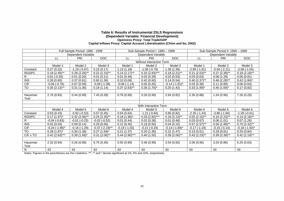
Table 6 reports the 2SLS when the capital account liberalization is employed as a

proxy for capital inflows. Again, the Hausman test results indicate that there is no different

between the estimates from OLS and 2SLS instrumental variable. The results are similar to

that obtained with the OLS regression, with the only notable difference being that the

interaction terms is statistically significant in all except two specifications. The exceptions are

Model 2 in the full sample and the first sub-sample; note however, that in the full sample it is 6 These results, however, are not reported but available upon request.

13

significant at the 10% level, probably reflecting the strength of the relationship in the 1990s.

Thus, if anything, the 2SLS results provide somewhat greater support to the Rajan-Zingales

hypothesis.

Pooled Mean Group Estimations Results

Table 7 reports estimates of Models (2) and (3) that utilize the pooled mean group

estimator, which imposes common long-run effects. This table presents estimates of the long-

run coefficients, the adjustment coefficients and Hausman test statistics. The lag order is first

chosen in each country on the unrestricted model by the Akaike information criterion (AIC),

subject to a maximum lag of 1. Then, using these AIC-determined lag orders, homogeneity is

imposed. The results indicate that the joint Hausman test statistic fails to reject the null

hypothesis and this reveals that the data do not reject the restriction of common long-run

coefficients. Besides, the Hausman test also indicates that the pooling restrictions cannot be

rejected for five independent variables. The coefficients of real GDP per capita and

institutions are positive and statistically significant throughout. The private capital inflows

variable also enters significantly in Models 2 and 3. On the other hand, in Models 4 –6 when

the interaction term is included in the model, the capital inflows variable loses significance at

conventional levels. Note, however, that the interaction term enters with a large and highly

significant positive coefficient in Models 4 – 6. These results, therefore, provide strong

support for the Rajan-Zingales hypothesis. The joint Hausman test of these models also

indicates that the data do not reject the restriction of common long-run coefficients, but the

poolability of real interest rate coefficient is rejected.

Table 8 repeats the pooled mean group estimator analysis with three capital market

development indicators, namely stock market capitalization, total share value traded and

number of companies listed. These indicators are only available for 22 developing countries7

and the sample period spans the period 1980 – 2000, except for the number of companies

listed, for which data is only available for the period 1988 – 2000. Both the real GDP per

capita and real interest rate retain their positive sign, but only real GDP per capita is

statistically significant in all models. The institutional quality variable is statistically significant

in determining market capitalization and total share value traded, but is significant only at the

10% in the regression that explains total number of companies listed. The capital inflows

variable is a statistically significant determinant of stock market capitalization and total share

value traded. In contrast, trade openness has a significant influence on market capitalization

and number of companies listed. In Models 4 – 6, the interaction term is statistically significant

at the 1% level in two out of three models and significant at the 10% level in the third.

7 The cross-country analysis is not conducted for these capital market development indicators - stock market capitalisation, total share value traded and number of companies listed due to small sample size (N = 22).

14

Interestingly, trade openness and capital inflows each have an independent statistically

significant influence in two out of three specifications. These findings suggest that the Rajan-

Zingales hypothesis applies not only to the development of the banking system, but also to

the development of the capital market.

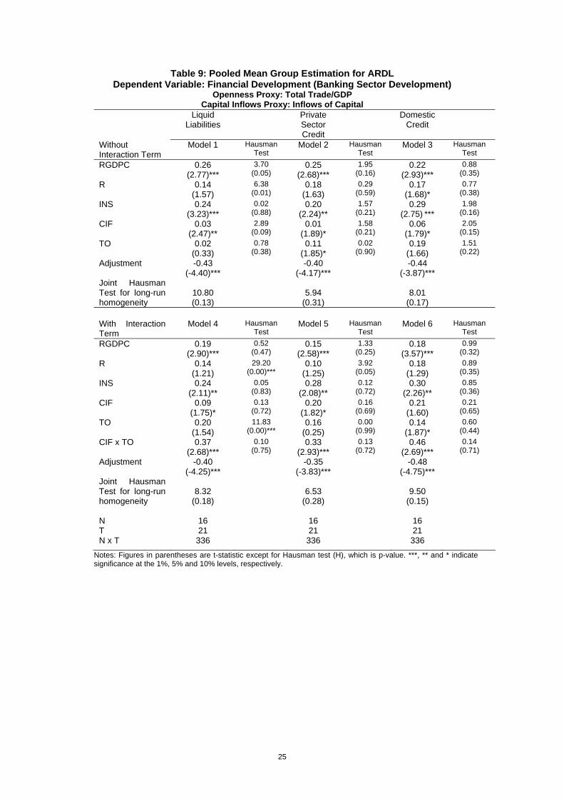
Table 9 repeats the analysis carried out in Table 7, using a different capital inflows

proxy, namely inflows of capital that consists of foreign direct investment and portfolio

investment8. This variable is only available for 16 developing countries. The lag order of AIC

is restricted to a maximum lag of 1 and the Hausman test statistic fails to reject the null

hypothesis of common long-run coefficients. Real GDP per capita and institutions retain their

positive sign and are both statistically significant. The inflows of capital is significant at the

10% level in Models 2 and 3. The estimated coefficients of the interaction term in Model 4 – 6

are both large and highly significant. These findings suggest that the results obtained in Table

7 are robust to changes in the measurement of capital account openness.

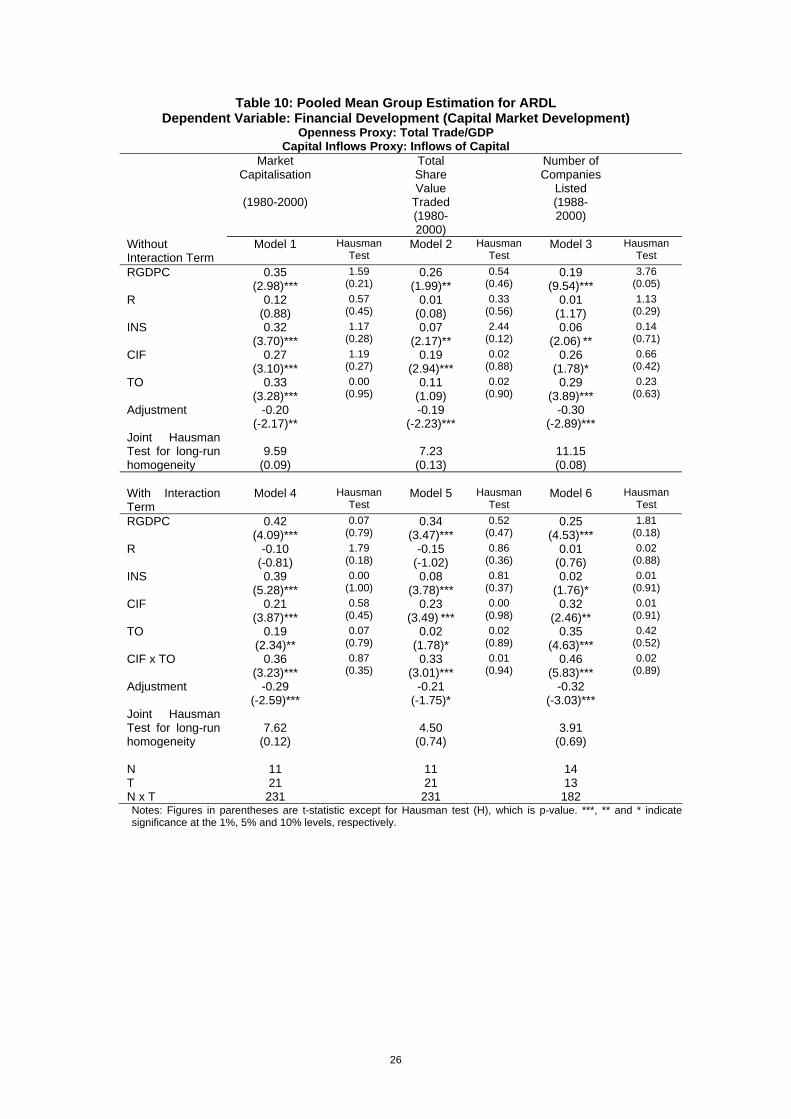
Table 10 repeats the analysis of Table 8 with the alternative proxy for capital inflows.

Again, real GDP per capita remains statistically significant in all specifications, while

institutional quality is now significant in all but one models (the exception being Model 6

where it is significant at the 10% level). Interestingly, the new capital inflows proxy, which

consists of foreign direct investment and portfolio investment, is positive and highly significant

in all specifications. In addition, the interaction term is highly significant in all three models.

These findings suggest that support for the Rajan-Zingales hypothesis is, if anything, even

stronger when the alternative proxy for capital account openness is utilised.

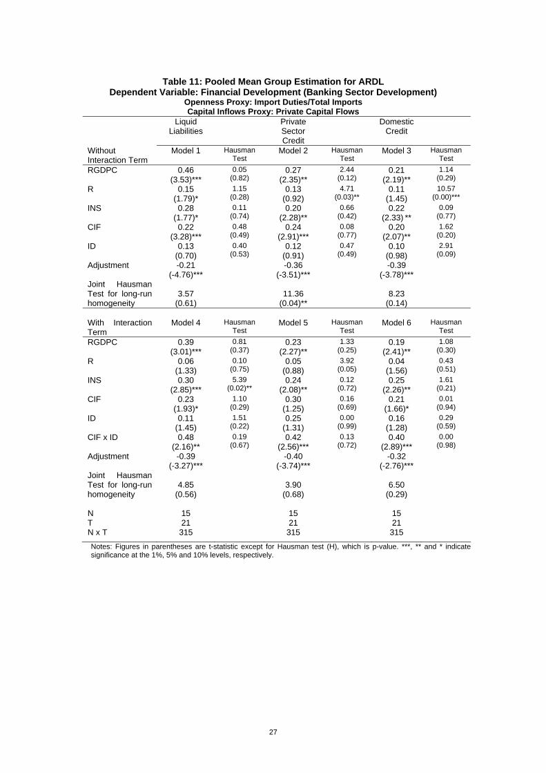
The estimated pooled mean group results when import duties indicator9 is employed

as an alternative proxy for trade openness are reported in Table 11. This indicator is found to

be statistically insignificant while real GDP per capita, institutions and capital inflows are

statistically significant in all models. However, models containing the interaction term

demonstrate that the interaction between capital inflows and import duties has a positive and

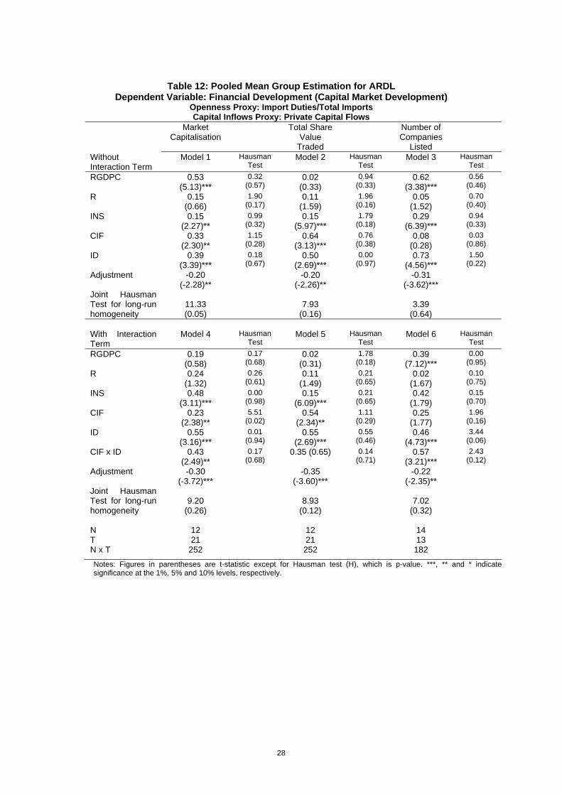
highly significant influence on financial development. Table 12 reports the analysis of Table

11 with the alternative proxy for financial development, namely capital market development

indicators. The import duties and institutions are statistically significant for three models,

whereas real GDP per capita and capital inflows are significant in two out of three models.

Again, the estimated coefficients of the interaction term are both large and significant in

Models 4 and 6. Thus, the main finding of our paper, namely that the trade openness has an

independent influence on financial development is robust to changes in the measurement of

both capital and trade account openness.

8 The capital account liberalization proxy constructed by Chinn and Ito (2002) is not employed in the panel data analysis even though the data is available from 1977 - 1999. This indicator is computed using the principal component analysis and most of the countries have no variation of capital account liberalization measurement throughout the year except in the mid 1990s. 9 The import duties/total imports (ID) indicator was first converted using this formula: (1 – ID/100).

15

5.0 Conclusions

The evidence presented utilising cross-country regressions and panel data analysis in

a group of developing countries, provides varying degrees of support to the Rajan and

Zingales (2003) hypothesis – that simultaneous opening of both the capital and trade

accounts will promote financial development. The evidence is at its strongest when we utilise

dynamic panel estimation techniques, and is robust to alternative measures of both trade

account and capital account openness. The evidence remains valid for a variety of financial

development indicators, including 3 indicators of banking system development and 3

indicators of capital market development.

Our findings also suggest that among the conventional determinants of financial

development real GDP per capita is the most robust one, while as suspected by several

authors in the past, the influence of the real interest rate is, at best, very weak and statistically

insignificant. We also find that institutional quality is a robust and statistically significant

determinant of financial development, providing support to the case made by Arestis and

Demetriades (1997, 1999). There is also some evidence to suggest that capital inflows have

an independent positive influence on financial development, independently of their influence

through the interaction term, especially so in the case of capital market development. Finally,

trade openness is not found to have a separate independent influence on financial

development, irrespective of which measure is employed. In terms of policy implications, our

findings suggest that simultaneously stimulating foreign capital inflows and trade openness,

improving institutions and economic development will encourage financial development.

References:

16

Acemoglu, D., Johnson, S. and Robinson, J.A. (2001) The Colonial Origins of Comparative Development: An Empirical Investigation. American Economic Review, 91, 1369 – 1401.

Arestis, P. and P. Demetriades. (1997) Financial Development and Economic Growth:

Assessing the Evidence. Economic Journal, 107, 783—799. Beck, T. (2003) Financial Development and International Trade. Is there a Link? The Work

Bank Group Working Paper, No. 2608. Beck, T., Demirgüç-Kunt, A. and Levine, R. (1999) A New Database on Financial

Development and Structure. The World Bank Group Working Paper. No.2784. Beck, T., Demirgüç-Kunt, A. and Levine, R. (2001) Law, Politics and Finance. The Work Bank

Group Working Paper, No. 2585. Beck, T., Demirgüç-Kunt, A. and Levine, R. (2003) Law, Endowment and Finance, Journal of

Financial Economics, 70, 137 – 181. Chinn, M. and Ito, H. (2002) Capital Account Liberalisation, Institutions and Financial

Development: Cross Country Evidence. NBER Working Paper 8967. Demetriades, P.O. and Hussein, K. (1996) Does Financial Development Cause Economic

Growth? Time Series Evidence from 16 Countries. Journal of Development Economics, 51, 387-411.

Demetriades, P.O. and Luintel, K.B. (1997) The Direct Costs of Financial Repression:

Evidence from India. The Review of Economics and Statistics, 79, 311 – 320. Demetriades, P. and Andrianova, S. (2004) ‘Finance and Growth: What We Know and What

We Need to Know’ in C. Goodhart, (ed), Money, Finance and Growth, Routledge, forthcoming

Demirgüç-Kunt, A. and Maksimovic, V. (1998) Law, Finance and Firm Growth, Journal of

Finance, 53, 2107 – 2137. Fry, M.J. (1997) In Defence of Financial Liberalisation. Economic Journal, 107 442 , 754–770. Goodhart, C. (2004) Money, Finance and Growth, Routledge, forthcoming (2004) Hausman, J. (1978) Specification Tests in Econometrics, Econometrica, 46, 1251 – 1271. King, R.G. and Levine, R. (1993a) Finance and Growth: Schumpeter Might be Right.

Quarterly Journal of Economics, 108, 717-737. King, R.G., Levine, R., (1993b). Finance, entrepreneurship and growth. Journal of Monetary

Economics, 32, 1–30. Klein, M and Olivei, G. (1999) ‘Capital Account Liberalisation, Financial Depth and Economic

Growth’. Federal Reserve Bank of Boston Working Paper, 99-6. Knack, Stephen and Keefer, Philip (1995) Institutions and Economic Performance: Cross-

country Tests Using Alternative Institutional Measures, Economics and Politics, 207 – 227.

La Porta, R., Lopez-de-Silane, F., Shleifer, A and Vishny, R. W. (1997) Legal Determinants of

External Finance. Journal of Finance, 52, 1131 – 1150. Levine, R. (1997) Financial Development and Economic Growth: Views and Agenda. Journal

of Economic Literature, 35, 688-726.

17

Levine, R. (2001) International Financial Liberalisation and Economic Growth. Review of

International Economics, 9, 688 – 702. Levine, R. (2003) More on Finance and Growth: More Finance, More Growth? Federal

Reserve Bank of St. Louis Review, 85 (4), 31–46. Luintel, K.B. and Khan, M. (1999) A Quantitative Reassessment of the Finance-Growth

Nexus: Evidence from a Multivariate VAR. Journal of Development Economics, 60, 381-405.

McKinnon, R.I. (1973) Money and Capital in Economic Development. Brookings Institution,

Washington, DC. McKinnon, R.I. (1991) The Order of Economic Liberalization: Financial Control in the

Transition to a Market Economy. Johns Hopkins University Press. Pagano, M. and Volpin, P. (2001) The Political Economy of Finance. Oxford Review of

Economic Policy, 17, 502 – 519. Pesaran, M.H. and Smith, R.P. (1995) Estimating Long-run Relationship from Dynamic

Heterogeneous Panels. Journal of Econometrics, 68, 79 – 113. Pesaran, M.H., Shin, Y. and Smith, R.P. (1999) Pooled Mean Group Estimation of Dynamic

Heterogeneous Panels. Journal of American Statistical Association, 94, 621 – 634. Quinn, D.P. and Inclan, C. (1997) The Origins of Financial Openness: A Study of Current and

Capital Account Liberalisation. American Journal of Political Science, 41, 771 – 813. Rajan, R.G. and Zingales, L. (1998) Financial Dependence and Growth. American Economic

Review, 88, 559-586. Rajan, R. G. and Zingales, L. (2003) The Great Reversals: The Politics of Financial

Development in the Twentieth Century. Journal of Financial Economics, 69, 5 – 50. Saleryd, H. and Vlachos, J. (2002) Markets for Risk and Openness to Trade: How are they

Related. Journal of International Economics, 57, 369 – 395. Shaw, E.S. (1973) Financial Deepening in Economic Development. Oxford Univ. Press, New

York. World Bank (1997) Private Capital Flows to Developing Countries. The Road to Financial

Integration. Washington D.C: The World Bank and Oxford University Press.

Table 1: Descriptive Statistics N = 43 LL PRI DOC RGDPC R INS CIF TO

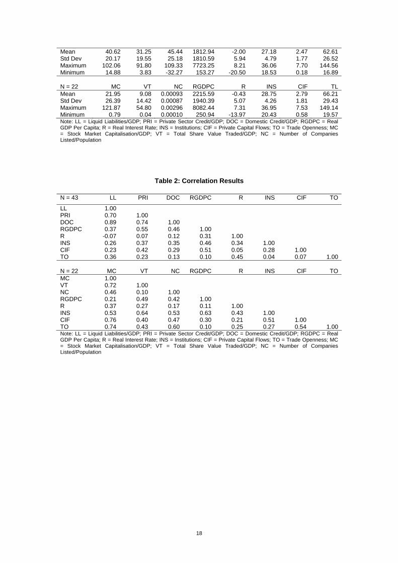
18

Mean 40.62 31.25 45.44 1812.94 -2.00 27.18 2.47 62.61 Std Dev 20.17 19.55 25.18 1810.59 5.94 4.79 1.77 26.52 Maximum 102.06 91.80 109.33 7723.25 8.21 36.06 7.70 144.56 Minimum 14.88 3.83 -32.27 153.27 -20.50 18.53 0.18 16.89 N = 22 MC VT NC RGDPC R INS CIF TL Mean 21.95 9.08 0.00093 2215.59 -0.43 28.75 2.79 66.21 Std Dev 26.39 14.42 0.00087 1940.39 5.07 4.26 1.81 29.43 Maximum 121.87 54.80 0.00296 8082.44 7.31 36.95 7.53 149.14 Minimum 0.79 0.04 0.00010 250.94 -13.97 20.43 0.58 19.57 Note: LL = Liquid Liabilities/GDP; PRI = Private Sector Credit/GDP; DOC = Domestic Credit/GDP; RGDPC = Real GDP Per Capita; R = Real Interest Rate; INS = Institutions; CIF = Private Capital Flows; TO = Trade Openness; MC = Stock Market Capitalisation/GDP; VT = Total Share Value Traded/GDP; NC = Number of Companies Listed/Population

Table 2: Correlation Results N = 43 LL PRI DOC RGDPC R INS CIF TO

LL 1.00 PRI 0.70 1.00 DOC 0.89 0.74 1.00 RGDPC 0.37 0.55 0.46 1.00 R -0.07 0.07 0.12 0.31 1.00 INS 0.26 0.37 0.35 0.46 0.34 1.00 CIF 0.23 0.42 0.29 0.51 0.05 0.28 1.00 TO 0.36 0.23 0.13 0.10 0.45 0.04 0.07 1.00 N = 22 MC VT NC RGDPC R INS CIF TO MC 1.00 VT 0.72 1.00 NC 0.46 0.10 1.00 RGDPC 0.21 0.49 0.42 1.00 R 0.37 0.27 0.17 0.11 1.00 INS 0.53 0.64 0.53 0.63 0.43 1.00 CIF 0.76 0.40 0.47 0.30 0.21 0.51 1.00 TO 0.74 0.43 0.60 0.10 0.25 0.27 0.54 1.00 Note: LL = Liquid Liabilities/GDP; PRI = Private Sector Credit/GDP; DOC = Domestic Credit/GDP; RGDPC = Real GDP Per Capita; R = Real Interest Rate; INS = Institutions; CIF = Private Capital Flows; TO = Trade Openness; MC = Stock Market Capitalisation/GDP; VT = Total Share Value Traded/GDP; NC = Number of Companies Listed/Population

19

Table 3: Results of OLS Regressions (Dependent Variable: Financial Development)

Openness Proxy: Total Trade/GDP Capital Inflows Proxy: Private Capital Flows

Full Sample Period: 1980 – 2000 Sub-Sample Period I: 1980 - 1989 Sub-Sample Period II: 1990 – 2000 Dependent Variable Dependent Variable Dependent Variable LL PRI DOC LL PRI DOC LL PRI DOC Without Interaction Term Model 1 Model 2 Model 3 Model 1 Model 2 Model 3 Model 1 Model 2 Model 3 Constant 0.88 (0.67) -0.04 (-0.02) 0.55 (0.39) 1.43 (1.26) -0.42 (-0.29) 1.59 (1.29) -2.31 (-1.45) -3.34 (-1.52) -1.72 (-0.84) RGDPC 0.16 (2.07)** 0.26 (2.37)** 0.17 (2.05)** 0.13 (2.22)** 0.23 (2.06)** 0.17 (1.89)* 0.20 (2.06)** 0.28 (2.29)** 0.19 (1.70)*

R 0.01 (0.17) 0.01 (0.18) 0.01 (0.19) 0.02 (0.62) 0.01 (0.20) 0.02 (0.69) 0.02 (0.52) 0.06 (0.98) 0.05 (1.03) INS 0.06 (0.15) 0.07 (0.14) 0.38 (0.85) 0.07 (0.25) 0.33 (0.91) 0.09 (0.32) 0.40 (2.04)** 0.35 (2.22)** 0.36 (2.13)** CIF -0.01 (-0.09) 0.11 (0.87) 0.03 (0.26) -0.01 (-0.13) 0.11 (0.79) 0.04 (0.39) 0.14 (2.05)** 0.22 (2.16)** 0.11 (1.90)* TO 0.32 (2.02)* 0.28 (1.37) 0.18 (1.06) 0.35 (2.02)* 0.24 (1.06) 0.18 (1.00) 0.36 (1.75)* 0.41 (1.86)* 0.22 (1.12) Adj R2 0.28 0.36 0.30 0.24 0.37 0.21 0.42 0.48 0.33 Normality 1.52 (0.46) 6.20 (0.06) * 2.41 (0.29) 2.95 (0.23) 0.73 (0.69) 0.04 (0.98) 1.90 (0.38) 4.26 (0.11) 5.15 (0.07)* B-P 0.45 (0.50) 0.06 (0.81) 0.03 (0.86) 0.27 (0.60) 0.38 (0.53) 0.19 (0.66) 0.12 (0.72) 0.04 (0.83) 0.16 (0.68) Ramsey 2.10 (0.12) 1.71 (0.18) 0.55 (0.65) 2.27 (0.10) 1.34 (0.27) 1.39 (0.26) 0.84 (0.48) 1.36 (0.27) 0.60 (0.61) With Interaction Term Model 4 Model 5 Model 6 Model 4 Model 5 Model 6 Model 4 Model 5 Model 6 Constant 2.53 (1.86) 0.97 (0.51) 1.64 (1.08) 2.14 (1.73) -1.56 (-0.99) 1.74 (1.29) -1.97 (-1.23) -3.18 (-1.41) -0.86 (-0.42) RGDPC 0.22 (2.73)** 0.29 (2.60)** 0.21 (2.37)** 0.16 (2.14)** 0.18 (2.26)** 0.17 (2.18)** 0.19 (2.09)** 0.21 (2.38)** 0.18 (1.79)*

R 0.02 (0.46) 0.03 (0.46) 0.03 (0.59) 0.03 (0.87) 0.01 (0.11) 0.02 (0.73) 0.03 (0.66) 0.06 (1.01) 0.07 (1.27) INS 0.08 (0.21) 0.02 (0.03) 0.29 (0.65) 0.16 (0.56) 0.48 (1.30) 0.07 (0.25) 0.46 (2.22)** 0.39 (2.27)** 0.37 (2.14)**

CIF -0.18 (-1.85)* -0.22 (-1.11) -0.43 (-1.67) -0.27 (-1.36) -0.25 (1.80)* -0.28 (-0.36) -0.24 (-1.25) -0.22 (-1.20) -0.20 (-1.91)*

TO 0.02 (0.14) 0.07 (0.25) 0.06 (0.29) 0.19 (0.91) 0.39 (1.86)* 0.14 (0.65) 0.14 (0.61) 0.32 (0.94) 0.19 (0.65) CIF x TO 0.50 (2.76)*** 0.31 (1.22) 0.34 (1.72)* 0.24 (1.76)* 0.50 (1.70)* 0.06 (0.30) 0.42 (2.26)** 0.40 (2.41)** 0.41 (2.18)**

Adj R2 0.42 0.38 0.36 0.29 0.43 0.22 0.46 0.51 0.40 Normality 1.86 (0.39) 5.21 (0.07)* 0.00 (0.99) 0.89 (0.64) 1.83 (0.40) 0.84 (0.65) 0.99 (0.61) 3.85 (0.15) 2.28 (0.32) B-P 0.01 (0.92) 0.19 (0.67) 0.00 (0.97) 0.11 (0.73) 2.45 (0.12) 0.11 (0.74) 0.05 (0.82) 0.00 (0.98) 0.10 (0.29) Ramsey 0.11 (0.95) 0.27 (0.84) 0.33 (0.80) 2.14 (0.12) 2.09 (0.12) 0.63 (0.60) 0.71 (0.55) 1.25 (0.31) 0.28 (0.84) N 43 43 43 43 43 43 43 43 43 Notes: Figures in the parentheses are the t-statistics except for the normality test, Breausch-Pagan heteroscedasticity test and Ramsey RESET tests, which are p-value. ***, ** and * denote significant at 1%, 5% and 10%, respectively.

20

Table 4: Results of OLS Regressions

(Dependent Variable: Financial Development) Openness Proxy: Total Trade/GDP

Capital Inflows Proxy: Capital Account Liberalisation (Chinn and Ito, 2002) Full Sample Period: 1980 – 1999 Sub-Sample Period I: 1980 - 1989 Sub-Sample Period II: 1990 – 1999 Dependent Variable Dependent Variable Dependent Variable LL PRI DOC LL PRI DOC LL PRI DOC Without Interaction Term Model 1 Model 2 Model 3 Model 1 Model 2 Model 3 Model 1 Model 2 Model 3 Constant 0.24 (0.19) -1.21 (-0.69) 0.14 (0.11) 0.97 (1.04) -0.97 (-0.74) 1.10 (1.12) -2.34 (-1.52) -4.45 (-2.02) -1.01 (-0.54) RGDPC 0.21 (2.67)** 0.32 (2.95)*** 0.22 (2.85)*** 0.17 (2.32)** 0.30 (3.05)*** 0.20 (2.74)*** 0.18 (2.04)** 0.31 (2.47)** 0.24 (2.04)**

R 0.02 (0.45) 0.01 (0.13) 0.01 (0.19) 0.01 (0.40) 0.02 (0.43) 0.01 (0.37) 0.02 (0.49) 0.07 (1.18) 0.03 (0.58) INS 0.11 (0.27) 0.28 (0.48) 0.35 (0.81) 0.04 (0.14) 0.22 (0.63) 0.12 (0.46) 0.31 (2.19)** 0.42 (2.27)** 0.57 (1.83)* CIF -0.09 (-1.13) 0.05 (0.47) -0.13 (-1.68) -0.09 (-1.24) 0.05 (0.49) -0.16 (1.79)* 0.11 (2.09)** 0.17 (2.15)** 0.14 (1.53) TO 0.36 (2.25)** 0.31 (1.40) 0.21 (1.33) 0.37 (2.24)** 0.35 (1.76)* 0.21 (1.45) 0.37 (2.26)** 0.44 (1.88)* 0.25 (1.25) Adj R2 0.32 0.37 0.33 0.28 0.36 0.29 0.53 0.50 0.35 Normality 1.50 (0.47) 5.29 (0.07) 1.83 (0.40) 3.21 (0.20) 2.30 (0.32) 0.52 (0.77) 1.78 (0.41) 2.68 (0.26) 0.18 (0.91) B-P 0.06 (0.80) 0.42 (0.52) 0.00 (0.95) 0.25 (0.62) 2.57 (0.11) 0.00 (0.96) 0.14 (0.71) 0.02 (0.89) 3.68 (0.05) Ramsey 1.96 (0.14) 1.62 (0.20) 0.93 (0.43) 2.41 (0.08) 1.49 (0.23) 1.96 (0.14) 0.77 (0.52) 1.98 (0.13) 0.62 (0.61) With Interaction Term Model 4 Model 5 Model 6 Model 4 Model 5 Model 6 Model 4 Model 5 Model 6 Constant 0.52 (0.43) -0.92 (-0.53) 0.54 (0.44) 0.50 (0.51) -1.11 (-0.78) 0.57 (0.57) -1.65 (-1.02) -4.25 (-1.79) -0.51 (-0.25) RGDPC 0.24 (3.19)*** 0.35 (3.24)*** 0.26 (3.50)*** 0.17 (2.47)** 0.31 (3.02)*** 0.21 (2.92)*** 0.22 (2.42)** 0.32 (2.37)** 0.24 (2.15)**

R 0.05 (1.06) 0.02 (0.30) 0.04 (0.90) 0.01 (0.36) 0.02 (0.42) 0.01 (0.34) 0.03 (-0.50) 0.06 (0.67) 0.01 (0.09) INS 0.16 (0.38) 0.01 (0.01) 0.02 (0.04) 0.13 (0.51) 0.20 (0.53) 0.02 (0.05) 0.26 (2.15)** 0.34 (2.31)** 0.41 (1.56)

CIF -0.28 (-2.23)** -0.23 (-1.39) -0.60 (-1.66) -0.24 (-1.54) -0.19 (-0.22) -0.08 (-1.78)* -0.16 (-1.27) -0.22 (-0.20) -0.23 (-0.89)

TO 0.32 (2.10)** 0.40 (1.74)* 0.30 (1.97)* 0.54 (2.93)*** 0.39 (1.49) 0.23 (1.54) 0.22 (1.27) 0.26 (0.64) 0.21 (1.00) CIF x TO 0.45 (2.80)*** 0.31 (1.46) 0.36 (2.45)** 0.21 (1.40) 0.51 (1.78)* 0.39 (2.12)** 0.35 (2.46)** 0.42 (2.28)** 0.32 (1.74)*

Adj R2 0.40 0.41 0.33 0.32 0.36 0.34 0.43 0.45 0.35 Normality 1.33 (0.51) 5.41 (0.07) 0.44 (0.80) 2.87 (0.23) 9.43 (0.01)** 2.29 (0.31) 1.54 (0.46) 2.63 (0.26) 0.09 (0.95) B-P 0.21 (0.64) 0.85 (0.35) 0.18 (0.67) 0.25 (0.62) 2.68 (0.10) 0.01 (0.91) 0.25 (0.62) 0.02 (0.88) 3.24 (0.07) Ramsey 0.09 (0.96) 0.33 (0.80) 1.16 (0.34) 5.10 (0.01)** 1.80 (0.17) 0.40 (0.75) 0.63 (0.59) 2.01 (0.13) 0.67 (0.57) N 43 43 43 43 43 43 43 43 43 Notes: Figures in the parentheses are the t-statistics except for the normality test, Breausch-Pagan (B-P) heteroscedasticity test and Ramsey RESET tests, which are p-value. ***, ** and * denote significant at 1%, 5% and 10%, respectively.

21

Table 5: Results of Instrumental 2SLS Regressions (Dependent Variable: Financial Development)

Openness Proxy: Total Trade/GDP Capital Inflows Proxy: Private Capital Inflows/GDP

Full Sample Period: 1980 – 2000 Sub-Sample Period I: 1980 - 1989 Sub-Sample Period II: 1990 – 2000 Dependent Variable Dependent Variable Dependent Variable LL PRI DOC LL PRI DOC LL PRI DOC Without Interaction Term Model 1 Model 2 Model 3 Model 1 Model 2 Model 3 Model 1 Model 2 Model 3 Constant 1.03 (0.77) 0.04 (0.02) 0.81 (0.56) 1.64 (1.40) -0.59 (-0.39) 2.03 (1.60) -2.76 (-1.68) -4.04 (-1.78)* -2.28 (-1.07) RGDPC 0.18 (1.81)* 0.21 (2.36)** 0.19 (1.99)** 0.11 (2.13)** 0.25 (2.04)** 0.11 (2.09)** 0.17 (2.16)** 0.19 (2.37)** 0.14 (2.03)**

R -0.01 (-0.02) 0.01 (0.25) 0.02 (0.42) 0.02 (0.66) 0.01 (0.18) 0.02 (0.76) 0.02 (0.53) 0.06 (0.98) 0.06 (1.01) INS 0.21 (0.47) 0.15 (0.28) 0.60 (1.29) 0.06 (0.19) 0.32 (0.87) 0.13 (0.42) 0.46 (2.42)** 0.51 (1.80)* 0.55 (2.06)**

CIF -0.04 (-0.37) 0.14 (1.03) 0.10 (0.94) -0.01 (-0.03) 0.09 (0.67) 0.01 (0.08) 0.13 (2.26)** 0.25 (2.15)** 0.04 (0.29) TO 0.31 (1.90)* 0.28 (1.33) 0.15 (0.88) 0.33 (1.91)* 0.25 (1.10) 0.15 (0.81) 0.34 (2.03)** 0.37 (1.61) 0.16 (0.74) Hausman Test

2.62 (0.85) 0.56 (0.99) 6.66 (0.35) 0.54 (0.99) 0.20 (0.99) 2.55 (0.86) 2.69 (0.84) 3.44 (0.75) 6.52 (0.36)

With Interaction Term Model 4 Model 5 Model 6 Model 4 Model 5 Model 6 Model 4 Model 5 Model 6 Constant 2.53 (1.84) 0.97 (0.51) 1.65 (1.06) 2.28 (1.81) -1.65 (-1.02) 2.09 (1.52) -2.35 (-1.43) -3.86 (-1.66) -1.28 (-0.61) RGDPC 0.16 (2.67)** 0.25 (2.19)** 0.20 (2.40)** 0.14 (2.09)** 0.17 (2.23)** 0.11 (2.10)** 0.15 (2.06)** 0.16 (2.23)** 0.14 (2.18)**

R 0.02 (0.53) 0.03 (0.49) 0.03 (0.70) 0.03 (0.89) 0.01 (0.12) 0.02 (0.76) 0.03 (0.67) 0.06 (1.01) 0.07 (1.26) INS 0.04 (0.06) 0.04 (0.08) 0.50 (1.10) 0.15 (0.49) 0.47 (1.26) 0.12 (0.38) 0.57 (2.57)** 0.56 (1.80)* 0.70 (2.32)**

CIF -0.17 (-2.48)** -0.13 (-1.01) -0.37 (-1.20) -0.21 (-1.25) -0.20 (-1.74)* -0.11 (-0.14) -0.17 (-1.19) -0.15 (-0.14) -0.18 (-1.92)*

TO 0.02 (0.07) 0.07 (0.27) 0.05 (0.26) 0.18 (0.88) 0.38 (1.87)* 0.13 (0.59) 0.13 (0.51) 0.28 (0.81) 0.25 (0.84) CIF x TO 0.47 (2.54)*** 0.29 (1.14) 0.27 (1.85)* 0.23 (1.28) 0.50 (2.01)* 0.26 (0.13) 0.43 (2.23)** 0.39 (2.38)** 0.42 (2.19)**

Hausman Test

1.43 (0.98) 2.35 (0.93) 5.72 (0.57) 0.38 (0.99) 5.72 (0.57) 2.49 (0.92) 2.06 (0.95) 3.24 (0.86) 5.25 (0.63)

N 43 43 43 43 43 43 43 43 43 Notes: Figures in the parentheses are the t-statistics. ***, ** and * denote significant at 1%, 5% and 10%, respectively.

22

Table 6: Results of Instrumental 2SLS Regressions (Dependent Variable: Financial Development)

Openness Proxy: Total Trade/GDP Capital Inflows Proxy: Capital Account Liberalisation (Chinn and Ito, 2002)

Full Sample Period: 1980 - 1999 Sub-Sample Period I: 1980 – 1989 Sub-Sample Period II: 1990 – 1999 Dependent Variable Dependent Variable Dependent Variable LL PRI DOC LL PRI DOC LL PRI DOC Without Interaction Term Model 1 Model 2 Model 3 Model 1 Model 2 Model 3 Model 1 Model 2 Model 3 Constant 0.27 (0.22) -1.19 (-0.67) 0.23 (0.17) 1.13 (1.18) -1.06 (-0.79) 1.39 (1.39) -2.89 (-1.81) -5.04 (-2.21) -2.08 (-1.05) RGDPC 0.18 (2.49)** 0.28 (2.26)** 0.22 (2.15)** 0.14 (2.17)** 0.32 (2.93)*** 0.18 (2.21)** 0.21 (2.03)** 0.27 (2.38)** 0.18 (2.18)**

R 0.01 (-0.26) 0.01 (0.20) 0.01 (0.11) 0.01 (0.49) 0.02 (0.39) 0.02 (0.53) 0.03 (0.63) 0.08 (1.28) 0.05 (0.81) INS 0.28 (0.65) 0.37 (0.61) 0.60 (1.36) 0.10 (0.08) 0.42 (0.60) 0.14 (0.54) 0.40 (2.37)** 0.46 (2.28)** 0.42 (1.84)*

CIF -0.06 (-0.76) 0.07 (0.59) -0.09 (-1.08) -0.08 (-1.14) 0.05 (0.45) -0.14 (-1.91)* 0.03 (0.38) 0.11 (0.89) 0.06 (0.64) TO 0.35 (2.13)** 0.31 (1.36) 0.19 (1.14) 0.37 (2.63)** 0.35 (1.76)* 0.20 (1.42) 0.33 (1.99)* 0.40 (1.69)* 0.17 (0.82) Hausman Test

2.76 (0.83) 0.44 (0.99) 7.43 (0.28) 0.76 (0.99) 0.26 (0.99) 2.94 (0.82) 2.35 (0.88) 1.34 (0.96) 7.26 (0.29)

With Interaction Term Model 4 Model 5 Model 6 Model 4 Model 5 Model 6 Model 4 Model 5 Model 6 Constant 0.53 (0.43) -0.92 (-0.53) 0.57 (0.45) 0.64 (0.64) -1.21 (-0.84) 0.85 (0.82) -2.35 (-1.43) -3.86 (-1.66) -1.28 (-0.61) RGDPC 0.17 (1.97)* 0.32 (2.56)** 0.25 (2.35)** 0.18 (1.96)* 0.33 (2.92)*** 0.16 (2.13)** 0.02 (2.15)** 0.16 (2.23)** 0.14 (2.18)**

R -0.04 (-0.83) -0.01 (-0.23) -0.02 (-0.52) 0.01 (0.44) 0.02 (0.38) 0.01 (0.48) 0.03 (0.67) 0.06 (1.01) 0.07 (1.26) INS 0.02 (0.03) 0.09 (0.14) 0.29 (0.66) 0.12 (0.45) 0.19 (0.50) 0.04 (0.15) 0.57 (2.57)** 0.56 (1.98)** 0.70 (2.32)**

CIF -0.24 (-1.96)* -0.16 (-1.29) -0.37 (-2.19)** -0.19 (-1.50) -0.21 (-0.24) -0.14 (-1.69)* -0.17 (-1.19) -0.15 (-0.14) -0.18 (-1.92)*

TO 0.28 (1.87)* 0.30 (1.38) 0.27 (1.69)* 0.21 (1.37) 0.20 (1.30) 0.22 (1.47) 0.13 (0.51) 0.28 (0.81) 0.25 (0.84) CIF x TO 0.42 (2.63)*** 0.39 (1.69)* 0.31 (2.06)** 0.44 (2.90)*** 0.40 (1.50) 0.39 (2.06)** 0.43 (2.23)** 0.39 (2.38)** 0.42 (2.19)**

Hausman Test

2.32 (0.94) 0.26 (0.99) 6.75 (0.45) 0.55 (0.99) 0.46 (0.99) 2.54 (0.92) 2.06 (0.95) 3.24 (0.86) 5.25 (0.63)

N 43 43 43 43 43 43 43 43 43 Notes: Figures in the parentheses are the t-statistics. ***, ** and * denote significant at 1%, 5% and 10%, respectively.

23

Table 7: Pooled Mean Group Estimation for ARDL Dependent Variable: Financial Development (Banking Sector Development)

Openness Proxy: Total Trade/GDP Capital Inflows Proxy: Private Capital Flows

Liquid Liabilities

Private Sector Credit

Domestic Credit

Without Interaction Term

Model 1 Hausman Test



RGDPC 0.16 (2.52)**

1.20 (0.27)

0.18 (2.27)**

0.87 (0.35)

0.19 (2.35)**

0.03 (0.85)

R 0.01 (1.62)

2.15 (0.14)

0.34 (1.49)

7.50 (0.01)

0.01 (1.26)

0.11 (0.74)

INS 0.18 (8.80)***

1.22 (0.27)

0.21 (2.31)**

0.28 (0.60)

0.25 (2.23) **

0.12 (0.73)

CIF 0.06 (0.38)

0.40 (0.53)

0.15 (2.81)***

0.85 (0.36)

0.24 (3.16)***

2.07 (0.15)

TO 0.04 (1.74)*

0.69 (0.41)

0.05 (0.53)

1.76 (0.18)

0.06 (1.08)

1.25 (0.26)

Adjustment -0.16 (-5.67)***

-0.16 (-5.32)***

-0.18 (-6.96)***

Joint Hausman Test for long-run homogeneity

2.79

(0.73)

8.50

(0.20)

2.85

(0.71)

With Interaction Term




RGDPC 0.23 (4.22)***

2.79 (0.09)

0.27 (4.76)***

0.97 (0.32)

0.20 (2.09)**

0.06 (0.81)

R 0.01 (0.81)

0.32 (0.57)

0.01 (0.74)

7.78 (0.01)**

0.03 (1.46)

0.07 (0.79)

INS 0.25 (2.23)**

1.17 (0.28)

0.30 (2.26)**

0.44 (0.51)

0.39 (2.16)**

0.65 (0.42)

CIF 0.15 (1.86)*

0.85 (0.36)

0.05 (1.55)

3.17 (0.07)

0.19 (1.16)

1.49 (0.22)

TO 0.31 (1.81)*

0.36 (0.55)

0.28 (0.95)

1.86 (0.17)

0.27 (1.32)

0.02 (0.88)

CIF x TO 0.46 (2.81)***

1.19 (0.27)

0.40 (3.02)***

3.00 (0.08)

0.43 (3.29)***

1.60 (0.21)

Adjustment -0.26 (-8.25)***

-0.20 (-8.04)***

-0.42 (-6.824)***


4.51

(0.61)

2.50

(0.76)

8.55

(0.20)

N 43 43 43 T 21 21 21 N x T 903 903 903

Notes: Figures in parentheses are t-statistic except for Hausman test (H), which is p-value. ***, ** and * indicate significance at the 1%, 5% and 10% levels, respectively.

24

Table 8: Pooled Mean Group Estimation for ARDL

Dependent Variable: Financial Development (Capital Market Development) Openness Proxy: Total Trade/GDP

Capital Inflows Proxy: Private Capital Flows Market

Capitalisation

Total Share Value

Traded

Number of Companies

Listed





RGDPC 0.31 (3.35)***

0.88 (0.35)

0.15 (2.54)**

2.03 (0.15)

0.59 (9.17)***

0.19 (0.66)

R 0.11 (1.74)*

7.89 (0.00)***

0.03 (0.49)

0.33 (0.57)

-0.01 (-0.31)

0.14 (0.70)

INS 0.14 (1.97)**

0.12 (0.73)

0.08 (3.99)***

0.42 (0.52)

0.08 (1.76)*

0.88 (0.35)

CIF 0.40 (2.11)**

0.43 (0.51)

0.33 (4.71)***

2.23 (0.13)

0.25 (1.07)

1.83 (0.18)

TO 0.27 (2.76)***

0.08 (0.77)

0.05 (1.34)

0.42 (0.52)

0.18 (3.32)***

3.62 (0.06)

Adjustment -0.16 (-5.67)***

-0.03 (-2.19)***

-0.29 (-4.32)***


9.66

(0.09)

6.98

(0.32)

10.42 (0.06)





RGDPC 0.26 (2.38)**

0.04 (0.84)

0.24 (2.17)**

0.07 (0.79)

0.32 (2.63)***

0.64 (0.42)

R 0.04 (0.47)

8.36 (0.00)***

0.10 (1.47)

0.00 (0.98)

-0.01 (-1.17)

0.99 (0.32)

INS 0.16 (2.18)**

0.56 (0.45)

0.12 (2.29)**

2.05 (0.15)

0.08 (0.59)

1.06 (0.30)

CIF 0.25 (2.32)**

0.59 (0.44)

0.28 (4.47) ***

1.37 (0.24)

0.32 (1.83)*

1.00 (0.32)

TO 0.17 (2.38)**

2.06 (0.15)

0.16 (1.71)*

2.05 (0.15)

0.28 (4.16)***

1.04 (0.31)

CIF x TO 0.41 (3.33)***

0.59 (0.44)

0.44 (3.04)***

1.47 (0.23)

0.49 (2.62)**

1.00 (0.32)

Adjustment -0.33 (-2.77)***

-0.25 (-2.66)***

-0.27 (-4.23)***


6.90

(0.44)

12.86 (0.05)

5.58

(0.47)

N 22 22 22 T 21 21 13 N x T 462 462 286


25

Table 9: Pooled Mean Group Estimation for ARDL Dependent Variable: Financial Development (Banking Sector Development)

Openness Proxy: Total Trade/GDP Capital Inflows Proxy: Inflows of Capital

Liquid Liabilities


Domestic Credit





RGDPC 0.26 (2.77)***

3.70 (0.05)

0.25 (2.68)***

1.95 (0.16)

0.22 (2.93)***

0.88 (0.35)

R 0.14 (1.57)

6.38 (0.01)

0.18 (1.63)

0.29 (0.59)

0.17 (1.68)*

0.77 (0.38)

INS 0.24 (3.23)***

0.02 (0.88)

0.20 (2.24)**

1.57 (0.21)

0.29 (2.75) ***

1.98 (0.16)

CIF 0.03 (2.47)**

2.89 (0.09)

0.01 (1.89)*

1.58 (0.21)

0.06 (1.79)*

2.05 (0.15)

TO 0.02 (0.33)

0.78 (0.38)

0.11 (1.85)*

0.02 (0.90)

0.19 (1.66)

1.51 (0.22)

Adjustment -0.43 (-4.40)***

-0.40 (-4.17)***

-0.44 (-3.87)***


10.80 (0.13)

5.94

(0.31)

8.01

(0.17)





RGDPC 0.19 (2.90)***

0.52 (0.47)

0.15 (2.58)***

1.33 (0.25)

0.18 (3.57)***

0.99 (0.32)

R 0.14 (1.21)

29.20 (0.00)***

0.10 (1.25)

3.92 (0.05)

0.18 (1.29)

0.89 (0.35)

INS 0.24 (2.11)**

0.05 (0.83)

0.28 (2.08)**

0.12 (0.72)

0.30 (2.26)**

0.85 (0.36)

CIF 0.09 (1.75)*

0.13 (0.72)

0.20 (1.82)*

0.16 (0.69)

0.21 (1.60)

0.21 (0.65)

TO 0.20 (1.54)

11.83 (0.00)***

0.16 (0.25)

0.00 (0.99)

0.14 (1.87)*

0.60 (0.44)

CIF x TO 0.37 (2.68)***

0.10 (0.75)

0.33 (2.93)***

0.13 (0.72)

0.46 (2.69)***

0.14 (0.71)

Adjustment -0.40 (-4.25)***

-0.35 (-3.83)***

-0.48 (-4.75)***


8.32

(0.18)

6.53

(0.28)

9.50

(0.15)

N 16 16 16 T 21 21 21 N x T 336 336 336


26

Table 10: Pooled Mean Group Estimation for ARDL Dependent Variable: Financial Development (Capital Market Development)

Openness Proxy: Total Trade/GDP Capital Inflows Proxy: Inflows of Capital

Market Capitalisation

(1980-2000)

Total Share Value

Traded (1980-2000)

Number of Companies

Listed (1988-2000)





RGDPC 0.35 (2.98)***

1.59 (0.21)

0.26 (1.99)**

0.54 (0.46)

0.19 (9.54)***

3.76 (0.05)

R 0.12 (0.88)

0.57 (0.45)

0.01 (0.08)

0.33 (0.56)

0.01 (1.17)

1.13 (0.29)

INS 0.32 (3.70)***

1.17 (0.28)

0.07 (2.17)**

2.44 (0.12)

0.06 (2.06) **

0.14 (0.71)

CIF 0.27 (3.10)***

1.19 (0.27)

0.19 (2.94)***

0.02 (0.88)

0.26 (1.78)*

0.66 (0.42)

TO 0.33 (3.28)***

0.00 (0.95)

0.11 (1.09)

0.02 (0.90)

0.29 (3.89)***

0.23 (0.63)

Adjustment -0.20 (-2.17)**

-0.19 (-2.23)***

-0.30 (-2.89)***


9.59

(0.09)

7.23

(0.13)

11.15 (0.08)





RGDPC 0.42 (4.09)***

0.07 (0.79)

0.34 (3.47)***

0.52 (0.47)

0.25 (4.53)***

1.81 (0.18)

R -0.10 (-0.81)

1.79 (0.18)

-0.15 (-1.02)

0.86 (0.36)

0.01 (0.76)

0.02 (0.88)

INS 0.39 (5.28)***

0.00 (1.00)

0.08 (3.78)***

0.81 (0.37)

0.02 (1.76)*

0.01 (0.91)

CIF 0.21 (3.87)***

0.58 (0.45)

0.23 (3.49) ***

0.00 (0.98)

0.32 (2.46)**

0.01 (0.91)

TO 0.19 (2.34)**

0.07 (0.79)

0.02 (1.78)*

0.02 (0.89)

0.35 (4.63)***

0.42 (0.52)

CIF x TO 0.36 (3.23)***

0.87 (0.35)

0.33 (3.01)***

0.01 (0.94)

0.46 (5.83)***

0.02 (0.89)

Adjustment -0.29 (-2.59)***

-0.21 (-1.75)*

-0.32 (-3.03)***


7.62

(0.12)

4.50

(0.74)

3.91

(0.69)

N 11 11 14 T 21 21 13 N x T 231 231 182 Notes: Figures in parentheses are t-statistic except for Hausman test (H), which is p-value. ***, ** and * indicate significance at the 1%, 5% and 10% levels, respectively.

27


Dependent Variable: Financial Development (Banking Sector Development) Openness Proxy: Import Duties/Total Imports Capital Inflows Proxy: Private Capital Flows

Liquid Liabilities


Domestic Credit





RGDPC 0.46 (3.53)***

0.05 (0.82)

0.27 (2.35)**

2.44 (0.12)

0.21 (2.19)**

1.14 (0.29)

R 0.15 (1.79)*

1.15 (0.28)

0.13 (0.92)

4.71 (0.03)**

0.11 (1.45)

10.57 (0.00)***

INS 0.28 (1.77)*

0.11 (0.74)

0.20 (2.28)**

0.66 (0.42)

0.22 (2.33) **

0.09 (0.77)

CIF 0.22 (3.28)***

0.48 (0.49)

0.24 (2.91)***

0.08 (0.77)

0.20 (2.07)**

1.62 (0.20)

ID 0.13 (0.70)

0.40 (0.53)

0.12 (0.91)

0.47 (0.49)

0.10 (0.98)

2.91 (0.09)

Adjustment -0.21 (-4.76)***

-0.36 (-3.51)***

-0.39 (-3.78)***


3.57

(0.61)

11.36

(0.04)**

8.23

(0.14)





RGDPC 0.39 (3.01)***

0.81 (0.37)

0.23 (2.27)**

1.33 (0.25)

0.19 (2.41)**

1.08 (0.30)

R 0.06 (1.33)

0.10 (0.75)

0.05 (0.88)

3.92 (0.05)

0.04 (1.56)

0.43 (0.51)

INS 0.30 (2.85)***

5.39 (0.02)**

0.24 (2.08)**

0.12 (0.72)

0.25 (2.26)**

1.61 (0.21)

CIF 0.23 (1.93)*

1.10 (0.29)

0.30 (1.25)

0.16 (0.69)

0.21 (1.66)*

0.01 (0.94)

ID 0.11 (1.45)

1.51 (0.22)

0.25 (1.31)

0.00 (0.99)

0.16 (1.28)

0.29 (0.59)

CIF x ID 0.48 (2.16)**

0.19 (0.67)

0.42 (2.56)***

0.13 (0.72)

0.40 (2.89)***

0.00 (0.98)

Adjustment -0.39 (-3.27)***

-0.40 (-3.74)***

-0.32 (-2.76)***


4.85

(0.56)

3.90

(0.68)

6.50

(0.29)

N 15 15 15 T 21 21 21 N x T 315 315 315


28


Dependent Variable: Financial Development (Capital Market Development) Openness Proxy: Import Duties/Total Imports Capital Inflows Proxy: Private Capital Flows

Market Capitalisation

Total Share Value

Traded

Number of Companies

Listed





RGDPC 0.53 (5.13)***

0.32 (0.57)

0.02 (0.33)

0.94 (0.33)

0.62 (3.38)***

0.56 (0.46)

R 0.15 (0.66)

1.90 (0.17)

0.11 (1.59)

1.96 (0.16)

0.05 (1.52)

0.70 (0.40)

INS 0.15 (2.27)**

0.99 (0.32)

0.15 (5.97)***

1.79 (0.18)

0.29 (6.39)***

0.94 (0.33)

CIF 0.33 (2.30)**

1.15 (0.28)

0.64 (3.13)***

0.76 (0.38)

0.08 (0.28)

0.03 (0.86)

ID 0.39 (3.39)***

0.18 (0.67)

0.50 (2.69)***

0.00 (0.97)

0.73 (4.56)***

1.50 (0.22)

Adjustment -0.20 (-2.28)**

-0.20 (-2.26)**

-0.31 (-3.62)***


11.33 (0.05)

7.93

(0.16)

3.39

(0.64)





RGDPC 0.19 (0.58)

0.17 (0.68)

0.02 (0.31)

1.78 (0.18)

0.39 (7.12)***

0.00 (0.95)

R 0.24 (1.32)

0.26 (0.61)

0.11 (1.49)

0.21 (0.65)

0.02 (1.67)

0.10 (0.75)

INS 0.48 (3.11)***

0.00 (0.98)

0.15 (6.09)***

0.21 (0.65)

0.42 (1.79)

0.15 (0.70)

CIF 0.23 (2.38)**

5.51 (0.02)

0.54 (2.34)**

1.11 (0.29)

0.25 (1.77)

1.96 (0.16)

ID 0.55 (3.16)***

0.01 (0.94)

0.55 (2.69)***

0.55 (0.46)

0.46 (4.73)***

3.44 (0.06)

CIF x ID 0.43 (2.49)**

0.17 (0.68)

0.35 (0.65) 0.14 (0.71)

0.57 (3.21)***

2.43 (0.12)

Adjustment -0.30 (-3.72)***

-0.35 (-3.60)***

-0.22 (-2.35)**


9.20

(0.26)

8.93

(0.12)

7.02

(0.32)

N 12 12 14 T 21 21 13 N x T 252 252 182


29

Appendix I Table AI: Definition and Source of the Data Variable Definition Source

Liquid Liabilities/GDP (%) (1980 – 2000, N = 43))

- Liquid liabilities the sum of currency and deposits in the central bank (M0), plus transferable deposits and electronic currency (M1), plus time and savings deposits, foreign currency transferable deposits, certificates of deposit, and securities repurchase agreements (M2), plus travelers checks, foreign currency time deposits, commercial paper, and shares of mutual funds or market funds held by residents.

World Development Indicator (World Bank CD-ROM, 2002)

Private Sector Credit/GDP (%) (1980 – 2000, N = 43))

- Financial resources provided to the private sector, such as through loans, purchases of non-equity securities, and trade credits and other accounts receivable, that establish a claim for repayment.

World Development Indicator

Domestic Credit Provided by Banking Sector (%) (1980 – 2000, N = 43))

- includes all credit to various sectors on a gross basis. The banking sector includes monetary authorities and deposit money banks, as well as other banking institutions where data are available (including institutions that do not accept transferable deposits but do incur such liabilities as time and savings deposits).


Stock Market Capitalisation/GDP (%) (1980 – 2000, N = 22))

Market capitalization (also known as market value) is the share price times the number of shares outstanding.

Beck et al. (1999).

Total Share Value Traded/GDP (%) (1980 – 2000, N = 22))

Stock traded refers to the total value of shares traded during the period. Beck et al. (1999).

Listed Domestic Companies/Population (%) (1988 – 2000, N = 22)

Listed domestic companies are the domestically incorporated companies listed on the country's stock exchanges at the end of the year.


Private capital flows, net total (US$) (1980 – 2000, N =43)

Net private capital flows consist of private debt and non-debt flows. Private debt flows include commercial bank lending, bonds, and other private credits; non-debt private flows are foreign direct investment and portfolio equity investment. Data are in current U.S. dollars.


Inflows of Capital (US$) (1980 – 2000, N = 16)

Capital inflows (sum of foreign direct investment and portfolio inflows) divided by GDP International Financial Statistics (IFS), lines 78bed + 78 bgd

Total Trade/GDP (%) (1980 – 2000, N = 43)

Trade is the sum of exports and imports of goods and services measured as a share of gross domestic product.


Import Duties/Total Imports (%) (1980 – 2000, N = 15)

Import duties comprise all levies collected on goods at the point of entry into the country. The levies may be imposed for revenue or protection purposes and may be determined on a specific or ad valorem basis, as long as they are restricted to imported products. Data are shown for central government only.


Deposit Interest Rate (%) (1980 – 2000, N = 43))

Deposit interest rate is the rate paid by commercial or similar banks for demand, time, or savings deposits.


30

Appendix II Table AII: The List of Developing Countries N = 43 (Banking sector Development) 1. Algeria 12. Gambia 23. Malta 34. Sri Lanka 2. Bangladesh 13. Ghana 24. Malaysia 35. Syrian Arab Republic 3. Bolivia 14. Guatemala 25. Mexico 36. Thailand 4. Botswana 15. Honduras 26. Morocco 37. Togo 5. Cameroon 16. India 27. Niger 38. Trinidad and Tobago 6. Chile 17. Indonesia 28. Nigeria 39. Tunisia 7. Costa Rica 18. Jamaica 29. Pakistan 40. Turkey 8. Cote d’lvoire 19. Jordan 30. Papua New Guinea 41. Uruguay 9. Ecuador 20. Kenya 31. Philippines 42. Venezuela 10. Egypt 21. Korea 32. Senegal 43. Zimbabwe 11. El Salvador 22. Malawi 33. Sierra Leone Note: Argentina and Brazil are not included in the sample due to these two countries have very high interest rate in 1990s and this may create an outlier and distort the model equilibrium.

N = 22 (Capital Market Development) 1. Chile 12. Morocco 2. Cote d'Ivoire 13. Nigeria 3. Egypt 14. Pakistan 4. India 15. Philippines 5. Indonesia 16. Sri Lanka 6. Jamaica 17. Thailand 7. Jordan 18. Trinidad and Tobago 8. Kenya 19. Turkey 9. Korea 20. Uruguay 10. Malaysia 21. Morocco 11. Mexico 22. Nigeria

capital inflows, trade openness and financial development ...fm · saving mobilisation and...

Documents