capital flows to emerging market economies · capital flows to emerging market economies shaghil...

Capital Flows to Emerging Market Economies

Shaghil Ahmed and Andrei Zlate Federal Reserve Board*

XVI Annual Inflation Targeting Seminar

of the Banco Central do Brasil Rio de Janeiro, Brasil, May 15-16, 2014

*The views in this presentation are the responsibility of the presenter and should not be interpreted as reflecting the views of the Board of Governors of the Federal Reserve System or any other person associated with the Federal Reserve System.

1

Motivation

Properties of Private EME Flows/Policy Responses

Previous Literature/Our Work

Empirical Specification

Results: Basic Model

Results: Extended Model

Results: Robustness

Conclusions

OUTLINE

2

Large EME capital flows and their volatility pose policy challenges

Policy tensions between EMEs and AEs

Questions: Main drivers?

Is post-crisis period different?

Have recent capital controls been effective?

Effects of unconventional U.S. monetary expansion?

MOTIVATION

3

Net private inflows have been volatile, although FDI has been relatively stable

PROPERTIES

4

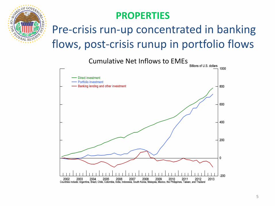
Pre-crisis run-up concentrated in banking flows, post-crisis runup in portfolio flows

PROPERTIES

Cumulative Net Inflows to EMEs

5

REER appreciations occurred post-crisis, but policymakers also appeared to intervene

Tempered policy rate increases

Several EMEs also used macroprudential measures and capital controls

REER Reserves Accumulation since 2005

POLICY RESPONSES

6

Surges

Ghosh et al (2012) o A variety of factors important

Forbes and Warnock (2012) o Global risk aversion matters a lot… o …but global interest rates/liquidity do not o Capital controls not effective

Common Component Byrne and Fiess (2011)

o U.S. interest rate crucial determinant

Exchange Rate Regime Ghosh et al (2012)

o Conditional on surge, magnitude of surge smaller the more flexible the exchange rate

Effects of U.S. LSAPs Fratzcher et al (2012)

o LSAP announcement and actual B/S changes significantly affect flows to EME-dedicated funds

Moore et al (2013) o Drop in U.S. yields raises share of foreign investments in EM bonds

PREVIOUS LITERATURE AND OUR WORK

7

Not identifying “surges” Common model with unusual changes in

explanatory variables and structural breaks

See also IMF (2011), Arias et al (2012)

Economic importance of different factors

Post-crisis period v. pre-crisis period

New data set of capital controls since 2009

U.S. LSAPs effects on BOP flows

Net vs. gross inflows

PREVIOUS LITERATURE AND OUR WORK

8

Panel, quarterly BOP data from 14 major emerging market economies over sub-periods from 2002:Q1 to 2013:Q2.

For NPI, alternatively use total net private inflows or portfolio net inflows; also report some regressions for gross private inflows

EMPIRICAL SPECIFICATION

9

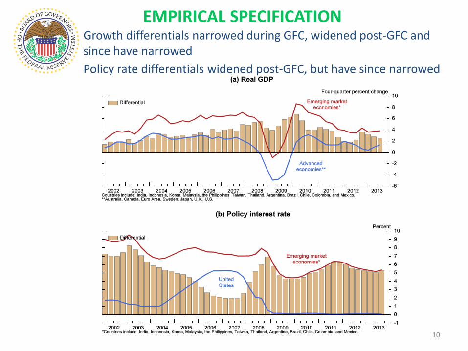
Growth differentials narrowed during GFC, widened post-GFC and since have narrowed Policy rate differentials widened post-GFC, but have since narrowed


10

Shifts in global risk sentiment have been accompanied by fluctuations in flows to EME funds


11

Several factors important in driving EME net capital inflows

Growth differentials, policy rate differentials, and global risk aversion all appear to matter for total net inflows

Global risk aversion and policy rate differentials important in explaining portfolio flows

RESULTS: BASIC MODEL

Table 2: Determinants of net private capital inflows: basic model

(1) (2) (3) (4)

(5) (6) (7) (8)

Dependent variable: Total net inflows/GDP

Portfolio net inflows/GDP

Interval: 2002q1 – 2008q2 2009q3 – 2013q2 2002q1 – 2008q2 2009q3 – 2013q2 Model: OLS FE OLS FE OLS FE OLS FE Growth diff. vs. AEs 0.38*** 0.36*** 0.25** 0.26** 0.13 0.079 -0.0041 0.022 (0.11) (0.12) (0.10) (0.10) (0.085) (0.086) (0.097) (0.092) Rate diff. vs. US 0.14*** -0.097 0.78*** 0.25 0.064** -0.062 0.38*** 0.34 (0.035) (0.069) (0.12) (0.25) (0.027) (0.051) (0.11) (0.23) VIX -0.083* -0.049 -0.17** -0.15** -0.13*** -0.11*** -0.11* -0.11* (0.049) (0.047) (0.071) (0.064) (0.038) (0.035) (0.067) (0.058) Trend 0.039 -0.012 -0.15* -0.13* -0.028 -0.051 -0.12 -0.11* (0.043) (0.043) (0.079) (0.071) (0.034) (0.032) (0.075) (0.064) Constant 0.0010 -1.98 8.89* 10.3** 2.22* 1.19 7.67* 6.29 (1.54) (1.74) (4.75) (4.68) (1.19) (1.29) (4.51) (4.22) Observations 364 364 224 224 364 364 224 224 R-squared 0.084 0.211 0.200 0.399 0.047 0.247 0.064 0.367

Note: Economies included are India, Indonesia, Malaysia, the Philippines, South Korea, Taiwan, and Thailand from emerging Asia, and Argentina, Brazil, Chile, Colombia, and Mexico from Latin America, as well as South Africa and Turkey. Standard errors are provided in parentheses, *** p<0.01, ** p<0.05, * p<0.1.

12

For total net inflows growth differentials, policy rate differentials, and global risk aversion all matter

Note: The fitted values and counterfactuals are based on the model with country fixed effects, estimated separately for the periods 2002:Q1-2008:Q2 and 2009:Q3 to 2013:Q2. The counterfactuals are the fitted values obtained under the assumption that a particular determinant was equal to its initial value for each interval.

Total Net Inflows

RESULTS: ECONOMIC IMPORTANCE

015

3045

USD

billio

n

2002q1 2003q1 2004q1 2005q1 2006q1 2007q1 2008q1

Fitted vs. counterfactual ex-growth

040

8012

0

2010q1 2011q1 2012q1 2013q1

Fitted vs. counterfactual ex-growth0

1530

45US

D bil

lion

2002q1 2003q1 2004q1 2005q1 2006q1 2007q1 2008q1

Fitted vs. counterfactual ex-policy rate

040

8012

0

2010q1 2011q1 2012q1 2013q1


015

3045

USD

billio

n

2002q1 2003q1 2004q1 2005q1 2006q1 2007q1 2008q1

Fitted vs. counterfactual ex-VIX

040

8012

02010q1 2011q1 2012q1 2013q1


Fitted value Counterfactual

13

Note: The fitted values and counterfactuals are based on the model with country fixed effects, estimated separately for the periods 2002:Q1-2008:Q2 and 2009:Q3 to 2013:Q2. The counterfactuals are the fitted values obtained under the assumption that a particular determinant was equal to its initial value for each interval.

Portfolio Net Inflows

RESULTS: ECONOMIC IMPORTANCE For portfolio net inflows, global risk aversion and policy rate differentials more important than growth differentials

-25

025

USD

billio

n

2002q1 2003q1 2004q1 2005q1 2006q1 2007q1 2008q1


-25

025

5075

2010q1 2011q1 2012q1 2013q1


-25

025

USD

billio

n

2002q1 2003q1 2004q1 2005q1 2006q1 2007q1 2008q1


-25

025

5075

2010q1 2011q1 2012q1 2013q1


-25

025

USD

billio

n

2002q1 2003q1 2004q1 2005q1 2006q1 2007q1 2008q1


-25

025

5075

2010q1 2011q1 2012q1 2013q1


Fitted value Counterfactual

14

Higher cumulative net inflows in the post-crisis period than the pre-crisis model would predict, with evidence of sea-change for portfolio inflows

Note: The model predictions are based on results from the model with fixed effects estimated over the period from 2002:Q1 to 2008:Q2, with the results reported in Table 2.

Shifting Behavior of Net Inflows since 2008-09

RESULTS: PRE-CRISIS V. POST-CRISIS

Net inflows significantly more sensitive to policy rate differentials in post-crisis period

Structural Break Tests for the Determinants of Net Inflows

RESULTS: STRUCTURAL BREAKS

(1) (2)

(3) (4)



Interval: 2002q1 – 2013q2 2002q1 – 2013q2 Model: OLS FE OLS FE Growth diff. vs. AEs 0.38*** 0.36*** 0.13 0.079 (0.10) (0.11) (0.085) (0.084) Rate diff. vs. US 0.14*** -0.097 0.064** -0.062 (0.033) (0.064) (0.027) (0.050) VIX -0.083* -0.049 -0.13*** -0.11*** (0.046) (0.044) (0.038) (0.034) Trend 0.039 -0.012 -0.028 -0.051 (0.041) (0.040) (0.034) (0.031)

D_post-crisis * Growth diff. vs. AEs -0.13 -0.10 -0.13 -0.057 (0.16) (0.16) (0.13) (0.13) D_post-crisis * Rate diff. vs. US 0.64*** 0.35 0.32*** 0.41* (0.14) (0.31) (0.11) (0.24) D_post-crisis * VIX -0.087 -0.10 0.015 -0.00042 (0.093) (0.088) (0.077) (0.069) D_post-crisis * Trend -0.19* -0.11 -0.093 -0.063 (0.099) (0.094) (0.082) (0.074) D_post-crisis 8.89 6.84 5.45 1.67 (5.62) (5.90) (4.65) (4.63) Constant 0.0010 -1.98 2.22* 1.19 (1.44) (1.61) (1.20) (1.26) Observations 588 588 588 588 R-squared 0.132 0.280 0.074 0.309

Note: The estimation excludes the crisis period from 2008:Q3 to 2009:Q2. D_post-crisis is an indicator variable that equals 1 for the period 2009:Q3-2013:Q2. The fixed effects and the trend are allowed to vary across the pre-crisis and post-crisis periods. Economies included are the same as in Table 2. Standard errors are provided in parentheses, *** p<0.01, ** p<0.05, * p<0.1.

16

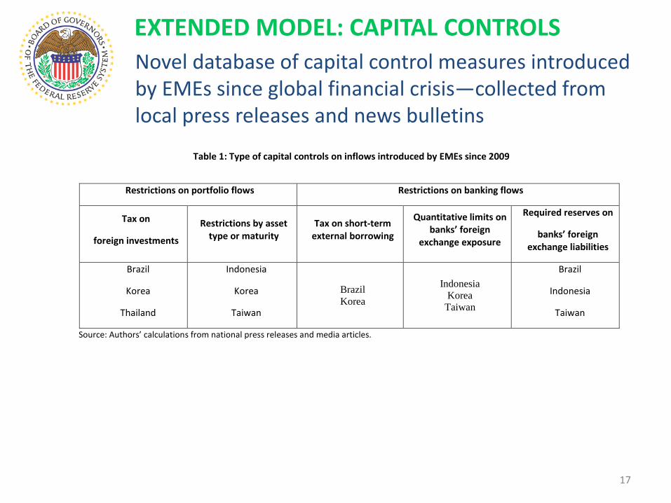
Novel database of capital control measures introduced by EMEs since global financial crisis—collected from local press releases and news bulletins

EXTENDED MODEL: CAPITAL CONTROLS

Table 1: Type of capital controls on inflows introduced by EMEs since 2009

Restrictions on portfolio flows Restrictions on banking flows

Tax on

foreign investments

Restrictions by asset type or maturity

Tax on short-term external borrowing

Quantitative limits on banks’ foreign

exchange exposure

Required reserves on

banks’ foreign exchange liabilities

Brazil

Korea

Thailand

Indonesia

Korea

Taiwan

Brazil Korea

Indonesia Korea

Taiwan

Brazil

Indonesia

Taiwan

Source: Authors’ calculations from national press releases and media articles.

17


Example, capital control measures in Brazil: 2009 Oct: IOF reinstated on foreign investment in equity and fixed

income. 2010 Oct: IOF on fixed income raised twice, extended to cover

foreign investment in mutual funds and derivatives. 2011 Jan: IOF on foreign investment in mutual funds lowered. 2011 Mar-Apr: IOF imposed on short-term external loans, then

extended to cover longer maturities. 2011 Apr: URR imposed on banks’ short FX positions. 2011 Dec: IOF removed for foreign investment in equities and certain

types of corporate bonds. 2012 Feb-Mar: IOF on short-term external loans extended again to

cover longer maturities. 2012 Jun-Dec: reduced maturity for external loans subject to IOF. 2012 Dec: increased deductible for URR on banks’ short FX positions. 2013 Jun: IOF on foreign investment in fixed income, derivatives

removed.

18

Database used to construct two variables on capital controls—number of measures in place and number of new measures introduced in any given quarter


19

LSAP indicator variables and U.S. 10-yr Treasury yield changes attributable to LSAPs used to estimate effect of U.S. unconventional monetary expansion

LSAP indicator variables LSAP purchases

Regress 10-yr U.S. Treasury yields on LSAPS one quarter ahead

Difference between yield and estimate of what it would be without LSAPs = component of yield attributable to LSAPs

EXTENDED MODEL: U.S. LSAPS

20

Net private EME inflows were dampened by capital control measures in recent years and amplified by LSAP announcements

EXTENDED MODEL: RESULTS

Net capital inflows to EMEs, the effects capital controls and LSAPs

(1) (2) (3) (4) (5) (6) Dependent variable: Total gross inflows/GDP Portfolio gross inflows/GDP Interval: 2009q3 – 2013q2 2009q3 – 2013q2 Model: FE FE FE FE FE FE Growth diff. vs. AEs 0.20* 0.23** 0.23** -0.014 0.0090 -0.0023 (0.11) (0.11) (0.11) (0.097) (0.095) (0.095) Rate diff. vs. US 0.27 0.29 0.22 0.33 0.34 0.25 (0.26) (0.26) (0.27) (0.23) (0.23) (0.24) VIX -0.12 -0.13* -0.16** -0.095 -0.079 -0.14* (0.075) (0.067) (0.078) (0.068) (0.060) (0.069) Cumulative controls (inflows) -0.61*** -0.60*** -0.59*** -0.55*** -0.55*** -0.57*** (0.20) (0.20) (0.21) (0.18) (0.18) (0.18)

U.S. Treasury yield 0.38 -0.029 (1.01) (0.91) LSAP announcements 0.82 1.02 (0.72) (0.64) LSAP effect on yields 0.43 0.97 (0.92) (0.81) Trend 0.039 -0.0085 -0.0090 -0.0099 0.011 -0.0091 (0.18) (0.081) (0.091) (0.16) (0.073) (0.080) Constant 4.10 6.97 8.74 4.20 2.44 6.27 (11.8) (4.92) (5.51) (10.7) (4.41) (4.83) Observations 208 208 195 208 208 195 R-squared 0.433 0.436 0.416 0.404 0.411 0.433 Note: D_LSAP announcements is an indicator variable equal to 1 for the quarters with the initial announcements of LSAPs and the decisions to continue them (see Figure 8, panel a). LSAP effect on yields is the difference between the actual 10-year U.S. Treasury bond yield and an estimate of what the yield would have been without LSAPs (see Figure 8, panel b and its footnote). Economies included are the same as in Table 2. Standard errors are provided in parentheses, *** p<0.01, ** p<0.05, * p<0.1.

21

Stronger evidence for effects of U.S. monetary policy on gross inflows, but effect of LSAP-related change in yields does not appear to be bigger

EXTENDED MODEL: RESULTS

Gross capital inflows to EMEs, the effects of capital controls and LSAPs

(1) (2) (3) (4) (5) (6) Dependent variable: Total gross inflows/GDP Portfolio gross inflows/GDP Interval: 2009q3 – 2013q2 2009q3 – 2013q2 Model: FE FE FE FE FE FE Growth diff. vs. AEs 0.32*** 0.28** 0.28*** 0.053 0.022 0.0046 (0.11) (0.11) (0.11) (0.068) (0.068) (0.068) Rate diff. vs. US -0.44 -0.41 -0.32 0.058 0.082 0.069 (0.28) (0.28) (0.29) (0.17) (0.17) (0.18) VIX -0.30*** -0.19*** -0.18** -0.23*** -0.14*** -0.14*** (0.082) (0.074) (0.081) (0.049) (0.045) (0.051) Cumulative controls (inflows) -0.015 -0.048 -0.14 -0.40*** -0.42*** -0.46*** (0.21) (0.21) (0.21) (0.13) (0.13) (0.13)

U.S. Treasury yield -2.63** -2.15*** (1.10) (0.67) LSAP announcements 1.35* 1.23** (0.79) (0.48) LSAP effect on yields -1.26 -0.68 (0.96) (0.61) Trend -0.56*** -0.11 0.0063 -0.43*** -0.062 -0.014 (0.20) (0.090) (0.095) (0.12) (0.055) (0.060) Constant 40.4*** 10.3* 4.60 30.4*** 5.67* 3.65 (12.9) (5.39) (5.72) (7.85) (3.27) (3.59) Observations 176 176 165 176 176 165 R-squared 0.410 0.400 0.435 0.337 0.322 0.322

Note: D_LSAP announcements is an indicator variable equal to 1 for the quarters with the initial announcements of LSAPs and the decisions to continue them (see Figure 8, panel a). LSAP effect on yields is the difference between the actual 10-year U.S. Treasury bond yield and an estimate of what the yield would have been without LSAPs (see Figure 8, panel b and its footnote). Economies included are the same as in Table 2. Standard errors are provided in parentheses, *** p<0.01, ** p<0.05, * p<0.1.

22

Results fairly robust to alternatives

Adding China and smaller economies in emerging Asia and Latin America Very similar results

Adding emerging European economies

VIX effects very similar Somewhat smaller effects of growth and interest rate

differentials

Using Credit Suisse’s GRAI instead of VIX Nearly identical results on growth and interest rate differentials Effects of risk appetite generally similar, although a bit less strong

Basic model using gross inflows instead of net

Effects of risk appetite bigger, but of growth and interest rate differentials smaller

ROBUSTNESS

23

Net capital flows to EMEs determined by several factors, including: growth differentials, policy rate differentials, global risk aversion Considering economic importance, all three variables

appear to be important for total net inflows For portfolio net inflows, global risk aversion and policy

rate differentials much more important than growth differentials

Pre-crisis model applied to post-crisis period underpredicts net inflows, esp. portfolio inflows Sensitivity of flows to policy rate differentials has

increased

CONCLUSIONS

24

Capital control measures introduced in recent years appear to have been effective

Significant effects of U.S. monetary expansion on EME net and gross inflows But U.S. unconventional policy is one among

several important determinants

No evidence that monetary expansion due to unconventional policy works in a different way

CONCLUSIONS

25

Gross inflows and gross outflows are positively correlated

EXTRA SLIDES

26

EXTRA SLIDES

Monetary policy response

27

LSAP events (Fratzcher, LoDuca and Straub, 2012)

QE1 initial announcements

QE2 initial announcements

EXTRA SLIDES

28

Effect of LSAPs on Treasury yields

Source: Asset purchases proxied by the change in end-of-quarter holdings of agency debt securities, mortgage-backed securities, and US Treasury securities, collected from FRB H.4.1 table.

-200

020

040

060

0U

SD

bill

ion

-20

24

6P

erce

ntag

e po

ints

2002q1 2004q1 2006q1 2008q1 2010q1 2012q1

US Treasury 10y yield LSAPsEffect of purchases

Effect of 1-quarter ahead LSAPs on yields Yields (ppt) = 3.87 –

0.002 * LSAPs[+1] (US$ bn)

On average, US$ 100 bn in LSAPs per quarter decreased yields by about 20 basis points, significant at the 10% level.

EXTRA SLIDES

29

Effect of capital controls on net inflows EXTRA SLIDES

Table 4: The effect of capital controls on net private capital inflows

(1) (2) (3) (4)

(5) (6) (7) (8)



Interval: 2009q3 – 2013q2 2009q3 – 2013q2 Model: OLS FE OLS FE OLS FE OLS FE Growth diff. vs. AEs 0.14 0.20* 0.23** 0.26** -0.087 -0.014 -0.015 0.024 (0.11) (0.11) (0.10) (0.11) (0.10) (0.097) (0.100) (0.095) Rate diff. vs. US 0.91*** 0.27 0.84*** 0.26 0.48*** 0.33 0.42*** 0.39 (0.11) (0.26) (0.12) (0.27) (0.11) (0.23) (0.11) (0.24) VIX -0.15* -0.12 -0.12 -0.14* -0.10 -0.095 -0.082 -0.10 (0.079) (0.075) (0.082) (0.075) (0.078) (0.068) (0.079) (0.068) U.S. Treasury yield 0.54 0.38 0.28 -0.31 0.13 -0.029 0.14 -0.13

(1.07) (1.01) (1.09) (1.01) (1.05) (0.91) (1.06) (0.91)

Cumulative controls -0.69*** -0.61*** -0.50*** -0.55*** (0.12) (0.20) (0.11) (0.18) New controls -0.22 0.21 0.28 0.40 (0.48) (0.45) (0.46) (0.41) L1.new controls -0.26 0.47 -0.54 -0.29 (0.48) (0.47) (0.47) (0.43) L2.new controls -0.97** -0.19 -0.79* -0.46 (0.49) (0.48) (0.47) (0.43) L3.new controls -1.21** -0.56 -0.45 -0.14 (0.51) (0.49) (0.49) (0.44) Trend 0.029 0.039 -0.098 -0.16 -0.017 -0.0099 -0.089 -0.13 (0.19) (0.18) (0.19) (0.18) (0.19) (0.16) (0.19) (0.16) Constant -0.54 4.10 4.70 9.72 2.95 4.20 5.21 8.25 (12.4) (11.8) (12.7) (11.7) (12.2) (10.7) (12.2) (10.5) Observations 208 208 224 224 208 208 224 224 R-squared 0.318 0.433 0.241 0.406 0.140 0.404 0.086 0.374

Note: Cumulative controls is the number of capital control measures introduced since 2009 that are in place in any given quarter. New controls is the number of new capital control measures introduced in any given quarter, with L1, L2, L3 indicating lagged values. Economies included are the same as in Table 2. Standard errors are provided in parentheses, *** p<0.01, ** p<0.05, * p<0.1. 30

Effect of capital controls on gross inflows EXTRA SLIDES

Table 5: The effect of capital controls on gross private capital inflows

(1) (2) (3) (4)

(5) (6) (7) (8)

Dependent variable: Total gross inflows/GDP

Portfolio gross inflows/GDP

Interval: 2009q3 – 2013q2 2009q3 – 2013q2 Model: OLS FE OLS FE OLS FE OLS FE Growth diff. vs. AEs 0.18 0.32*** 0.26** 0.32*** -0.00023 0.053 0.0014 0.070 (0.12) (0.11) (0.12) (0.11) (0.069) (0.068) (0.066) (0.068) Rate diff. vs. US 0.33** -0.44 0.24* -0.53* 0.16** 0.058 0.14* 0.10 (0.13) (0.28) (0.13) (0.28) (0.074) (0.17) (0.072) (0.18) VIX -0.31*** -0.30*** -0.29*** -0.34*** -0.24*** -0.23*** -0.21*** -0.22*** (0.092) (0.082) (0.093) (0.079) (0.053) (0.049) (0.054) (0.051) U.S. Treasury yield -2.28* -2.63** -2.39* -3.34*** -2.03*** -2.15*** -1.82** -2.03***

(1.24) (1.10) (1.24) (1.06) (0.72) (0.67) (0.71) (0.68)

Cumulative controls -0.57*** -0.015 -0.23*** -0.40*** (0.13) (0.21) (0.075) (0.13) New controls -0.47 0.17 0.44 0.43 (0.51) (0.44) (0.29) (0.28) L1.new controls -0.31 0.74 -0.15 -0.11 (0.51) (0.46) (0.29) (0.30) L2.new controls -0.52 0.51 -0.58* -0.47 (0.51) (0.47) (0.29) (0.30) L3.new controls -0.77 0.038 -0.47 -0.36 (0.54) (0.47) (0.31) (0.30) Trend -0.44** -0.56*** -0.56** -0.69*** -0.46*** -0.43*** -0.47*** -0.50*** (0.22) (0.20) (0.22) (0.19) (0.13) (0.12) (0.13) (0.12) Constant 37.2** 40.4*** 42.3*** 57.3*** 33.7*** 30.4*** 33.1*** 34.1*** (14.5) (12.9) (14.4) (12.6) (8.34) (7.85) (8.29) (8.10) Observations 176 176 192 192 176 176 192 192 R-squared 0.190 0.410 0.130 0.414 0.176 0.337 0.174 0.311

Note: Cumulative controls is the number of capital control measures introduced since 2009 that are in place in any given quarter. New controls is the number of new capital control measures introduced in any given quarter, with L1, L2, L3 indicating lagged values. Economies included are those in Table 2 minus India and Malaysia, for which gross inflows are only partially available. Standard errors are provided in parentheses, *** p<0.01, ** p<0.05, * p<0.1.

31

capital flows to emerging market economies · capital flows to emerging market economies shaghil...

Documents