capital flow components and the real exchange rate ... of content/pdf/vol14-2/05.pdf · capital...

International Journal of Business and Economics, 2015, Vol. 14, No. 2, 179-194

Capital Flow Components and the Real Exchange Rate:

Implications for India

Shashank Goel Indian Institute of Foreign Trade, India

V. Raveendra Saradhi

Indian Institute of Foreign Trade, India

Abstract

This paper analyzes the relationship between the net capital flow components and the

real exchange rate in India for the period 1996–1997 to 2012–2013. The empirical results

suggest that there is a strong case for further liberalization of foreign direct investment

flows, while greater caution is need in liberalization of portfolio and debt creating flows.

Key words: debt creating flows; foreign direct investment; foreign exchange reserves;

foreign portfolio flows; government consumption expenditure; real exchange rate

JEL classification: F30; F36; F40; F62; F65

1. Introduction

India has witnessed a large trend increase in cross border flows since the

introduction of the economic reforms process in the external sector in the early

1990s following the Balance of Payment (BoP) crisis. Net capital flows (NCF) to

India increased from 7.1 billion USD in 1990–1991 to 8.9 billion USD in 2000–

2001 and further to 89.3 billion USD during 2012–2013. Expressed as a percentage

of gross domestic product (GDP), the NCF increased from 2.2% of GDP in 1990–

1991 to 3.6% in 2010–2011 and further to 4.8% in 2012–2013. The increase in NCF

has been accompanied by a significant increase in its components comprising

Foreign Direct Investment (FDI) flows, portfolio flows, and debt creating flows in

the form of banking capital, external commercial borrowings of corporate entities,

and non-resident Indian deposits. The upswing in the capital mobility to India and

other emerging markets suffered a brief setback in the global financial crisis in 2008.

But after ebbing of the crisis, capital flows to India and other emerging market

economies rebounded in late 2009 and 2010.

Correspondence to: Indian Institute of Foreign Trade, IIFT Bhawan, B-21 Qutab Institutional Area, New

Delhi, 110016, India. Email: [email protected].

180 International Journal of Business and Economics

The main objective of this research is to comprehensively analyze the

relationship between the disaggregated NCF components: FDI flows, portfolio flows,

debt creating flows, and the real exchange rate (RER) along with other determinants

of RER. FDI, portfolio flows, debt creating flows and other capital flows,

government consumption expenditure, current account balance, and change in

foreign exchange reserves are used as explanatory variables, and the real effective

exchange rate (REER) index is the response variable. The estimation is conducted

on quarterly data on the Indian economy from 1996–1997 to 2012–2013. The

autoregressive distributed lag (ARDL) approach to cointegration is used to examine

the relationship between capital flow and other macroeconomic fundamentals and

the RER.

The most significant findings of the research are that among the components of

NCF, FDI flows are not found to be significantly associated with the RER

appreciation, but portfolio flows and debt creating flows are found to be associated

with RER appreciation in a statistically significant manner. Government

consumption expenditure is not found to be significantly associated with RER

appreciation, thereby limiting the role of fiscal policy in managing capital flows.

The rest of this paper is organized as follows. Section 2 attempts a review of

the literature on the impact of capital flows on the domestic economy. Section 3

describes the research methodology, and Section 4 presents the datasets used for

analysis. Section 5 reports the results of the econometric analysis, and Section 6

interprets the results and draws conclusions.

2. Theoretical Background and Literature Review

The concept of RER has been most widely used to analyze the impact of capital

flows on the economies of the developing countries. The impact of the capital

inflows on the domestic economy, which is mainly captured through the

appreciation of RER, is referred to as “the transfer problem.” The RER is an

important measure of the competitiveness of an economy as it is associated with

export growth. RER is the relative price of the domestic goods in terms of foreign

goods (e.g., US pizza per Indian pizza):

*RER e

P

P , (1)

where e is the nominal exchange rate, the relative price of domestic currency in

terms of foreign currency (e.g., dollar per rupee), P is the overall price level in the

domestic country, and *P is the overall price level in the foreign country.

The seminal works of Salter (1959), Swan (1960), Corden (1960), and

Dornbusch (1974) provide the theoretical framework to draw inferences on the

impact of capital flows on the RER in emerging market economies. In theory, a

surge in capital inflows in excess of domestic absorption capacity is associated with

an increase in expenditure and an appreciation of the RER. The effects of capital

Shashank Goel and V. Raveendra Saradhi 181

inflows on appreciation of RER can be derived from standard open economy models,

such as the intertemporal model of consumption and investment in an open economy

with capital mobility in the tradition of Irving Fischer (Calvo et al., 1996). The

theoretical models assume an economy with two goods—traded and nontraded—and

a representative consumer who maximizes utility by choosing the consumption of

the two goods over time (Mejia, 1999). In these models, a decline in world interest

rate induces income and substitution effects in the capital recipient country,

generating an increase in consumption and investment and a decline in savings

(which is the converse of higher consumption). Capital inflows generate higher

domestic demand of both tradeables and nontradeables in the economy. The rise in

demand for tradeables leads to a rise in imports and a widening of the trade deficit.

The tradeable goods are exogenously priced. The increase in demand of

nontradeables, however, leads to an increase in the relative price of nontradeables,

which are more limited in supply than the traded goods, so that the domestic

resources get diverted to their production. A higher relative price of the

nontradeables corresponds to RER appreciation. The extent of RER appreciation in

the economy will depend largely on the intertemporal elasticity of aggregate demand

and the income elasticity of demand and supply elasticity for nontradeable goods.

The intertemporal elasticity will determine the extent of consumption smoothing and

the distribution of expenditure increase through time. The elasticities for

nontradeables will determine the extent to which the surge in capital flows will

exercise pressure on the nontradeable prices. The appreciation of the RER is

indicative of the “Dutch disease effects” (Corden and Neary, 1982) that illustrates

the impact of natural resource booms or increases in capital flows on the

competiveness of the export-oriented sectors and the import-competing sectors.

The effect of net capital flows on the RER can be different depending upon the

composition of capital flows (Combes et al., 2011). In the financial account of BoP,

four distinctive types of capital flows usually appear, namely FDI, Portfolio

Investments, Debt Creating Flows, and Other Capital. The impact on RER depends

on the types of expenditure that each flow is tied to. In economies with supply

constraints, capital flows associated with the higher consumption put more pressure

on the relative prices of nontradeables, leading to an increase in their relative prices

and consequently to RER appreciation. On the other hand, capital flows associated

with higher investments, which have significant imported goods content, are less

likely to lead to RER appreciation. FDI flows could be related to investment in

imported machinery and equipment, which do not suffer from constraints in

domestic supply capacity and thus would have no effect on prices of domestic goods

and consequently almost no appreciation effect on RER. In addition, the spillover

effects of FDI may also improve local productive capacity through transfer of

technology and managerial know-how, thereby reducing pressure on the RER

(Javorick, 2004). FDI is also more stable as compared to portfolio investment and

other investment flows, such as bank lending. The effect of portfolio investment

flows on the RER might be different. If portfolio investment flows are oriented

towards the modernization of firms in recipient countries, which requires new


machinery and new product lines, the impact might be similar to that of FDI. But if

they are volatile investments for speculation that do not necessarily increase the

production capacity in the economy, then they would lead to a higher appreciation of

RER as compared to FDI (Lartey, 2007). The same applies to other investment

flows that can be either liabilities of the private or public sector of the economy.

Their impact would be different if they are used to finance purchase of

nontradeables, or tradeables or are used to finance exports production.

The behavior of RER in response to capital flow components has been

examined in several empirical studies. Among the early works, Elbadawi and Soto

(1994) studied the impact of the four disaggregated components—short-term capital

flows, long-term capital flows, portfolio investment, and FDI for the case of Chile

and found that long-term capital flows and FDI have a significant appreciating effect

on the equilibrium RER, while the short-term capital flows and portfolio

investments did not have any affect.

However, Athukorala and Rajapatirana (2003) found evidence that, for all

emerging market countries in their study, on average a 1% increase in other capital

flows brings a 0.56% appreciation in RER, but by contrast FDI inflows are

associated with depreciation rather than appreciation of the RER. The authors

attributed the depreciation effect of FDI on RER on the hypothesis that FDI

generally tends to have a more tradable bias compared to other types of capital flows.

Further, their analysis indicated that a given level of non-FDI capital flows led to a

far greater degree of appreciation of RER in Latin America, where the importance of

these flows in total capital inflows is also far greater as compared to emerging Asian

countries.

In another recent work, Bakardzhieva et al. (2010) reported that except FDI,

other forms of capital flows (i.e., debt, portfolio investments, aid) have a significant

positive impact on the RER. Their study reveals that FDI has no significant impact

on the RER. Based on these findings, they suggest that while FDI flows might lead

to RER appreciation in the short run when the economy receives the flows, its

impact is diluted over time as part of the flows start to leave the country in the form

of imports of machinery and other capital goods. In addition, the increase in

production induced by FDI can lead to downward pressure on prices and result in

RER depreciation.

In another important recent study, Combes et al. (2011) analyzed the impact of

capital inflows and their composition on the RER. Their results show that among

private flows, portfolio investment has the highest appreciation effect—almost seven

times that of FDI or bank loans. The authors suggest that the portfolio investment

flows, as compared to other private flows, are more volatile and speculative—

something generally associated with macroeconomic instability and no improvement

of productivity. They further argued that FDI is more stable than portfolio

investment and increases productive capacity through transfers of technology and

know-how. It is primarily for investment purposes and can lead to imports of new

machinery and equipment, which has limited impact on the RER. The appreciation

of the RER on account of loans from commercial banks is limited as in the case of


FDI. The authors suggest that bank loans can be directed to some extent to

investment financing like FDI, thereby improving productive capacity with a similar

inflation potential as that of FDI.

In a more recent study, Jongwanich and Kohpaiboon (2013) examined the

impact of capital flows on RERs in emerging Asian countries for the period 2000–

2009 using a dynamic panel-data model and found evidence that portfolio

investments brought in a faster speed of RER appreciation than FDI, though the

magnitude of appreciation by different types of capital flows were similar.

In the literature on the impact of capital flows on RERs in the Indian economy,

Biswas and Dasgupta (2012) examined the impact of capital inflows in India on the

RER using quarterly data for the period 1994–1995Q1 to 2009–2010Q4 using the

Johansen multivariate cointegration test. They found that FDI and workers’

remittances affected RER positively. The impulse response analysis results indicated

that shocks to FDI had a long-term positive impact on the RER, though it was

slightly negative in some of the ending periods. However, a very recent study by

Gaiha et al. (2014) explored the relationship between capital flows and RERs in

India for the period 2005–2012 using ordinary least squares estimation. They

reported that FDI flows had no significant impact on change in the RER. However,

portfolio flows and debt flows had a significant appreciation impact on the change in

the RER.

The cross-country studies on the effects of net capital flow components indicate

that different types of capital flows have different effects on the RER because they

act through different channels. In a recent study, Goel and Saradhi (2014) analyzed

the relationship between the aggregate NCF and other fundamentals for India for the

period 1996–1997 to 2012–2013 using the ARDL approach to cointegration. They

reported that net capital flows in India were positively associated with RER

appreciation, and the association was statistically significant. But no systematic

study is available on the relationship between the RER and different types of flows

(e.g., FDI or portfolio or debt flows) in India, especially for the more recent period.

This calls for further research on the subject.

3. Research Methodology

3.1 The Conceptual Model and the Selection of Model Variables

In this study, the following variables are used in order to investigate the

relationship between the disaggregated components of net capital flows and the RER

in the Indian economy.

REER

In order to measure the RER, the REER index is included in the baseline model.

The REER index is the weighted geometric average of the bilateral nominal

exchange rates of the home currency (Indian rupee, in this case) in terms of foreign

currencies adjusted by the ratio of domestic prices to the foreign prices (RBI, 2005):


1[( )( )] iwni i i

REER e e P P , (2)

where e is the exchange rate of Indian rupee against a numeraire (i.e., the

International Monetary Fund’s special drawing rights [SDRs]) in indexed form, i

e is

the exchange rate of foreign currency i against the numeraire (SDRs; i.e., SDRs per

currency i ) in indexed form, the i

w are the weights attached to foreign

currency/country i in the index, 1 1ni i

w , P is India’s wholesale price index, i

P

is the consumer price index of country i (i

CPI ), and n is the number of

countries/currencies in the index other than India.

FDI, PORT, DEBTCF, and OTHCAP

These are the main explanatory variables in the study. In order to measure the

volume of net capital flow components relative to the size of the economy, the ratio

of the disaggregated components of capital flows into the Indian economy in the

quarter and the quarterly GDP at market prices (at current prices) is used. FDI is the

ratio of the net FDI flows in the quarter and the quarterly GDP at market prices (at

current prices), PORT is the ratio of the net portfolio flows in the quarter and

quarterly GDP at market prices (at current prices), DEBTCF is the ratio of the

aggregate of net loans, banking capital, rupee debt service in the quarter and the

quarterly GDP at market prices (at current prices), and OTHCAP is the ratio of net

other capital in the quarter and quarterly GDP at market prices (at current prices).

GFCE

Government spending is an important fundamental determinant of RER, as it

adds to the aggregate demand and impacts the price levels in the economy. In order

to measure the size of public spending relative to the size of the economy,

government final consumption expenditure (GFCE) in the quarter as a proportion of

the quarterly GDP at market prices (at current prices) is used in the analysis. As a

sizeable portion of the government expenditure in India is devoted to imports of

essential commodities, the association of GFCE with REER is expected to be

ambiguous.

CAB

Current account balance has been included in the analysis as a sizeable portion

of capital flows in India is used to finance the current account deficit. Capital flows

to the extent of utilization for meeting the financing needs of the country are not

expected to cause adverse macroeconomic consequences. It is the surplus capital

flows over and above the financing requirements that have an adverse impact on the

economy. CAB is in the current account balance in the quarter as a proportion of the

quarterly GDP at market prices (at current prices). A more negative CAB is

expected to be associated with deprecation of the RER.

CFER


The Reserve Bank of India (RBI) maintains foreign exchange reserves in the

form of SDRs, gold, foreign currency assets, and reserve tranche position. CFER,

which is ratio of change in foreign exchange reserves in the quarter as a proportion

of the quarterly GDP at market prices (at current prices), is used as a proxy for

capturing the effect on RER of the change in rupee value of the components of

foreign exchange reserves, that is, SDRs, gold, foreign currency assets, and reserve

tranche position held by the RBI, which is different from the increase/decrease in

foreign reserves due to the overall balance of payments. An increase in foreign

exchange reserves, to the extent it is accompanied by prevention of an increase in

money supply (e.g., due to sterilization) is expected to lead to depreciation of the

RER for the Indian economy. On the other hand, an increase in foreign exchange

reserves accompanied by an increase in the money supply is expected to lead to

appreciation of the RER in the economy.

With this choice of variables, the functional relationship between the RER and

the explanatory variables is represented as follows:

{ , , , , , , }t t t t t t t t

REER f FDI PORT DEBTCF OTHCAP GFCE CAB CFER , (3)

where t refers to time.

To estimate the relationship between the response variable (REER) and the

components of the net capital flows (FDI, PORT, DEBTCF, and OTHCAP) and

other explanatory variables, the following log-linear specifications are used:

1 2 3

4 5 6 7,

t t t t

t t t t t

C FDI PORT DEBLNREER TCF

OTHCAP GFCE C B CFER ЄA

(4)

where tЄ is stochastic white noise at time t and LNREER is the natural log of

REER.

3.2 Empirical Methodology

3.2.1 Time Series Analysis of Variables

Before estimating the model, the response and explanatory variables are

separately subjected to unit roots tests using the augmented Dickey–Fuller (ADF)

test (Dickey and Fuller, 1979) and Philips-Perron (PP) test (Philips and Perron, 1988)

for testing the stationarity and order of integration. Usually, all variables are tested

with an intercept, with and without a linear trend.

3.2.2 Cointegration Analysis

In the econometric literature, different methodological approaches have been

used to empirically analyze the long-run relationships and dynamic interactions

between two or more time-series variables. The most widely used methods for

estimating the cointegrating vector between a set of time series variables include the

Engle and Granger (1987) two-step procedure and the maximum-likelihood


approach (Johansen and Juselius, 1990). Both these methods require that all the

variables under study are integrated of order one, I(1). This, in turn, requires that the

variables are subjected to pretesting to ascertain their orders of integration before

including them in particular cointegrating regressions. This introduces a certain

degree of uncertainty into the analysis. Apart from this, some of these test

procedures have very low power and do not have good small sample properties. One

of the relatively recent developments on univariate cointegration analysis is the

ARDL approach to cointegration introduced by Pesaran and Shin (1999) and further

extended by Pesaran et al. (2001). The main advantage of the ARDL method over

the Johansen and Juselius (1990) approach is that it allows for a mix of I(1) and I(0)

variables in the same cointegration equation. Another advantage is that the ARDL

test is more efficient, and the estimates derived from it are relatively more robust in

small sample sizes as compared to the traditional Johansen-Juselius cointegration

approach, which typically requires a large sample size for the results to be valid. In

addition, the choice of the ARDL bounds-testing procedure allows for both response

and explanatory variables to be introduced in the model with lags. This is a highly

plausible feature because, conceptually, a change in the economic variables may not

necessarily lead to an immediate change in another variable. In some cases, they

may respond to the economic developments with a lag, and there is usually no

reason to assume that all regressors should have the same lags. Because the ARDL

approach draws on the unrestricted error correction model, it is likely to have better

statistical properties than the traditional cointegration techniques. The ARDL

approach is particularly applicable in the presence of the disequilibrium nature of the

time series data stemming from the presence of possible structural breaks as happens

with most economic variables.

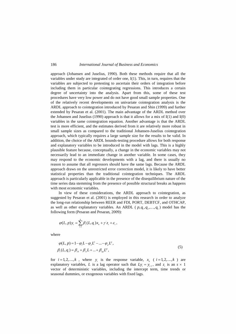
In view of these considerations, the ARDL approach to cointegration, as

suggested by Pesaran et al. (2001) is employed in this research in order to analyze

the long-run relationship between REER and FDI, PORT, DEBTCF, and OTHCAP,

as well as other explanatory variables. An ARDL (1 2

, , , ,k

p q q q ) model has the

following form (Pesaran and Pesaran, 2009):

'

1

( , ) ( , )k

t i i it t t

i

L p y L q x z

,

where

2

1 2

0 1

( , ) 1 ... ,

( , ) ... ,

p

p

qi

i i i i iqi

L p L L L

L q L L

(5)

for 1,2, ,i k , where t

y is the response variable, it

x ( 1,2, ,i k ) are

explanatory variables, L is a lag operator such that 1t t

Ly y

, and t

z is an s 1

vector of deterministic variables, including the intercept term, time trends or

seasonal dummies, or exogenous variables with fixed lags.


The ARDL procedure involves two stages. In the first stage, the existence of

the long-run relationship between the variables under investigation is tested by

computing the F statistics for testing significance of the lagged levels of the

variables in the error-correction form of the ARDL model. Once the existence of a

long-run relationship is established, in the second stage the long-run coefficients and

the error-correction model are estimated. Equation 5 is estimated by the ordinary

least squares method for all possible values of 0,1,2, ,p m (where m is the

maximum lag order) and 0,1,2, ,i

q m ( 1,2, ,i k ) for a total of 1( 1)km

different ARDL models. All models are estimated for the same sample period,

namely 1, 2, ,t m m n . Thereafter, one of the 1( 1)km

estimated models is

selected using one of the following four model selection criteria: the 2R criterion,

the Akaike information criterion (AIC), The Schwarz Bayesian criterion (SBC), or

the Hannan and Quinn criterion. Thereafter, the long-run coefficients and their

asymptotic standard errors for the selected ARDL model are computed.

4. Data Sources

The dataset comprises the quarterly data for the Indian economy for the period

1996–1997Q1 to 2012–2013Q4. The REER index used in the study is the monthly

trade-weighted 36 currency REER indices obtained from the Handbook of Statistics

published by the RBI (2014). The quarterly REER indices were obtained by

averaging the monthly indices for the quarter.

In this study, FDI, PORT, DEBTCF (which in turn comprises Loans, Net

Banking Capital, and Net Rupee Debt Service), OTHCAP, GFCE, and CAB, are

measured as ratios of their quarterly values to quarterly estimates of GDP at market

prices (at current prices; base year 2004–2005). The CFER is measured as a ratio of

the change in foreign exchange reserves (in rupees) from the end of the previous

quarter to the end of the present quarter to the quarterly estimates of GDP at market

prices (at current prices; base year 2004–2005). The data for net capital flow

components, current account balance, and foreign exchange reserves were obtained

from the Handbook of Statistics (RBI, 2014). The data for quarterly GDP at market

prices (at current prices) and GFCE base year 2004–2005 were obtained from the

National Account Statistics of the Central Statistical Office, Ministry of Statistics

and Programme Implementation.

5. Estimation Results

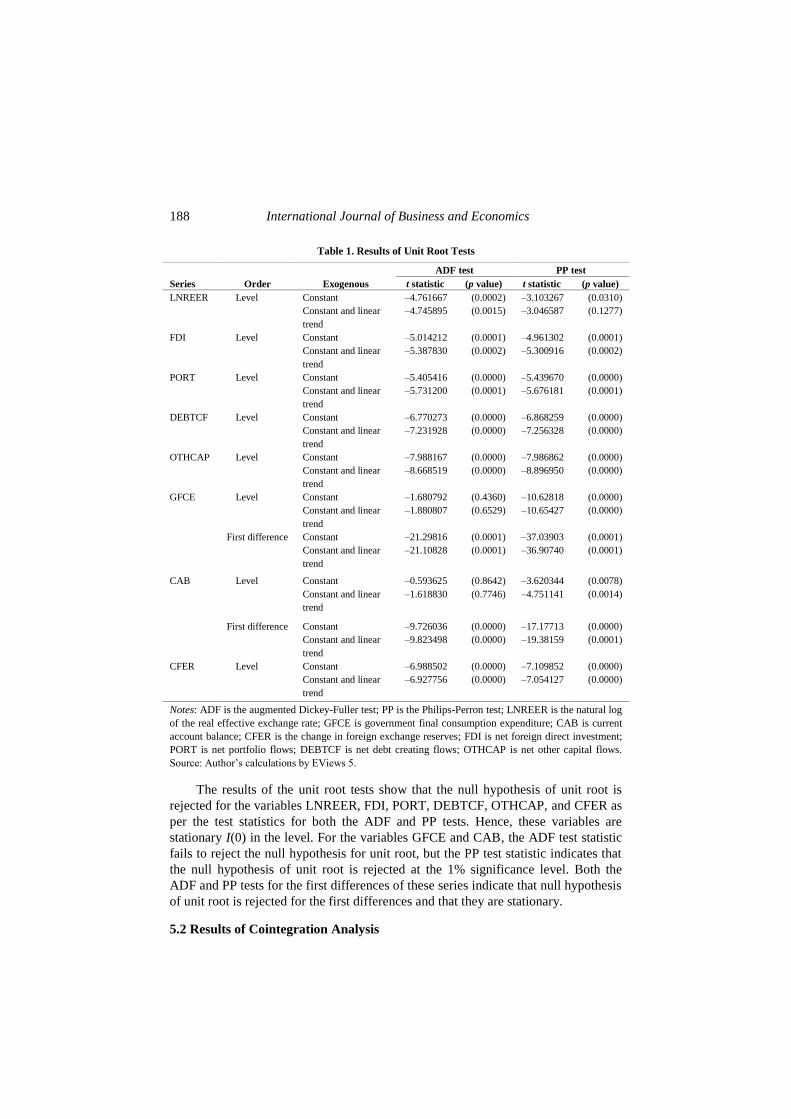
5.1 Stationary Properties of the Variables

For the quarterly data on variables for the period 1996–1997Q1 to 2012–

2013Q4, the results of the ADF test and PP test are presented in Table 1.


Table 1. Results of Unit Root Tests

Series Order Exogenous

ADF test PP test

t statistic (p value) t statistic (p value)

LNREER Level Constant –4.761667 (0.0002) –3.103267 (0.0310)

Constant and linear

trend

–4.745895 (0.0015) –3.046587 (0.1277)

FDI Level Constant –5.014212 (0.0001) –4.961302 (0.0001)

Constant and linear

trend

–5.387830 (0.0002) –5.300916

(0.0002)

PORT Level Constant

Constant and linear

trend

–5.405416

–5.731200

(0.0000)

(0.0001)

–5.439670

–5.676181

(0.0000)

(0.0001)

DEBTCF Level Constant

Constant and linear

trend

–6.770273

–7.231928

(0.0000)

(0.0000)

–6.868259

–7.256328

(0.0000)

(0.0000)

OTHCAP Level Constant

Constant and linear

trend

–7.988167

–8.668519

(0.0000)

(0.0000)

–7.986862

–8.896950

(0.0000)

(0.0000)

GFCE Level Constant –1.680792 (0.4360) –10.62818 (0.0000)

Constant and linear

trend

–1.880807 (0.6529) –10.65427 (0.0000)

First difference Constant –21.29816 (0.0001) –37.03903 (0.0001)

Constant and linear

trend

–21.10828 (0.0001) –36.90740 (0.0001)

CAB Level Constant –0.593625 (0.8642) –3.620344 (0.0078)

Constant and linear

trend

–1.618830 (0.7746) –4.751141 (0.0014)

First difference Constant –9.726036 (0.0000) –17.17713 (0.0000)

Constant and linear

trend

–9.823498 (0.0000) –19.38159 (0.0001)

CFER Level Constant –6.988502 (0.0000) –7.109852 (0.0000)

Constant and linear

trend

–6.927756 (0.0000) –7.054127 (0.0000)

Notes: ADF is the augmented Dickey-Fuller test; PP is the Philips-Perron test; LNREER is the natural log

of the real effective exchange rate; GFCE is government final consumption expenditure; CAB is current

account balance; CFER is the change in foreign exchange reserves; FDI is net foreign direct investment;

PORT is net portfolio flows; DEBTCF is net debt creating flows; OTHCAP is net other capital flows.

Source: Author’s calculations by EViews 5.

The results of the unit root tests show that the null hypothesis of unit root is

rejected for the variables LNREER, FDI, PORT, DEBTCF, OTHCAP, and CFER as

per the test statistics for both the ADF and PP tests. Hence, these variables are

stationary I(0) in the level. For the variables GFCE and CAB, the ADF test statistic

fails to reject the null hypothesis for unit root, but the PP test statistic indicates that

the null hypothesis of unit root is rejected at the 1% significance level. Both the

ADF and PP tests for the first differences of these series indicate that null hypothesis

of unit root is rejected for the first differences and that they are stationary.

5.2 Results of Cointegration Analysis


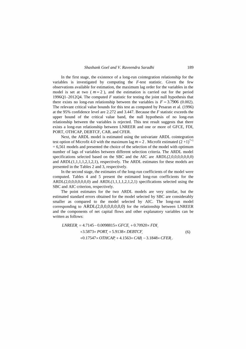
In the first stage, the existence of a long-run cointegration relationship for the

variables is investigated by computing the F-test statistic. Given the few

observations available for estimation, the maximum lag order for the variables in the

model is set at two ( 2m ), and the estimation is carried out for the period

1996Q1–2012Q4. The computed F statistic for testing the joint null hypothesis that

there exists no long-run relationship between the variables is 3.7906F (0.002).

The relevant critical value bounds for this test as computed by Pesaran et al. (1996)

at the 95% confidence level are 2.272 and 3.447. Because the F statistic exceeds the

upper bound of the critical value band, the null hypothesis of no long-run

relationship between the variables is rejected. This test result suggests that there

exists a long-run relationship between LNREER and one or more of GFCE, FDI,

PORT, OTHCAP, DEBTCF, CAB, and CFER.

Next, the ARDL model is estimated using the univariate ARDL cointegration

test option of Microfit 4.0 with the maximum lag 2m . Microfit estimated (2 +1)7+1

= 6,561 models and presented the choice of the selection of the model with optimum

number of lags of variables between different selection criteria. The ARDL model

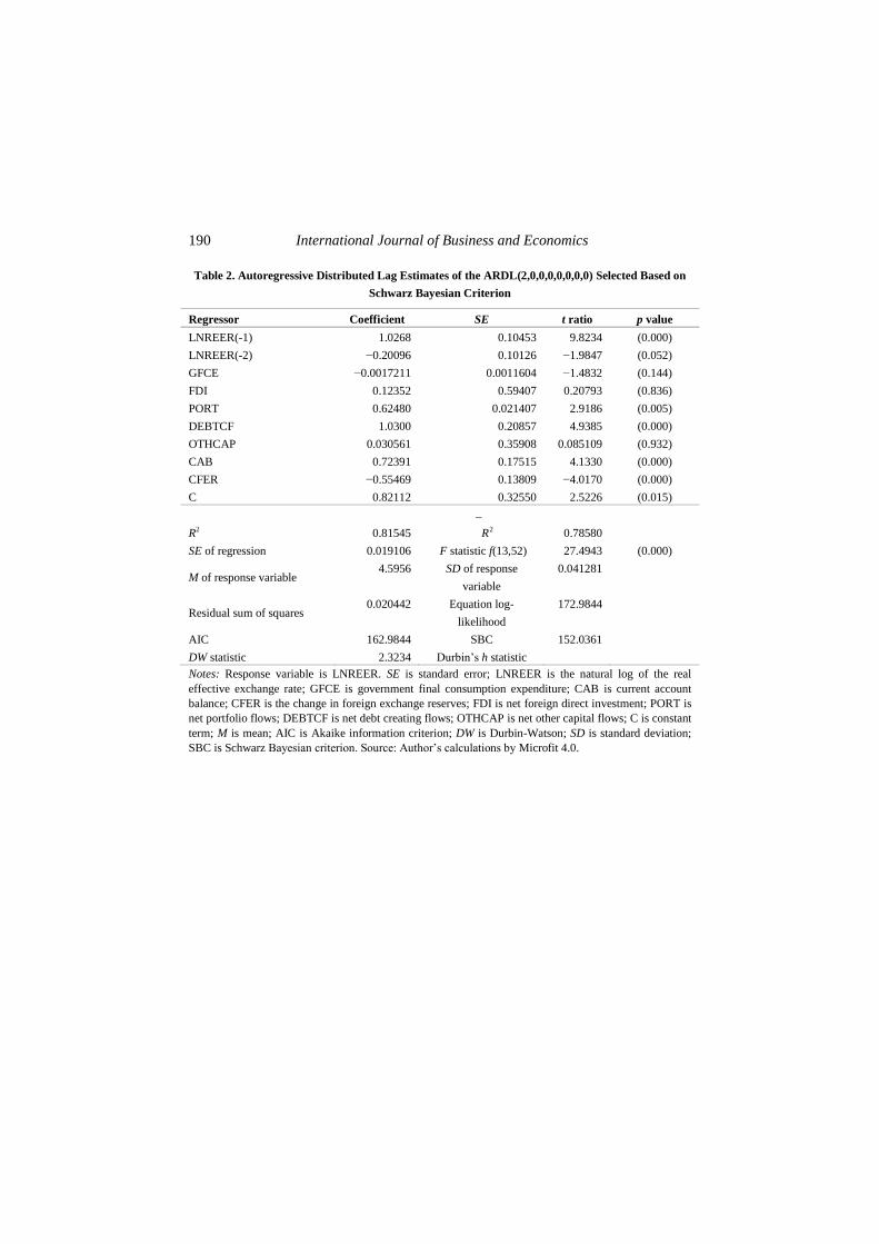
specifications selected based on the SBC and the AIC are ARDL(2,0,0,0,0,0,0,0)

and ARDL(1,1,1,1,2,1,2,1), respectively. The ARDL estimates for these models are

presented in the Tables 2 and 3, respectively.

In the second stage, the estimates of the long-run coefficients of the model were

computed. Tables 4 and 5 present the estimated long-run coefficients for the

ARDL(2,0,0,0,0,0,0,0) and ARDL(1,1,1,1,2,1,2,1) specifications selected using the

SBC and AIC criterion, respectively.

The point estimates for the two ARDL models are very similar, but the

estimated standard errors obtained for the model selected by SBC are considerably

smaller as compared to the model selected by AIC. The long-run model

corresponding to ARDL(2,0,0,0,0,0,0,0) for the relationship between LNREER

and the components of net capital flows and other explanatory variables can be

written as follows:

4.7145 0.0098815 0.70920

3.5873 5.9138

0.17547 4.1563 3.1848 .

t t t

t t

t t t

GFCE FDI

PORT DEBTCF

OTHCAP CAB CFER

LNREER

(6)


Table 2. Autoregressive Distributed Lag Estimates of the ARDL(2,0,0,0,0,0,0,0) Selected Based on

Schwarz Bayesian Criterion

Regressor Coefficient SE t ratio p value

LNREER(-1) 1.0268 0.10453 9.8234 (0.000)

LNREER(-2) −0.20096 0.10126 −1.9847 (0.052)

GFCE −0.0017211 0.0011604 −1.4832 (0.144)

FDI 0.12352 0.59407 0.20793 (0.836)

PORT 0.62480 0.021407 2.9186 (0.005)

DEBTCF 1.0300 0.20857 4.9385 (0.000)

OTHCAP 0.030561 0.35908 0.085109 (0.932)

CAB 0.72391 0.17515 4.1330 (0.000)

CFER −0.55469 0.13809 −4.0170 (0.000)

C 0.82112 0.32550 2.5226 (0.015)

R2

0.81545 R2

_

0.78580

SE of regression 0.019106 F statistic f(13,52) 27.4943 (0.000)

M of response variable 4.5956 SD of response

variable

0.041281

Residual sum of squares 0.020442 Equation log-

likelihood

172.9844

AIC 162.9844 SBC 152.0361

DW statistic 2.3234 Durbin’s h statistic

Notes: Response variable is LNREER. SE is standard error; LNREER is the natural log of the real

effective exchange rate; GFCE is government final consumption expenditure; CAB is current account

balance; CFER is the change in foreign exchange reserves; FDI is net foreign direct investment; PORT is

net portfolio flows; DEBTCF is net debt creating flows; OTHCAP is net other capital flows; C is constant

term; M is mean; AIC is Akaike information criterion; DW is Durbin-Watson; SD is standard deviation;

SBC is Schwarz Bayesian criterion. Source: Author’s calculations by Microfit 4.0.


Table 3. Autoregressive Distributed Lag Estimates of the ARDL(1,1,1,1,2,1,2,1) Selected Based on

Akaike Information Criterion


LNREER (-1) 0.84579 0.074321 11.3803 (0.000) GFCE −0.1831E−4 0.0012373 −0.014801 (0.988)

GFCE (-1) 0.0018557 0.0012959 1.4320 (0.159)

FDI 0.14448 0.61803 0.23378 (0.816)

FDI (-1) 1.0843 0.63250 1.7143 (0.093)

PORT 061917 0.21640 2.8613 (0.006)

PORT (-1) 0.60549 0.24908 2.4309 (0.019) DEBTCF 0.96219 0.22530 4.2706 (0.000)

DEBTCF (-1) 0.53794 0.21326 2.5225 (0.015)

DEBTCF (-2) 0.30632 0.15267 2.0064 (0.050) OTHCAP −0.11882 0.36092 −0.32920 (0.743)

OTHCAP (-1) 0.67974 0.40542 1.6766 (0.100)

CAB 0.56588 0.21766 2.5999 (0.012) CAB (-1) 0.61554 0.23183 2.6551 (0.011)

CAB (-2) 0.21045 0.15366 1.3696 (0.177)

CFER −0.64118 0.14015 −4.5751 (0.000) CFER (-1) −0.42895 0.13394 −3.2026 (0.002)

C 0.68285 0.34653 1.9706 (0.055)

R2

0.86154

R2

_

0.81251

SE of regression 0.017875 F statistic f(13,52) 17.5694 (0.000)

M of response variable

4.5956 SD of response variable 0.041281

Residual sum of

squares

0.015337 Equation log-likelihood 182.4666

AIC 164.4666 SBC 144.7597

DW statistic 2.0009 Durbin’s h statistic −0.0047451 (0.996)





term; M is mean; AIC is Akaike information criterion; DW is Durbin-Watson; SD is standard deviation;

SBC is Schwarz Bayesian criterion. Source: Author’s calculations by Microfit 4.0.

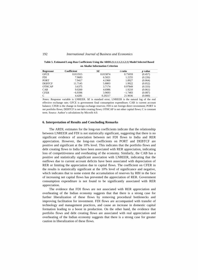
Table 4. Estimated Long-Run Coefficients Using the ARDL(2,0,0,0,0,0,0,0) Model Selected Based

on Schwarz Bayesian Criterion





term. Source: Author’s calculations by Microfit 4.0.


GFCE −0.0098815 0.0072372 −1.3654 (0.178)

FDI 0.070920 3.3836 0.20960 (0.835)

PORT 3.5873 1.9734 1.8178 (0.074)

DEBTCF 5.9138 2.7542 2.1472 (0.036)

OTHCAP 0.17547 2.0551 0.085381 (0.932)

CAB 4.1563 2.0220 2.0556 (0.044) CFER −3.1848 1.6935 −1.8806 (0.065)

C 4.7145 0.098941 47.6498 (0.000)


Table 5. Estimated Long-Run Coefficients Using the ARDL(1,1,1,1,2,1,2,1) Model Selected Based

on Akaike Information Criterion





term. Source: Author’s calculations by Microfit 4.0.

6. Interpretation of Results and Concluding Remarks

The ARDL estimates for the long-run coefficients indicate that the relationship

between LNREER and FDI is not statistically significant, suggesting that there is no

significant evidence of association between net FDI flows to India and RER

appreciation. However, the long-run coefficients on PORT and DEBTCF are

positive and significant at the 10% level. This indicates that the portfolio flows and

debt creating flows to India have been associated with RER appreciation, indicating

loss of competitiveness and overheating of the economy. Similarly, the CAB has a

positive and statistically significant association with LNREER, indicating that the

outflows due to current account deficits have been associated with depreciation of

RER or limiting the appreciation due to capital flows. The coefficient on CFER in

the results is statistically significant at the 10% level of significance and negative,

which indicates that to some extent the accumulation of reserves by RBI in the face

of increasing net capital flows has prevented the appreciation of RER. Government

consumption expenditure is not found to be significantly associated with RER

appreciation.

The evidence that FDI flows are not associated with RER appreciation and

overheating of the Indian economy suggests that that there is a strong case for

further liberalization of these flows by removing procedural bottlenecks and

improving facilitation for investment. FDI flows are accompanied with transfer of

technology and management practices, and cause an increase in domestic capital

formation leading to a boost in production. On the other hand, the evidence that

portfolio flows and debt creating flows are associated with real appreciation and

overheating of the Indian economy suggests that there is a strong case for greater

caution in liberalization of these flows.


GFCE 0.011915 0.015874 0.75059 (0.457)

FDI 7.9683 6.5021 1.2255 (0.226)

PORT 7.9417 4.1960 1.8927 (0.064) DEBTCF 11.7145 5.8803 1.9922 (0.052)

OTHCAP 3.6375 3.7174 0.97849 (0.333)

CAB 9.0260 4.6986 1.9210 (0.061) CFER −6.9396 3.9693 −1.7483 (0.087)

C 4.4281 0.20217 21.9036 (0.000)


References

Athukorala, P. and S. Rajapatirana, (2003), “Capital Inflows and the Real Exchange

Rate: A Comparative Study of Asia and Latin America,” The World Economy,

26, 613-637.

Bakardzhieva, D., S. B. Naceur, and B. Kamar, (2010), “The Impact of Capital and

Foreign Exchange Flows on the Competitiveness of the Developing Countries,”

IMF Working Paper WP/10/154, International Monetary Fund.

Biswas, S. and B. Dasgupta, (2012), “Real Exchange Rate Response to Inward

Foreign Direct Investment in Liberalized India,” International Journal of

Economics and Management, 6, 321-345.

Calvo, G. A., L. Leiderman, and C. M. Reinhart, (1996), “Inflows of Capital to

Developing Countries in the 1990s,” Journal of Economic Perspectives, 10(2),

123-139.

Combes, J. L., T. Kinda, and P. Plane, (2011), “Capital Flows, Exchange Rate

Flexibility and the Real Exchange Rate,” IMF Working Paper, WP/11/9.

Corden, W. M., (1960), “The Geometric Representation of Policies to Attain

Internal and External Balance,” Review of Economic Studies, 28(1), 1-22.

Corden, W. M. and J. P. Neary, (1982), “Blooming Sector and De-Industrialisation

in a Small Open Economy,” Economic Journal, 92(368), 825-848.

Dickey, D. A. and W. A. Fuller, (1979), “Distributors of the Estimators for

Autoregressive Time Series with a Unit Root,” Journal of American Statistical

Association, 74(366), 427-431.

Dornbusch, R., (1974), “Tariffs and Nontraded Goods,” Journal of International

Economics, 4(2), 177-185.

Elbadawi, I. A. and R. Soto, (1994), “Capital Flows and Long-Term Equilibrium

Exchange Rates in Chile,” Policy Research Working Paper 1306, The World

Bank.

Engle, R. F. and C. W. J. Granger, (1987), “Co-Integration and Error Correction:

Representation, Estimation and Testing,” Econometrica, 55(2), 251-276.

Gaiha, A., P. Padhi, and A. Ramanathan, (2014), “An Empirical Investigation of

Causality from Capital Flows to Exchange Rate in India,” International

Journal of Social Sciences and Entrepreneurship, 1, 1-10.

Goel, S. and V. R. Saradhi, (2014), “An Empirical Analysis of the Relationship

between Capital Flows and the Real Exchange Rate in India,” International

Journal of Applied Management and Technology, Walden University, 13, 68-

81.

Javorick, B. S., (2004), “Does Foreign Direct Investment Increase the Productivity

of Domestic Firms? In Search of Spillovers through Backward Linkages,”

American Economic Review, 94(3), 605-627.

Johansen, S. and K. Juselius, (1990), “Maximum Likelihood Estimation and

Inferences on Cointegration—With Applications to the Demand for Money,”

Oxford Bulletin of Economics and Statistics, 52(2), 169-210.

Jongwanich, J. and A. Kohpaiboon, (2013), “Capital Flows and Real Exchange

Rates in Emerging Asian Countries,” Journal of Asian Economics, 24, 138-146.


Lartey, E., (2007), “Capital Inflows and the Real Exchange Rate: An Empirical

Study of Sub-Saharan Africa,” Journal of International Trade & Economic

Development, 16(3), 337-357.

Mejia, L. J., (1999), “Large Capital Flows: A Survey of the Causes, Consequences,

and Policy Response,” IMF Working Paper WP/99/17, International Monetary

Fund.

Pesaran, B. and M. H. Pesaran, (2009), Time Series Econometrics Using Microfit 4.0:

A User’s Manual, New York, NY: Oxford University Press.

Pesaran, M. H. and Y. Shin, (1999), “An Autoregressive Distributed Lag Modeling

Approach to Cointegration Analysis,” S. Strom ed., Econometrics and

Economic Theory in the 20th

Century, The Ragnar Frisch Centennial

Symposium, Cambridge, MA: Cambridge University Press, 371-412.

Pesaran, M. H., Y. Shin, and R. J. Smith, (1996), “Testing for the Existence of a

Long-Run Relationship,” DAE Working Paper, No. 9622, University of

Cambridge.

Pesaran, M. H., Y. Shin, and R. J. Smith, (2001), “Bounds Testing Approaches to

the Analysis of Level Relationships,” Journal of Applied Econometrics, 16(3),

289-236.

Phillips, P. and P. Perron, (1988), “Testing for Unit Root in Time Series Regression,”

Biometrika, 75(2), 335-346.

Reserve Bank of India (RBI), (2005, December), Revision of Nominal Effective

Exchange Rate (NEER) and Real Effective Exchange Rate (REER) Indices,

Bulletin.

Reserve Bank of India (RBI), (2014), Handbook of Statistics,

http://www.rbi.org.in/scripts/AnnualPublications.aspx?head=Handbook%20of

%20Statistics%20on%20Indian%20Economy.

Salter, W. E., (1959), “Internal and External Balance: The Role of Price and

Expenditure Effects,” Economic Record, 35(71), 226-238.

Swan, T. W., (1960), “Economic Control in a Dependent Economy,” Economic

Record, 36(73), 51-66.

capital flow components and the real exchange rate ... of content/pdf/vol14-2/05.pdf · capital...

Documents