CAPITAL- AND LABOR-SAVING

TECHNICAL CHANGE IN AN

AGING ECONOMY

Andreas Irmen∗

University of Luxembourg and CESifo, Munich

Abstract: Does population aging affect economic growth ? The answer is givenin a novel analytical framework that allows for population aging to affect en-dogenous capital- and labor-saving technical change. Population aging is equiv-alent to an increase in the old-age dependency ratio of an OLG-economy withtwo-period lived individuals facing a survival probability. The short-run anal-ysis reveals that population aging induces more labor- and less capital-savingtechnical change as it increases the relative scarcity of labor with respect to cap-ital. Due to external contemporaneous knowledge spill-overs across innovatingfirms induced technical change has a first-order effect on current aggregate in-come. Capital-saving technical change implies that the economy’s steady-stategrowth rate is independent of its age structure: neither a higher life-expectancynor a decline in fertility affects economic growth in the long run.

Keywords: Demographic Transition, Capital Accumulation, Direction of Techni-cal Change.

JEL-Classification: D91, D92, O33, O41.

This Version: January 23, 2013.

∗University of Luxembourg, Faculty of Law, Economics and Finance, 162a, avenue de laFaıencerie, L-1511 Luxembourg, Luxembourg, airmen@uni.lu.A previous version of this paper circulated under the title “Population Aging and the Direction ofTechnical Change”. This research started while I was visiting MIT during the Fall 2008. I wouldlike to thank MIT for its kind hospitality. I am also grateful to Volker Bohm, Hendrik Hakenes,Burkhard Heer, Johanna Kuehnel, Isabel Schnabel, Robert Stelter, Gautam Tripati, Edgar Vogel,Benteng Zou, audiences at Antwerp, Mannheim, Frankfurt, Hannover, Heidelberg, Luxembourg,Stockholm, Vielsalm and Mainz for helpful comments. Finally, I would like to thank DeborahSchwartz and Amer Tabakovic for competent research assistance.

1 Introduction

Does population aging affect economic growth ? Currently, this question is at theheart of many policy debates both in the developing and the developed world.The reason is at least twofold. First, population aging, defined as the process bywhich older individuals become a proportionally larger fraction of the total pop-ulation, has been the predominant demographic phenomenon in many countriesover the last decades and is predicted to reach unprecedented heights. Table 1shows actual data and forecasts of the United Nations concerning the old-agedependency ratio (OADR) for several countries and regions.1 Roughly speak-ing, between 2005 and 2050 the OADR is projected to double in Europe and theUnited States of America. For China, India, Japan and the entire planet its pre-dicted increase is even more pronounced. Second, these developments pose se-rious challenges for many important fields of economic policy including healthcare systems, pension schemes, or public debt (see, e. g., Bloom, Canning, andFink (2008)).

In the political arena economic growth is often seen as a means to solve, or atleast to alleviate, these problems.2 To gauge this prospect it is fundamental tounderstand the causal link between population aging and economic growth. Thisis the topic of the present paper. More precisely, I argue that population aginghas an effect on the investment behavior of firms. These investments are a crucialdeterminant of the speed of technical progress and, eventually, of the growthperformance of an economy.

I address this issue in a novel endogenous growth model that allows for techni-cal change to be capital- and labor-saving. Arguably, allowing for capital-savingtechnical change is the major contribution to the existing literature. This fea-ture turns out to substantially modify the predicted effect of population aging oneconomic growth. The production side of the economy builds on and extendsideas of the so-called ‘induced innovations’ literature (see, e. g., Hicks (1932) andDrandakis and Phelps (1966)). Population aging affects the relative scarcity of la-bor with respect to capital, relative factor prices, and induces technical change.3

1The predictions appear in United Nations (2011) as the ‘medium variant’. The old-age de-pendency ratio is the ratio of the population aged 65 or over to the population aged 15-64. Thisratio is stated as the number of dependants per 100 persons of working age (15-64). I focus onthe OADR as an indicator of population aging since this measure has a natural counterpart in thetheoretical analysis that follows.

2See, e. g., Chancellor Merkel’s government declaration of November 10, 2009 (Merkel (2009)).

3This chain of reasoning connects the phenomenon of population aging to the famous con-

1

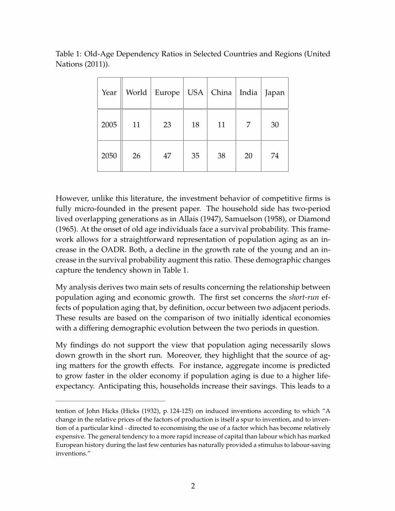
Table 1: Old-Age Dependency Ratios in Selected Countries and Regions (UnitedNations (2011)).

Year World Europe USA China India Japan

2005 11 23 18 11 7 30

2050 26 47 35 38 20 74

However, unlike this literature, the investment behavior of competitive firms isfully micro-founded in the present paper. The household side has two-periodlived overlapping generations as in Allais (1947), Samuelson (1958), or Diamond(1965). At the onset of old age individuals face a survival probability. This frame-work allows for a straightforward representation of population aging as an in-crease in the OADR. Both, a decline in the growth rate of the young and an in-crease in the survival probability augment this ratio. These demographic changescapture the tendency shown in Table 1.

My analysis derives two main sets of results concerning the relationship betweenpopulation aging and economic growth. The first set concerns the short-run ef-fects of population aging that, by definition, occur between two adjacent periods.These results are based on the comparison of two initially identical economieswith a differing demographic evolution between the two periods in question.

My findings do not support the view that population aging necessarily slowsdown growth in the short run. Moreover, they highlight that the source of ag-ing matters for the growth effects. For instance, aggregate income is predictedto grow faster in the older economy if population aging is due to a higher life-expectancy. Anticipating this, households increase their savings. This leads to a

tention of John Hicks (Hicks (1932), p. 124-125) on induced inventions according to which “Achange in the relative prices of the factors of production is itself a spur to invention, and to inven-tion of a particular kind - directed to economising the use of a factor which has become relativelyexpensive. The general tendency to a more rapid increase of capital than labour which has markedEuropean history during the last few centuries has naturally provided a stimulus to labour-savinginventions.”

2

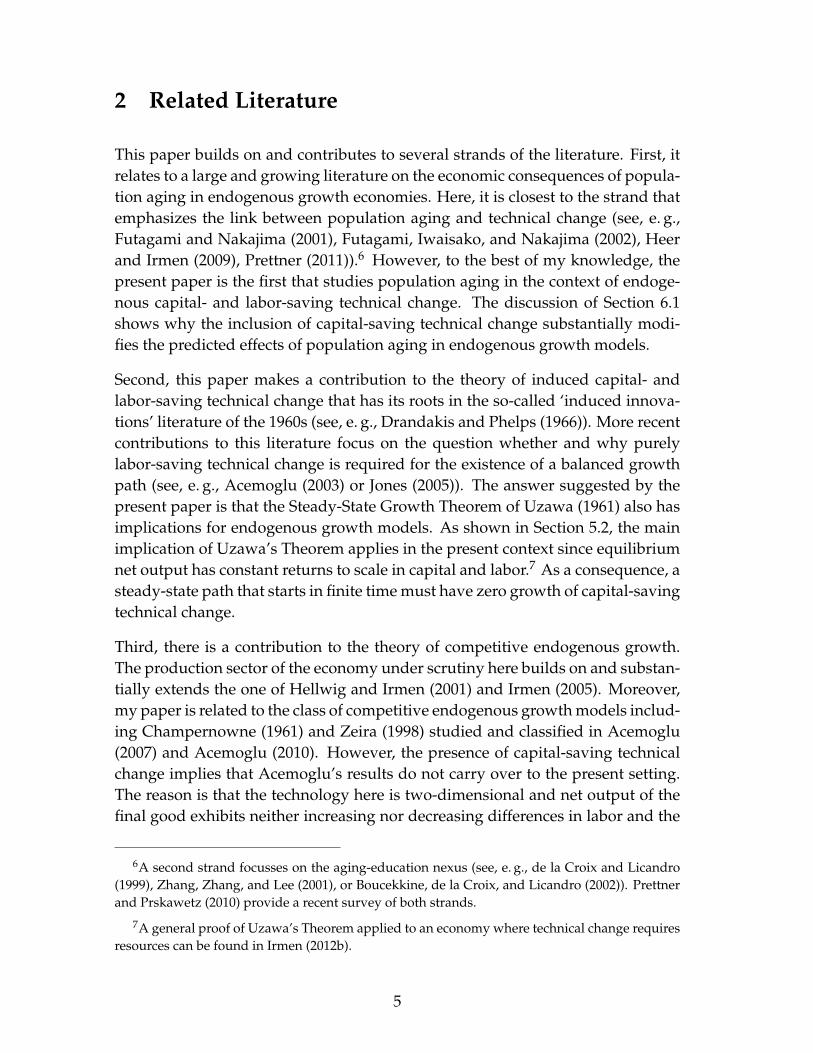
Figure 1.1: Old-Age Dependency Ratio (OADR) and Annual Growth Rates ofPer-capita GDP and GDP per Person Employed: US, 1960-2010.

larger capital stock and induces faster labor productivity growth. Both channelsincrease aggregate income. These forces also drive per-capita income growth.However, their impact is mitigated in the older economy since a higher life-expectancy increases total population.

The second set of results is related to the long-run effects of population aging. As amain finding, I establish that the steady-state growth rate of the economy is inde-pendent of population aging. This property is due to the presence of endogenouscapital-saving technical change. It implies that a variant of Uzawa’s Steady-StateGrowth Theorem (Uzawa (1961)) applies to the economy. Therefore, in the steadystate, capital-saving technical progress vanishes and the growth rate of per-capitavariables is equal to the growth rate of labor-saving technical change. To supportthese growth rates, the state variables of the dynamical system adjust such thatthe investment behavior of profit-maximizing firms is consistent with it. Theseadjustments are shown to be independent of the demographic environment.

There are at least two ways to link these findings to the recent experience of theUS economy. First, as shown in Figure 1.1 for the time span between 1960 and2010, the evolution of the OADR, of per-capita GDP growth, and of labor pro-

3

ductivity growth appear uncorrelated.4 This is the predicted effect of popula-tion aging on steady-state growth. Second, as shown by Klump, McAdam, andWillman (2007) for the period 1953 to 1998, the US economy exhibited exponen-tial labor-saving technical change whereas capital-saving technical change fadedaway. This is the predicted behavior of technical change in the neighborhood ofthe steady state.5

This paper is organized as follows. Section 2 discusses the link to the existingliterature. Section 3 presents the details of the model. Section 4 studies the inter-temporal general equilibrium and establishes the dynamical system. Section 5contains the main results of this paper on the short-run and the long-run implica-tions of population aging for economic growth. Additional results are derived inSection 6. In Section 6.1, I revisit the role of capital-saving technical change andidentify this form of technical change as the main reason for why steady-stategrowth is independent of population aging. The following sections allow for var-ious new features. They highlight the robustness of my results for the long-runand discuss necessary modifications for the short-run analysis. Section 6.2 showsthat all qualitative results remain valid if capital-saving investments generate ex-ternal contemporaneous knowledge spill-overs in the spirit of Frankel (1962) andRomer (1986). Section 6.3 allows for three generations to be alive in each periodand for expectations of survival rates to be myopic. Section 6.4 endogenizes thesupply of labor, Section 6.5 sketches the role of endogenous fertility. Section 7concludes. Proofs are relegated to Appendix A.

4In Figure 1.1 the old-age dependency ratio (OADR) is the ratio of the population aged 65and older per 100 persons of the working-age population aged 15-64. GDP per capita is grossdomestic product divided by midyear population. Data on these variables are from The WorldBank (2012). Data on GDP per person employed is taken from European Commission - Economicand Financial Affairs - AMECO (2012). The impression of zero correlation is confirmed when per-capita GDP or GDP per person employed is regressed on the OADR and a time trend. Then, theimpact of the OADR on the outcome is statistically not different from zero. The p-value in bothregressions is larger than 0.6. The detailed regression results are available from the author uponrequest.

5To the extent that population aging is due to a decline in population growth my results forthe long run support what Bloom, Canning, and Sevilla (2003) call the “neutralist view”: popula-tion aging has no effect on economic growth. These authors support the neutralist view with theassessment that cross-country evidence provides little evidence for population growth to eitherfoster or hamper economic growth (ibidem, p. 17). In their empirical studyAcemoglu and Johnson(2007) find a negative but small causal effect an increased life-expectancy on economic growth.Ashraf, Lester, and Weil (2009) confirm these findings in a simulation exercise. Overall, the em-pirical literature provides mixed results on the effect of life expectancy on economic growth (see,e. g., Bloom, Canning, and Sevilla (2004), Lorentzen, McMillan, and Wacziarg (2008), Cervellatiand Sunde (2011)).

4

2 Related Literature

This paper builds on and contributes to several strands of the literature. First, itrelates to a large and growing literature on the economic consequences of popula-tion aging in endogenous growth economies. Here, it is closest to the strand thatemphasizes the link between population aging and technical change (see, e. g.,Futagami and Nakajima (2001), Futagami, Iwaisako, and Nakajima (2002), Heerand Irmen (2009), Prettner (2011)).6 However, to the best of my knowledge, thepresent paper is the first that studies population aging in the context of endoge-nous capital- and labor-saving technical change. The discussion of Section 6.1shows why the inclusion of capital-saving technical change substantially modi-fies the predicted effects of population aging in endogenous growth models.

Second, this paper makes a contribution to the theory of induced capital- andlabor-saving technical change that has its roots in the so-called ‘induced innova-tions’ literature of the 1960s (see, e. g., Drandakis and Phelps (1966)). More recentcontributions to this literature focus on the question whether and why purelylabor-saving technical change is required for the existence of a balanced growthpath (see, e. g., Acemoglu (2003) or Jones (2005)). The answer suggested by thepresent paper is that the Steady-State Growth Theorem of Uzawa (1961) also hasimplications for endogenous growth models. As shown in Section 5.2, the mainimplication of Uzawa’s Theorem applies in the present context since equilibriumnet output has constant returns to scale in capital and labor.7 As a consequence, asteady-state path that starts in finite time must have zero growth of capital-savingtechnical change.

Third, there is a contribution to the theory of competitive endogenous growth.The production sector of the economy under scrutiny here builds on and substan-tially extends the one of Hellwig and Irmen (2001) and Irmen (2005). Moreover,my paper is related to the class of competitive endogenous growth models includ-ing Champernowne (1961) and Zeira (1998) studied and classified in Acemoglu(2007) and Acemoglu (2010). However, the presence of capital-saving technicalchange implies that Acemoglu’s results do not carry over to the present setting.The reason is that the technology here is two-dimensional and net output of thefinal good exhibits neither increasing nor decreasing differences in labor and the

6A second strand focusses on the aging-education nexus (see, e. g., de la Croix and Licandro(1999), Zhang, Zhang, and Lee (2001), or Boucekkine, de la Croix, and Licandro (2002)). Prettnerand Prskawetz (2010) provide a recent survey of both strands.

7A general proof of Uzawa’s Theorem applied to an economy where technical change requiresresources can be found in Irmen (2012b).

5

vector of technologies. Therefore, in the taxonomy of Acemoglu, the technologyis neither strongly labor saving nor strongly capital-saving.

Finally, this paper also broadens and complements the theory of OLG–models(de la Croix and Michel (2002)). Indeed, I show in Section 4.2 that the dynamicalsystem with endogenous capital- and labor-saving technical change nests sev-eral other specifications. They include the economy where endogenous technicalchange must be labor-saving and the model of Diamond (1965), either with orwithout exogenous technical change.

3 The Basic Model

The economy has a household sector and a final-good sector in an infinite se-quence of periods t = 1, 2, ..., ∞. The household sector comprises two-periodlived individuals facing a survival probability. There are three objects of ex-change. The manufactured final good can be consumed or invested. If invested itmay either become future capital or serve as an input in current capital- or labor-saving investments. Households supply labor and capital. Labor is ‘owned’ bythe young, the old own the capital stock. Capital is the only asset in the economyand, without loss of generality, fully depreciates after one period.8 Each periodhas markets for all three objects of exchange. The final good serves as numeraire.

3.1 Households

Individuals live for possibly two periods, young and old age. When young, theywork, consume, and save. At the onset of old age, they face a survival probabilityν ∈ (0, 1). Survivors retire and consume their wealth. The population at t consistsof Lt young and νLt−1 old individuals. Due to births and other demographicfactors, the amount of young individuals between two adjacent periods grows atrate λ > (−1). For short, I shall refer to λ as the fertility rate.

8My setup is mute on the question as to who owns the infinitely-lived firms in the economy.As individual preferences are defined over the single consumption good of each period, prop-erty rights of firms do not matter for the equilibrium allocation. Moreover, I consider competitiveequilibria where maximized per-period profits are zero such that the expected present discountedvalue of dividends associated with any ownership share is zero, too. It is well known that theseconsiderations are not sufficient to exclude equilibria with bubbles since the number of potentialtraders is infinite in the OLG-framework (Tirole (1985)). In what follows, I disregard this possi-bility and focus on equilibria without bubbles.

6

Young individuals are endowed with a labor endowment equal to unity. It isinelastically supplied to the labor market. Hence, Lt is the labor supply at t andλ its growth rate. The OADR at t is then

OADRt ≡νLt−1

Lt=

ν

1 + λ. (3.1)

According to this measure, there is population aging between period t− 1 and t ifOADRt > OADRt−1. A decline in the fertility rate of generation t− 1 and/or anincrease in the survival probability of this generation leads to population aging.

Preferences of a member of cohort t are homothetic and defined over the level ofconsumption when young and old, cy

t and cot+1, respectively. Normalizing u(0) =

0 to be the utility after death, expected lifetime utility is

Ut = u(cy

t)+ νu

(co

t+1)

, (3.2)

where u : R+ → R is a per-period utility function. It is C2 on R++ and satisfiesu′(c) > 0 > u′′(c) as well as limc→0 u′(c) = ∞.

I follow, e. g., Yaari (1965) or Blanchard (1985), and assume a perfect annuity mar-ket for insurance against survival risk. At the end of their young age, individualsof cohort t deposit their entire savings with mutual funds. These funds rent sav-ings out as capital to the firms producing in t + 1. The latter pay a real rental rateRt+1 per unit of capital. Perfect competition among mutual funds assures a grossreturn to a surviving old at t + 1 of Rt+1/ν.

Hence, the maximization of (3.2) is subject to the per-period budget constraintscy

t + st ≤ wt and cot+1 ≤ st Rt+1/ν, where st denotes savings and wt the real wage

at t. Given the vector of prices, (wt, Rt+1) ∈ R2++, standard arguments reveal that

the optimal plan of a member of cohort t,(cy

t , st, cot+1), includes a continuous and

partially differentiable function9

st = s (Rt+1, ν)wt, with sR (Rt+1, ν) R 0 and sν (Rt+1, ν) > 0. (3.3)

3.2 Firms

At all t, the production sector has a continuum [0, 1] of competitive firms. Withoutloss of generality, their behavior may be analyzed through the lens of a compet-itive representative firm. To save on heavy notation, I shall use this perspectivethroughout the analysis if not indicated otherwise.

9See, e. g., Bloom, Canning, and Graham (2003) for empirical support for the positive effect oflongevity on the savings rate. These authors also find that the effect of the interest rate on thesavings rate is small.

7

3.2.1 Technology

Two types of tasks have to be performed to produce output. The first type needscapital, the second labor as the only input. Let m ∈ R+ index a task performed bycapital and n ∈ R+ a task performed by labor. With mt and nt denoting the total‘number’ of tasks of each type performed at t, I have m ∈ [0, mt] and n ∈ [0, nt].The production function F : R2

+ → R+ assigns the maximum output, Yt, to eachpair (mt, nt) ∈ R2

+, i. e.,

Yt = F (mt, nt) . (3.4)

The function F is C2 on R2++ with F1 > 0 > F11 and F2 > 0 > F22. Moreover,

it exhibits constant-returns-to-scale with respect to both task types.10 For furtherreference, let κt denote the period-t task intensity of the firm, i. e.,

κt =mt

nt. (3.5)

The production function in intensive form is then F (κt, 1) ≡ f (κt), where f :R+ → R+, with f ′ (κt) > 0 > f ′′ (κt) for all κt > 0.

At t, a task m requires kt(m) = 1/bt(m) units of capital, a task n needs lt(n) =

1/at(n) units of labor. Hence, bt(m) and at(n) denote the productivity of capitaland labor, respectively. They are equal to

bt(m) = Bt−1(1− δ)(1 + qBt (m)),

(3.6)

at(n) = At−1 (1− δ)(

1 + qAt (n) + ηAeA

t

);

here Bt−1 and At−1 denote aggregate indicators of the level of technological knowl-edge at t− 1, and δ ∈ (0, 1) is the rate of depreciation of technological knowledgebetween any pair of periods t− 1 and t. Accordingly, the terms Bt−1(1− δ) andAt−1(1− δ) represent the level of technological knowledge to which the firm att has access for free. Then, qB

t (m) ∈ R+ and qAt (n) ∈ R+ are indicators of pro-

ductivity growth associated with task m and task n, respectively. Finally, theproductivity of labor in task n hinges on an external effect, eA

t ≥ 0. It capturesexternal contemporaneous knowledge spill-overs associated with the creation oflabor-saving technical change. This externality is equal to the average productiv-ity growth rates achieved in all tasks using labor, i. e.,

eAt ≡

1nt

∫ nt

0qA

t (n)dn.

10To include, e. g., the CES production function, I make no assumptions on the limits of thefunction F and its derivatives for mt → 0, nt → 0, mt → ∞, and nt → ∞.

8

The parameter ηA ∈ R+ measures its strength.

To achieve productivity growth rates qBt (m) > 0 and qA

t (n) > 0, the firm mustinvest i(qB

t (m)) > 0 and i(qAt (n)) > 0 units of final output in period t. To fix

ideas, suppose that a task has to be performed by a mainframe computer that ispart of a firm’s capital stock. Then, any equipment investment that reduces thetime this computer needs to accomplish the task in question generates capital-saving technical change. Similarly, for a task performed by labor, one may thinkof labor-saving technical change as the result of an equipment investment thatreduces the amount of time a worker needs to accomplish the considered task.11

In addition, labor-saving technical change may also reflect investments of thefirm in the human capital of its workforce. As, e. g., in Lucas (1988), the creationof human capital motivates the presence of the positive external effect wheneverηA > 0.

The function i : R+ → R+ is the same for all tasks, time invariant, C2 on R++,increasing and strictly convex. Hence, higher rates of productivity growth requireever larger investments. Moreover, with the notation i′

(qj) ≡ di

(qj) /dqj for

j = A, B, it satisfies

i(0) = 0, limqj→0

i′(qj) = 0, and limqj→∞

i(

qj)= lim

qj→∞i′(

qj)= ∞. (3.7)

At the level of the individual firm, I assume that any new piece of technolog-ical knowledge is proprietary knowledge of an investing firm only in t, i. e.,in the period when it occurs. Subsequently, the advancement of technologicalknowledge becomes embodied in aggregate task specific productivity indicators(At, Bt), (At+1, Bt+1) , ..., with no further scope for proprietary exploitation. Theevolution of these indicators will be specified below. If the firm decides not tomake an investment for a task m or n then it has access to the production tech-nique represented by At−1(1− δ) and Bt−1(1− δ) such that at(n) = At−1(1− δ)

and bt(m) = Bt−1(1− δ).

11At the semantic level, the effect of technical change associated with equipment investmentsmotivates the terminology ‘capital-saving’ and ‘labor-saving’. Hicks (1932), p. 121-122, classifiedtechnical change according to its effect on the ratio of the marginal product of capital to that oflabor and called technical change labor-saving (capital-saving) if it increases (decreases) this ratio.The results established Irmen (2012a) show that the Hicksian definition applies to the presentmodel, too.

9

3.2.2 Profit-Maximization

The firm takes the sequence {wt, Rt, At−1, Bt−1, eAt }∞

t=1 of real wages, real rentalrates of capital, of aggregate productivity indicators, and of the knowledge exter-nality as given and chooses a production plan

(mt, nt, kt(m), lt(n), qB

t (m), qAt (n)

)for m ∈ [0, mt], n ∈ [0, nt] and all t. This plan maximizes the sum of the presentdiscounted values of profits in all periods. Since an investment generates pro-prietary knowledge only in the period when it is made, the inter-temporal max-imization boils down to the maximization of per-period profits. Hence, for eachperiod t, the firm needs to find the plan that maximizes turnover minus total costs

Πt = F (mt, nt)− Ct,

(3.8)

Ct =∫ mt

0

[Rtkt(m) + i(qB

t (m))]

dm +∫ nt

0

[wtlt(n) + i(qA

t (n))]

dn;

here, Ct sums up the costs per task of both task types. With (3.6) I have

kt(m) =1

Bt−1(1− δ)(1 + qBt (m))

and lt(n) =1

At−1 (1− δ)(1 + qA

t (n) + ηAeAt) .

Therefore, at all t = 1, 2, ..., ∞, the firm’s problem may be split up in two parts.First, it chooses for each n ∈ [0, nt] and m ∈ [0, mt] the values

(qA

t (n), qBt (m)

)∈

R2+ that minimize Ct. Second, it determines the number of tasks (nt, mt) ∈ R2

+

that maximize Πt. The respective first-order (sufficient) conditions for an interiorsolution are12

12Sufficiency follows since Πt is strictly concave in(qA

t (n), qBt (m)

)and exhibits constant returns

to scale in (nt, mt).

10

qAt (n) :

−wt

At−1(1− δ)(1 + qAt (n) + ηAeA

t )2+ i′

(qA

t (n))= 0, ∀n ∈ [0, nt],(3.9)

qBt (m) :

−Rt

Bt−1(1− δ)(1 + qBt (m))2

+ i′(

qBt (m)

)= 0, ∀m ∈ [0, mt], (3.10)

nt : f (κt)− κt f ′ (κt)− i(

qAt (nt)

)− wt

at(nt)= 0, (3.11)

mt : f ′ (κt)− i(

qBt (mt)

)− Rt

bt(mt)= 0. (3.12)

For each task of the respective type, conditions (3.9) and (3.10) equate the marginalreduction of the firm’s wage bill/capital cost to the marginal increase in its invest-ment costs. Hence, these conditions assure that each task is performed at mini-mum cost. Assuming wt > 0 and Rt > 0, the convexity of the innovation costfunction and the fact that limqj→0 i′(qj) = 0, j = A, B, imply that these conditionsdetermine a unique qA

t (n) = qAt > 0 and qB

t (m) = qBt > 0 for either task type.

Accordingly, at(n) = at, bt(m) = bt, and eAt = qA

t .13

Conditions (3.11) and (3.12) assure that the number of tasks of each type is chosenoptimally. For the marginal task it must hold that the difference between its valueproduct and its cost vanishes. The former is expressed in terms of the task inten-sity, the latter is the sum of the investment outlays and the wage, respectivelycapital cost of the marginal task.

Observe that Πt has constant returns to scale in (mt, nt) at qAt (n) = qA

t andqB

t (m) = qBt . Therefore, conditions (3.11) and (3.12) leave the number of tasks

undetermined. They will be pinned down by market clearing conditions. For thesame reason, profit-maximization implies zero profits. Combining the first-orderconditions at the optimum delivers the following important result.

Lemma 1 If (3.9) - (3.12) hold at t, then there are maps, gA : R2++ → R++ and

gB : R++ → R++, such that qAt = gA (κt, ηA) and qB

t = gB (κt) satisfy

gAκ (κt, ηA) > 0 > gB

κ (κt) and gAηA(κt, ηA) < 0 for all κt > 0. (3.13)

13Upon dividing (3.9) by (3.10) and rearranging reveals that the incentives to minimize (to-tal) costs constitute an essential part of Hicks’ conjecture quoted in Footnote 3. Indeed, one ob-tains wt/Rt = At−1

(1 +

(1 + ηA) qA

t)2 i′

(qA

t)

/[Bt−1(1 + qB

t )2 i′(qB

t)]

. Since the numerator ofthe right-hand side increases in qA

t and the denominator increases in qBt , an increase in the rela-

tive price of labor induces, ceteris paribus, relatively more labor-saving technical change, i. e., ahike in wt/Rt means a greater ratio qA

t /qBt .

11

Figure 3.1: The Link between κt, qAt = gA (κt, ηA) and wt.

Moreover, there are maps w : R2++ → R++ and R : R2

++ → R++, such that the realwage and the rental rate of capital satisfy

wt = w(κt, At−1) > 0, with wκ(κt, At−1) > 0, wA(κt, At−1) > 0,

(3.14)

Rt = R(κt, Bt−1) > 0, with Rκ(κt, Bt−1) < 0, RB(κt, Bt−1) > 0.

Lemma 1 states two key properties of the production sector. First, the equilibriumincentives to engage in labor- and capital-saving technical change depend on thetask intensity. The incentive to engage in labor-saving technical change increaseswith this intensity, the incentive to engage in capital-saving technical change de-creases with it. Moreover, the positive externality reduces the incentives to investin labor-saving technical change. Second, factor prices may be expressed as afunction of the task intensity and the respective technology indicators, At−1 andBt−1.14 While the real wage increases with the task intensity, the real rental rate ofcapital declines with it. Both factor prices increase in the technology indicators.

Intuitively, the effect of changing κt on investment incentives and factor prices re-flects two sides of the same coin. To see this, consider a triple

(κt, gA (κt, ηA) , wt

)14One readily verifies that the function w also depends on ηA with wηA being indeterminate in

general. Since this argument is of little interest for what follows I shall suppress it.

12

that satisfies (3.9) and (3.11). As shown in Figure 3.1, for these values the costper task is minimized (right panel) and this minimum is equal to the marginalvalue product of task nt (left panel). The latter increases as κt increases to κ′t sothat the minimum cost of task nt must increase. This requires the higher wagew′t, hence wκ(κt, At−1) > 0. At w′t, the marginal benefit of faster productivitygrowth is higher. Therefore, the minimum cost is attained at a higher qA

t , hencegA

κ (κt, ηA) > 0. The effect of κt on Rt and qBt may be derived in an analogous

manner. However, in this case an increase in κt reduces the marginal value prod-uct of task mt in (3.12). Therefore Rt must decline, and so does qB

t in accordancewith (3.10). Hence, Rκ(κt, Bt−1) < 0 and gB

κ (κt) < 0.

Finally, note that the external effect increases in ηA. Therefore, a larger ηA weak-ens the marginal cost advantage of labor-saving innovation investments. Accord-ingly, the cost per task reaches its minimum at a lower level of qA

t . This explainswhy gA

ηA(κt, ηA) < 0.

3.3 The Evolution of Technological Knowledge

The evolution of the economy’s level of technological knowledge is given by theevolution of the aggregate task specific productivity indicators At and Bt. Animportant question is then how these indicators are linked to the productivityenhancing investments associated with all performed tasks. In what follows Iassociate the highest level of labor and capital productivity attained across alltasks of a respective type with At and Bt, i. e.,

At = max{at(n) = At−1(1− δ)(

1 + qAt (n) + ηAeA

t

)| n ∈ [0, nt]}

(3.15)

Bt = max{bt(m) = Bt−1(1− δ)(

1 + qBt (m)

)|m ∈ [0, mt]}.

Since profit-maximization implies qAt (n) = qA

t = eAt , qB

t (m) = qBt , at(n) = at, and

bt(m) = bt, I have

At = at = At−1(1− δ)(

1 +(

1 + ηA)

qAt

)(3.16)

Bt = bt = Bt−1(1− δ)(

1 + qBt

)for all t = 1, 2, ..., ∞, with A0 > 0 and B0 > 0 as initial conditions.

13

4 Inter-temporal General Equilibrium

4.1 Definition

A price system corresponds to a sequence {wt, Rt}∞t=1. An allocation is a sequence

{cyt , st, co

t , Yt, nt, mt, qAt (n), qB

t (m), at(n), bt(m), lt(n), kt(m), eAt , Lt, Kt}∞

t=1

for all tasks n ∈ [0, nt] and m ∈ [0, mt]. It comprises a strategy {cyt , st, co

t+1}∞t=1 for

all cohorts, consumption of the old at t = 1, co1, and a strategy for the production

sector {Yt, nt, mt, qAt (n), qB

t (m), at(n), bt(m), lt(n), kt(m)}∞t=1.

For an exogenous evolution of the labor force, Lt = L1 (1 + λ)t−1 with L1 > 0 andλ > (−1), a given survival probability ν for all cohorts t = 2, 3, ..., ∞, a given ini-tial level of capital, K1 > 0, and initial values of technological knowledge, A0 > 0and B0 > 0, an inter-temporal general equilibrium with perfect foresight correspondsto a price system, an allocation, and a sequence {At, Bt}∞

t=1 of aggregate produc-tivity indicators that satisfy the following conditions for all t = 1, 2, ..., ∞:

(E1) The young of each period save according to (3.3) and supply Lt units of labor.

(E2) The production sector satisfies Lemma 1.

(E3) The market for the final good clears, i. e.,

Lt−1cot + Ltc

yt + IK

t + IAt + IB

t = Yt, (4.1)

where IKt is aggregate capital investment, IA

t and IBt denote aggregate innovation

investments in labor- and capital-saving technical change.

(E4) There is full employment of labor and capital, i. e.,∫ nt

0lt(n)dn = Lt and

∫ mt

0kt(m)dm = Kt. (4.2)

(E5) The productivity indicators At and Bt evolve according to (3.16).

(E1) guarantees optimal behavior of the household sector under perfect foresight.Since the surviving old own the capital stock, their consumption at t = 1 isν0L0co

1 = R1K1. (E2) assures optimal behavior of the production sector and zeroprofits. (E3) states the resource constraint in (4.1). It reflects the fact that capitalfully depreciates after one period.

14

Full employment of labor and capital, i. e., (E4), and Lemma 1 imply that in equi-librium

nt = atLt and mt = btKt, (4.3)

IAt = atLti

(qA

t

)and IB

t = btKti(

qBt

), (4.4)

i. e., for each task type the number of performed tasks is equal to the respective in-put in efficiency units. In other words, technical change is factor augmenting andYt = F (btKt, atLt). Moreover, aggregate investment in labor- and capital-savingtechnical change is proportionate to the respective input in efficiency units.

Observe that the task intensity of (3.5) and the full employment condition (4.3)imply that κt = mt/nt = btKt/atLt. Hence, in equilibrium the task intensity isequal to the ‘efficient capital intensity’ defined as the amount of efficient capitalper unit of efficient labor. However, from Lemma 1 the efficient capital intensityitself depends on the task intensity, i. e.,

κt =Bt−1

(1 + gB (κt)

)Kt

At−1 (1 + (1 + ηA) gA (κt, ηA)) Lt. (4.5)

Therefore, I have to make sure that a value κt > 0 exists that satisfies (4.5). Toaddress this issue, denote by

εAκ

(κt, ηA

)≡

d ln(1 +

(1 + ηA) gA (κt, ηA))

d ln κt> 0, εB

κ (κt) ≡−d ln

(1 + gB (κt)

)d ln κt

> 0

the elasticities of the respective productivity growth factors with respect to theefficient capital intensity.

Lemma 2 There is a map κ : R++ → R++ such that

κt = κ

(Bt−1Kt

At−1Lt

)> 0 (4.6)

satisfies (4.5). Moreover,

εκ(κt) ≡d ln κt

d ln (Kt/Lt)=

11 + εA

κ (κt, ηA) + εBκ (κt)

∈ (0, 1). (4.7)

Hence, there is a unique solution κt > 0 to (4.5).15 Moreover, an increase inthe capital-labor ratio, Kt/Lt, implies a higher efficient capital intensity. Due toinduced innovation investments, this increase is less than proportionate.

15For ease of notation, the dependency of the functions κ(·) and εκ(·) from ηA is suppressed.

15

4.2 The Dynamical System

The equilibrium conditions (E1) - (E5) require savings to equal capital investment,i. e.,

IKt = stLt = Kt+1, for t = 1, 2, ..., ∞. (4.8)

The evolution of the economy may then be characterized by means of two statevariables, namely the efficient capital intensity, κt, and the level of the aggregateproductivity indicator Bt. Let w (κt) ≡ w(κt, At−1)/at denote the real wage perefficiency unit. Moreover, use (3.3), (3.14), and (4.5) to define the elasticities

εsR(κt) ≡

d ln s (R (κt, Bt−1) , ν)

d ln RtR 0, and εR

κ (κt) ≡d ln R(κt, Bt−1)

d ln κt< 0.

With ε (κt+1) ≡ [εsR (κt+1)]

[εR

κ (κt+1)][εκ (κt+1)], the dynamical system may be

stated as follows.

Proposition 1 Given (K1, L1, A0, B0) > 0 as initial conditions, there is a unique equi-librium sequence {κt, Bt}∞

t=1 determined by

s (R (κt+1, Bt) , ν)

1 + λw (κt) =

κt+1

Bt

1 +(1 + ηA) gA (κt+1, ηA)

1 + gB (κt+1), (4.9)

and

Bt = Bt−1 (1− δ)(

1 + gB (κt))

, (4.10)

if

ε (κt+1) < 1 for all κt+1 > 0. (4.11)

For t = 1, κ1 is given by

κ1 =B0(1 + gB (κ1)

)K1

A0 (1 + (1 + ηA) gA (κ1, ηA)) L1> 0. (4.12)

According to Proposition 1, the dynamical system may be stated as a two-dimensionalsystem of first-order, autonomous, non-linear difference equations. The equationof motion for the efficient capital intensity is (4.9). It restates the condition for sav-ings to equal capital investment, i. e., (4.8), where Kt+1 is replaced by an updateof (4.5). For any given pair (κt, Bt) ∈ R2

++, (4.9) assigns a unique value κt+1 > 0if (4.11) holds. This value of κt+1 is then used to derive Bt+1 from (4.10). SinceK1, L1, A0, and B0 are initial conditions, κ1 is pinned down by (4.5) for t = 1.

16

Observe that the dynamical system of Proposition 1 nests several OLG–modelswith either endogenous or exogenous economic growth. For instance, the case ofan economy with only endogenous labor-saving technical change obtains whenqB

t (m) = 0 and Bt = 1 are fixed for all t. I discuss this case in Section 6.1 to furtherelucidate the role of endogenous capital-augmenting technical change. Assum-ing in addition that labor productivity growth is equal to qA > (−1) for all t andcostless, i. e., setting i(qA) = 0, turns the production side into the one of the neo-classical growth model with exogenous labor-saving technical change. Then (4.9)reduces to s (R (κt+1) , ν) w (κt) / (1 + λ) = κt+1

(1 +

(1 + ηA) qA), with κ1 =

K1/[L1A0(1− δ)(1 +

(1 + ηA) qA)

]. If moreover qA = δ/

[(1− δ)

(1 + ηA)],

then (4.9) collapses to Diamond’s difference equation for the capital intensity (Di-amond (1965)).

From this perspective, condition (4.11), which states the permissible percentagechange of the savings rate induced by an increase in Kt+1/Lt+1 at κt+1, may beseen as a generalization of a condition for the existence and the uniqueness of theinter-temporal equilibrium under perfect foresight in an OLG-economy withouttechnical change (see, e. g., de la Croix and Michel (2002), p. 20 ff.). It allows forthe savings rate to decline in response to an increase in the rental rate of capital.However, this decline should not be too pronounced.

5 Population Aging and Economic Growth

Now, I turn to the implications of the preceding results for the relationship be-tween population aging and economic growth. I start with the short-run implica-tions before I turn to the long run.

5.1 Population Aging and Economic Growth in the Short-Run

By definition, the short-run effects of population aging arise if the old-age depen-dency ratio increases between two adjacent periods. Taking the fertility and themortality channel separately, this is either due to a decline in the fertility of theyoung of the first of these periods and/or to an (anticipated) increase in their sur-vival probability. Both demographic changes increase the old-age dependencyratio in the second of the two periods. The following proposition compares theevolution of two initially identical economies that experience differing patternsof population aging between t and t + 1.

17

Proposition 2 Consider two economies with identical initial conditions (Kt, Lt, At−1, Bt−1)

at some period t ≥ 1. If the cohorts t of these economies have different fertility rates, λ >

λ′, and/or different survival probabilities, ν′ > ν, then (Kt+1/Lt+1)′ > Kt+1/Lt+1.

Moreover,(qA

t+1

)′> qA

t+1,(

qBt+1

)′< qB

t+1, w′t+1 > wt+1, and R′t+1 < Rt+1. (5.1)

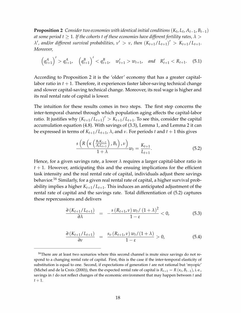
According to Proposition 2 it is the ‘older’ economy that has a greater capital-labor ratio in t + 1. Therefore, it experiences faster labor-saving technical changeand slower capital-saving technical change. Moreover, its real wage is higher andits real rental rate of capital is lower.

The intuition for these results comes in two steps. The first step concerns theinter-temporal channel through which population aging affects the capital-laborratio. It justifies why (Kt+1/Lt+1)

′ > Kt+1/Lt+1. To see this, consider the capitalaccumulation equation (4.8). With savings of (3.3), Lemma 1, and Lemma 2 it canbe expressed in terms of Kt+1/Lt+1, λ, and ν. For periods t and t + 1 this gives

s(

R(

κ(

BtKt+1AtLt+1

), Bt

), ν)

1 + λwt =

Kt+1

Lt+1. (5.2)

Hence, for a given savings rate, a lower λ requires a larger capital-labor ratio int + 1. However, anticipating this and the ensuing implications for the efficienttask intensity and the real rental rate of capital, individuals adjust there savingsbehavior.16 Similarly, for a given real rental rate of capital, a higher survival prob-ability implies a higher Kt+1/Lt+1. This induces an anticipated adjustment of therental rate of capital and the savings rate. Total differentiation of (5.2) capturesthese repercussions and delivers

∂ (Kt+1/Lt+1)

∂λ= − s (Rt+1, ν)wt/ (1 + λ)2

1− ε< 0, (5.3)

∂ (Kt+1/Lt+1)

∂ν=

sv (Rt+1, ν)wt/(1 + λ)

1− ε> 0, (5.4)

16There are at least two scenarios where this second channel is mute since savings do not re-spond to a changing rental rate of capital. First, this is the case if the inter-temporal elasticity ofsubstitution is equal to one. Second, if expectations of generation t are not rational but ‘myopic’(Michel and de la Croix (2000)), then the expected rental rate of capital is Rt+1 = R (κt, Bt−1), i. e.,savings in t do not reflect changes of the economic environment that may happen between t andt + 1.

18

where all elasticities are evaluated at κt+1. The signs follow from (4.11) and sv >

0. Hence, an increase in the OADR induced either by a decline in fertility and/orby an increase in the survival probability leads to a higher capital-labor ratio.

The second step reflects the static adjustments in t+ 1 to an increase in the capital-labor ratio. According to Lemma 2, the (λ′, ν′) – economy exhibits a greater effi-cient capital intensity, i. e., κ′t+1 > κt+1. In accordance with Lemma 1, the latterinduces the technology and price adjustments stated in (5.1).17

What are the implications of Proposition 2 for the growth rate of aggregate andper-capita income? To address this question, let Vt denote aggregate equilibriumincome, or ‘income’ for short. Since Πt = 0 in equilibrium, income is equal tothe difference between the output of the final good and total investment outlays.More precisely, from (3.8), the market-clearing conditions (4.3) and (4.4), I obtain

Vt ≡ V (btKt, atLt) = F (btKt, atLt)− atLti(

qAt

)− btKti

(qB

t

), (5.5)

and per-capita income at t is vt ≡ Vt/ (νLt−1 + Lt).

To prepare for the analysis of how population aging affects income growth, itproves useful to describe how changing factor supplies affect Vt through inducedtechnical change. I denote this effect by EL

t if it is due to a change in the laborforce at t and by EK

t if it is due to a change in the capital stock at t. Using (3.16)and Lemma 1 in (5.5) delivers

ELt =

[∂Vt

∂qAt

gAκ

(κt, ηA

)+

∂Vt

∂qBt

gBκ (κt)

]∂κt

∂Lt,

(5.6)

EKt =

[∂Vt

∂qAt

gAκ

(κt, ηA

)+

∂Vt

∂qBt

gBκ (κt)

]∂κt

∂Kt.

Since gAκ

(κt, ηA) > 0 > gB

κ (κt), changing factor endowments induce technicaladjustments of opposite sign. In spite of this, the following lemma shows thatthese adjustments have unequivocal effects on income.

Lemma 3 In equilibrium, it holds that

∂Vt

∂qAt=

ηAwtLt

1 + (1 + ηA) qAt> 0, and

∂Vt

∂qBt= 0. (5.7)

17Observe that both steps taken together provide a straightforward link between populationaging and Hicks’ contention mentioned in Footnote 3: population aging leads to a higher capital-labor ratio, i. e., the relative scarcity of labor increases. This induces a higher real wage, a lowerreal rental rate, more labor- and less capital-saving technical change.

19

Moreover,

ELt < 0 and EK

t > 0. (5.8)

According to the first result of Lemma 3, a small increase in qAt , evaluated at the

equilibrium, increases Vt, whereas such an increase in qBt leaves Vt unchanged.

The reason for this asymmetry lies in the presence of ηA > 0. Void of a contem-poraneous knowledge externality associated with capital-saving investments, thecompetitive economy chooses the level qB

t that maximizes income, i. e., ∂Vt/∂qBt =

0.18 The positive knowledge externality associated with labor-saving investmentsleads to under-investment in equilibrium. Therefore, having more of qA

t increasesVt at the margin.19

The second result of Lemma 3 uses the reasoning above to conclude from (5.6)that EL

t < 0 and EKt > 0. Hence, both a decline in the labor force and an increase

in the capital stock induce more labor-saving technical change that increases in-come.

The following proposition compares the evolution of aggregate and per-capitaincome between period t and t + 1 in the economies of Proposition 2. Denote theequilibrium income obtained under λ or ν by Vt+1 = V (bt+1Kt+1, at+1Lt+1) andthe one obtained under λ′ or ν′ by V′t+1 = V

(b′t+1K′t+1, a′t+1L′t+1

).

Proposition 3 Consider two economies with identical initial conditions (Kt, Lt, At−1, Bt−1)

at some period t ≥ 1.

18See Irmen (2012a) a for a detailed discussion. Related results appear in the competitiveeconomies studied in Zeira (1998) and Acemoglu (2010).

19To see by how much, a productivity effect and an investment effect of opposite sign must beconsidered. There is a productivity effect since labor becomes more productive. Therefore, moretasks must be performed to satisfy the full employment condition (4.2), nt = At−1(1 − δ)(1 +

(1 + ηA)qAt )Lt. This gives At−1(1− δ)(1 + ηA)Lt additional tasks. As each of these contributes

wtlt = wt/at to income, the productivity effect accounts for At−1(1− δ)(1 + ηA)Ltwt/at addi-tional income.

The investment effect reduces income since for each task already performed, the invest-ment outlays increase by i′(qA

t ). Therefore, total additional investment outlays increase byAt−1(1 − δ)(1 + (1 + ηA)qA

t )Lti′(qAt ). Since firms minimize costs, I have from (3.9) that (1 +

(1 + ηA)qAt )i′(qA

t ) = wt/at. Hence, investment outlays increase by At−1(1− δ)Ltwt/at.The difference between both effects is ηA At−1(1 − δ)Ltwt/at. With (3.16) this is equal to

ηA times economy’s wage bill discounted by the growth factor of labor productivity, i. e.,ηAwtLt/(1 + (1 + ηA)qA

t ).

20

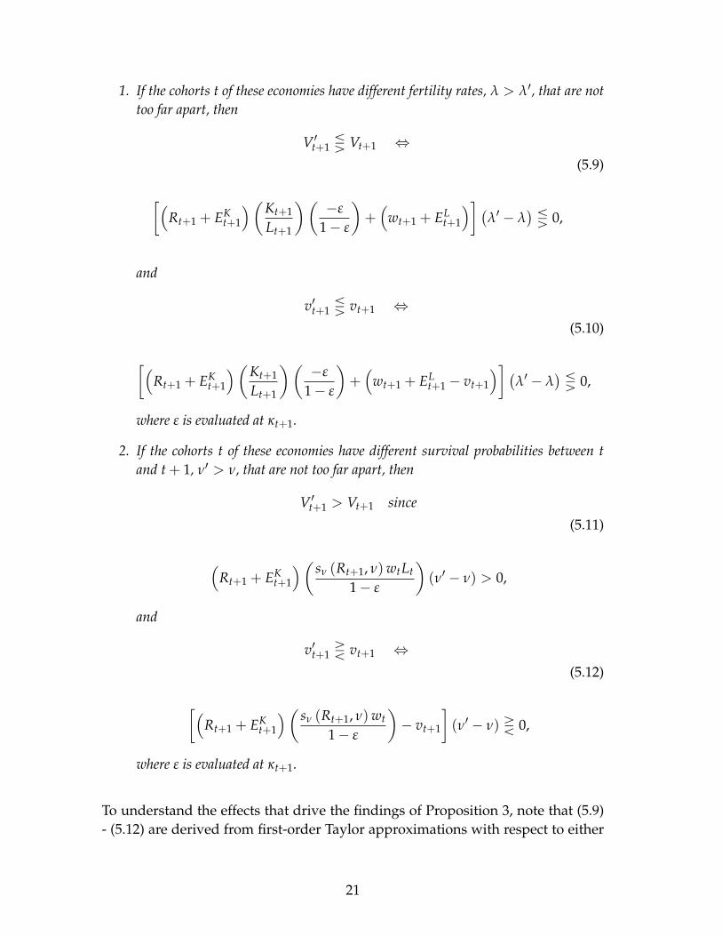
1. If the cohorts t of these economies have different fertility rates, λ > λ′, that are nottoo far apart, then

V′t+1 Q Vt+1 ⇔(5.9)

[(Rt+1 + EK

t+1

)(Kt+1

Lt+1

)(−ε

1− ε

)+(

wt+1 + ELt+1

)] (λ′ − λ

)Q 0,

and

v′t+1 Q vt+1 ⇔(5.10)

[(Rt+1 + EK

t+1

)(Kt+1

Lt+1

)(−ε

1− ε

)+(

wt+1 + ELt+1 − vt+1

)] (λ′ − λ

)Q 0,

where ε is evaluated at κt+1.

2. If the cohorts t of these economies have different survival probabilities between tand t + 1, ν′ > ν, that are not too far apart, then

V′t+1 > Vt+1 since

(5.11)

(Rt+1 + EK

t+1

)( sν (Rt+1, ν)wtLt

1− ε

)(ν′ − ν) > 0,

and

v′t+1 R vt+1 ⇔(5.12)

[(Rt+1 + EK

t+1

)( sν (Rt+1, ν)wt

1− ε

)− vt+1

](ν′ − ν) R 0,

where ε is evaluated at κt+1.

To understand the effects that drive the findings of Proposition 3, note that (5.9)- (5.12) are derived from first-order Taylor approximations with respect to either

21

λ or ν of V′t+1 at Vt+1. This procedure involves two steps. The first step approxi-mates V′t+1 at (Kt+1, Lt+1). This gives

V′t+1 ≈ Vt+1 +dVt+1

dKt+1(K′t+1 − Kt+1) +

dVt+1

dLt+1(L′t+1 − Lt+1). (5.13)

Here, dVt+1/dKt+1 and dVt+1/dLt+1 denote the total effect of changing Kt+1 andLt+1 on Vt+1, respectively. They comprise a direct effect equal to the respectivefactor price and the induced effect of (5.6), i. e.,20

dVt+1

dKt+1=

∂Vt+1

∂Kt+1+ EK

t+1 = Rt+1 + EKt+1 > 0,

(5.14)dVt+1

dLt+1=

∂Vt+1

∂Lt+1+ EL

t+1 = wt+1 + ELt+1 > 0.

Hence, both effects are positive. From Lemma 3, the induced effect associatedwith Kt+1 reinforces the partial effect whereas the induced effect of Lt+1 weakensthe partial effect without dominating it.21

The second step derives first-order Taylor approximations with respect to eitherλ or ν of K′t+1 at Kt+1 to express

(K′t+1 − Kt+1

)in (5.13). Moreover, it uses L′t+1 −

Lt+1 = Lt(λ′ − λ) < 0.

Roughly speaking, the results of (5.9) - (5.12) reveal that the effect of populationaging on the growth rate of aggregate and per-capita income hinges on the signand the strength of the induced effects and on the response of savings. Onlythe effect of a higher survival probability on income growth has an unequivocalpositive sign. This is so since a higher survival probability induces more savings.The resulting higher capital stock contributes positively to output (direct effect)and leads to more labor-saving technical change (induced effect). As shown in(5.12), the effect of life-expectancy on per-capita income is not unequivocal sincemore survivors increase the population in t + 1.

The effect of a decline in fertility is more involved since it triggers both a decline inthe work force and an adjustment of the capital stock. The former channel reducesincome in the λ′ – economy since wt+1 + EL

t+1 > 0. Hence, for V′t+1 < Vt+1, it is

20From (5.5), the direct effect of Kt+1 on Vt+1 is ∂Vt+1/∂Kt+1 = bt+1[F1 (·)− i

(qB

t+1)]

. It has aninterpretation as the marginal contribution of capital to income given qA

t+1 and qBt+1. From (3.12),

it is equal to Rt+1. Similarly, ∂Vt+1/∂Lt+1 = at+1[F2 (·)− i

(qA

t+1)]

is the marginal contributionof labor to income. From (3.11), the latter is equal to wt+1.

21Using Lemma 1 and Lemma 2, one readily verifies that the sign of ∂Vt+1/∂Lt+1 follows sincewt+1

[1−

(ηA/

(1 + ηA)) (εA

κ (κt+1, ηA)/(1 + εA

κ (κt+1, ηA) + εBκ (κt+1)

))]> 0.

22

sufficient to have εsR ≥ 0. Given that the latter is the most likely response of

the savings rate to changes in the rental rate of capital, the prediction is that theλ′ – economy has a lower growth rate of income. However, this does not implythat a lower fertility rate slows down growth of per-capita income. Condition(5.10) highlights that v′t+1 > vt+1 is easier to satisfy since the population at t + 1is smaller under λ′. For instance, if the response of savings to the real rental rateis negligible a decline in fertility increases the growth rate of per-capita income inthe short run if wt+1 + EL

t+1 − vt+1 < 0.

5.2 Population Aging and Economic Growth in the Long-Run

The focus here is on the effects of population aging on economic growth in thesteady state of the dynamical system of Proposition 1. As will become clear below,to derive interpretable results at a high level of generality, I need to impose morestructure. Therefore, I shall strengthen condition (4.11) and henceforth assumethat individuals do not decrease their savings in response to an increase in thereal rental rate of capital, i. e., sR (Rt+1, ν) ≥ 0 or εs

R(κt) ≥ 0.22

Moreover, to study the local stability properties of a steady state let me denotethe two sets {(Bt, κt) |κt+1 − κt = 0} and {(Bt, κt) |Bt+1 − Bt = 0} by ∆κt = 0 and∆Bt = 0, respectively. I assume that the evolution of κt is stable in the vicinity of∆κt = 0. This assumption allows for a meaningful comparison of steady states ina world with and without capital-saving technical change (see, e. g., Section 6.1).

Define a steady state as a trajectory along which all variables grow at a constantrate. I deduce from (4.10) that a trajectory with Bt+1/Bt − 1 = const. requiresκt = κt+1 = κ∗. Moreover, according to (4.9), the latter needs Bt+1 = Bt = B∗.Hence, a steady state is a solution to

s (R (κ∗, B∗) , ν)

1 + λw (κ∗) =

κ∗

B∗(1− δ)

(1 +

(1 + ηA

)gA (κ∗)

). (5.15)

gB (κ∗) =δ

1− δ(5.16)

Proposition 4 (Steady State)

22Without this assumption, neither the existence nor the uniqueness of a steady state may beestablished. Indeed, one readily verifies that, given κ∗, equation (5.15) below may determine noneor several values B∗ > 0 if sR (Rt+1, ν) was allowed to be negative.

23

1. There is a unique steady state involving κ∗ ∈ (0, ∞) and B∗ ∈ (0, ∞) if and onlyif

limκ→0

f ′(κ) >i′ (δ/(1− δ))

1− δ+ i (δ/(1− δ)) > lim

κ→∞f ′(κ). (5.17)

2. The steady-state growth rate of the economy is

g∗ ≡ At+1

At= (1− δ)

(1 + (1 + ηA)gA

(κ∗, ηA

))− 1.

Moreover, along a steady-state path, I have

a)vt+1

vt=

at+1

at=

wt+1

wt=

cyt+1

cyt

=co

t+1co

t=

st+1

st= 1 + g∗,

b)Vt+1

Vt=

Yt+1

Yt=

Kt+1

Kt=

nt+1

nt=

mt+1

mt= (1 + g∗) (1 + λ) ,

c) Bt = bt = B∗, R∗ = B∗i′ (δ/(1− δ))

1− δ, kt = k∗ =

1B∗

,lt+1

lt=

11 + g∗

,

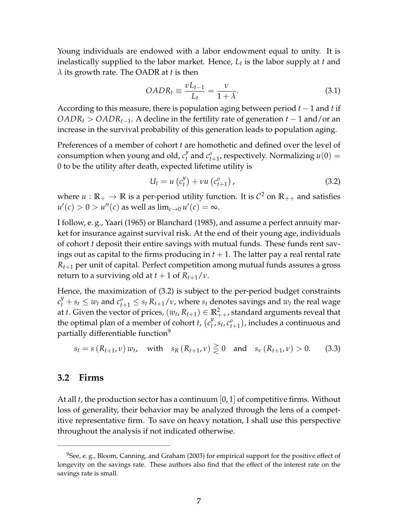
3. If the set ∆κt = 0 is stable in the vicinity of (κ∗, B∗), then the steady state is eithera stable node, a focus, or a clockwise spiral sink. A typical phase diagram looks likethe one of Figure 5.1.

Proposition 4 states important properties of a steady state. According to State-ment 1, a finite and unique steady state exists iff, at the equilibrium allocation,a small (large) stock of efficient capital has a sufficiently high (low) marginalvalue product. This mimics the role of diminishing returns for the existenceof a steady state in the neoclassical growth model of Solow (1956) and Swan(1956). However, here the intuition is quite different. In fact, condition (5.17)assures that qB

t = gB(κt) defined in Lemma 1 may take on the value δ/(1− δ)

for some κ∗ ∈ (0, ∞). For this to be possible the first-order conditions (3.10)and (3.12) has to hold for some mt ∈ (0, ∞) at qB

t = δ/(1 − δ). Then, (3.10)implies that i′(δ/(1− δ))/(1− δ) is equal to the capital cost of task mt so thati′(δ/(1− δ))/(1− δ) + i(δ/(1− δ)) is its total cost. Using the latter in (3.12) re-veals that (5.17) is the desired condition for κ∗ ∈ (0, ∞). Notice that such a valuewould always exist if I had imposed the usual Inada conditions on F.

Statement 2 of Proposition 4 gives the steady-state evolution of all admissiblevariables. The steady-state growth rate of the economy is equal to the growth

24

Figure 5.1: The Phase-Diagram of the Locally Stable Steady State (κ∗, B∗).

rate of the stock of labor-saving technological knowledge. Per-capita income, la-bor productivity, the real wage, and individual consumption and individual sav-ings grow at this rate. Since κ∗ is determined by the production side, an impor-tant conclusion is that the steady-state growth rate is independent of populationaging.23

Aggregate variables such as Yt or Kt grow at rate g∗+λ. Hence, an older economyexperiences slower growth of economy-wide variables. There is no growth ofcapital-saving technological knowledge. Therefore, the rental rate of capital isconstant.24 With these results at hand, it is straightforward to see that the steadystate is consistent with Kaldor’s facts (Kaldor (1961)) as long as g∗ > 0.

The conceptual underpinning of Statement 2 of Proposition 4 is the so-calledSteady-Steady Growth Theorem of Uzawa (Uzawa (1961)). To see this, recall ag-gregate income of (5.5). A steady-state trajectory as defined above for all t ≥

23What then explains different steady-state growth rates in the present model? It is not difficultto show that a higher ηA unequivocally increases g∗ since the (positive) direct effect dominatesthe (negative) indirect effect through gA (κ∗, ηA). Moreover, if I replace the production function(3.4) by Yt = ΓF (mt, nt), where Γ > 0 reflects cross-country differences in geography, technical orsocial infrastructure, then g∗ is strictly increasing in Γ > 0.

24One readily verifies that the steady-state functional income distribution is constant and alsoindependent of population aging.

25

τ ≥ 1 requires qAt = qA and qB

t = qB. Then, Uzawa’s theorem applies sinceV (btKt, atLt) has constant returns to scale in Kt and Lt as well as positive anddiminishing marginal products of Kt and Lt, and IK

t > 0. Hence, bτ = b∗,qB = δ/(1 − δ), and technical progress is only labor-saving. Clearly, technicalprogress is exogenous in Uzawa’s setting. With endogenous capital-saving tech-nical change the efficient capital intensity has to adjust such that firms find itoptimal to invest what is required by the steady-state growth theorem, i. e., theamount that guarantees zero net growth of capital-saving technological knowl-edge. This is guaranteed by (5.16).

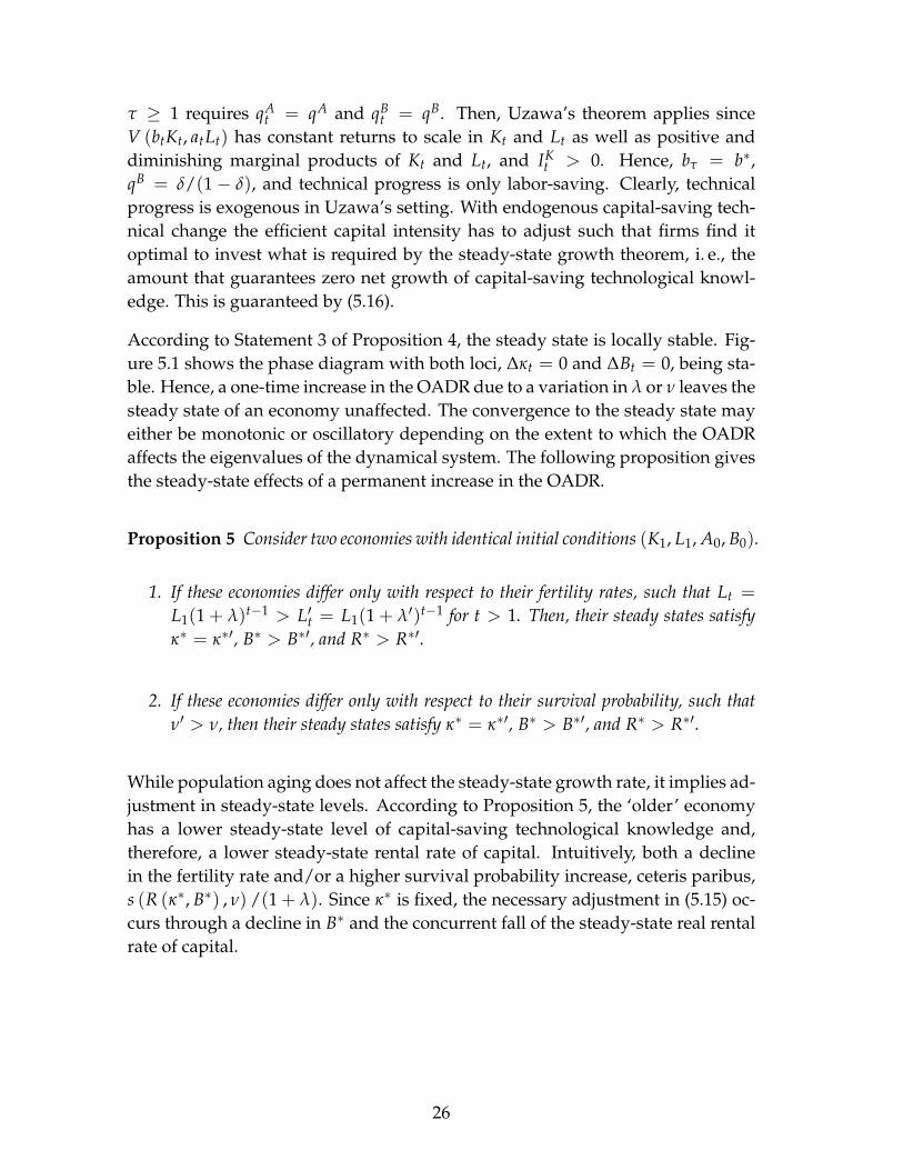
According to Statement 3 of Proposition 4, the steady state is locally stable. Fig-ure 5.1 shows the phase diagram with both loci, ∆κt = 0 and ∆Bt = 0, being sta-ble. Hence, a one-time increase in the OADR due to a variation in λ or ν leaves thesteady state of an economy unaffected. The convergence to the steady state mayeither be monotonic or oscillatory depending on the extent to which the OADRaffects the eigenvalues of the dynamical system. The following proposition givesthe steady-state effects of a permanent increase in the OADR.

Proposition 5 Consider two economies with identical initial conditions (K1, L1, A0, B0).

1. If these economies differ only with respect to their fertility rates, such that Lt =

L1(1 + λ)t−1 > L′t = L1(1 + λ′)t−1 for t > 1. Then, their steady states satisfyκ∗ = κ∗′, B∗ > B∗′, and R∗ > R∗′.

2. If these economies differ only with respect to their survival probability, such thatν′ > ν, then their steady states satisfy κ∗ = κ∗′, B∗ > B∗′, and R∗ > R∗′.

While population aging does not affect the steady-state growth rate, it implies ad-justment in steady-state levels. According to Proposition 5, the ‘older’ economyhas a lower steady-state level of capital-saving technological knowledge and,therefore, a lower steady-state rental rate of capital. Intuitively, both a declinein the fertility rate and/or a higher survival probability increase, ceteris paribus,s (R (κ∗, B∗) , ν) /(1 + λ). Since κ∗ is fixed, the necessary adjustment in (5.15) oc-curs through a decline in B∗ and the concurrent fall of the steady-state real rentalrate of capital.

26

6 Discussion and Extensions

6.1 The Role of Capital-Saving Technical Change

To further explore the role of capital-saving technical change, it proves useful toestablish and compare the effect of population aging in an economy without it. Toaccomplish this, recall that the dynamical system of Proposition 1 nests the caseof an economy with endogenous labor-saving technical change only. It obtainswhen, for all t, bt = Bt = 1 is fixed and qB

t (m) = 0. Then, given (K1, L1, A0, 1) > 0as initial conditions and (4.11), the dynamical system determines a unique equi-librium sequence {κt}∞

t=1 that satisfies

s (R (κt+1) , ν)

1 + λw (κt) = κt+1 (1− δ)

(1 +

(1 + ηA

)gA (κt+1)

),

with κ1 given by

κ1 =K1

A0 (1− δ) (1 + (1 + ηA) gA (κ1)) L1> 0.

Does this economy respond to population aging in the same way as the one withcapital-saving technical change? To see that the answer is no, consider the phasediagram of Figure 6.1. Suppose the economy starts in the steady state (κ∗, B∗)before it experiences a one-time and permanent decline in λ or increase in ν.This shock shifts the ∆κt = 0 and the ∆Bt = 0 loci downwards to intersect at(κ∗′, B∗′). The economy without capital-saving technical change converges to thenew steady state at κ∗A since the ∆κt = 0 locus is stable and Bt = B∗ remains con-stant. Intuitively, along the transition there is continuous capital deepening in-ducing more and more labor-saving technical change. As a consequence, popula-tion aging is associated with an increase in the steady-state growth rate.25 How-ever, if capital-saving technical change is possible, (κ∗A, B∗) cannot be a steadystate: to the right of κ∗, the growth rate of Bt is strictly negative. Following theinitial shock the economy lands on a trajectory with κt > κ∗ and Bt < B∗ and, asshown in Figure 6.1, may converge to the new steady state (κ∗, B∗′).

25These two forces are behind the steady-state analysis that appears, e. g., in Heer and Irmen(2009). A similar mechanism drives the results of population aging on the steady-state growthrate in Futagami and Nakajima (2001). The AK-model in Li, Zhang, and Zhang (2007) exhibits ajump that corresponds to a shift from (κ∗, B∗) to (κ∗A, B∗) without a transition period.

27

Figure 6.1: Comparative Statics and Dynamics of a One-Time and PermanentDecline (Increase) in the Growth Rate of the Labor Force (Survival Probability).The Case of a Stable Node.

6.2 Capital-Saving Investments with Contemporaneous Knowl-edge Spill-Overs

Thus far, the external contemporaneous knowledge spill-overs are confined tolabor-saving investments. Authors like Frankel (1962) or Romer (1986) advocatethe presence of such spill-overs in the context of capital investments. One way tocapture this is to replace bt(m) of (3.6) by

bt(m) = Bt−1 (1− δ)(

1 + qBt (m) + ηBeB

t

),

(6.1)

eBt ≡ 1

mt

∫ mt

0qB

t (m)dm,

where eBt is the external knowledge spill-over and ηB ∈ R+ measures its strength.

The incorporation of these knowledge spill-overs requires few modifications. Forinstance, the reasoning that led to Lemma 1 gives now rise to the map gB :R++ → R++, where qB

t = gB (κt, ηB) with gBηB(κt, ηB) < 0. Proposition 2 for

the short run as well as all qualitative findings for the long-run remain valid. Themost striking new aspect concerns the role of population aging for the evolution

28

of income. Due to the new external knowledge spill-over I have for the samereasons that explain Lemma 3

∂Vt

∂qBt

=ηBRtKt

1 + (1 + ηB) qBt> 0. (6.2)

The consequence is that the induced effects that appear in both lines of (5.6) arenow of opposite sign. Hence, EL

t and EKt can no longer be signed. However, the

signs for dVt+1/dKt+1 and dVt+1/dLt+1 as established in (5.14) remain valid.26 Asa result, the qualitative results of Proposition 3 remain true.

6.3 Changing Demographic Features

Three Generations Following, e. g., Bommier and Lee (2003), one may argue thata representation of economic life by three periods, childhood, adulthood, and oldage, is called for to study the implications of population aging. To incorporatethis consider three generations alive at each period t ≥ 1, i. e., νLt−1 retired old,Lt working adults, and Lt+1 children. At the beginning of period t, each work-ing adult gives birth to (1 + λt+1) offspring and maximizes his expected lifetimeutility (3.2) having the offspring consumption included in cy

t .27

However, for two reasons the relevance of this extension is rather limited in thepresent context. First, for the short-run effects the crucial link is between fertilityof adults at t and the supply of labor at t + 1. Adding a period of childhood doesnot affect this link. Therefore, the consequences of a decline in fertility stated inProposition 2 and Proposition 3 remain valid. To the extent that fewer childrenreduce total population, an increase in per-capita income becomes more likely iffertility declines in two successive periods, i. e., condition (5.10) will be easier tosatisfy for v′t+1 > vt+1. Second, the steady state is independent of the economy’sdemographic structure. Hence, in the long run, the amount of periods an individ-ual is supposed to live through does not affect the growth rate of the economy.

26To see this formally, denote ELt and EK

t of (5.6) by ELt(ηA, ηB) and EK

t(ηA, ηB), respec-

tively. Then, (6.2) implies ELt(ηA, ηB) > EL

t(ηA, 0

). Hence, wt + EL

t(ηA, ηB) > 0. Similarly,

EKt(ηA, ηB) > EK

t(0, ηB). Therefore, applying the reasoning set out in Footnote 21 to EK

t(0, ηB)

reveals that Rt + EKt(ηA, ηB) > 0.

27This setup has been studied by, e. g., Li, Zhang, and Zhang (2007). Here, the total depen-dency ratio may be a more appropriate indicator of economic dependency. It is equal to thesum of the old-age dependency ratio and the child dependency ratio, i. e., (νLt−1 + Lt+1) /Lt =

ν/ (1 + λt) + (1 + λt+1) .

29

Underestimation of Survival Rates Perfect foresight includes the assumptionthat young individuals correctly foresee their survival rates. This seems unre-alistic, especially in times where this rate considerably increases between gen-erations.28 One crude way to account for this is to allow for myopic foresightwhere the expected survival rate of cohort t is νt−1, i. e., the known survival rateof their parents. Then, an actual increase in the survival rate of cohort t has noeffects on their savings and the important effect of changes in ν on Kt+1/Lt+1 de-rived in (5.4) vanishes. As a consequence, the effects of an increase in ν statedin Proposition 2 are just postponed by one period. The same is true for Propo-sition 3: the savings channel is mute between t and t + 1 so that V′t+1 = Vt+1 in(5.11) and v′t+1 < vt+1 in (5.12). Underestimation of the survival rates leaves thesteady-state growth rate unaffected.

6.4 Endogenous Labor Supply

Individuals may want to increase their labor supply in anticipation of a higherwage. However, at the level of economic aggregates a higher individual laborsupply reduces, ceteris paribus, the capital-labor ratio. This weakens the incen-tive to increase labor productivity in accordance with Lemma 1 and Lemma 2 andreduces the wage. To address this tension assume that the individual labor sup-ply is an increasing function of the current wage in efficiency units. To be precise,denote τt ∈ [0, 1] the fraction of an individual’s time endowment that she suppliesto the labor market in t. Assume further that τt = τ(wt) where τ : R++ → [0, 1]with τ′(wt) > 0 > τ′′(wt). Then, with Lemma 1, I have τt = τ (w (κt)) and

ετκ(κt) ≡

d ln τt

d ln κt> 0.

Aggregate labor supply becomes τ (w (κt)) Lt. This affects Lemma 2 to the extendthat the response of κt to changes in Kt/Lt is weaker. In fact, adding the new termin the denominator of (4.5) reveals that the response of κt = κ (Bt−1Kt/At−1Lt) tochanges in the capital-labor ratio is now

εκ (κt) ≡d ln κt

d ln (Kt/Lt)=

11 + εA

κ (κt, ηA) + εBκ (κt) + ετ

κ (κt)∈ (0, 1). (6.3)

Intuitively, at the extensive margin, the scarcity of labor increases with Kt/Lt.However, at the intensive margin individuals supply more labor at the resulting

28See, e. g., Groneck, Ludwig, and Zimper (2011) for a discussion of behavioral biases in indi-vidual forecast errors of survival rates and their explanations.

30

higher wage. Hence, labor becomes more abundant. Nevertheless, the effectthrough the extensive margin remains dominant.

As a consequence, Proposition 1 remains valid. Moreover, the short-run effects ofaging have to include the fact that now a change in factor endowments not onlyinduces technical change as in (5.6) but also affects labor supply. Accordingly,(5.14) becomes

dVt+1

dKt+1= R2 + EK

t+1 + F2 at+1Lt+1τ′ (wt+1) wκ(κt+1))∂κt+1

∂Kt+1,

(6.4)dVt+1

dLt+1= w2 + EL

t+1 + F2 at+1Lt+1τ′ (wt+1) wκ(κt+1))∂κt+1

∂Lt+1,

where the argument of F2 is (bt+1Kt+1, at+1τt+1Lt+1). The new effect on laborsupply strengthens dVt+1/dKt+1 and weakens dVt+1/dLt+1. Incorporating thisin Proposition 2 reveals that the positive effect of a higher survival probability onaggregate income becomes more pronounced. Moreover, its effect on per-capitaincome is more likely to be positive. With an endogenous labor supply, the effectof a decline in fertility becomes more involved as long as εs

R 6= 0. In the specialcase where εs

R = 0 endogenous labor supply makes it more likely that incomeincreases in absolute and per-capita terms with population aging as individualswill also work longer hours. Clearly, this extension does not affect the qualitativeresults concerning the long run.

Alternatively, labor supply may depend positively on the expected survival prob-ability if people want to earn and save more expecting a longer period of retire-ment. To account for this let τt = τ(ν) where τ : R++ → [0, 1] with τ′(ν) > 0. Ac-counting for this in (4.5) reveals that Lemma 2 must be extended since κt = κ (·, ν)

with κν < 0. Hence, a higher survival probability reduces the equilibrium taskintensity since it increases the supply of labor. Then (5.2) becomes

s(

R(

κ(

BtKt+1AtLt+1

, ν)

, Bt

), ν)

1 + λwt =

Kt+1

Lt+1τ(ν). (6.5)

Moreover, as long as sR ≥ 0, it holds that ∂ (Kt+1/Lt+1) /∂ν > 0 so that thequalitative results of Proposition 2 remain valid.

Proposition 3 must be modified since now ν induces technical change that affectsaggregate income. To account for this use the same steps that lead to (5.6) andobtain

Eνt =

[∂Vt

∂qAt

gAκ

(κt, ηA

)+

∂Vt

∂qBt

gBκ (κt)

]∂κt

∂ν< 0, (6.6)

31

where the sign follows with Lemma 3. Intuitively, a higher life-expectancy meansa larger labor supply and, therefore, less induced labor-saving technical change.Hence, output falls. This effect will pop up in the modified statements of (5.11)and (5.12) and weaken the prospect that population aging fosters aggregate andper-capita income growth. Again, this extension leaves the qualitative results onsteady-state growth unaffected.

6.5 Endogenous Fertility

The question about the the repercussions between the evolution of the economyand its fertility rate is among the most challenging. A satisfactory discussionwould certainly require the incorporation of a fully endogenous fertility choice.However, this is beyond the scope of this paper.29 Nevertheless let me capture theidea and stipulate a functional relationship where the fertility rate of generationt depends in a negative way on its survival probability, i. e., λt = λ(ν), where λ :[0, 1] → (−1, ∞) with λ′(ν) < 0. This specification is consistent with the recentexperience of the industrialized world where fertility declines as life expectancyincreases. This relationship may be driven, e. g., by advances in the life and themedical sciences.

With this specification the old-age dependency ratio is ν/ (1 + λ(ν)), and the ef-fect of increasing ν becomes more pronounced as the current young reduce theirfertility in anticipation of a higher survival probability. The most important mod-ification of this feature concerns the clear-cut prediction that a rise in the survivalprobability increases aggregate income made in Proposition 3. Going through thesteps that lead to (5.11), one now finds

V′t+1 R Vt+1 if

[(Rt+1 + EK

t+1

)( Kt+1

1 + λ(ν)

−ε

1− ε

)+(

wt+1 + ELt+1

)]λ′(ν)(ν′ − ν)

(6.7)

+(

Rt+1 + EKt+1

)( sν (Rt+1, ν)wt

1− ε

)(ν′ − ν) R 0,

The first line of (6.7) states the new effect on income that a rise in the survivalprobability induces through a decline in fertility. From the discussion of (5.9)

29See, e. g., Becker, Murphy, and Tamura (1990) or Galor (2011) for a discussion of the fertility-growth nexus.

32

this effect is negative if sR ≥. Accordingly, the positive effect of an increase inlife-expectancy on economic growth through an increase in savings is weakened.Clearly, the steady-state growth rate will not depend on whether fertility is en-dogenous or not.

7 Concluding Remarks

This paper studies the role of population aging for economic growth. It claimsthat demographic change affects the investment behavior of firms with implica-tions for technical progress and economic growth. A central result of the analysisis that the type of technical progress is crucial for the link between populationaging and economic growth. To make this point, this paper extends the existingliterature and allows for two types of endogenous technical progress, i. e., capital-and labor-saving technical change.

Capital-saving technical change is found to imply that the steady-state growthrate is independent of the economy’s age structure. Hence, in the long run, eco-nomic growth is independent of demographic features. However, populationaging affects economic growth along the transition since it accentuates the rela-tive scarcity of labor with respect to capital. This leads to more labor- and lesscapital-saving technical change. Due to external contemporaneous knowledgespill-overs, this induced change in the direction of technical change is found tohave first-order effects on the evolution income.

The present analysis suggests several routes for future research. They include thequestion about how population aging affects economic growth if the age structureof the labor force matters for the direction of technical change. Case studies likeNishimura, Minetaki, Shirai, and Kurokawa (2002) for Japan, Prskawetz, Kogel,Sanderson, and Scherbov (2007) for India, or the panel study of Feyrer (2007)suggest a role of population aging for economic growth beyond its effect on thescarcity of the entire labor force relative to capital.

Second, one may want to inquire into the scope for design of growth policies tomeet the economic challenges of population aging. This will require an analysisof the welfare properties of the equilibrium. Due to the presence of contempo-raneous and inter-temporal external effects the equilibrium will in general notbe efficient. This leaves room for fiscal policy measures to improve the norma-tive properties of the competitive equilibrium. However, the main insight of thispaper suggests that the effects and the desirability of any growth policy will cru-cially depend on whether technical change is capital-saving in addition to beinglabor-saving. I leave these questions for future research.

33

A Proofs

A.1 Proof of Lemma 1

Consider (3.9) - (3.12) at qAt (n) = qA

t = eAt and qB

t (m) = qBt . Upon substitution of (3.9) in (3.11)

and (3.10) in (3.12) I obtain

f (κt)− κt f ′ (κt) =(

1 +(

1 + ηA)

qAt

)i′(

qAt

)+ i(

qAt

),

(A.1)

f ′ (κt) =(

1 + qBt

)i′(

qBt

)+ i(

qBt

).

Denote RHS(q, η) the right-hand side of both conditions with the understanding that η = 0 inthe second one. In view of the properties of the function i given in (3.7), RHS(q, η) is a mappingRHS : R2

+ → R+ with limq→0 RHS(q, η) = 0, RHSq(q, η) > 0 for q > 0, limq→0 RHSq(q, η) =

i′′(q) ≥ 0, and limq→∞ RHS(q, η) = ∞. Moreover, the properties of the function f (κt) imply thatthe left-hand side of both conditions is strictly positive for κt > 0. Hence, for each κt > 0 thereis a unique qj

t > 0, j = A, B, that satisfies the respective condition stated in (A.1). I denote thesemaps by qA

t = gA (κt, ηA) and qBt = gB (κt), respectively.

An application of the implicit function theorem to (A.1) gives dqAt /dκt ≡ gA

κ

(κt, ηA) > 0, dqA

t /dηA ≡gA

ηA

(κt, ηA) < 0, and dqB

t /dκt ≡ gBκ (κt) < 0. The respective signs follow from the properties of

the functions f and i.

With qAt = gA (κt, ηA) and qB

t = gB (κt), I may express wt and Rt using the respective first-ordercondition of (3.9) and (3.10). Then,

wt = At−1 (1− δ)(

1 +(

1 + ηA)

gA(

κt, ηA))2

i′(

gA(

κt, ηA))≡ w (κt, At−1) ,

(A.2)

Rt = Bt−1 (1− δ)(

1 + gB (κt))2

i′(

gB (κt))≡ R (κt, Bt−1) .

The properties stated in (3.14) are immediate. For further reference, notice that the sign of thepartial derivatives wκ (κt, At−1) and Rκ (κt, Bt−1) carry over to the respective factor prices in ef-ficiency units, i. e., to w (κt) ≡ w (κt, At−1) /at =

(1 +

(1 + ηA) gA (κt)

)i′(

gA (κt))

and R (κt) ≡R (κt, Bt−1) /bt =

(1 + gB (κt)

)i′(

gB (κt))

. �

A.2 Proof of Lemma 2

Equation (4.5) is a fixed-point problem with a unique solution κ(

Bt−1Kt/At−1Lt, ηA) > 0. To seethis, write the right-hand side of (4.5) as RHS

(κt, Bt−1Kt/At−1Lt, ηA). Given the properties of

gA (κt, ηA) and gB (κt) as stated in (3.13) and Bt−1Kt/At−1Lt > 0, RHS(κt, Bt−1Kt/At−1Lt, ηA)

is a function which is continuous, strictly decreasing, and strictly positive for all κt > 0. Hence,limκt→0 RHS (κt, ·) > 0. Accordingly, there is a unique κ > 0 such that κ = RHS (κ, ·). Implicitdifferentiation of (4.5) delivers (4.7). �

34

A.3 Proof of Proposition 1

Given (Kt, Lt, At−1, Bt−1), it is straightforward to establish that the variables κt and Bt are indeedstate variables of the economy at t. To prove the existence of a unique equilibrium sequence{κt, Bt}∞

t=1 let me first derive equation (4.9). To do so solve (4.5) for Kt+1 and substitute the re-sulting expression into (4.8). Using st = s (R (κt+1, Bt) , ν)w (κt) and w (κt) ≡ w(κt)/at gives (4.9)after some straightforward manipulations. The difference equation (4.10) is from (3.16) where qB

tis replaced by gB (κt) in accordance with Lemma 1. In the first period, κ1 is pinned down by (4.5)for given initial values (K1, L1, A0, B0, ) > 0. From Lemma 2, there is a unique solution κ1 > 0.

To prove the uniqueness of the sequence {κt, Bt}∞t=1 it is useful to introduce

Ψ (κt, Bt−1) ≡1 +

(1 + ηA) gA (κt, ηA)

1 + gB (κt)

κt(1 + λ)

s (R (κt, Bt−1) , ν). (A.3)

Then, (4.9) may be written as

Bt w (κt) = Ψ (κt+1, Bt) . (A.4)

From (A.2) the left-hand side of (A.4) is strictly positive for any (κt, Bt) ∈ R2++. Hence, there is a

unique value κt+1 > 0 that satisfies (A.4) if Ψ (κt+1, Bt) is strictly positive, continuous, monotonein κt+1, and may take on all values in R2

++ as κt+1 varies.

To see that the latter properties are indeed fulfilled, observe that Ψ (κ, Bt) > 0 for κ > 0. Thisfollows from the definition of Ψ, Lemma 1, and s (Rt+1, ν) ∈ (0, 1). Let me simplify the notationfor the remainder of this proof and write s (R(κ)) for s (R(κ, Bt), ν). Then, one readily verifies thatΨκ (κ, Bt) > 0 for κ > 0 is assured if(

sR (R(κ))R(κ)

s (R(κ))

)(Rκ(κ)

κ

R(κ)

)< 1 + εA

κ

(κ, ηA

)+ εB

κ (κ). (A.5)

Observe with (3.3) and (3.14) that the left-hand side of (A.5) is εsR(κ) · εR

κ (κ). From (4.5), the right-hand side is equal to 1/εκ . Hence, (A.5) coincides with (4.11).

Next , I show that limκ→0 Ψ (κ, Bt) = 0 and limκ→∞ Ψ (κ, Bt) = ∞. To make the argument, onehas to consider both factors on the right-hand side of (A.3).

First, since gA (κ, ηA) is increasing in κ on R++ and bounded from below by zero, limκ→0 gA (κ, ηA)is finite and limκ→∞ gA (κ, ηA) is finite or infinite. Since gB (κ) is decreasing on R++ and boundedfrom below by zero, limκ→0 gB (κ) is either finite or infinite and limκ→∞ gB (κ) is finite. As a con-sequence, limκ→0

(1 +

(1 + ηA) gA (κ, ηA)) /

(1 + gB (κ)

)is finite, and

limκ→∞(1 +

(1 + ηA) gA (κ, ηA)) /

(1 + gB (κ)

)is either finite or infinite.

Second, I have to know the limits limκ→0 κ/s (R(κ)) and limκ→∞ κ/s (R(κ)). As to the limit κ → 0,the following cases must be considered. First, if limκ→0 R(κ) = R(0) is finite, then s (R(0)) ∈ (0, 1)and limκ→0 κ/s (R(κ)) = 0. Second, if limκ→0 R(κ) = R(0) is infinite, then limκ→∞ s (R(κ)) =

s (R(0)) ≥ 0. If s (R(0)) > 0, then it is immediate that limκ→0 κ/s (R(κ)) = 0. If s (R(0)) = 0,then savings goes to zero as the rental rate of capital approaches infinity. However, even in thiscase it holds that limκ→0 κ/s (R(κ)) = 0. To see this, consider the Euler equation of cohort t,u′(co

t+1) = u′(cyt )/R(κ). By assumption, limκ→0 R(κ) = ∞ and limκ→0 s (R(κ)) = 0. Therefore,

limκ→0

u′(cyt )

R(κ)= lim

κ→0

u′((1− s (R(κ)))wt)

R(κ)=

u′(wt)

limκ→0 R(κ)= 0.

35

Hence, from the Euler condition limκ→0 u′(co

t+1)= 0. Since u satisfies the Inada condition, I find

with the budget constraint of an old individual at t + 1

limκ→0

cot+1 =

wt

νlimκ→0

[R(κ) s (R(κ))] = ∞. (A.6)

Next, observe that f (κ) > κ f ′(κ) > 0 since F2 > 0 for κ > 0. Then, using (3.12) and qB = gB(κ), Imay express κR(κ) as

κR(κ) = Bt (1− δ)(

1 + gB (κ)) [

κ f ′(κ)− κi(

gB (κ))]

(A.7)

< Bt (1− δ)(

1 + gB (κ)) [

f (κ)− κi(

gB (κ))]≡ R(κ).

Then, for κ < 1, κR(κ) < R(1). Therefore,

s (R(κ))κ

=R(κ)s (R(κ))

κR(κ)>

R(κ)s (R(κ))R(1)

. (A.8)

In light of (A.6) , limκ→0 s (R(κ)) /κ = ∞, and limκ→0 κ/s (R(κ)) = 0 as desired. Therefore,limκ→0 Ψ(κ, Bt) = 0.

Finally, note that limκ→∞ κ/s (R(κ)) = ∞ since limκ→∞ s (R(κ)) ∈ [0, 1]. Hence, limκ→∞ Ψ(κ, Bt) =

∞.

Hence, the right-hand side of (A.4) is increasing on R++ approaching zero as κ → 0 and infinityas κ → ∞. Accordingly, there is a unique κ that satisfies (4.9) given (κt, Bt) ∈ R2

++. With thisvalue at hand, (4.10) delivers a unique Bt+1 > 0. �

A.4 Proof of Proposition 2

This proposition follows immediately from (5.3), (5.4), Lemma 1, and Lemma 2. �

A.5 Proof of Lemma 3

Consider (5.5). With at and bt from (3.16) and (3.9) I find,

∂Vt

∂qAt

= At−1(1− δ)(

1 + ηA)

Lt

[F2 (btKt, atLt)− i

(qA

t

)−(

1 +(

1 + ηA)

qAt

)i′(

qAt

)]

+ ηA At−1(1− δ)Lt

(1 +

(1 + ηA

)qA

t

)i′(

qAt

)=

ηAwtLt

1 + (1 + ηA) qAt

> 0,

(A.9)∂Vt

∂qBt

= Bt−1(1− δ)Kt

[F1 (btKt, atLt)− i

(qB

t

)−(

1 + qBt

)i′(

qBt

)]= 0.

In equilibrium the expressions in brackets vanish in accordance with (A.1). Hence, (5.7) is shown.The results stated in (5.8) are immediate from Lemma 1, Lemma 2, and (5.6). �

36

A.6 Proof of Proposition 3

Claim 1 Consider λ′ < λ sufficiently close. Simplifying the notation, I denote Vt+1 ≡ V (Kt+1, Lt+1)

the equilibrium income under λ. Here, it is understood that

qAt+1 = gA

(κ (BtKt+1/AtLt+1) , ηA

)and qB

t+1 = gB (κ (BtKt+1/AtLt+1)) (A.10)

in accordance with Lemma 1 and Lemma 2. Similarly, under λ′ the equilibrium income is V′t+1 ≡V(K′t+1, L′t+1

), where qA′

t+1 and qB′t+1 differ from (A.10) as they now depend on K′t+1/L′t+1.

Step 1: For (Kt+1, Lt+1) and(K′t+1, L′t+1

)sufficiently close, (5.13) states the first-order Taylor ap-

proximation of V′t+1 at Vt+1 (Kt+1, Lt+1). As explained in the main text, the total effect of a smallchange of Kt+1 and Lt+1 on Vt+1 may be written as in (5.14).

Step 2: To quantify the difference K′t+1 − Kt+1, consider the Taylor approximation K′t+1 ≈ Kt+1 +

∂Kt+1/∂λ(λ′ − λ) at λ. The derivative involved is obtained from

s(

R(

κ

(BtKt+1

AtLt(1 + λ)

), Bt

), ν

)wtLt = Kt+1, (A.11)

which restates (4.8) using Lemma 1, Lemma 2, and Lt+1 = Lt(1 + λ) to uncover the dependencyof Kt+1 on λ. Implicit differentiation delivers

∂Kt+1

∂λ=

Kt+1

1 + λ

−ε

1− εR 0 ⇔ εs

R R 0, (A.12)

where all elasticities are evaluated at κt+1. Hence,

∂Kt+1

∂λR 0 ⇔ εs

R R 0 and K′t+1 R Kt+1 ⇔ εsR Q 0. (A.13)

Finally, noting that L′t+1 − Lt+1 = Lt(λ′ − λ) I have

dVt+1 ≡ V′t+1 −Vt+1 ≈dVt+1

dKt+1

∂Kt+1

∂λ

(λ′ − λ

)+

dVt+1

dLt+1Lt(λ′ − λ

). (A.14)

Then, straightforward manipulations deliver (5.9).

To prove (5.10) consider dvt+1 ≡ v′t+1 − vt+1, where vt+1 = Vt+1/ (Lt (ν + 1 + λ)) and v′t+1 =

V′t+1/ (Lt (ν + 1 + λ′)). With dVt+1 of (A.14) I have

dvt+1 ≈ dVt+1/ (Lt (ν + 1 + λ))−Vt+1(λ′ − λ

)/(

Lt (ν + 1 + λ)2)

.

Hence,

dvt+1 Q 0 ⇔ dVt+1 − vt+1Lt(λ′ − λ) Q 0. (A.15)

Straightforward manipulations using the results derived above reveal that (A.15) coincides with(5.10). Hence, Claim 1 of Proposition 3 is proven.

Claim 2 Consider ν′ > ν sufficiently close.

Step 1: The first-order Taylor approximation at (Kt+1, Lt+1) is now

dVt+1 ≡ V′t+1 −Vt+1 ≈ dVt+1

dKt+1(K′t+1 − Kt+1), (A.16)

37

taking into account that L′t+1 = Lt+1.

Step 2: To quantify the difference K′t+1 − Kt+1, consider the Taylor approximation K′t+1 − Kt+1 ≈∂Kt+1/∂ν(ν′ − ν) at ν. The derivative involved may be directly derived from (5.4) noting thatLt+1∂ (Kt+1/Lt+1) /∂ν = ∂Kt+1/∂ν. Hence,

∂Kt+1

∂ν=

sν (Rt+1, ν)wtLt

1− ε> 0, (A.17)

where the elasticities are evaluated at κt+1. The sign follows from sν > 0 in conjunction with(4.11). Hence,

K′t+1 R Kt+1 ⇔ ν′ R ν. (A.18)

To prove (5.12) consider again dvt+1 ≡ v′t+1 − vt+1. The result follows from the same steps thatled to (A.15) with ν′ − ν replacing λ′ − λ. Then, straightforward manipulations using the resultsderived above deliver inequality (5.12). This completes the proof of Proposition 3. �

A.7 Proof of Proposition 4

1. “⇒”: If condition (5.17) holds, then, at qBt = δ/(1− δ), (3.10) and (3.12) deliver a unique

κ∗ ∈ (0, ∞) since f ′(κ) < 0 on R++. To see that there also exists a unique B∗ ∈ R2++,

rewrite (5.15) as B∗s (R(κ∗, B∗), ν) = const. > 0. Since sR(·) ≥ 0, the left-hand side isstrictly increasing in B∗ taking on values form zero to infinity as B∗ varies on this interval.Hence, there is a unique value B∗ > 0 that satisfies (5.15).

“⇐”: If i′ (δ/(1− δ)) /(1− δ) + i (δ/(1− δ)) ≥ limκ→0 f ′(κ), then (3.12) delivers mt = 0,hence κt = 0. If limκ→∞ f ′(κ) ≥ i′ (δ/(1− δ)) /(1− δ) + i (δ/(1− δ)) then (3.12) deliversmt = ∞, hence κt = ∞.

2. Since (5.16) determines κ∗, I obtain g∗ from Lemma 1 and (3.16). The stated findings aboutthe steady-state growth factors of at, wt, cy

t , cot , and st are immediate from at = At, (A.2),

(3.3), and the budget constraints. Steady-state growth of Kt follows from (4.8). All othergrowth factors under b) result from (3.4) in conjunction with (E4), and (4.3). Finally, (3.16)gives bt = B∗, (A.2) delivers R∗ = B∗i′(δ/(1− δ))/(1− δ), and σt evaluated at the steadystate gives σ∗.

3. From the proof of Proposition 1, I know that (4.11) implies Ψκ (κt+1, Bt) > 0. Similarly, onereadily verifies that ΨB (κt+1, Bt) ≤ 0 if sR(·) ≥ 0. It is then straightforward to see that (4.9)defines a continuously differentiable function φκ : R2

++ → R++, i. e., κt+1 = φκ(κt, Bt).Consider (4.10) for t + 1 and substitute κt+1 = φκ (κt, Bt). This gives

Bt+1 = Bt(1− δ)(

1 + gB (κt+1))= Bt(1− δ)

(1 + gB (φκ (κt, Bt))

)≡ φB (κt, Bt) , (A.19)

which is also a continuously differentiable function φB : R2++ → R++. Hence, with (κ1, B1)

given by (4.10) and (4.12), the dynamical system can be stated as

(κt+1, Bt+1) = φ (κt, Bt) ≡(

φκ(κt, Bt), φB(κt, Bt))

, t = 1, 2, ..., ∞. (A.20)

The steady state is a fixed point of (A.20). To study the local behavior of the system aroundthe steady state, I need the eigenvalues of the Jacobian Dφ(κ∗, B∗). I study each of its fourelements in turn.

38

(a) First, consider φκ(κt, Bt). Implicit differentiation of (A.4) and evaluation at the steadystate gives

φκκ(κ∗, B∗) =

B∗ wκ (κ∗)

Ψκ (κ∗, B∗)> 0, (A.21)

where use is made of (A.2) and Ψκ (κ∗, B∗) > 0. Assuming that the set ∆κt = 0 is sta-ble in the vicinity of the steady state is equivalent to the assumption that φκ

κ(κ∗, B∗) ∈

(0, 1). Similarly, I obtain

φκB(κ∗, B∗) =

Ψ (κ∗, B∗)− B∗ΨB (κ∗, B∗)B∗ Ψκ (κ∗, B∗)

> 0, (A.22)

since ΨB (κ∗, B∗) ≤ 0. Finally, note that (A.21) and (A.22) imply that the slope of theset ∆κt = 0 is positive, i. e., dBt/dκt|∆κt=0 = (1− φκ

κ(κ∗, B∗))/φκ

B(κ∗, B∗) > 0.

(b) Second, consider φB (κt, Bt). From (A.19) I obtain

φBκ (κ∗, B∗) = B∗gB

κ (κ∗) φκκ (κ

∗, B∗) < 0 (A.23)

and

φBB (κ∗, B∗) = 1 + B∗gB

κ (κ∗) φκB (κ∗, B∗) < 1. (A.24)

Using (A.22) and the definition of Ψ given in (A.3), I find φBB (κ∗, B∗) ∈ (0, 1) if

εsκ(κ∗) < 1 + εA

κ (κ∗). The latter holds since εs

κ(κ∗) ≤ 0. Hence, the set ∆Bt = 0 is

stable in the vicinity of the steady state with monotonic convergence.Finally, note that (A.23) and (A.24) imply that the slope of the set ∆Bt = 0 is negative,i. e., dBt/dκt|∆Bt=0 = φB

κ (κ∗, B∗)/(1− φB

B(κ∗, B∗)) < 0.

Using (A.21) - (A.24), the required Jacobian may be written as

D φ(κ∗, B∗) =

φκκ(κ∗, B∗) φκ

B(κ∗, B∗)

B∗gBκ (κ∗) φκ

κ(κ∗, B∗) 1 + B∗ gB

κ (κ∗) φκB(κ∗, B∗)

.

Its eigenvalues, µ1, µ2, are given by

µ1,2 =φκ

κ + φBB

2±

√√√√(φκκ + φB

B2

)2

− φκκ .

Both eigenvalues are real if(φκ

κ + φBB)2 ≥ 4φκ

κ . Since 2 > φκκ + φB

B > 0, I have 1 > µ1 ≥µ2 > 0. Hence, the steady state is either a stable node if the weak inequality is strict or afocus if not. If

(φκ

κ + φBB)2

< 4φκκ , then Dφ has two distinct complex eigenvalues, and the

steady state is a spiral sink since det (Dφ) = φκκ < 1 (see, e. g., Galor (2007), Proposition

3.8). The stability of the sets ∆κt = 0 and ∆Bt = 0 imply a clockwise orientation of thespiral sink. �

A.8 Proof of Proposition 5

The steady-state efficient capital intensity is given by (5.16). Since gB (κ) is independent of λ andν, I have κ∗ = κ∗′. Moreover, since sν (R(κ∗, B∗), ν) > 0, sR (R(κ∗, B∗), ν) ≥ 0, and RB(κ

∗, B∗) > 0,(5.15) also delivers λ > λ′ ⇒ B∗ > B∗′ and ν′ > ν⇒ B∗′ < B∗. �

39

ReferencesACEMOGLU, D. (2003): “Labor- and Capital-Augmenting Technical Change,” Journal of European

Economic Association, 1(1), 1–37.

(2007): “Equilibrium Bias of Technology,” Econometrica, 75(5), 1371–1410.

(2010): “When Does Labor Scarcity Encourage Innovation?,” Journal of Political Economy,118(6), 1037–1078.

ACEMOGLU, D., AND S. JOHNSON (2007): “Disease and Development: The Effect of Life Ex-pectancy on Economic Growth,” Journal of Political Economy, 115(6), 925–985.

ALLAIS, M. (1947): Economie et Interet. Imprimerie National, Paris.

ASHRAF, Q. H., A. LESTER, AND D. N. WEIL (2009): “When Does Improving Health RaiseGDP?,” in NBER Macroeconomics Annual 2008, Volume 23, NBER Chapters, pp. 157–204. Na-tional Bureau of Economic Research, Inc.

BECKER, G. S., K. M. MURPHY, AND R. TAMURA (1990): “Human Capital, Fertility, and Eco-nomic Growth,” Journal of Political Economy, 98(5), S12–S37.

BLANCHARD, O. J. (1985): “Debt, Deficits, and Finite Horizons,” Journal of Political Economy, 93,223–247.

BLOOM, D. E., D. CANNING, AND G. FINK (2008): Population Aging and Economic Growth. TheInternational Bank for Reconstruction and Development / The World Bank - Commission onGrowth and Development, Washington, DC.

BLOOM, D. E., D. CANNING, AND B. GRAHAM (2003): “Longevity and Life-Cycle Savings,”Scandinavian Journal of Economics, 105(3), 319–338.

BLOOM, D. E., D. CANNING, AND J. SEVILLA (2003): The Demographic Dividend - New Perspectiveson the Economic Consequences of Population Change. Rand Cooperation, Santa Monica, CA.

(2004): “The Effect of Health on Economic Growth: A Production Function Approach,”World Development, 32(1), 1–13.

BOMMIER, A., AND R. D. LEE (2003): “Overlapping Generations Models with Realistic Demog-raphy,” Journal of Population Economics, 16(1), 135–160.

BOUCEKKINE, R., D. DE LA CROIX, AND O. LICANDRO (2002): “Vintage Human Capital, Demo-graphic Trends, and Endogenous Growth,” Journal of Economic Theory, 104, 340–375.

CERVELLATI, M., AND U. SUNDE (2011): “Life Expectancy and Economic Growth: the Role ofthe Demographic Transition,” Journal of Economic Growth, 16(2), 99–133.

CHAMPERNOWNE, D. G. (1961): “A Dynamic Growth Model Involving a Production Function,”in The Theory of Capital - Proceedings of a Conference Held by the International Economic Association,ed. by F. A. Lutz, and D. C. Hague, pp. 223–244. MacMillian (Reprinted 1963), London.

DE LA CROIX, D., AND O. LICANDRO (1999): “Life Expectancy and Endogenous Growth,” Eco-nomics Letters, 65, 255–263.

40

DE LA CROIX, D., AND P. MICHEL (2002): A Theory of Economic Growth – Dynamics and Policy inOverlapping Generations. Cambridge University Press, Cambridge, UK.

DIAMOND, P. A. (1965): “National Debt in a Neoclassical Growth Model,” American EconomicReview, 55(5), 1126–1150.

DRANDAKIS, E. M., AND E. S. PHELPS (1966): “A Model of Induced Invention, Growth, andDistribution,” The Economic Journal, 76, 823–840.

EUROPEAN COMMISSION - ECONOMIC AND FINANCIAL AFFAIRS - AMECO (2012): “UpdateMay 2012,” European Commission,http://ec.europa.eu/economy finance/ameco/user/serie/SelectSerie.cfm (accessed on August, 7, 2012).

FEYRER, J. (2007): “Demographics and Productivity,” The Review of Economics and Statistics, 89(1),100–109.

FRANKEL, M. (1962): “The Production Function in Allocation and Growth: A Synthesis,” Ameri-can Economic Review, 52(5), 995–1022.

FUTAGAMI, K., T. IWAISAKO, AND T. NAKAJIMA (2002): “Technological Innovation, Productiv-ity, and Economic Growth in Aging Societies,” in Economic Policy for Aging Societies, ed. byH. Siebert, pp. 163–173. Springer, Heidelberg.

FUTAGAMI, K., AND T. NAKAJIMA (2001): “Population Aging and Economic Growth,” Journal ofMacroeconomics, 23, 31–44.

GALOR, O. (2007): Discrete Dynamical Systems. Springer Verlag, Berlin – Heidelberg.

(2011): Unified Growth Theory. Princeton University Press, Princeton, NJ.

GRONECK, M., A. LUDWIG, AND A. ZIMPER (2011): “A Life-Cycle Consumption Model withAmbiguous Survival Beliefs,” Netspar Discussion Papers 03/2011-044.

HEER, B., AND A. IRMEN (2009): “Population, Pensions, and Endogenous Economic Growth,”Center for Economic Policy Research (CEPR), London, Discussion Paper, No. 7172.

HELLWIG, M., AND A. IRMEN (2001): “Endogenous Technical Change in a Competitive Econ-omy,” Journal of Economic Theory, 101, 1–39.

HICKS, J. R. (1932): The Theory of Wages. Macmillan, London, 1st edn.

IRMEN, A. (2005): “Extensive and Intensive Growth in a Neoclassical Framework,” Journal ofEconomic Dynamics and Control, 29(8), 1427–1448.

(2012a): “Endogenous Task-Based Technical Change - Factor Scarcity and Factor Prices,”mimeo, CREA, University of Luxembourg.

(2012b): “Innovation Investments and the Steady-State Growth Theorem,” mimeo, CREA,University of Luxembourg.

JONES, C. I. (2005): “The Shape of Production Functions and the Direction of Technical Change,”The Quarterly Journal of Economics, 120(2), 517–549.

41

KALDOR, N. (1961): “Capital Accumulation and Economic Growth,” in The Theory of Capital, ed.by F. A. Lutz, and D. C. Hague, pp. 177–222. Macmillan & Co. LTD., New York: St. Martin’sPress.

KLUMP, R., P. MCADAM, AND A. WILLMAN (2007): “Factor Substitution and Factor Augment-ing Technical Progress in the US: A Normalized Supply-Side System Approach,” Review ofEconomics and Statistics, 89(1), 183–192.

LI, H., J. ZHANG, AND J. ZHANG (2007): “Effects of Longevity and Dependency Rates on Savingand Growth: Evidence from a Panel of Cross Countries,” Journal of Development Economics, (84),138–154.

LORENTZEN, P., J. MCMILLAN, AND R. WACZIARG (2008): “Death and development,” Journal ofEconomic Growth, 13(2), 81–124.

LUCAS, R. E. (1988): “On the Mecanics of Economic Development,” Journal of Monetary Economics,22(5), 3–42.

MERKEL, A. (2009): “Wachstum. Bildung. Zusammenhalt. Deutschland zu neuer Starke fuhren -government declaration of chancellor Merkel in the German Federal Parliament 2009,” Presse-und Informationsamt der Bundesregierung.

MICHEL, P., AND D. DE LA CROIX (2000): “Myopic and Perfect Foresight in the OLG Model,”Economics Letters, 67, 53–61.

NISHIMURA, K. G., K. MINETAKI, M. SHIRAI, AND F. KUROKAWA (2002): “Effects of InformationTechnology and Aging Work Force on Labor Demand and Technological Progress in JapaneseIndustries: 1980-1998,” CIRJE F-Series CIRJE-F-145, CIRJE, Faculty of Economics, University ofTokyo.

PRETTNER, K. (2011): “Population Aging and Endogenous economic Growth,” Harvard Univer-sity, Program on the Global Demography of Aging, Working Paper No. 72.

PRETTNER, K., AND A. PRSKAWETZ (2010): “Demographic Change in Models of EndogenousEconomic Growth. A Survey,” Central European Journal of Operations Research, 12(4), 593–608.

PRSKAWETZ, A., T. KOGEL, W. SANDERSON, AND S. SCHERBOV (2007): “The Effects of AgeStructure on Economic Growth: An Application of Probabilistic Forecasting to India,” Interna-tional Journal of Forecasting, 23(4), 587–602.

ROMER, P. M. (1986): “Increasing Returns and Long-Run Growth,” Journal of Political Economy,94, 1002–1037.

SAMUELSON, P. A. (1958): “An Exact Consumption-Loan Model of Interest with or without theSocial Contrivance of Money,” Journal of Political Economy, 66, 467–482.

SOLOW, R. M. (1956): “A Contribution to the Theory of Economic Growth,” Quarterly Journal ofEconomics, 70(1), 65–94.

SWAN, T. W. (1956): “Economic Growth and Capital Accumulation,” Economic Record, 32, 334–361.

42

THE WORLD BANK (2012): “World Development Indicators,” The World Bank,http://data.worldbank.org/indicator/SP.POP.DPND.OL (accessed on August, 7, 2012).

TIROLE, J. (1985): “Asset Bubbles and Overlapping Generations,” Econometrica, 53(6), 1499–1528.

UNITED NATIONS (2011): “World Population Prospects: The 2010 Revision,” United Nations, NewYork, http://esa.un.org/unpd/wpp/Excel-Data/population.htm (accessed on July 4, 2011).

UZAWA, H. (1961): “Neutral Inventions and the Stability of Growth Equilibrium,” Review of Eco-nomic Studies, 28(2), 117–124.

YAARI, M. (1965): “Uncertain Lifetime, Life Insurance and the Theory of the Consumer,” Reviewof Economic Studies, 32(2), 137–150.

ZEIRA, J. (1998): “Workers, Machines, And Economic Growth,” Quarterly Journal of Economics,113(4), 1091–1117.

ZHANG, J., J. ZHANG, AND R. LEE (2001): “Mortality Decline and Long-Run Economic Growth,”Journal of Public Economics, 80, 485–507.

43