capital account opening and wage inequality · capital account opening and wage inequality ......

Capital Account Opening and Wage Inequality ∗

Mauricio Larrain†

Columbia University

This version: October 2014

ForthcomingReview of Financial Studies

Abstract

Opening the capital account allows financially-constrained firms to raise cap-ital from abroad. Since capital and skilled labor are relative complements, thisincreases the relative demand for skilled labor versus unskilled labor, leadingto higher wage inequality. Using aggregate data and exploiting variation in thetiming of capital account openings across 20 mainly European countries, I findthat opening the capital account increases aggregate wage inequality. In orderto identify the mechanism, I use sectoral data and exploit variation in externalfinancial dependence and capital-skill complementarity across industries. I findthat capital account opening increases sectoral wage inequality, particularly inindustries with both high financial needs and strong complementarity.

∗I am indebted to Atif Mian, for his invaluable guidance and encouragement. I also thank GeertBekaert, Murillo Campello, David Card, Todd Gormley (discussant), Yuriy Gorodnichenko, AntonKorinek (discussant), Ross Levine, Ulrike Malmendier, Ted Miguel, Elias Papaioannou (discussant),Emmanuel Saez, and Daniel Wolfenzon for their helpful comments. This paper also benefited from thecomments of seminar participants at the Boston Fed, Brown University, Columbia Business School,Federal Reserve Board, Princeton University, UBC Sauder, Chicago Booth, UC Berkeley, Universityof Notre Dame, IMF, Pac-Dev, Midwest Macro Meetings, WFA conference, LBS Summer Symposium,and several institutions in Chile. I also thank Andrew Karolyi (the Editor) and two anonymous refereesfor their valuable feedback. I am grateful for funding from the Kauffman Foundation and the Centerfor Equitable Growth at UC Berkeley. This paper was previously circulated under the title “DoesFinancial Liberalization Contribute to Wage Inequality? The Role of Capital-Skill Complementarity.”†Columbia Business School. Mailing address: 3022 Broadway, Uris Hall 813. New York, NY,

10027. Phone number: 212-851-0175. E-mail address: [email protected].

1

1 Introduction

In the last four decades, many developed and developing countries have opened their

capital accounts, lifting legal restrictions imposed on international capital transactions.

Although there is a growing consensus that capital account liberalization leads to higher

economic growth (Quinn and Toyoda, 2008), it is still unclear whether liberalization

benefits the whole population equally, or whether it disproportionately benefits the

rich or the poor. This paper attempts to fill this gap by analyzing the effect of capital

opening on the relative wage between skilled and unskilled workers.

Opening the capital account allows financially-constrained firms to raise funds from

abroad to finance fixed capital expenditures. The new capital, in particular machinery

and equipment, embodies new technology that complements more with skilled workers

than with unskilled workers (Krusell et al., 2000). I argue that, as a result, capital

opening increases the relative demand for skilled workers, leading to higher wage in-

equality. Using data for 20 mainly European economies from 1975-2005, I provide

evidence that capital opening increases the relative wage between workers with college

and high-school education.

This paper makes two contributions. First, it provides the first piece of empirical

evidence on the effects of capital account policy on wage inequality. From a policy

perspective, it is important to understand both the efficiency and the distributional

consequences of opening the capital account. Second, wage inequality has increased

in several countries in recent decades (Katz and Autor, 1999). The most common

explanation is technological change biased towards skilled labor (Katz and Murphy,

1992). This paper argues that capital account opening is a specific policy leading to

skill-biased technological change. Therefore, this paper highlights the role of capital

opening in contributing to rising inequality.

I follow a two-fold empirical strategy. First, I use aggregate data and exploit the

variation in the timing of capital account openings across countries and conduct a gen-

eralized difference-in-differences test. I calculate the pre-post change in wage inequality

of a country opening its capital account and compare it to the same change in countries

not implementing capital account adjustments during that period. I find evidence that

2

capital account opening increases aggregate wage inequality by 5%.1 Put differently,

capital opening explains 18% of the variation in aggregate inequality after controlling

for country and year fixed effects, which is a sizable fraction. I trace the year-by-year

impact of capital opening on wage inequality and find that the effect on inequality is

permanent.

In order to identify the mechanism driving this effect, the second part of the empir-

ical strategy uses more disaggregated sector-level data. According to the capital-skill

complementarity channel, capital account opening allows financially-constrained firms

to raise capital, which, in turn, increases the relative demand for skilled labor. I take

advantage of the fact that both effects vary across industries. Firms producing in

industries more dependent on external finance should raise more capital. Likewise,

firms producing in industries with stronger complementarity between capital and skills

should demand more skilled labor. If labor mobility across sectors is limited, then

opening the capital account should increase wage inequality particularly in industries

with both high financial needs and strong complementarity.2

I rank industries with respect to external financial dependence and capital-skill

complementarity. I use the Rajan and Zingales (1998) financial dependence index to

identify an industry’s need for external finance. Financial dependence is the fraction

of capital expenditures not financed with internal cash flows. To obtain a measure

of capital-skill complementarity, I estimate a skilled labor share equation for each

industry. I define complementarity as the elasticity of the share of wages of college-

educated workers with respect to capital intensity. I conduct a generalized difference-in-

differences test in which I exploit the within-country cross-sectoral variation in industry

characteristics.

I start by exploiting the variation in financial dependence across sectors and analyze

the effect on the capital stock per unit of skilled labor. I calculate the pre-post change

in the capital stock in industries with high external dependence in a country opening its

1As explained below, I define capital account opening as a one standard deviation increase in theChinn and Ito (2006) capital account openness index.

2If workers accumulate sector-specific human capital, labor will not be fully mobile across industriesand wages will not be equalized across sectors. See Helwege (1992) for evidence on the relationshipbetween worker immobility and inter-industry wage differentials.

3

capital account and compare it to the same change in industries with low dependence

within the same country. I find that capital account opening increases the capital

stock in industries that are highly dependent on external finance (75th percentile in

the index) by 10% more than in industries with low dependence (25th percentile). This

means that capital opening explains 37% of the variation of the sectoral capital stock

after controlling for country, industry, and year fixed effects.

Next, I exploit the cross-sectoral variation in both financial dependence and capital-

skill complementarity and analyze the effect on sectoral wage inequality. Within above-

median dependence industries, capital opening increases wage inequality in industries

with strong complementarity (75th percentile in the index) by 3% more than in in-

dustries with weak complementarity (25th percentile). In other words, capital opening

explains 21% of the variation in sectoral inequality after controlling for fixed effects,

which is a sizable fraction. Within below-median dependence industries, the effect

is the same across sectors with different degrees of complementarity. I also pool all

industries and find that capital opening increases wage inequality in industries with

high financial dependence and strong complementarity by roughly 2% more than in

industries with low dependence and weak complementarity.

Finally, I undertake a series of additional robustness tests. First, I show that capital

account opening increases skilled wages at the expense of unskilled wages. Second, I

find that the effect of capital opening on relative wages is stable over time. Third,

I conduct an instrumental variables estimation to provide evidence against a reverse

causality story. Fourth, I show that the results are not driven by trade or financial

sector liberalization. Fifth, I show that my results are robust to alternative capital

openness measures and capital-skill complementarity measures.

This paper contributes to a growing literature analyzing the real effects of capital

account liberalization.3 While the literature usually focuses on emerging markets, I

work with a sample of more-developed countries primarily from Europe, due to the

3There is a group of papers that uses cross-sectional data to analyze the relationship between thelevel of capital account openness and economic growth across countries (Edwards, 2001; Klein andOlivei, 2008). Another group of papers uses time-series data to analyze whether countries grow fasterafter a radical change in the degree of capital openness (Henry, 2000; Bekaert et al., 2005). My paperbelongs more naturally to the second group, since I analyze how a change in the degree of capitalopenness affects wage inequality.

4

lack of sectoral wage inequality data for emerging economies. Nevertheless, the sample

includes four peripheral countries (Portugal, Ireland, Greece, Spain) and five transition

countries (Czech Republic, Hungary, Poland, Slovakia, Slovenia), all of which are rela-

tively capital-scarce economies. I use a time-varying index of capital account openness

provided by Chinn and Ito (2006). The index exhibits large changes, but it is not a

binary measure of liberalization, which makes it harder to disentangle capital account

policy changes from other policy changes. My methodology uses large changes in the

openness index, which I refer to as capital account opening, to identify the effects of

changes in capital account policy.

The primary focus of the capital account liberalization literature has been economic

growth.4 There is only one paper that analyzes the distributional consequences of

liberalization: Das and Mohapatra (2003). The authors use aggregate data and find

a positive effect of stock market liberalization on the share of income held by the top

quintile of the income distribution. Other papers have studied the broader link between

financial deregulation and income inequality, with mixed results. Beck et al. (2010) find

that bank deregulation in the United States decreases inequality, while Jerzmanowski

and Nabar (2013) find the opposite result.5 Unlike all of these papers, my work pins

down a specific mechanism by which capital opening affects wage inequality, which

provides a better understanding of the link between finance and inequality.

The mechanism relies on the “capital-skill complementarity hypotheses.” Griliches

(1969) was the first to provide evidence that capital is more substitutable for unskilled

workers and more complementary to skilled workers.6 Krusell et al. (2000) show that

capital deepening, with capital-skill complementarity, leads to skilled-biased technolog-

ical change and explains a large part of the variation of wage inequality in the United

States. In this paper, I focus on one particular policy that leads to technological

change. I argue that capital account opening allows firm to raise capital that embodies

superior technology. This can be the result of higher imports of machinery and equip-

4Chari et al. (2012) analyze the effect of capital market integration on the level of wages.5My results can differ from Beck et al. (2010) because we study different reform episodes and/or

because we use different methodologies. Different methods must be part of the explanation, sinceJerzmanowski and Nabar (2013) study the same episode as Beck et al. and find opposite results.

6See Duffy et al. (2004) for recent international evidence on capital-skill complementarity.

5

ment (Alfaro and Hammel, 2007) or foreign direct investment involving technological

diffusion (Alfaro et al., 2004). I highlight that capital account openness is a relevant

driving force behind inequality.

Finally, the strategy of exploiting cross-sectoral heterogeneity to identify the mech-

anism comes from Rajan and Zingales (1998). Gupta and Yuan (2009) use cross-

country, cross-industry, cross-time data to analyze the relationship between capital

account liberalization and growth. They find that stock market liberalization increases

growth particularly in industries heavily dependent on external finance. I also use

cross-country, cross-industry, cross-time data. I contribute to this literature by show-

ing that the benefits of capital account liberalization do not affect the entire population

equally; they favor skilled workers at the expense of unskilled workers.

2 Analytical framework

In this section, I present a very simple framework to understand the relationship be-

tween capital account opening and wage inequality.

2.1 Capital-skill complementarity

According to Violante (2006), skilled-biased technological change is a shift in produc-

tion technology that favors skilled over unskilled labor by increasing its relative pro-

ductivity. There are several mechanisms through which technological change works. I

follow Krusell et al. (2000) and assume that the capital stock embodies superior tech-

nology. I develop a framework in which technological change biased towards skilled

labor reflects a capital stock increase, combined with the different ways capital inter-

acts with skilled and unskilled labor in the production function. According to Krusell

et al. (2000), “skill-biased technological change reflects the rapid growth of the stock of

equipment, combined with the different ways equipment interacts with different types

of labor in the production technology.”

Consider an economy in which firms produce with a three-factor production func-

tion: y = f(k, s, u), where y denotes output, k capital, s skilled labor, and u unskilled

labor. Denote by σi,j the elasticity of substitution between factors i and j. The

6

“capital-skill complementarity hypothesis” states that capital is more complementary

to skilled labor than to unskilled labor, i.e., σk,u > σk,s.7 In other words, capital and

skilled labor are relative complements while capital and unskilled labor are relative

substitutes.

If labor markets are competitive, firms demand labor until the point where the

marginal product of labor equals the wage: ∂f/∂s = ws and ∂f/∂u = wu, where ws

denotes the skilled wage and wu the unskilled wage. I define wage inequality as the

relative wage between skilled and unskilled workers, i.e., (ws/wu). The capital-skill

complementarity hypothesis implies that ∂(ws/wu)∂k

> 0. Intuitively, given that capital

embodies new technology, an increase in the capital stock increases the relative demand

for skilled labor. Since labor is paid its marginal product, this leads to higher wage

inequality.

As an example, consider the following standard, two-level constant elasticity of

substitution (CES) production function (Krusell et al., 2000):

y =[uσ + (λkρ + (1− λ)sρ)

σρ

] 1σ, (1)

where λ ∈ (0, 1) is a parameter that governs income shares and σ, ρ < 1 are param-

eters that govern the elasticities of substitution. The elasticity of substitution between

capital and unskilled labor is 11−σ and the elasticity of substitution between capital

and skilled labor is 11−ρ . Capital-skill complementarity requires that σ > ρ. With this

specification, I can log-linearize the ratio between the skilled and unskilled wage and

obtain the following expression for wage inequality:

log

(wswu

)'(σ − ρρ

)(k

s

)ρ+ (1− σ) log

(us

). (2)

From equation (2), I can calculate the effect of an increase in capital on wage

inequality as follows:∂ log(ws/wu)

∂(k/s)= (σ − ρ)

kρ−1

sρ. (3)

7Technically, the elasticity of substitution between capital and unskilled labor is defined as: σk,u =∆%(k/u)/∆%(fu/fk). Likewise, the elasticity of substitution between capital and skilled labor isdefined as: σk,s = ∆%(k/s)/∆%(fs/fk).

7

Equation (3) makes it clear that the response of wage inequality to a capital stock

increase depends crucially on whether capital is more complementary to skilled labor

or to unskilled labor. Under capital-skill complementarity, capital complements more

with skilled labor than unskilled labor, which implies that (σ− ρ) > 0. As a result, an

increase in the capital stock per unit of skilled labor increases the relative demand for

skilled labor, leading to higher wage inequality.8

2.2 Capital account opening and wage inequality

In the economy, there are legal restrictions imposed on international capital transac-

tions. Let θ denote the parameter that summarizes the degree of international capital

mobility. Capital account opening is a policy that increases θ. This policy allows

financially-constrained firms to raise capital abroad, which embodies superior technol-

ogy and requires skilled labor. I model capital account opening through the function

k = k(θ), where ∂k/∂θ > 0. I also assume that both types of labor are supplied

inelastically. This simple framework delivers a series of testable implications.

Prediction 1. Capital account opening increases wage inequality.

Intuitively, the policy leads to capital accumulation. Since capital and skilled labor

are relative complements, this increases the relative demand for skilled labor. In equi-

librium, this increases the relative wage between skilled and unskilled workers. I can

decompose the effect of capital opening on wage inequality into a “capital effect” and

a “complementarity effect”:

∂(ws/wu)

∂θ=

∂(ws/wu)

∂k︸︷︷︸Complementarity-effect

∗ ∂k

∂θ︸︷︷︸Capital-effect

.

The capital effect measures capital deepening, while the complementarity effect

measures the extent to which capital deepening increases the relative demand for skilled

labor. For a given complementarity effect, the effect on wage inequality is increasing

8In the empirical analysis, I use the capital stock per unit of skilled labor as the relevant measureof capital.

8

in the capital effect. Likewise, for a given capital effect, the effect on inequality is

increasing in the complementarity effect. In fact, if the capital effect is absent, there

will be no complementarity effect. Within an economy, the strength of both effects

varies across firms and industries.

Prediction 2. Capital account opening increases the capital stock more in industries

with high external financial dependence.

For technological reasons, firms in some industries require more external finance

to produce output. For example, firms in some industries face higher fixed costs,

and thus operate at larger scales of production, than in other industries. It follows

that firms in these industries depend more on external financing and will be more

financially constrained. Since capital opening allows firms to raise capital abroad,

firms in industries with high external financial needs will benefit the most. Therefore,

the “capital effect” will be stronger in industries with higher needs for external finance.

Prediction 3. Capital account opening increases wage inequality more in industries

with high external financial dependence and with strong capital-skill complementarity.

Again for technological reasons, the production functions in some industries exhibit

stronger complementarity between capital and skills than in other industries. For

example, in some industries workers carry out a limited set of activities, which can be

accomplished by following explicit rules. Since capital can more easily substitute for

unskilled labor when unskilled workers conduct routine tasks, the production functions

in these industries will exhibit strong capital-skill complementarity. Under specification

(1), a higher degree of complementarity corresponds to a larger value of (σ − ρ). As

a result, the relative demand for skilled labor responds strongly to an increase in the

capital stock. Therefore, for a given “capital effect,” the “complementarity effect” will

be stronger in industries with stronger complementarity between capital and skills.

If labor is fully mobile across industries, then skilled labor will flow toward the

industry with stronger complementarity until the relative wage is equalized across

sectors. However, although all workers have the opportunity to switch sectors, not all do

so and wages do not equilibrate across sectors. Workers with sufficiently accumulated

9

sector-specific human capital will not find the higher relative wage attractive enough to

switch.9 As a result, capital account opening will increase wage inequality particularly

in industries in which the “capital effect” and the “complementarity effect” are strong.

In the long run, new generations of workers enter the labor force and relative wages

are equalized across sectors.

3 Empirical strategy

To estimate the effect of capital account opening on wage inequality, I follow a two-fold

empirical strategy. First, I use aggregate data and exploit the variation in the timing

of capital account openings across countries. Second, in order to identify the trans-

mission mechanism, I use sectoral data and exploit the variation in external financial

dependence and capital-skill complementarity across sectors.

3.1 Aggregate analysis

For the aggregate analysis, I exploit the cross-country, cross-time variation in the timing

of capital account openings. This allows me to identify the effect in a difference-in-

differences setup. To understand the intuition, consider a country opening its capital

account (“treatment group”). I can compute the pre-post change in wage inequality

around that date. However, this estimate could be affected by other global shocks

taking place at the same time, so the simple difference would not capture the causal

effect of the policy. In order to address this issue, I need a control group of countries

that are exposed to similar shocks.

Given that my sample includes countries opening at different moments of time, I

conduct a difference-in-differences test in a multiple-treatment-groups and multiple-

time-periods setting. The estimation procedure takes into account the fact that the

opening events are staggered over time. A similar research design has been used in

several studies (e.g. Bertrand and Mullainathan, 2003).10 According to this procedure,

the “control group” in a certain year consists of the countries that do not make changes

9Helwege (1992) shows that differences in wages across industries arise from lack of worker mobility,particularly among more experienced workers.

10See Imbens and Wooldridge (2009) for a detailed explanation of the methodology.

10

to their capital account in that year. This includes countries that opened before that

year as well as countries that opened afterwards. As long as global shocks are common

across countries, the difference between the pre-post change in the treatment group

and the pre-post change in the control group yields an unbiased estimate of the effect.

An important implication of the staggered reform setting is that the control group

is not restricted to countries that have never implemented capital account openings.

The specification can be estimated even if all countries eventually open their capital

accounts. The identification assumption is that the control countries, independently of

whether they have already opened or have not, are exposed to similar global shocks as

the treated country around the opening date. I believe this is a plausible assumption

given the fairly homogeneous nature of my sample, conformed primarily by European

countries.11

The empirical specification is estimated in levels, since my aim is to calculate the

before-after change in the level of wage inequality of a country opening its capital

account, relative to the same change in the control group. The specification in-

cludes country fixed effects, which control for time-invariant country characteristics.

It also includes year fixed effects, which control for aggregate shocks. The difference-

in-differences cancels out any global shocks that are common to the treatment and

control groups. However, there might be other factors affecting wage inequality that

are specific to the treatment group. I address this issue by controlling for a series of

time-varying factors that affect wage inequality. In particular, I control for the same

set of variables used in Beck et al. (2007): relative supply of skilled labor, inflation,

government expenditure to GDP, GDP per capita, and private credit to GDP. I also

control for two additional potential confounding factors, trade and financial sector

liberalization.12

11One could think that this assumption might be less plausible for countries that are open duringthe entire sample. Therefore, I do not include in the sample countries that are always open.

12I measure trade openness as the ratio of exports plus imports to GDP. I measure financial sectorliberalization with the index provided by Abiad et al. (2010), excluding the capital account restrictionscomponent. See Section 6 for details.

11

3.2 Sectoral analysis

According to the analytical framework, the effect of capital account opening varies

across industries. I use sectoral data and exploit the cross-sectoral variation in or-

der to identify the channel. The first part of the mechanism works though capital

accumulation, so I start by exploiting the variation in external financial dependence

across industries. Consider a country opening its capital account. First, I calculate

the pre-post change in the capital stock in industries with high external dependence

(“treatment group”). Next, I estimate the pre-post change in industries with low de-

pendence within the same country (“control group”). The difference between these two

differences provides the differential effect of opening across sectors within a liberalizing

country.

The generalized difference-in-differences specification includes country-year fixed

effects, which has the benefit of allowing to control for time-varying country character-

istics. Since capital openness varies at the country-year level, it will be absorbed by the

country-year fixed effects. As a result, I can only estimate the differential effect of the

policy across sectors, not the overall effect. Note that the purpose of the country-level

analysis is to estimate the overall effect, while the purpose of the sector-level analysis

is to identify the mechanism. To identify the channel, I analyze how the effect varies

across sectors. The specification also includes country-industry fixed effects, which

control for all country-varying industry characteristics. Finally, the specification in-

cludes sector-year fixed effects to alleviate the concern that the estimates are driven

by global shocks affecting wage inequality within a certain subset of industries.

The final part of the mechanism works through capital-skill complementarity. Within

industries with high external dependence, capital opening should increase wage in-

equality particularly in industries with strong complementarity. Therefore, I exploit

the cross-sectoral variation in both external dependence and capital-skill complemen-

tarity. I conduct a triple difference-in-differences estimation in which I compare wage

inequality before and after opening, between industries with high and low financing

needs, and between industries with strong and weak complementarity. The identifi-

cation assumption is that there are not other concurrent factors that increase wage

inequality particularly in the subset of industries with both high financial dependence

12

and strong complementarity.

3.3 Reverse causality

Finally, I must address the fact that the capital opening episodes are not exogenous. As

a result, reverse causality might bias my results. In particular, one could construct the

argument that countries in which the industrial structure has shifted toward sectors

with high financial dependence and strong complementarity might have lobbied the

government to open the capital account. If this were the case, higher demand for

skilled workers (and therefore higher wage inequality) would lead to capital opening,

not the other way around.

I address this problem in two ways. First, I analyze whether wage inequality in

sectors with high financial dependence and strong complementarity prior to capital

account opening explains the timing of the opening across countries. In order to obtain

a precise opening date, I define the opening year as the year in which the Chinn and

Ito (2006) openness index of a country increases by more than one standard deviation

across all countries and years. In the spirit of Beck et al. (2010), I regress the year

of capital opening on the pre-existing average wage inequality in the aforementioned

sectors. The effect of inequality is not statistically different from zero (t-statistic of

0.22). I do the same for the rate of change of wage inequality and find the same result.13

Therefore, the timing of capital account opening does not vary with the degree of pre-

existing wage inequality in sectors with high dependence and strong complementarity.

Second, in Section 6, I conduct an instrumental variables approach using lagged values

of the openness index as instruments for opening. I find results very similar to the

main sectoral analysis results. These two sets of findings suggest that the timing of

opening across countries was unaffected by sectoral inequality and therefore provide

evidence against the reverse causality story.

13The results of these regressions are reported in Table A.3 of Section A.2 of the online appendix.

13

4 Data

4.1 Capital account opening

The traditional approach to measuring financial openness is to use the information

provided by the IMF’s “Annual Report on Exchange Arrangements and Exchange

Restrictions” (AREAER), which reports the extent of rules and regulations affecting

cross-border financial transactions. In this paper, I use the index of capital account

openness developed by Chinn and Ito (2006), which captures both the extent and

intensity of capital mobility restrictions. The Chinn and Ito data allows me to maximize

the number of countries in the sample. In Section 6, I show that the results are robust

to using alternative de jure and de facto capital openness measures.

The Chinn and Ito measure is based on a set of four AREAER measures for capital

mobility restrictions: (1) openness of the capital account, (2) openness of the current

account, (3) stringency of requirements for repatriation of export proceeds, and (4)

existence of multiple exchange rates. These binary variables are set equal to one

when restrictions are non-existent and zero otherwise. This index is the first principal

component of the four binary variables. The index has a higher value for countries

that are more open to cross-border financial transactions and is constructed such that

the series has a mean of zero.

The sample consists of 20 mainly European countries from 1975-2005.14 Its com-

position is the result of intersecting the wage dataset described below with the Chinn

and Ito data. Unfortunately, wage inequality data is unavailable for emerging markets.

Table 1 reports the summary statistics of the openness index for each country. The

overall average score of the index is 0.89, with a standard deviation of 1.4. Table A.1

of the online appendix reports the evolution of the openness index across countries and

decades. Eastern European countries opened very quickly toward the end of the sam-

ple. Some countries (e.g., Denmark and Italy) opened in the 1980s. Other countries

opened in the 1990s (e.g., Portugal and Spain).

14I do not include in the analysis the three countries whose accounts have been open since the startof the sample: Germany, Netherlands, and United States. However, I do include these countries inthe calculation of the capital-skill complementarity index, explained below.

14

[Include Table 1 here]

4.2 Wage inequality

The data on wage inequality comes from the EU-KLEMS dataset, a statistical and

analytical research project financed by the European Commission.15 EU-KLEMS pro-

vides sectoral data on capital stock, hours worked, and wages by skill level. I define

skilled labor as the labor force with some college education and unskilled labor as the

labor force with high-school education. Wage inequality is the ratio between the wage

of workers with college and high-school education. The wage data is available for 20

countries, primarily European, from 1975-2005. There is information for 15 industries

at the two-digit level of aggregation. Six industries are manufacturing, ranging from

wood to machinery. The remaining nine industries are non-manufacturing, ranging

from retail to construction. The physical capital data is available for a subset of only

14 countries.

Table 2 reports the summary statistics of aggregate wage inequality for each country.

On average, overall wage inequality is 1.68, which means that wages of college-educated

workers are 68% higher than wages of high-school-educated workers. Wage inequality

is highest in Eastern European countries, where wages of college workers are more

than twice the wages of high-school workers. Wage inequality tends to be the lowest

in Scandinavian countries. Table A.2 of the online appendix reports the evolution

of wage inequality across countries and decades. During the sample period, wage

inequality increased in more than half of the countries. Inequality increased particularly

in Eastern European countries, heavily influenced by its increase in the manufacturing

sector.


4.3 Sectoral indices

To conduct the sectoral analysis, I rank industries based on the two cross-sectoral

characteristics, external financial dependence and capital-skill complementarity.

15EU-KLEMS stands for European Union level analysis of capital (K), labor (L), energy (E), ma-terials (M), and service (S) inputs.

15

External financial dependence. I use the external financial dependence index devel-

oped by Rajan and Zingales (1998) to identify an industry’s intrinsic need for external

finance. The index is defined as the fraction of capital expenditures not financed by

cash flow from operations for the median publicly traded firm in each industry in the

United States. I calculate the index using data from Compustat from 1975-2005. Table

3 reports the external financial dependence measure for the industries in the sample.

There is substantial cross-sectoral variation in the index. Chemicals manufacturing

presents the highest need for external finance. Within non-manufacturing, post and

telecommunications presents the highest external dependence. Service sectors such as

education and health exhibit low external dependence.


The purpose of using data from large publicly traded companies is to obtain an

accurate measure of the demand for external funds. These firms are large and well-

established, with better access to well-developed capital markets than firms in other

countries. Therefore, the external dependence index should provide a precise measure

of the demand for external finance, not influenced by supply side constraints. For

identification purposes, I don’t require each country to have the same value of finan-

cial dependence in each sector. The identification assumption is that the ranking of

financial dependence across sectors is the same in each country.

Capital-skill complementarity. I need to construct an index of sectoral capital-skill

complementarity. For this, I estimate a standard skilled labor share equation for each

industry.16 I assume that capital is a quasi-fixed factor and that skilled and unskilled

labor are variable factors. If the variable cost function is translog and production

exhibits constant returns to scale, cost minimization yields the following skilled labor

share equation for each industry:

ShareSkilled = α + β log(Inequality) + γ log(CapIntensity), (4)

where ShareSkilled denotes the share of wages paid to skilled labor (i.e., wss/(wss+

wuu)), Inequality denotes the relative wage between skilled and unskilled workers (i.e.,

16Berman et al. (1994) introduced this methodology to the literature of wage inequality.

16

ws/wu), and CapIntensity denotes capital intensity (i.e., k/y). A positive coefficient

for γ in Equation (4) implies capital-skill complementarity. Intuitively, when capital

and skilled labor are relative complements, an increase in capital intensity leads to

an increase in the relative demand for skilled labor, causing the wage share of skilled

workers to increase. The stronger the complementarity, the larger the effect. Therefore,

I use the γ elasticity as a measure of complementarity.

Ideally, I would estimate this equation using data from the US, as in the case

of external dependence, to capture the technological component of the elasticity and

not other distortions. Unfortunately, there is no micro-level dataset for the United

States containing information on wages by skill level for manufacturing and non-

manufacturing sectors. As a result, I estimate Equation (4) for each industry using

data from a panel of countries across time:17

ShareSkilledct = α+ β log(Inequality)ct + γ log(CapIntensity)ct +αc +αt + εct, (5)

where c indicates country and t indicates year. αc and αt are country and year fixed

effects. To estimate Equation (5), I must deal with the fact that capital intensity might

be endogenous. For example, skilled-biased technological change, which is unobserved,

could increase both capital intensity and the relative demand for skilled labor. To

obtain an exogenous source of variation of capital intensity, I use lagged values of

capital intensity as internal instruments.18 I estimate Equation (5) in first differences

to eliminate the country fixed effects:

∆ShareSkilledct = β∆ log(Inequality)ct +γ∆ log(CapIntensity)ct + ∆αt + ∆εct, (6)

where ∆ denotes the time difference operator. Next, I estimate Equation (6) us-

ing Generalized Method of Moments (GMM) with the following moment conditions:

E[zct−j ·∆εct] = 0 for j ≥ 2, t ≥ 3, where z = [ShareSkilled, Inequality, CapIntensity].

The identification assumption is that the error term in Equation (5) is not serially cor-

related and that the explanatory variables are weakly exogenous, i.e., uncorrelated with

17In Section 6, I show that the results are robust to using a complementarity index estimatedexcluding the transition economies, which are likely the countries presenting the most frictions anddistortions.

18Duffy et al. (2004) use the same instrumental variable approach to estimate capital-skill comple-mentarity in aggregate production functions.

17

future realizations of the error term. Intuitively, I assume that capital intensity does

not adjust to future technological shocks.

I estimate the complementarity index using the complete sample period in order to

maximize the sample size per estimation. However, if I only use pre-opening data, I

could obtain a more exogenous measure. In Section 6, I show that the results are robust

to using a complementarity index estimated with pre-opening data or pre-1990 data.

In Section A.3 of the online appendix (Tables A.4 and A.5), I show that the results

are robust to performing the estimation with system GMM, which uses Equation (5)

to obtain a system of two equations, one in differences and one in levels.

Table 4 reports the estimates of Equation (6) for each industry. Column (4) shows

the capital-skill complementarity elasticity. Complementarity is statistically different

from zero in all but two industries (hotels and real estate). Capital and skilled labor

are relative complements in all industries except retail, education, and health. All

manufacturing industries exhibit complementarity, which is intuitive, since unskilled

workers tend to perform more routine tasks in manufacturing. The industry with the

strongest complementarity is post and telecommunications. Telecommunications is an

industry highly intensive in skilled labor, where computer capital strongly complements

skilled workers in doing non-routine tasks.


Finally, the correlation between the financial dependence and complementarity in-

dices is positive but not statistically different from zero. This is important for identifi-

cation, since it provides sufficient cross-industry variation across these two dimensions.

Chemicals and telecommunications are examples of industries that exhibit both high

external financial dependence and strong complementarity. Capital account opening

should have a particularly strong effect on wage inequality in these industries.

18

5 Main results

5.1 Aggregate results

First, I use country data and analyze the effect of capital account opening on aggregate

wage inequality:

log(Inequality)ct = β1Opennessct + β2Xct + αc + αt + εct, (7)

where Inequalityct denotes the ratio of skilled to unskilled wages in country c in

year t. Openness denotes the Chinn and Ito (2006) capital openness index and X is a

vector of time-varying country controls.19 In all regressions, I re-scale all regressors by

their respective standard deviations. As a result, the regression coefficient on a given

regressor can be interpreted as a percentage change in wage inequality if that regressor

is increased by one standard deviation.20

The specification includes a set of country fixed effects (αc) and year fixed effects

(αt). ε is a disturbance term. I cluster standard errors at the country level, which

controls for the within-country correlation across time (Bertrand et al., 2004). The

parameter of interest is β1, which is identified from the variation in the timing of

capital account opening across countries. It estimates the pre-post change in wage

inequality in a country opening its capital account, relative to the pre-post change in

countries that are not changing capital account policy.

Table 5 reports the results. Column (1) estimates the effect without controls,

column (2) controls for the regressors used in Beck et al. (2007), and column (3)

further controls for trade and financial sector liberalization. The effect is significant

and stable across specifications. The coefficients of the control variables all exhibit the

expected signs. I define capital account opening as a one-standard-deviation increase

in the Chinn and Ito (2006) openness index. According to the results of column (3), the

preferred specification, opening the capital account increases wage inequality by 5%.

Following Beck et al. (2010), in order to assess the importance of the effect, I calculate

the variation in aggregate wage inequality after controlling for fluctuations accounted

19The data on the controls comes from the World Bank’s “World Development Indicators” (WDI).20This allows one to calculate more easily the economic magnitude of the different regressors.

19

for by country and year fixed effects. The standard deviation of aggregate (log) wage

inequality after controlling for fixed effects is 27%. This means that opening explains

18% of the variation in aggregate inequality (=5%/27%). Therefore, the economic

magnitude is consequential.


Next, I examine the dynamics of the relationship between capital account opening

and wage inequality. In order to obtain a precise opening date, I define the opening

year as the year in which the capital openness index of a country increases by more

than one standard deviation. In column (4) of Table 5, I replace the capital openness

variable with a post-opening dummy that is equal to one after the opening year and

zero otherwise. According to the results, wage inequality increases by 4.8% after the

capital opening year, which is consistent with the result obtained in column (3). In

order to trace the year-by-year effects of opening, I follow Beck et al. (2010) and include

a series of dummy variables in Equation (7):

log(Inequality)ct = β1D−5ct + β2D

−4ct + · · ·+ β15D

+10ct + β2Xct + αc + αt + εct, (8)

where the opening dummy variables equal zero, except as follows: D−k equals one

for countries in the kth year before opening, while D+k equals one for countries in the

kth year after opening. I exclude the opening year, therefore estimating the dynamic

effect relative to that year.21 Note that estimates for the end-points are measured with

less precision. Figure 1 plots the coefficient estimates and the 95% confidence intervals,

which are adjusted for country-level clustering. According to the figure, the coefficients

on the opening dummy variables are not significant for all years before opening. As

shown, the impact of capital account opening on wage inequality materializes rather

quickly. Finally, the impact on wage inequality two years after opening levels off,

indicating a permanent increase in inequality.

[Include Figure 1 here]

21At the endpoints, D−5 equals one for all years that are five or more years before opening, whileD+10 equals one for all years that are ten or more years after opening.

20

5.2 Sectoral results

In order to identify the channel leading to higher wage inequality, I use sectoral data

and explore how the effect varies across industries. I start by tracing the effect on

sectoral capital stock per unit of skilled labor:

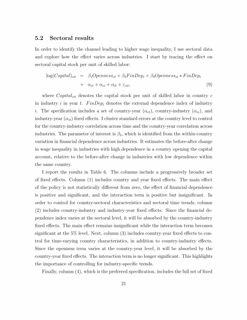
log(Capital)cit = β1Opennessct + β2FinDepi + β3Opennessct ∗ FinDepi+ αct + αci + αit + εcit, (9)

where Capitalcit denotes the capital stock per unit of skilled labor in country c

in industry i in year t. FinDepi denotes the external dependence index of industry

i. The specification includes a set of country-year (αct), country-industry (αci), and

industry-year (αit) fixed effects. I cluster standard errors at the country level to control

for the country-industry correlation across time and the country-year correlation across

industries. The parameter of interest is β3, which is identified from the within-country

variation in financial dependence across industries. It estimates the before-after change

in wage inequality in industries with high dependence in a country opening the capital

account, relative to the before-after change in industries with low dependence within

the same country.

I report the results in Table 6. The columns include a progressively broader set

of fixed effects. Column (1) includes country and year fixed effects. The main effect

of the policy is not statistically different from zero, the effect of financial dependence

is positive and significant, and the interaction term is positive but insignificant. In

order to control for country-sectoral characteristics and sectoral time trends, column

(2) includes country-industry and industry-year fixed effects. Since the financial de-

pendence index varies at the sectoral level, it will be absorbed by the country-industry

fixed effects. The main effect remains insignificant while the interaction term becomes

significant at the 5% level. Next, column (3) includes country-year fixed effects to con-

trol for time-varying country characteristics, in addition to country-industry effects.

Since the openness term varies at the country-year level, it will be absorbed by the

country-year fixed effects. The interaction term is no longer significant. This highlights

the importance of controlling for industry-specific trends.

Finally, column (4), which is the preferred specification, includes the full set of fixed

21

effects. The effect is statistically and economically significant. In order to calculate

the magnitude of the effect, consider an industry at the 75th percentile of the external

financial index (0.475) and an industry at the 25th percentile (-0.343). From Equation

(9), the differential effect across sectors of a one-standard-deviation increase in the

openness index is β3 ∗ (FinDep75th − FinDep25th). According to column (4), capital

opening increases the capital stock in industries that are highly dependent on external

finance by 10% more than in industries with low dependence.22 The standard deviation

of the sectoral (log) capital stock after controlling for country, sector, and year effects is

27%. Since the differential effect is 10%, capital opening explains 37% of the variation

in sectoral capital (=10%/27%).


Next, I analyze the effect on sectoral wage inequality. I divide the sample into

industries with external financial dependence above and below the median of the index

across all industries. For each subset of industries, I estimate:

log(Inequality)cit = β1Opennessct + β2Compi + β3Opennessct ∗ Compi+ αct + αci + αit + εcit, (10)

where Inequalitycit denotes the relative wages of skilled and unskilled workers in

country c in industry i in year t. Comp denotes the capital-skill complementarity in-

dex of industry i. Table 7 reports the results. As in Table 6, the columns include a

progressively broader set of fixed effects. Panel A includes the sample of industries

with dependence above the median and Panel B contains industries below the median.

Within above-median dependence industries, opening increases wage inequality par-

ticularly in industries with strong complementarity (Panel A). The double interaction

term is significant across specifications. Within below-median dependence industries,

the effect is the same across sectors with different degrees of complementarity (Panel

B). This confirms that if the “capital effect” is absent, there is no “complementarity

effect.”

22The differential effect is computed as 0.123*[0.475-(-0.343)]=10%.

22

In order to calculate the magnitude of the effect, consider an industry at the

75th percentile of the complementarity index (0.336) and one at the 25th percentile

(-0.039). From Equation (10), the differential effect of capital account opening is

β3 ∗ (Comp75th − Comp25th). According to column (4) of Panel A, capital opening in-

creases wage inequality in industries with strong complementarity by 3% more than in

industries with weak complementarity.23 The standard deviation of sectoral (log) wage

inequality after controlling for country, sector, and year effects is 14%. This means

that capital opening explains 21% of the variation in sectoral inequality (=3%/14%).

Thus, the economic magnitude of the effect is sizable.


Finally, as an alternative to splitting the sample, I pool all industries and estimate

a triple difference-in-differences specification:

log(Inequality)cit = β1Opennessct + β2Compi + β3FinDepi + β4Opennessct ∗ Compi+ β5Opennessct ∗ FinDepi + β6Opennessct ∗ Compi ∗ FinDepi+ αct + αci + αit + εcit. (11)

The parameter of interest is β6, which is identified from the within-country variation

in both external dependence and complementarity across industries. The coefficients of

the double interaction terms, unlike the triple interaction term, are not scale invariant.

That is, they depend on the units in which the sectoral indices are measured. Table

8 shows that the triple interaction term is significant across all specifications. From

Equation (11), the differential effect of capital opening is β6 ∗ (Comp ∗ FinDep75th −Comp ∗ FinDep25th). As seen in column (3), opening increases wage inequality in

industries with high dependence and strong complementarity (75th percentile in the

product of both indices) by almost 2% more than in industries with low dependence

and weak complementarity (25th percentile).24


23I calculate the differential effect as 0.080*[0.336-(-0.039)]=3%.24I rank all industries according to the product of both sectoral indices. The 75th and 25th percentile

of this product is 0.107 and -0.025, respectively. The differential effect is 0.135*[0.107-(-0.025)]=1.8%.

23

6 Additional results

This section provides a series of additional results that further support the main find-

ings of the paper.

6.1 Levels of wages

In the previous section, I provided evidence that opening the capital account leads

to higher wage inequality. This can be the result of two alternative scenarios. First,

wages of both skilled and unskilled workers are increasing but skilled wages increase

at a higher rate. Second, skilled wages are increasing while unskilled wages decrease.

From a policy perspective, it is important to disentangle both scenarios. In this section,

I estimate the effect of capital opening on the level of wages.

In particular, I re-estimate Equation (7) separately for skilled wages, unskilled

wages, and overall wages. Table 9 reports the results. According to column (1), capital

opening increases the wages of skilled workers by 2.1%. As seen in column (2), opening

decreases unskilled wages by 2.5%. In column (3), I estimate the impact on the average

wage, which is defined as the weighted average of skilled and unskilled wages, where

the weights are the relative number of skilled and unskilled workers. According to

the results, opening increases overall wages by 1.2%. In sum, opening the capital

account increases overall wages, which is consistent with the evidence provided by

Chari et al. (2012). However, skilled wages increase at the expense of unskilled wages,

which leads to higher wage inequality. As a result, the distributional consequences of

capital opening should be an important concern for policy makers.


6.2 Stability of effect over time

Given that the sample period under study is relatively long (1975-2005), I analyze

whether the relationship between capital account opening and wage inequality docu-

mented in the previous section varies over time. To do this, I add an interaction term

between the capital openness index and a dummy indicator for different decades to

24

Equation (7). The results are reported in Table 10. In column (1), I add an interaction

term between capital account opening and a post-opening dummy equal to one after

1980 and zero otherwise. In columns (2) and (3), I replicate the exercise using a post

dummy for 1990 and 2000. In column (4), I include all three post dummies simultane-

ously. According to the results, the effect of capital account opening on wage inequality

remains unchanged across all specifications. The coefficients for all post dummies are

not significant.


6.3 Reverse causality

As discussed in Section 3, the fact that capital opening is not exogenous can lead

to a problem of reverse causality. In this section, I address this issue by using an

instrumental variables approach. Several papers studying the effect of opening on

growth have used some type of instrumental variables analysis to deal with endogeneity.

The instruments used range from legal origin to distance to the equator. The problem is

that these instruments do not have a time-series dimension. To address this problem,

I follow the work of Quinn and Toyoda (2008) and use lagged values of the capital

openness index as internal instruments.

I estimate Equation (11) in first differences using GMM. I use the following moment

conditions: E[zcit−j · ∆εcit] = 0 for j ≥ 2, t ≥ 3, where z = [Inequality, Openness,

Openness ∗ Comp]. The identification assumption is that the error term in Equation

(11) is not serially correlated and that the explanatory variables are weakly exogenous.

Intuitively, I assume that lagged values of the openness index affect wage inequality only

through their effect on current openness. Table 11 reports the results. According to the

results of column (4), the triple interaction term is positive and significant. The size

of the coefficient (0.158) is very similar to the size of the coefficient of the benchmark

estimation of Table 8 (0.135). This finding provides further evidence against a reverse

causality story.


25

6.4 Alternative explanations

A potential confounding factor is trade liberalization. According to the Stolper-

Samuelson Theorem, trade opening increases the relative price of a country’s abundant

factor. Given that my sample is composed of more-developed (and skill-abundant)

countries, simultaneous changes in trade policy might increase the relative wage of

skilled labor.25 In order to control for trade opening in the sectoral analysis, I re-

estimate Equation (11) and control for trade openness and its interaction with the

two sectoral indices. I use two alternative measures of trade: the ratio of exports and

imports to GDP and the simple mean applied tariff. I report the results in columns

(1) and (2) of Table 12.26 The table shows that the triple interaction term of capital

opening remains unchanged. The triple interaction term using either trade opening

measure is not statistically significant.

Another alternative story is that capital account opening went hand in hand with

financial sector liberalization. According to Kneer (2013), financial liberalization and

the consequent financial sector growth increases the demand for highly skilled workers,

which in turn increases the wage gap between skilled and unskilled labor. In order to

rule out this possibility, I re-estimate Equation (11) and control for financial liberaliza-

tion and its interaction with the two sectoral characteristics. I use the same measure of

financial liberalization as Kneer (2013), which is based on an index provided by Abiad

et al. (2010).27 The results are reported in column (3) of Table 12. Even though the

triple interaction term of financial liberalization is statistically significant, the triple

interaction term of capital account opening barely changes. In sum, my results are not

driven by either trade or financial sector liberalization.

A final alternative story is that capital opening induces skill-intensive firms to

expand. This would change the within-industry composition of firms toward more skill-

25In addition, since reductions in trade costs make it cheaper to import capital equipment, tradeopenness can lead to higher wage inequality through capital deepening and capital-skill complemen-tarity (Parro, 2013; Raveh and Reshef, 2014).

26To preserve space, all estimations from here onward include the full set of fixed effects.27The index takes into account seven different components of financial reform: credit controls,

interest rate controls, barriers to entry into the financial sector, state ownership of banks, securitiesmarket policies, banking regulation and supervision, and capital account restrictions. Since my focusis on capital account opening, I subtract the last component from the overall index.

26

intensive firms, increasing the relative demand for skilled labor. This compositional

effect could lead to higher wage inequality, even if firms do not exhibit capital-skill

complementarity. In Section A.4 of the online appendix, I use firm-level data from an

emerging market and provide evidence against this between-firm composition channel

(see Table A.6).


6.5 Robustness checks

Different capital openness measures. I show that the results are robust to using

alternative capital account openness indicators. First, I use three de jure measures.

The Quinn (1997) index scores the intensity of controls for capital account receipts

and capital account payments separately. Abiad et al. (2010) take into account restric-

tions on capital inflows, capital outflows, and unification of the exchange rate system.

Kaminsky and Schmukler (2008) create an index based on restrictions on borrowing

abroad. Finally, I use the de facto measure of financial integration developed by Lane

and Milesi-Ferretti (2007), which equals the sum of foreign assets and liabilities as

a fraction of GDP. Table 13 reports the results (columns 1-4). Each column shows

the results for a different capital openness measure. The triple interaction term is

statistically significant across all measures.


Different measures of complementarity. In Section 4, I estimated the capital-

skill complementarity index using data for the whole sample period 1975-2005. This

allows me to maximize the number of observations per estimation. However, since the

index is calculated with post-opening data, it is not fully exogenous. To address this

issue, I provide two alternative measures of the complementarity index. First, I re-

estimate the index using only pre-opening data. As before, I obtain a precise opening

date by defining the opening year as the year in which a country’s capital openness

index increases by more than one standard deviation. Second, I re-estimate the index

using data prior to 1990. In addition, I re-estimate the index excluding the transition

27

economies. The idea is to exclude the countries presenting the most distortions and

frictions. Table 13 (columns 5-7) shows the results of estimating Equation (11) using

these alternative indices. The results remain statistically significant.

Others. In Section A.5 of the online appendix, I show that the differential effect

of capital account opening across industries is particularly strong for older workers

and female workers (see Table A.7). Since these workers have relatively low sectoral

mobility, this result highlights the importance of imperfect industry mobility for the

sectoral analysis. Finally, in Section A.6 of the online appendix, I re-estimate the

sectoral regressions excluding the most developed countries from the sample. According

to the analysis (see Table A.8), the results are driven by the less-developed, capital-

scarce economies of the sample.

7 Conclusions

Capital account opening affects both economic growth and income inequality. While

economists have thoroughly studied the effects of capital liberalization on growth, the

potentially enormous impact of such a policy on inequality has been underappreciated.

The three volumes of the Handbook of Income Distribution, for example, do not mention

any possible connections between inequality and capital account policy. In this paper,

I provide evidence that capital account opening increases wage inequality in a sample

of 20 primarily European countries from 1975-2005.

I conduct a two-fold empirical strategy. First, I use aggregate data and exploit the

variation in the timing of capital account openings across countries. Second, I focus on

a specific mechanism, which works through technology embodied in the capital stock.

When capital and skilled labor are relative complements, the capital that financially-

constrained firms raise from abroad increases the relative demand for skilled labor.

This enlarges the wage gap between skilled and unskilled workers. The effect should

be stronger for firms in industries that are heavily dependent on external finance and

for firms in industries with strong complementarity between capital and skills. To iden-

tify the mechanism, I use sectoral data and exploit the variation in external financial

dependence and complementarity across sectors.

28

I find that capital opening increases aggregate wage inequality by 5%, which ex-

plains 18% of the variation in aggregate wage inequality after accounting for fixed

effects. Regarding the mechanism, I find that opening the capital account increases

the capital stock in industries with high financial dependence by 10% more than in

industries with low dependence. Within above-median dependence industries, opening

increases wage inequality in industries with strong complementarity by 3% more than

in industries with weak complementarity. This explains 21% of the variation in sectoral

wage inequality after accounting for fixed effects. Within below-median dependence

industries, the effect is uniform across sectors with different degrees of complementarity.

This paper’s findings can be extended in several directions. First, the results are

driven by a relatively small set of more-developed countries, which may not be repre-

sentative of a larger set of countries. It would be interesting to extend the analysis to a

broader group of more capital-scarce emerging markets. Second, since the mechanism

examined in this paper works within a firm, it would be useful to conduct a firm-level

analysis, using a cross-country firm-level dataset. Finally, this paper focuses exclusively

on one aspect of income inequality, the wage gap between skilled and unskilled workers.

Capital market integration could also affect cross-dynastic income differences through

human capital accumulation. Extending the analysis to other inequality dimensions

represents an interesting direction for further research.

29

References

Abiad, A., Detragiache, E., and Tressel, T. (2010). A new database of financial reforms.

IMF Staff Papers, 57(2):281–302.

Alfaro, L., Chanda, A., Kalemli-Ozcan, S., and Sayek, S. (2004). FDI and economic

growth: The role of local financial markets. Journal of International Economics,

64(1):89–112.

Alfaro, L. and Hammel, E. (2007). Capital flows and capital goods. Journal of Inter-

national Economics, 72(1):128–150.

Beck, T., Demirg-Kunt, A., and Levine, R. (2007). Finance, inequality and the poor.

Journal of Economic Growth, 12(1):27–49.

Beck, T., Levine, R., and Levkov, A. (2010). Big bad banks? The winners and losers

from bank deregulation in the United States. Journal of Finance, 65(5):1637–1667.

Bekaert, G., Harvey, C. R., and Lundblad, C. (2005). Does financial liberalization spur

growth? Journal of Financial Economics, 77(1):3–55.

Berman, E., Bound, J., and Griliches, Z. (1994). Changes in the demand for skilled

labor within US manufacturing: Evidence from the annual survey of manufacturers.

Quarterly Journal of Economics, 109(2):367–397.

Bertrand, M., Duflo, E., and Mullainathan, S. (2004). How much should we trust

differences-in-differences estimates? Quarterly Journal of Economics, 119(1):249–

275.

Chari, A., Henry, P. B., and Sasson, D. (2012). Capital market integration and wages.

American Economic Journal: Macroeconomics, 4(2):102–32.

Chinn, M. D. and Ito, H. (2006). What matters for financial development? Cap-

ital controls, institutions, and interactions. Journal of Development Economics,

8(1):163–192.

Das, M. and Mohapatra, S. (2003). Income inequality: The aftermath of stock market

liberalization in emerging markets. Journal of Empirical Finance, 10(1-2):217–248.

Duffy, J., Papageorgiou, C., and Perez-Sebastian, F. (2004). Capital-skill complemen-

30

tarity? Evidence from a panel of countries. Review of Economics and Statistics,

86(1):327–344.

Edwards, S. (2001). Capital mobility and economic performance: Are emerging

economies different? NBER Working Paper, No. w8076.

Griliches, Z. (1969). Capital-skill complementarity. Review of Economics and Statistics,

51(4):465–468.

Gupta, N. and Yuan, K. (2009). On the growth effect of stock market liberalizations.

Review of Financial Studies, 22(11):4715–4752.

Helwege, J. (1992). Sectoral shifts and interindustry wage differentials. Journal of

Labor Economics, 10(1):55–84.

Henry, P. B. (2000). Do stock market liberalizations cause investment booms? Journal

of Financial Economics, 58(1-2):301–334.

Imbens, G. W. and Wooldridge, J. M. (2009). Recent developments in the econometrics

of program evaluation. Journal of Economic Literature, 47(1):5–86.

Jerzmanowski, M. and Nabar, M. (2013). Financial development and wage inequality:

Theory and evidence. Economic Inquiry, 51(1):211–234.

Kaminsky, G. L. and Schmukler, S. (2008). Short-run pain, long-run gain: Financial

liberalization and stock market cycles. Review of Finance, 12(2):253–292.

Katz, L. F. and Autor, D. H. (1999). Changes in the wage structure and earnings

inequality. volume 3 of Handbook of Labor Economics, chapter 26, pages 1463–1555.

Katz, L. F. and Murphy, K. M. (1992). Changes in relative wages, 1963-1987: Supply

and demand factors. Quarterly Journal of Economics, 107(1):35–78.

Klein, M. and Olivei, G. (2008). Capital account liberalization, financial depth, and

economic growth. Journal of International Money and Finance, 27(6):861–875.

Kneer, C. (2013). Finance as a magnet for the best and brightest: Implications for the

real economy. DNB Working Paper, No. 392.

Krusell, P., Ohanian, L. E., Rios-Rull, J.-V., and Violante, G. L. (2000). Capital-

skill complementarity and inequality: A macroeconomic analysis. Econometrica,

31

68(5):1029–1053.

Lane, P. R. and Milesi-Ferretti, G. M. (2007). The external wealth of nations mark II:

Revised and extended estimates of foreign assets and liabilities, 1970-2004. Journal

of International Economics, 73(2):223–250.

Parro, F. (2013). Capital-skill complementarity and the skill premium in a quantitative

model of trade. American Economic Journal: Macroeconomics, 5(2):72–117.

Quinn, D. P. (1997). The correlates of change in international financial regulation.

American Political Science Review, 91(3):531–551.

Quinn, D. P. and Toyoda, A. M. (2008). Does capital account liberalization lead to

growth? Review of Financial Studies, 21(3):1403–1449.

Rajan, R. G. and Zingales, L. (1998). Financial dependence and growth. American

Economic Review, 88(3):559–586.

Raveh, O. and Reshef, A. (2014). Capital imports composition, complementarities,

and the skill premium in developing countries. Mimeo, University of Virginia.

Violante, G. (2006). Skill-biased technical change. In Blume, L. and Durlauf, S.,

editors, The New Palgrave Dictionary of Economics. Palgrave Macmillan.

32

Figure 1: Dynamic Effect of Capital Account Opening on Aggregate WageInequality

-.03

0.0

3.0

6.0

9Pe

rcen

tage

Cha

nge

in S

kill P

rem

ium

-6 -4 -2 0 2 4 6 8 10Years Relative to Capital Account Opening

Notes: the figure plots the dynamic impact of capital account opening on aggregate wage inequality. In order to obtaina precise opening date, I define the opening year as the year in which the Chinn and Ito (2006) openness index of acountry increases by more than one standard deviation. I consider a 15-year window, spanning from 5 years beforeopening until 10 years after opening. I exclude the year of opening, thus estimating the dynamic effect of capitalaccount opening relative to that year. The dashed lines denote 95% confidence intervals, where standard errors havebeen clustered at the country level.

33

Table 1: Summary Statistics of Capital Account Openness Index

(1) (2) (3) (4) (5)Mean Median StdDev. Min. Max.

Australia 1.245 1.132 1.041 -0.106 2.456Austria 1.687 1.132 0.628 1.132 2.456Belgium 1.471 1.662 0.860 0.521 2.456Czech Republic 1.042 0.910 1.180 -0.106 2.456Denmark 1.296 1.926 1.235 -0.106 2.456Finland 1.647 1.132 0.700 -0.106 2.456France 0.977 0.158 1.288 -1.159 2.456Greece -0.147 -1.159 1.327 -1.159 2.456Hungary -0.368 -0.633 1.534 -1.856 2.456Ireland 0.858 -0.106 1.302 -0.803 2.456Italy 0.616 0.158 1.735 -1.856 2.456Japan 2.157 2.456 0.472 1.132 2.456Korea -0.548 -0.106 0.528 -1.159 -0.106Poland -1.120 -1.159 0.768 -1.856 0.079Portugal 0.441 -0.106 1.623 -1.159 2.456Slovakia -0.629 -1.159 0.863 -1.159 0.873Slovenia 0.690 1.132 0.993 -1.159 1.926Spain 0.772 -0.106 1.254 -1.159 2.456Sweden 1.602 1.132 0.606 1.132 2.456United Kingdom 1.950 2.456 1.105 -0.803 2.456

All countries 0.894 1.132 1.398 -1.856 2.456

Notes: the table reports summary statistics for the capital account openness index for the 20 countries in the sampleduring the period 1975-2005. The openness index comes from Chinn and Ito (2006). The last row reports the statisticsfor the average across all countries. Column (1) reports the mean; Column (2) the median; Column (3) the standarddeviation; Column (4) the minimum; and Column (5) the maximum.

34

Table 2: Summary Statistics of Aggregate Wage Inequality

(1) (2) (3) (4) (5)Mean Median StdDev. Min. Max.

Australia 1.490 1.467 0.044 1.440 1.593Austria 1.577 1.582 0.075 1.476 1.729Belgium 1.502 1.507 0.031 1.438 1.557Czech Republic 2.263 2.246 0.033 2.226 2.319Denmark 1.492 1.498 0.084 1.384 1.633Finland 1.652 1.593 0.125 1.504 1.885France 1.849 1.851 0.074 1.620 1.949Greece 1.552 1.540 0.035 1.505 1.626Hungary 2.404 2.451 0.110 2.200 2.547Ireland 1.826 1.844 0.066 1.690 1.922Italy 1.264 1.254 0.099 1.133 1.480Japan 1.673 1.662 0.045 1.608 1.757Korea 1.780 1.753 0.217 1.491 2.123Poland 1.558 1.560 0.027 1.511 1.600Portugal 2.307 2.322 0.106 2.118 2.430Slovakia 1.785 1.775 0.068 1.692 1.905Slovenia 2.119 2.119 0.057 2.031 2.215Spain 1.558 1.587 0.112 1.356 1.707Sweden 1.522 1.529 0.041 1.435 1.604United Kingdom 1.829 1.841 0.076 1.574 1.942

All countries 1.687 1.611 0.275 1.133 2.547

Notes: the table reports summary statistics for aggregate wage inequality for the 20 countries in the sample duringthe period 1975-2005. Wage inequality is defined as the relative wage between workers with college and high-schooleducation. The last row reports the statistics for the average across all countries. Column (1) reports the mean; Column(2) the median; Column (3) the standard deviation; Column (4) the minimum; and Column (5) the maximum.

35

Table 3: Sectoral Index of External Financial Dependence

(1) (2)Industry Industry Ext. Financialname ISIC code Dependence

Manufacturing of wood 20 0.283Manufacturing of coke, refined petroleum 23 0.694Manufacturing of chemicals 24 1.000Manufacturing of rubber, plastics 25 0.296Manufacturing of non-metallic mineral products 26 0.380Manufacturing of machinery and equipment 29 0.269Construction 45 -0.228Sale, maintenance, repair motor vehicles 50 -0.475Wholesale trade and commission trade 51 -0.399Retail trade, except of motor vehicles 52 0.065Hotels and restaurants 55 0.370Post and telecommunications 64 0.476Real estate activities 70 0.511Education 80 -0.383Health and social work 85 -0.344

Notes: the table reports the external financial dependence index for the 15 two-digit industries in the sample. Externalfinancial dependence is defined as the fraction of capital expenditures not financed by cash flow from operations (Rajanand Zingales, 1998). The index is calculated as the median of this fraction across US publicly traded firms for eachindustry.

36

Tab

le4:

Sect

ora

lIn

dex

of

Capit

al-

skil

lC

om

ple

menta

rity

(1)

(2)

(3)

(4)

(5)

(6)

Ind

ust

ryIn

du

stry

Coeff

.S

tdD

ev.

Coeff

.S

tdD

ev.

Nu

mb

erof

Nam

eIS

ICco

de

Bet

aB

eta

Gam

ma

Gam

ma

Ob

serv

ati

on

s(C

SC

ind

ex)

Man

ufa

ctu

rin

gof

wood

20

0.5

22***

0.0

67

0.0

73**

0.0

34

303

Man

ufa

ctu

rin

gof

coke

,re

fin

edp

etro

leu

m23

1.1

89***

0.0

94

0.0

49***

0.0

15

303

Man

ufa

ctu

rin

gof

chem

ical

s24

1.3

05***

0.0

78

0.2

14***

0.0

41

303

Man

ufa

ctu

rin

gof

rub

ber

,pla

stic

s25

0.2

88***

0.0

86

0.3

65***

0.0

36

303

Man

ufa

ctu

rin

gof

non

-met

alli

cm

iner

alp

rod

uct

s26

0.8

39***

0.0

99

0.3

02***

0.0

35

303

Man

ufa

ctu

rin

gof

mac

hin

ery

and

equ

ipm

ent

29

0.6

06***

0.0

82

0.0

44*

0.0

23

303

Con

stru

ctio

n45

1.2

31***

0.1

14

0.1

34***

0.0

36

303

Sal

e,m

ainte

nan

ce,

rep

air

mot

orveh

icle

s50

0.2

79***

0.0

30.3

78***

0.0

24

303

Wh

oles

ale

trad

ean

dco

mm

issi

ontr

ade

51

1.8

95***

0.0

86

0.3

36***

0.0

39

303

Ret

ail

trad

e,ex

cep

tof

mot

orve

hic

les

52

2.2

58***

0.0

74

-0.0

88***

0.0

32

303

Hot

els

and

rest

aura

nts

55

1.2

87***

0.0

58

0.0

37

0.0

41

303

Pos

tan

dte

leco

mm

un

icat

ion

s64

1.1

92***

0.0

79

0.4

70***

0.0

4303

Rea

les

tate

acti

vit

ies

70

1.7

55***

0.0

50

-0.0

50.0

36

303

Ed

uca

tion

80

0.7

66***

0.0

53

-0.0

70***

0.0

13

303

Hea

lth

and

soci

alw

ork

85

0.6

96***

0.0

61

-0.0

39*

0.0

21

303

Note

s:th

eta

ble

rep

ort

sth

ees

tim

ate

sof

the

skille

dla

bor

share

equ

ati

on

for

each

of

the

15

two-d

igit

ind

ust

ries

inth

esa

mp

le.

Colu

mn

s(2

)an

d(3

)re

port

the

coeffi

cien

tan

dst

an

dard

dev

iati

on

of

the

elast

icit

yof

the

share

of

wages

paid

tosk

ille

dla

bor

wit

hre

spec

tto

rela

tive

wages

;C

olu

mn

s(4

)an

d(5

)re

port

the

coeffi

cien

tan

dst

an

dard

dev

iati

on

of

the

elast

icit

yw

ith

resp

ect

toca

pit

alin

ten

sity

.T

he

coeffi

cien

tof

colu

mn

(4)

corr

esp

on

ds

toth

eca

pit

al-

skillco

mp

lem

enta

rity

ind

ex.

Sta

nd

ard

erro

rsare

clu

ster

edat

the

cou

ntr

yle

vel

.***,

**,

*d

enote

stati

stic

al

sign

ifica

nce

at

1%

,5%

,an

d10%

.

37

Table 5: Effect of Capital Account Opening on Aggregate Wage Inequality

(1) (2) (3) (4)

Capital Openness 0.064*** 0.057*** 0.050***(0.010) (0.009) (0.010)

Post 0.048***(0.013)

Relative Supply -0.148*** -0.148*** -0.152***(0.033) (0.031) (0.032)

Inflation -0.011 -0.009 -0.009(0.007) (0.007) (0.007)

Gov. Exp. to GDP -0.068*** -0.059*** -0.045**(0.017) (0.019) (0.019)

GDP per Capita -0.113*** -0.108*** -0.128***(0.017) (0.016) (0.017)

Credit to GDP 0.052*** 0.052*** 0.050***(0.012) (0.012) (0.012)

Trade Openness 0.017 0.041(0.025) (0.026)

Fin. Liberalization 0.044*** 0.057***(0.014) (0.014)

Fixed EffectsCountry Yes Yes Yes YesYear Yes Yes Yes Yes

Observations 381 369 369 370R-squared 0.899 0.926 0.928 0.923

Notes: the table reports the estimates of the effect of capital account opening on aggregate wage inequality. Column(1) estimates the effect without controls; Column (2) controls for the relative supply of skilled labor, inflation, ratio ofgovernment expenditure to GDP, GDP per capita, ratio of private credit to GDP; Column (3) further controls for tradeand financial liberalization; Column (4) replaces the capital openness variable with a dummy variable equal to one afterthe openness index of a country increases by more than one standard deviation and zero otherwise. Standard errors inparentheses are clustered at the country level. ***, **, * denote statistical significance at 1%, 5%, and 10%.

38

Table 6: Effect of Capital Account Opening on Sectoral Capital Stock

(1) (2) (3) (4)

Capital Openness 0.033 0.044(0.053) (0.058)

Fin. Dep. 0.064***(0.003)

Capital Openness * Fin. Dep. 0.058 0.123** 0.058 0.123**(0.046) (0.051) (0.047) (0.053)

Fixed effectsCountry Yes No No NoYear Yes No No NoCountry-year No No Yes YesCountry-industry No Yes Yes YesIndustry-year No Yes No Yes

Observations 4,095 4,095 4,095 4,095R-squared 0.575 0.975 0.981 0.982

Notes: the table reports the estimates of the effect of capital account opening on the sectoral capital stock per unit ofskilled labor. Column (1) includes country and year fixed effects; Column (2) includes country-industry and industry-year fixed effects; Column (3) includes country-year and country-industry fixed effects; Column (4) includes country-year,country-industry, and sector-year fixed effects. Fin. Dep. stands for external financial dependence. Standard errors inparentheses are clustered at the country level. ***, **, * denote statistical significance at 1%, 5%, and 10%.

39

Table 7: Effect of Capital Account Opening on Sectoral Wage Inequality:Sub-sample Analysis

(1) (2) (3) (4)

A. Above-median financialdependence industries


Comp. -0.089(0.052)

Capital Openness * Comp. 0.042 0.080* 0.098** 0.080*(0.039) (0.043) (0.042) (0.046)


B. Below-median financialdependence industries


Comp. 0.209**(0.085)

Capital Openness * Comp. -0.077 -0.019 -0.040 -0.019(0.048) (0.035) (0.026) (0.038)



Notes: the table reports the estimates of the effect of capital account opening on sectoral wage inequality. Panel Acontains the sub-sample of above-median external financial dependence industries; Panel B the sub-sample of below-median dependence industries. Column (1) includes country and year fixed effects; Column (2) includes country-industryand industry-year fixed effects; Column (3) includes country-year and country-industry fixed effects; Column (4) includescountry-year, country-industry, and sector-year fixed effects. Comp. stands for capital-skill complementarity. Standarderrors in parentheses are clustered at the country level. ***, **, * denote statistical significance at 1%, 5%, and 10%.

40

Table 8: Effect of Capital Account Opening on Sectoral Wage Inequality

(1) (2) (3) (4)


Fin. Dep. -0.019*(0.011)

Comp. 0.189***(0.022)

Capital Openness * Fin. Dep. -0.047* -0.026 -0.047* -0.026(0.026) (0.027) (0.027) (0.028)

Capital Openness * Comp. 0.013 0.022 0.013 0.022(0.022) (0.028) (0.023) (0.029)

Capital Openness * Fin. Dep. * Comp. 0.192*** 0.135* 0.192** 0.135*(0.066) (0.072) (0.068) (0.074)



Notes: the table reports the estimates of the effect of capital account opening on sectoral wage inequality. Column (1)includes country and year fixed effects; Column (2) includes country-industry and industry-year fixed effects; Column (3)includes country-year and country-industry fixed effects; Column (4) includes country-year, country-industry, and sector-year fixed effects. Fin. Dep. stands for external financial dependence and Comp. for capital-skill complementarity.Standard errors in parentheses are clustered at the country level. ***, **, * denote statistical significance at 1%, 5%,and 10%.

41

Table 9: Effect of Capital Account Opening on Level of Wages

(1) (2) (3)Skilled Unskilled AverageWages Wages Wages

Capital Openness 0.021*** -0.025*** 0.012*(0.006) (0.009) (0.007)

Relative Supply 0.023 0.039 0.062*(0.028) (0.029) (0.032)

Trade Openness -0.002 -0.037* 0.006(0.014) (0.020) (0.013)

Inflation -0.034*** -0.020*** -0.019***(0.006) (0.007) (0.006)

Gov. Exp. to GDP -0.010 0.027* 0.034***(0.013) (0.016) (0.012)

GDP per Capita -0.132*** -0.124*** -0.144***(0.007) (0.012) (0.007)

Credit to GDP -0.003 -0.059*** -0.035***(0.007) (0.009) (0.007)

Fin. Liberalization -0.029** -0.034** -0.035***(0.013) (0.014) (0.012)

Fixed EffectsCountry Yes Yes YesYear Yes Yes Yes

Observations 369 338 338R-squared 0.997 0.997 0.998

Notes: the table reports the estimates of the effect of capital account opening on the level of wages. Column (1)estimates the effect for the level of skilled wages; Column (2) for unskilled wages; Column (3) for the average wage,which is defined as the weighted average of skilled and unskilled wages, where the weights are given by the relativenumber of workers by skill level. Standard errors in parentheses are clustered at the country level. ***, **, * denotestatistical significance at 1%, 5%, and 10%.

42

Table 10: Effect of Capital Account Opening on Aggregate WageInequality: Stability Over Time

(1) (2) (3) (4)

Capital Openness 0.060*** 0.052*** 0.051*** 0.059***(0.018) (0.015) (0.009) (0.019)

Capital Openness * Post1980 -0.013 -0.015(0.019) (0.019)

Capital Openness * Post1990 -0.003 0.005(0.016) (0.016)

Capital Openness * Post2000 -0.004 -0.004(0.012) (0.012)

Relative Supply -0.152*** -0.149*** -0.150*** -0.153***(0.031) (0.031) (0.033) (0.032)

Trade Openness 0.020 0.018 0.017 0.019(0.025) (0.025) (0.025) (0.025)

Inflation -0.011 -0.010 -0.009 -0.010(0.007) (0.007) (0.007) (0.007)

Gov. Exp. to GDP -0.061*** -0.060*** -0.060*** -0.061***(0.019) (0.019) (0.019) (0.019)

GDP per Capita -0.111*** -0.109*** -0.110*** -0.111***(0.017) (0.019) (0.017) (0.019)

Credit to GDP 0.054*** 0.052*** 0.052*** 0.054***(0.013) (0.013) (0.012) (0.013)

Fin. Liberalization 0.043*** 0.044*** 0.044*** 0.043***(0.014) (0.014) (0.014) (0.014)

Fixed EffectsCountry Yes Yes Yes YesYear Yes Yes Yes Yes

Observations 369 369 369 369R-squared 0.928 0.927 0.927 0.927

Notes: the table reports the estimates of the effect of capital account opening on aggregate wage inequality for differenttime periods. Columns (1), (2), and (3) include an interaction term between the capital openness index and a dummyequal to one after 1980, 1990, 2000 and zero otherwise, respectively; Column (4) includes all three interaction termssimultaneously. Standard errors in parentheses are clustered at the country level. ***, **, * denote statistical significanceat 1%, 5%, and 10%.

43

Table 11: Effect of Capital Account Opening on Sectoral Wage Inequality:Instrumental Variable Approach

(1) (2) (3) (4)


Capital Openness* Fin. Dep. -0.014 -0.039*** -0.036*** -0.088***(0.014) (0.005) (0.005) (0.011)

Capital Openness * Comp. -0.013 -0.016** 0.006 -0.139***(0.020) (0.008) (0.006) (0.025)

Capital Openness * Fin. Dep. * Comp. 0.098* 0.192*** 0.151*** 0.158***(0.058) (0.019) (0.018) (0.033)


Observations 6,180 6,180 6,180 6,180

Notes: the table reports the estimates of the effect of capital account opening on sectoral wage inequality, usinglagged values of the capital openness index as internal instrumental variables. Column (1) includes country and yearfixed effects; Column (2) includes country-industry and industry-year fixed effects; Column (3) includes country-yearand country-industry fixed effects; Column (4) includes country-year, country-industry, and sector-year fixed effects.Fin. Dep. stands for external financial dependence and Comp. for capital-skill complementarity. Standard errors inparentheses are clustered at the country level. ***, **, * denote statistical significance at 1%, 5%, and 10%.

44

Table 12: Effect of Capital Account Opening on Sectoral Wage Inequality:Controlling for Trade and Financial Liberalization

(1) (2) (3)Trade Average Financial

Openness Tariff Liberalization

Capital Openness * Fin. Dep. -0.027 -0.023*** -0.027***(0.023) (0.008) (0.009)

Capital Openness * Comp. 0.038 0.018 0.033***(0.033) (0.016) (0.012)

Capital Openness * Fin. Dep. * Comp. 0.150* 0.074* 0.152***(0.085) (0.040) (0.037)

Trade Openness * Fin. Dep. 0.005(0.032)

Trade Openness * Comp. -0.026(0.047)

Trade Openness * Fin. Dep. * Comp. -0.077(0.120)

Average Tariff * Fin. Dep. 0.002(0.007)

Average Tariff * Comp. 0.001(0.007)

Average Tariff * Fin. Dep.* Comp. -0.009(0.014)

Fin. Liberalization * Fin. Dep. 0.000(0.010)

Fin. Liberalization * Comp. 0.019(0.018)

Fin. Liberalization * Fin. Dep. * Comp. 0.096**(0.048)

Fixed effectsCountry-year Yes Yes YesCountry-industry Yes Yes YesIndustry-year Yes Yes Yes

Observations 4,440 3,465 4,440R-squared 0.950 0.954 0.950

Notes: the table reports the estimates of the effect of capital account opening on sectoral wage inequality, controlling fortrade and financial liberalization. Columns (1), (2), and (3) control for the interaction between the two sectoral indicesand the ratio of exports and imports to GDP, average import tariff, and financial liberalization index, respectively. Allspecifications include country-year, country-industry, and industry-year fixed effects. Fin. Dep. stands for externalfinancial dependence and Comp. for capital-skill complementarity. Standard errors in parentheses are clustered at thecountry level. ***, **, * denote statistical significance at 1%, 5%, and 10%.

45

Tab

le13:

Eff

ect

of

Capit

al

Acc

ount

Op

enin

gon

Sect

ora

lW

age

Inequ

ali

ty:

Rob

ust

ness

Ch

eck

s

Alt

ern

ativ

eC

ap

ital

Acc

ou

nt

Op

enn

ess

Mea

sure

sA

lter

nati

veC

om

ple

men

tari

tyM

easu

res

(1)

(2)

(3)

(4)

(5)

(6)

(7)

Qu

inn

Ab

iad

Kam

insk

yL

an

eP

re-o

pen

ing

Pre

-1990

No-t

ran

siti

on

Cap

ital

etal.

Sch

mu

kle

rM

iles

i-F

erre

tiC

ap

-skil

lC

ap

-skil

l.C

ap

-skil

lO

pen

nes

sO

pen

nes

sO

pen

nes

sO

pen

nes

sC

om

p.

Com

p.

Com

p.

Ind

exIn

dex

Ind

exIn

dex

Index

Ind

exIn

dex

Cap

ital

Op

enn

ess

*F

in.

Dep

.-0

.033

**-0

.035*

-0.0

38***

-0.0

28**

-0.0

14

-0.0

34*

-0.0

42**

(0.0

15)

(0.0

20)

(0.0

07)

(0.0

13)

(0.0

11)

(0.0

17)

(0.0

18)

Cap

ital

Op

enn

ess

*C

SC

-0.0

04-0

.014

0.0

03

0.0

11

0.0

01

0.0

41*

0.0

13

(0.0

23)

(0.0

18)

(0.0

08)

(0.0

20)

(0.0

43)

(0.0

22)

(0.0

29)

Cap

ital

Op

enn

ess

*E

FD

*C

SC

0.12

7**

0.1

20

0.1

49***

0.1

08**

0.1

82*

0.0

95*

0.2

02**

(0.0

58)

(0.0

71)

(0.0

25)

(0.0

45)

(0.1

02)

(0.0

53)

(0.0

79)

Fix

edeff

ects

Cou

ntr

y-y

ear

Yes

Yes

Yes

Yes

Yes

Yes

Yes

Cou

ntr

y-i

nd

ust

ryY

esY

esY

esY

esY

esY

esY

esIn

du

stry

-yea

rY

esY

esY

esY

esY

esY

esY

es

Ob

serv

atio

ns

5,85

05,7

30

5,0

40

6,5

25

6,4

80

6,4

80

6,4

80

R-s

qu

ared

0.93

90.9

42

0.9

10

0.9

39

0.9

39

0.9

39

0.9

39

Note

s:th

eta

ble

rep

ort

sth

ees

tim

ate

sof

the

effec

tof

cap

ital

acc

ou

nt

op

enin

gon

sect

ora

lw

age

ineq

uality

for

alt

ern

ati

ve

cap

ital

op

enn

ess

mea

sure

san

dca

pit

al-

skill

com

ple

men

tari

tym

easu

res.

Colu

mn

(1)

use

sth

eQ

uin

n(1

997)

op

enn

ess

ind

ex;

Colu

mn

(2)

the

Ab

iad

etal.

(2010)

op

enn

ess

ind

ex;

Colu

mn

(3)

the

op

enn

ess

Kam

insk

yan

dS

chm

ukle

r(2

008)

ind

ex;

Colu

mn

(4)

the

Lan

ean

dM

iles

i-F

erre

tti

(2007)

op

enn

ess

ind

ex;

Colu

mn

(5)

use

sa

com

ple

men

tari

tyin

dex

esti

mate

du

sin

gp

re-o

pen

ing

data

;C

olu

mn

(6)

use

sa

com

ple

men

tari

tyin

dex

esti

mate

du

sin

gp

re-1

990

data

;C

olu

mn

(7)

use

sa

com

ple

men

tari

tyin

dex

esti

mate

dex

clu

din

gtr

an

siti

on

econ

om

ies.

All

spec

ifica

tion

sin

clu

de

cou

ntr

y-y

ear,

cou

ntr

y-i

nd

ust

ry,

an

din

du

stry

-yea

rfi

xed

effec

ts.

All

spec

ifica

tion

sin

clu

de

cou

ntr

y-y

ear,

cou

ntr

y-i

nd

ust

ry,

an

din

du

stry

-yea

rfi

xed

effec

ts.

Fin

.D

ep.

stan

ds

for

exte

rnal

fin

an

cial

dep

end

ence

an

dC

om

p.

stan

ds

for

cap

ital-

skill

com

ple

men

tari

ty.

Sta

nd

ard

erro

rsin

pare

nth

eses

are

clu

ster

edat

the

cou

ntr

yle

vel

.***,

**,

*d

enote

stati

stic

al

sign

ifica

nce

at

1%

,5%

,an

d10%

.

46

Online Appendix

Capital Account Opening and Wage Inequality

Mauricio LarrainColumbia University

October 2014

A.1 Additional summary statistics

Tables 1 and 2 in the main text report summary statistics for the Chinn and Ito

(2006) capital account openness index and aggregate wage inequality for each country,

respectively. In this section, I report the evolution of both variables across countries

and time. Table A.1 reports the evolution of the capital account openness index.

According to the table, there is substantial variation of capital market openness both

across countries and across time. Eastern European countries opened very quickly

towards the end of the sample. Some countries (e.g., Denmark and Italy) opened in

the 1980s. Other countries opened in the 1990s (e.g., Portugal and Spain).

[Include Table A.1 here]

Table A.2 reports the evolution of wage inequality across countries and time. Wage

inequality between 1975 and 2005 increased in more than half of the countries in

the sample. It increased particularly in Eastern European countries, but decreased

in Scandinavian countries. The table also reports the evolution of wage inequality

separately for manufacturing and non-manufacturing industries. For a given year, wage

inequality in manufacturing sectors is on average higher than in non-manufacturing

sectors. The large increase in wage inequality in Eastern European countries is heavily

influenced by the increase in inequality in manufacturing industries.


A.1

A.2 Reverse causality

In order to rule out concerns about reverse causality, I analyze whether pre-existing

wage inequality in sectors with high financial dependence and strong complementarity

explains the timing of the openings. In order to obtain a precise date of opening, I

define the opening year as the year in which the Chinn and Ito (2006) openness index of

a country increases by more than one standard deviation across all countries and years.

Next, I rank all industries according to the product of both sectoral indices. Sectors

with high financial dependence and strong complementarity are defined as those for

which the product of the two sectoral indices is above the median of the product across

sectors. Then, for each country I calculate average wage inequality in sectors with high

financial dependence and strong complementarity before the opening year.

Finally, I regress the capital opening year on pre-existing wage inequality in the

aforementioned sectors. The results are reported in Table A.3. In column (1), I analyze

the impact of the level of wage inequality on the opening year. The effect is not

statistically significant. In column (2), I analyze the impact of the change in wage

inequality. Again, the effect is not significant. According to these results, the timing of

capital account opening does not vary with the degree of pre-existing wage inequality

in sectors with high dependence and strong complementarity.


A.3 CSC estimation: system GMM

In Section 3 of the main text, I estimated the skilled labor share equation (5) using

a difference GMM estimator. In this section, I show that my results are robust to

estimating the equation with a system GMM estimator, which combines the regression

in differences and in levels. For convenience, I re-write the skilled labor share equation

here:

ShareSkilledct = α + β log(Inequality)ct + γ log(CapIntensity)ct + αc + αt + εct.

For the system GMM estimation, the instruments for the regression in differences

are the same as in the text. The moment conditions for the regression in differences are:

E[zct−j ·∆εct] = 0 for j ≥ 2, t ≥ 3, where z = [ShareSkilled, Inequality, CapIntensity].

A.2

The instruments for the regression in levels are the lagged differences of the correspond-

ing variables. These are appropriate instruments under the additional assumption of

no correlation between the differences of these variables and the country fixed effects.

This leads to the following additional moment conditions for the regression in levels:

E[∆zct−j · εct] = 0 for j ≥ 2, t ≥ 3.

Table A.4 reports the estimates of the skilled labor share equation for each industry.

The coefficient of correlation between this alternative capital-skill complementarity

index and the original index is 0.92. In Table A.5, I re-estimate the effect of capital

account opening on sectoral wage inequality, using the alternative complementarity

measure. According to the results, the coefficient of the triple interaction term is

significant and very similar in magnitude than the coefficient obtained using the original

complementarity measure (see Table 8). Therefore, my results are robust to estimating

the complementarity index with system GMM.

[Include Tables A.4 and A.5 here]

A.4 Compositional effects

The transmission mechanism that I highlight in this paper works at the firm level. An

alternative story is that capital opening induces skill-intensive firms to expand. This

would change the within-industry composition of firms towards more skill-intensive

firms, increasing the relative demand for skilled labor. This compositional effect could

lead to higher wage inequality, even if firms do not exhibit capital-skill complemen-

tarity. As before, there would be a threat to identification only if this between-firm

effect is particularly strong in industries with high external dependence and strong

complementarity.

To disentangle the within-firm and between-firm channels, I would have to conduct

the analysis at the firm level. Unfortunately, I do not have access to a cross-country

firm-level dataset with wage inequality information. However, I do have access to

a firm-level dataset for an emerging market, Chile, which contains wage information

for production (i.e., blue-collar) and non-production (i.e., white-collar) workers. The

dataset, called ENIA, is an annual survey covering all manufacturing firms in Chile.1

1ENIA stands for “Encuesta Nacional Industrial Anual.” The data covers the period 1979-1998and comes from Alvarez and Crespi (2007).

A.3

I conduct a firm-level estimation to analyze the effect of opening on within-firm out-

comes:

log(x)jit = βOpennesst ∗ Zi + αj + αt + εjit,

where x is either capital stock per unit of skilled labor or wage inequality of firm j

in industry i in year t.2 Zi denotes either external financial dependence or capital-skill

complementarity of industry i. The specification includes a set of firm fixed effects (αj)

and year fixed effects (αt). Firm fixed effects control for all time-invariant company

characteristics. I cluster standard errors at the industry level.

Table A.6 reports the results. In column (1), I exploit variation in external financial

dependence across sectors and analyze the effect on the capital stock. I find that capital

opening increases within-firm capital stock particularly in externally dependent sectors.

In column (2), I exploit cross-sectoral variation in complementarity and estimate the

effect on wage inequality.3 According to the results, opening increases within-firm wage

inequality particularly in sectors with strong complementarity. These findings support

the within-firm channel.


Finally, I analyze whether opening the capital account leads skill-intensive firms to

expand. To measure skill intensity, I use the lagged ratio of skilled to unskilled labor.

I estimate the effect on firm-level production:

log(Output)jit = βOpennesst ∗ SkillIntensityj,t−1 + αj + αt + εjit

Column (3) of Table A.6 reports the results. The results show that skill-intensive

firms do not expand more than non skill-intensive firms after capital opening. This

finding provides evidence against the between-firm composition channel.

A.5 Effect across demographic groups

Capital opening affects wage inequality differentially across industries only if labor is

imperfectly mobile across sectors. In the economy, there are some workers that are

2I define wage inequality as the relative wage between non-production and production workers.3Since there is not sufficient cross-sectional variation in the external dependence and complemen-

tarity indices within manufacturing, I only exploit variation in complementarity across sectors.

A.4

more mobile than others. As a result, the differential effect on relative wages should

vary across different types of workers. I focus on two demographic characteristics: age

and sex. Since young workers have accumulated less sector-specific human capital than

older workers, they are more mobile across sectors. Regarding sex, existing evidence

shows that men tend to be more mobile than women.

I divide each country-sector-year cell in the sample according to these demographic

characteristics and re-estimate Equation (11) for each group. Column (1) of Table A.7

reports the results for young workers, which are defined as workers under the age of

50. Column (2) reports the results for older workers, those above 50. According to the

results, the effect is large and significant for older workers, but is not significant for

young workers. Next, I divide the sample by sex. In column (3), I show the results for

male workers and in column (4) for female workers. Although the effect is significant for

both groups, the magnitude of the effect for women is more than twice the magnitude

of the effect for men.


A.6 Alternative samples

In Table A.8, I re-estimate the sectoral regressions excluding the most developed coun-

tries from the sample. I rank all countries according to PPP-based GDP per capita in

1990 (the mid-year of the sample). In column (1), I drop the most developed country

from the sample. In columns (2), (3), (4), I drop the two, three, and five most devel-

oped countries. According to the World Bank’s WDI data, the countries with highest

PPP-based GDP per capita in 1990 are (in order): Denmark, Belgium, Austria, Italy,

and Japan. The magnitude of the triple interaction terms remains roughly constant

across all four alternative samples and the effect is always highly significant. This

indicates that the results are driven by the less-developed, capital-scarce economies of

the sample.


A.5

Tab

leA

.1:

Capit

al

Acc

ount

Op

enness

Index

by

Countr

yan

dT

ime

(1)

(2)

(3)

(4)

(5)

(6)

Ave

rage

Ave

rage

Aver

age

Aver

age

Cu

mu

lati

veC

um

.C

han

ge

1970

s19

80s

1990

s20

00s

Ch

ange

(An

nu

ali

zed

)

Au

stra

lia

-0.1

061.

042

2.19

11.

132

1.23

90.

041

Au

stri

a1.

132

1.13

22.

059

2.45

61.

323

0.044

Bel

giu

m1.

016

0.52

12.

218

2.19

10.

696

0.023

Cze

chR

epu

bli

c.

.-0

.106

1.80

82.

562

0.2

85

Den

mar

k-0

.106

0.22

12.

376

2.45

62.

562

0.0

85

Fin

lan

d0.

885

1.13

22.

059

2.45

62.

562

0.085

Fra

nce

-0.1

06-0

.212

1.81

92.

456

2.562

0.0

85

Gre

ece

-1.1

59-1

.159

0.02

22.

105

3.615

0.121

Hu

ngary

.-1

.856

-0.9

471.

588

4.31

10.

227

Irel

and

-0.5

24-0

.106

1.55

52.

456

3.25

80.1

09

Italy

-1.8

56-0

.456

1.81

92.

456

4.311

0.1

44

Jap

an

1.18

52.

297

2.32

32.

456

1.323

0.04

4K

orea

-0.7

38-0

.738

-0.5

28-0

.106

1.05

30.0

35P

ola

nd

.-1

.856

-1.2

97-0

.334

1.93

50.

102

Port

uga

l-1

.159

-0.9

491.

422

2.45

63.

615

0.121

Slo

vakia

..

-1.1

59-0

.275

2.03

30.

226

Slo

ven

ia.

.-0

.370

1.39

73.

086

0.343

Sp

ain

-0.5

28-0

.106

1.29

02.

456

3.615

0.1

21

Sw

eden

1.13

21.

132

1.79

42.

456

1.32

30.0

44

Un

ited

Kin

gd

om-0

.363

2.29

72.

456

2.45

63.

258

0.1

09

Note

s:th

eta

ble

rep

ort

sth

eev

olu

tion

of

the

cap

ital

acc

ou

nt

op

enn

ess

ind

exfo

rth

e20

cou

ntr

ies

inth

esa

mp

led

uri

ng

the

per

iod

1975-2

005.

Th

eop

enn

ess

ind

exco

mes

from

Ch

inn

an

dIt

o(2

006)

ind

ex.

Colu

mn

s(1

)-(4

)re

port

the

aver

age

of

the

ind

exover

diff

eren

td

ecad

es;

Colu

mn

(5)

rep

ort

sth

ecu

mu

lati

ve

chan

ge

of

the

ind

ex;

Colu

mn

(6)

rep

ort

sth

ean

nu

alize

dcu

mu

lati

ve

chan

ge.

A.6

Tab

leA

.2:

Aggre

gate

Wage

Inequali

tyby

Countr

yan

dT

ime

(1)

(2)

(3)

(4)

(5)

(6)

(7)

Ave

rage

Ave

rage

Aver

age

Aver

age

Cu

m.

Ch

ange

Cu

m.

Ch

an

ge

Cu

m.

Ch

ange

1970s

1980

s19

90s

2000

sA

llS

ecto

rsM

anu

f.N

on

-manu

f.

Au

stra

lia

.1.

463

1.47

41.

551

0.00

6-0

.001

0.0

10

Au

stri

a.

1.65

01.

557

1.48

8-0

.005

-0.0

04

-0.0

07

Bel

giu

m.

1.47

81.

528

1.49

90.

001

0.006

-0.0

00

Cze

chR

epu

bli

c.

.2.

239

2.28

30.

007

0.0

10

0.004

Den

mark

.1.

581

1.44

81.

415

-0.0

09-0

.009

-0.0

09F

inla

nd

1.87

01.

697

1.55

01.

565

-0.0

10-0

.004

-0.0

14

Fra

nce

.1.

882

1.86

51.

767

-0.0

13-0

.014

-0.0

17G

reec

e.

.1.

570

1.52

7-0

.001

-0.0

07-0

.009

Hu

ngar

y.

.2.

315

2.47

70.

030

0.004

0.0

09

Irel

an

d.

1.71

61.

825

1.86

40.

012

0.006

0.0

09

Italy

1.2

55

1.19

71.

235

1.42

90.

007

-0.0

10-0

.005

Jap

an1.6

941.

660

1.70

11.

628

-0.0

03-0

.001

-0.0

02

Kor

ea2.0

14

1.96

21.

632

1.52

6-0

.013

-0.0

09

-0.0

16P

olan

d.

.1.

573

1.54

60.

001

0.009

0.006

Por

tugal

..

2.24

32.

392

0.02

3-0

.010

-0.0

09

Slo

vakia

..

1.79

61.

776

0.00

40.

013

0.0

03

Slo

ven

ia.

.2.

102

2.13

4-0

.010

-0.0

34

-0.0

13S

pai

n.

1.43

51.

615

1.67

00.

014

0.004

0.005

Sw

eden

.1.

538

1.54

31.

465

-0.0

03-0

.007

-0.0

09U

nit

edK

ingd

om

1.8

36

1.86

11.

834

1.95

00.

001

-0.0

020.0

04

Note

s:th

eta

ble

rep

ort

sth

eev

olu

tion

of

aggre

gate

wage

ineq

uality

for

the

20

cou

ntr

ies

inth

esa

mp

led

uri

ng

the

per

iod

1975-2

005.

Wage

ineq

uality

isd

efin

edas

the

rela

tive

wage

bet

wee

nw

ork

ers

wit

hco

lleg

ean

dh

igh

-sch

ool

edu

cati

on

.C

olu

mn

s(1

)-(4

)re

port

aver

age

wage

ineq

uality

over

diff

eren

td

ecad

es;

Colu

mn

(5)

rep

ort

sth

ean

nu

alize

dcu

mu

lati

ve

chan

ge

over

the

enti

resa

mp

lep

erio

dfo

rall

sect

ors

;C

olu

mn

(6)

rep

ort

sth

ech

an

ge

for

manu

fact

uri

ng

sect

ors

;C

olu

mn

(7)

rep

ort

sth

ech

an

ge

for

non

-manu

fact

uri

ng

sect

ors

.

A.7

Table A.3: Effect of Pre-existing Wage Inequality on Timing of CapitalAccount Opening

(1) (2)

Pre-existing Inequality Level 0.0014(0.0061)

Pre-existing Inequality Change 0.0003(0.0009)

Observations 20 20R-squared 0.199 0.070

Notes: the table reports the estimates of the effect of pre-existing wage inequality in sectors with high financialdependence and strong complementarity on the year of capital account opening. Sectors with high financial dependenceand strong complementarity are defined as those for which the product of the two sectoral indices is above the medianof the product across sectors. The opening year is defined as the year in which the Chinn and Ito (2006) opennessindex of a country increases by more than one standard deviation of the index across all countries and years. Column(1) uses as independent variable the pre-existing level of wage inequality; Column (2) uses as independent variable thepre-existing change in wage inequality. ***, **, * denote statistical significance at 1%, 5%, and 10%.

A.8

Tab

leA

.4:

Sect

ora

lIn

dex

of

Capit

al-

skil

lC

om

ple

menta

rity

:C

alc

ula

ted

Usi

ng

Syst

em

GM

M

(1)

(2)

(3)

(4)

(5)

(6)

Ind

ust

ryIn

du

stry

Coeff

.S

tdD

ev.

Coeff

.S

tdD

ev.

Nu

mb

erof

Nam

eIS

ICco

de

Bet

aB

eta

Gam

ma

Gam

ma

Ob

serv

ati

on

s(C

SC

ind

ex)

Man

ufa

ctu

rin

gof

wood

20

0.4

25***

0.0

57

0.1

43***

0.0

25

317

Man

ufa

ctu

rin

gof

coke

,re

fin

edp

etro

leu

m23

0.8

7***

0.0

81

0.0

22*

0.0

12

317

Man

ufa

ctu

rin

gof

chem

ical

s24

0.9

01***

0.0

63

0.0

65**

0.0

3317

Man

ufa

ctu

rin

gof

rubb

er,

pla

stic

s25

0.7

29***

0.0

74

0.3

***

0.0

29

317

Man

ufa

ctu

rin

gof

oth

ern

on-m

etal

lic

min

eral

pro

d.

26

0.5

8***

0.0

86

0.2

49***

0.0

31

317

Man

ufa

ctu

rin

gof

mac

hin

ery

and

equ

ipm

ent

29

0.7

82***

0.0

59

-0.1

06***

0.0

17

317

Con

stru

ctio

n45

1.5

42***

0.0

97

0.0

8**

0.0

32

317

Wh

oles

ale

trad

ean

dco

mm

issi

ontr

ade

51

1.7

25***

0.0

66

0.1

71***

0.0

3317

Ret

ail

trad

e,ex

cep

tof

mot

orve

hic

les

52

1.9

58***

0.0

56

-0.1

87***

0.0

26

317

Hot

els

and

rest

aura

nts

55

0.9

39***

0.0

46

0.1

6***

0.0

27

317

Pos

tan

dte

leco

mm

un

icat

ion

s64

0.9

77***

0.0

66

0.3

45***

0.0

31

317

Rea

les

tate

acti

vit

ies

70

1.3

57***

0.0

28

-0.0

13

0.0

23

317

Ed

uca

tion

80

0.6

92***

0.0

33

-0.0

77***

0.0

11

317

Hea

lth

and

soci

alw

ork

85

0.6

38***

0.0

54

-0.0

96***

0.0

19

317

Note

s:th

eta

ble

rep

ort

sth

ees

tim

ate

sof

the

skille

dla

bor

share

equ

ati

on

for

each

of

the

15

two-d

igit

ind

ust

ries

inth

esa

mp

le.

Th

ees

tim

ati

on

isco

nd

uct

edu

sin

gsy

stem

GM

M.

Colu

mn

s(2

)an

d(3

)re

port

the

coeffi

cien

tan

dst

an

dard

dev

iati

on

of

the

elast

icit

yof

the

share

of

wages

paid

tosk

ille

dla

bor

wit

hre

spec

tto

rela

tive

wages

;C

olu

mn

s(4

)an

d(5

)re

port

the

coeffi

cien

tan

dst

an

dard

dev

iati

on

of

the

elast

icit

yw

ith

resp

ect

toca

pit

al

inte

nsi

ty.

Th

eco

effici

ent

of

colu

mn

(4)

corr

esp

on

ds

toth

eca

pit

al-

skill

com

ple

men

tari

tyin

dex

.S

tan

dard

erro

rsare

clu

ster

edat

the

cou

ntr

yle

vel

.***,

**,

*d

enote

stati

stic

al

sign

ifica

nce

at

1%

,5%

,an

d10%

.

A.9

Table A.5: Effect of Capital Account Opening on Sectoral WageInequality: Complementarity Index Calculated Using System GMM

(1) (2) (3) (4)


Fin. Dep. -0.099***(0.012)

Comp. 0.074***(0.027)

Capital Openness * Fin. Dep. -0.033 -0.014 -0.033 -0.014***(0.019) (0.020) (0.020) (0.004)

Capital Openness * Comp. 0.003 0.011 0.003 0.011(0.021) (0.025) (0.022) (0.010)

Capital Openness * Fin. Dep. * Comp. 0.201*** 0.120 0.201*** 0.120***(0.060) (0.071) (0.062) (0.029)

Fixed EffectsCountry Yes No No NoYear Yes No No NoCountry-year No No Yes YesCountry-industry No Yes Yes YesIndustry-year No Yes No Yes


Notes: the table reports the estimates of the effect of capital account opening on sectoral wage inequality. The capital-skill complementarity index is calculated using system GMM. Column (1) includes country and year fixed effects;Column (2) includes country-industry and industry-year fixed effects; Column (3) includes country-year and country-industry fixed effects; Column (4) includes country-year, country-industry, and sector-year fixed effects. Fin. Dep.stands for external financial dependence and Comp. for capital-skill complementarity. Standard errors in parenthesesare clustered at the country level. ***, **, * denote statistical significance at 1%, 5%, and 10%.

A.10

Table A.6: Effect of Capital Account Opening on Sectoral WageInequality: Firm-level Evidence

(1) (2) (3)Capital Wage OutputStock Inequality

Capital Openness * Fin. Dep. 0.048*(0.028)

Capital Openness * Comp. 0.119**(0.059)

Capital Openness * Skill intensity(-1) 0.002(0.002)

Fixed EffectsFirm Yes Yes YesYear Yes Yes Yes

Observations 14,217 13,321 11,692R-squared 0.850 0.627 0.954

Notes: the table reports the estimates of the effect of capital account opening on firm-level outcomes in Chile. Thefirm-level data comes from ENIA. Columns (1), (2), (3) estimate the effect on the capital stock per unit of skilled labor,wage inequality, and production, respectively. Fin. Dep. stands for external financial dependence; Comp. stands forcapital-skill complementarity; Skill intensity(-1) stands for lagged ratio of skilled to unskilled labor. All specificationsinclude firm and year fixed effects. Standard errors in parentheses are clustered at the firm level. ***, **, * denotestatistical significance at 1%, 5%, and 10%.

A.11

Table A.7: Effect of Capital Account Opening on Sectoral WageInequality: Demographic Groups

(1) (2) (3) (4)

Effect by age Effect by sex

Young Old Male FemaleWorkers Workers Workers Workers

Capital Openness * Fin. Dep. 0.020 -0.038 -0.040 -0.151**(0.024) (0.036) (0.029) (0.070)

Capital Openness * Comp. 0.099** -0.001 0.022 -0.224**(0.036) (0.019) (0.035) (0.097)

Capital Openness * Fin. Dep. * Comp. -0.059 0.219* 0.213* 0.612**(0.113) (0.118) (0.099) (0.245)

Fixed EffectsCountry-year Yes Yes Yes YesCountry-industry Yes Yes Yes YesIndustry-year Yes Yes Yes Yes


Notes: the table reports the estimates of the effect of capital account opening on sectoral wage inequality for differentdemographic groups. Columns (1)-(2) divide the sample by age; Columns (3)-(4) by sex. Column (1) includes workersyounger than 50; Column (2) workers older than 50. Column (3) includes male workers; Column (4) female workers. Fin.Dep. stands for external financial dependence and Comp. stands for capital-skill complementarity. All specificationsinclude country-year, country-industry, and industry-year fixed effects. Standard errors in parentheses are clustered atthe country level. ***, **, * denote statistical significance at 1%, 5%, and 10%.

A.12

Table A.8: Effect of Capital Account Opening on Sectoral WageInequality: Alternative Samples

(1) (2) (3) (4)Excluding Excluding Excluding Excluding

most two most three most five mostdeveloped developed developed developedcountry countries countries countries

Capital Openness * Fin. Dep. -0.026** -0.028** -0.028** 0.001(0.008) (0.008) (0.008) (0.007)

Capital Openness * Comp. 0.037** 0.044** 0.043** 0.023*(0.010) (0.010) (0.010) (0.013)

Capital Openness * Fin. Dep.*Comp. 0.109*** 0.125*** 0.121*** 0.094***(0.027) (0.027) (0.027) (0.023)

Fixed effectsCountry-year Yes Yes Yes YesCountry-industry Yes Yes Yes YesIndustry-year Yes Yes Yes Yes


Notes: the table reports the estimates of the effect of capital account opening on sectoral wage inequality for differentsample of countries. Column (1) excludes the most developed country from the sample (highest PPP-based GDPper capita in 1990, the mid-year of the sample); Column (2) excludes the two most developed countries; Column (3)excludes the three most developed countries; Column (4) excludes the five most developed countries. Standard errorsin parentheses are clustered at the country level. ***, **, * denote statistical significance at 1%, 5%, and 10%.

A.13

capital account opening and wage inequality · capital account opening and wage inequality ......

Documents