DPRIETI Discussion Paper Series 09-E-040

Capacity Output and Possibility of Cost Reduction:Fishery management in Japan

MANAGI ShunsukeRIETI

The Research Institute of Economy, Trade and Industryhttp://www.rieti.go.jp/en/

1

RIETI Discussion Paper Series 09-E -040

Capacity Output and Possibility of Cost Reduction:

Fishery Management in Japan

Shunsuke Managi

Faculty of Business Administration, Yokohama National University; 79–4, Tokiwadai, Hodogaya–ku, Yokohama 240–8501 Japan; Tel: 81–45–339–3751/Fax: 81–45–339–3707, managi.s@gmail.com

Abstract

Japan’s fishery harvest peaked in the late 1980s. Providing individually specific catch shares of the

Total Allowable Catch (TAC) to each fisherman is the key to avoid the race for fish. Thus, in moving

the idea into practice with the actual implementation of catch shares, it is curial to estimate the

potential cost reduction in the industry. We find that the maximum level of production the fixed

inputs in Japan are capable of supporting (i.e., capacity output) could be three times higher.

Additionally, current overall fixed inputs could be reduced to one-tenth. Getting rid of these

inefficient fishers would help lead to sustainable fishery management. These significant potential

results are important for policy purpose. For example, about 450 billion yen (about 4.5 billion

dollars) can be saved allocating individually specific catch shares to each fisherman.

Keywords: Capacity Output; Capacity Utilization; Individual Quotas; Production Frontier; Japan.

2

1. Introduction

That harvesters plunder resources as much as they can as a result of misaligned incentives,

is a “tragedy of the commons.” Literature in resource economics has focused on the sustainable use

of renewable resources since the mid-1950s (i.e., Gordon, 1954). In many countries, fishery is

known as a classic case of mismanagement of common-pool resource. For example, the total volume

of fish caught from 1979 through 2005 for developed countries has steadily declined (Food and

Agriculture Organization (FAO), 2008). Furthermore, the world may run out of seafood if sharp

declines in marine species continue at the current rate (see Worm et al., 2006).

In the literature of theoretical and empirical fishery economics, the recommended policy

prescription for fisheries management is the catch shares system. The catch shares grant each

fisherman the right to harvest a given percentage of the total allowable. Each fisherman has an

incentive to manage it well because the value of these shares increases with the productivity of the

fishery product. For example, Costello et al. (2008) show that the fisheries management strategy of

catch shares can reverse a collapse in fisheries. They find that the proportion of fisheries managed by

Individual Transferable Quotas (ITQs) - one of the catch shares systems - that had gone into

bankruptcy by 2003, was half that of the non-ITQ fisheries. That is, the alternative policy is better

for both fish and fishermen.

In many countries, however, implementation of the catch shares system has been difficult

because of political, ideological, and regulatory issues. For example, there are strong obstacles for

the implementation in Japan of incentive based policies such as ITQs because no previous studies

have estimated the potential of alternative policies and there is concern about any uncertain outcome

(Ministry of Agriculture, Forestry and Fisheries of Japan (MAFF), 2008). At present, Japan is one of

the world's most prominent fishery nations, both for production (i.e., catch) and consumption. The

ocean fisheries in Japan are freely accessible (or have open access) because their Total Allowable

3

Catch (TAC) caps have been too loose to restrict the activity of fishermen. This has brought about a

competitive race for fish. Although wasteful, the main reason for this “fish race,” is the lack of

individually specific TAC catch shares rather than the provision of property rights in the ITQ or any

other management instruments (Macinko and Bromley, 2002). There are too many boats chasing the

same fish in this “fish race,” which results in rent dissipation. The fish stock has been decimated by

the associated catch level, which is not sustainable in resource management. Even though Japan’s

total fish catch was the largest in the world until the late 1980s, it came in 6th in 2006 (FAO, 2008).

Thus, the core question in our study is, “is there significant potential in Japan’s fishery industry

assuming that we are able to set the optimal individually specific catch shares?”

Given the importance of fishery management and production in Japan, this study analyzes

the quantitative potential of optimal input/output allocations by assigning optimal Individual Quotas

(IQs). Our results show the ideal case of the potential catch shares system in one regard. The catch

shares system divides the total permitted catch in a fishery into shares. That is, under the systems,

yearly limits, or quotas, are set on a fishery.1 This is because, given the scientifically allowable total

catch, allocation of a percentage share of that total to fishermen can be set to the level of our

calculated optimal outputs each region/fisherman.

2. Background

2.1. Case in Japan

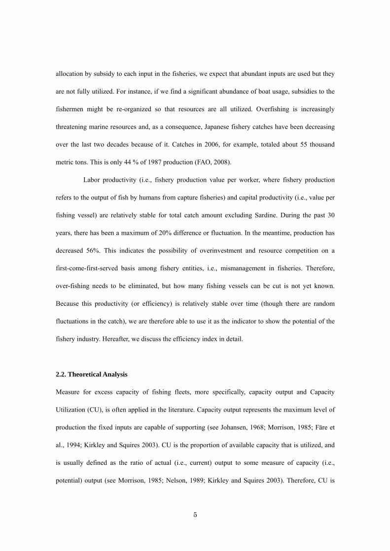
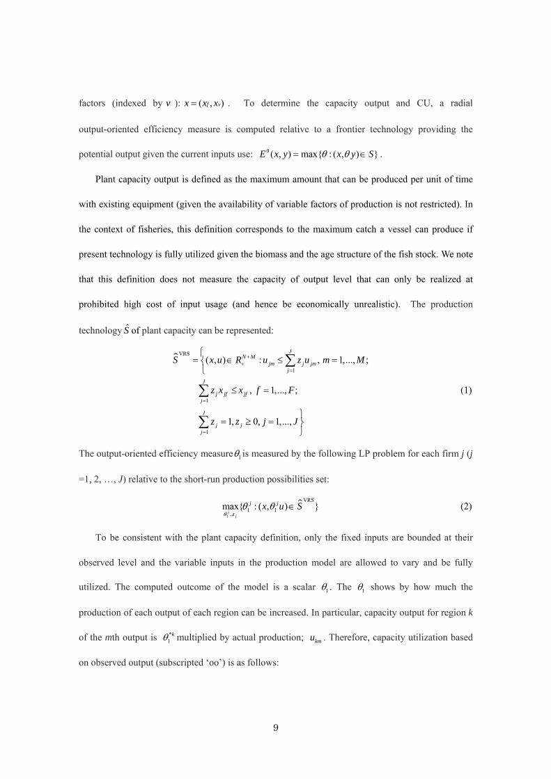
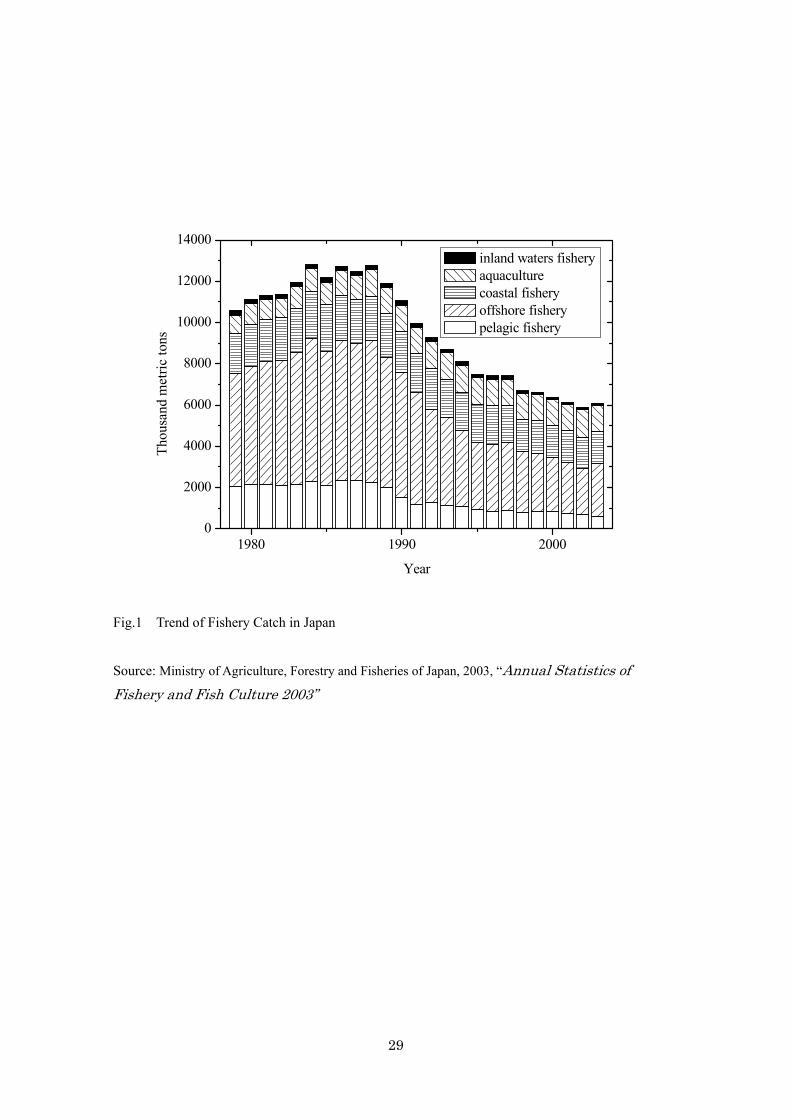
The fish catch in Japan has been decreasing drastically due to overfishing since 1989, even though it

had showed a continuous increase from the late 1970s (Figure 1). Given the declining fish catches,

1 The allocated shares are bought and sold like shares of stock in a company. Shareholders in the fishery are each guaranteed a percentage of the catch. The number of fish that each fisherman may catch is usually based on past averages. The catch share systems are already common in Australia, New Zealand and Iceland, while they have been gaining popularity in Canada and the United States. Though our model directly shows how much each individual needs to catch (and use as effort), we do not allow market mechanism in the model. In this sense, it is different from the catch shares concept. However, we are able to show optimal individual catch combinations, so that total catch is divided to each catch share.

4

the Japan Fisheries Agency enacted the “Basic Law on Fisheries Policy” in June 2001. The law is a

new guideline for fishery policy replacing the “Coastal Fishery and Others Promotion Law” of 1963,

whose primary aim was to improve fishery productivity. The Basic Law has two key concepts: 1)

securing a stable supply of fishery products; and 2) the sound development of the fisheries industry

to promote the appropriate conservation and management of marine living resources.

In 1995, the Japan Fisheries Agency started to reduce the number of fishing vessels and

restrictions on fishing area and/or period for some fisheries in order to ensure the sustainable use of

fishery resources. The Total Allowable Catch (TAC) system has also been implemented. The

principal laws are “The Fisheries Law”, the “Living Aquatic Resources Protection Law” and the

“Law Concerning Conservation and Management of Marine Living Resources.” These principal

laws were also amended in keeping with the concept of the “Basic Law on Fisheries Policy.” The

central and prefectural governments regulate fishing efforts in terms of fishing methods. The TAC

system assigns TAC allocations to each fishery separately, not to individual fishermen. While seven

fish species are subject to the TAC system, covering about 30% of total fishing in Japan in 2000,

Total Allowable Effort (TAE) was established as a system to manage total allowable effort with the

amendment of the “Law Concerning Conservation and Management of Marine Living Resources.”

The TAE includes curtailing the number of boats, suspension of operations, and improvement of

fishing gear among others. However, these regulations are not effective and the catch has been

decreasing continuously. Essentially, the regulations are too loose to control the actual activities of

fishermen.

For decades, the Fisheries Agency subsidized an expansion of its own national fleets,

leading to increased fishing in coastal regions for financial supports. Without subsidies, most

fishermen need to exit from the market. Therefore, our interest is in understanding production

performance in the disaggregated regional species level. Because of the distortion of resource

5

allocation by subsidy to each input in the fisheries, we expect that abundant inputs are used but they

are not fully utilized. For instance, if we find a significant abundance of boat usage, subsidies to the

fishermen might be re-organized so that resources are all utilized. Overfishing is increasingly

threatening marine resources and, as a consequence, Japanese fishery catches have been decreasing

over the last two decades because of it. Catches in 2006, for example, totaled about 55 thousand

metric tons. This is only 44 % of 1987 production (FAO, 2008).

Labor productivity (i.e., fishery production value per worker, where fishery production

refers to the output of fish by humans from capture fisheries) and capital productivity (i.e., value per

fishing vessel) are relatively stable for total catch amount excluding Sardine. During the past 30

years, there has been a maximum of 20% difference or fluctuation. In the meantime, production has

decreased 56%. This indicates the possibility of overinvestment and resource competition on a

first-come-first-served basis among fishery entities, i.e., mismanagement in fisheries. Therefore,

over-fishing needs to be eliminated, but how many fishing vessels can be cut is not yet known.

Because this productivity (or efficiency) is relatively stable over time (though there are random

fluctuations in the catch), we are therefore able to use it as the indicator to show the potential of the

fishery industry. Hereafter, we discuss the efficiency index in detail.

2.2. Theoretical Analysis

Measure for excess capacity of fishing fleets, more specifically, capacity output and Capacity

Utilization (CU), is often applied in the literature. Capacity output represents the maximum level of

production the fixed inputs are capable of supporting (see Johansen, 1968; Morrison, 1985; Färe et

al., 1994; Kirkley and Squires 2003). CU is the proportion of available capacity that is utilized, and

is usually defined as the ratio of actual (i.e., current) output to some measure of capacity (i.e.,

potential) output (see Morrison, 1985; Nelson, 1989; Kirkley and Squires 2003). Therefore, CU is

6

measured on a 0 to 1 scale. When CU is less than 1, one could produce more catch than current catch

if inputs are fully utilized. In other words, smaller inputs are enough (assuming they are fully

utilized) to produce same level of current catch. The purpose of this study is to measure the capacity

output and CU of Japan’s fisheries. Then, we examine how much cost reductions they can achieve in

a well-controlled world using unique disaggregated data covering all areas in Japan. If there is less

capacity output in Japan’s fisheries, there would be less reduction of fishing vessels and more

investment flexibility assuming potential fluctuations in the future. On the other hand, if there is

large capacity output, there should be an increased reduction of fishing vessels.

The more detailed purpose of this study is to find the optimal inputs/outputs mix of

Japanese fisheries. In this study, we apply the revised Johansen industry model to measure the

capacity outputs following Kesterns et al. (2006). This model consists of two steps of different linear

programming (LP) techniques. First, we measure the capacity output by using output-oriented DEA.

Second, we measure the optimal fixed inputs given in certain fishery quotas.

Optimal scales of outputs and fixed factor inputs indicate the required total outputs and

inputs at industry level. Calculated loss of efficiency shows the possible reduction of the fixed inputs.

The capacity outputs assume variable return to scale (VRS) in our model to be flexible. The

production frontier is calculated based on the maximum outputs given current inputs.

2.3. Literature Review

Recently, a sophisticated model of the multi-output/input frontier-based short-run Johansen

industry model has been developed by Kesterns et al. (2006). In the literature of fishery economics,

there are few studies on the capacity at the industry level other than Färe et al. (2001) and Kesterns

et al. (2006). In the industry model, capacities of individual fishery entities are utilized by

minimizing fixed industry inputs given their total outputs, capacities and the current state of

7

technology. We assume the variable inputs are allowed to vary and be fully utilized. Based on Färe

et al. (2001), Kesterns et al. (2006) sophisticated empirical models are developed to analyze capacity

outputs of the Danish fleets, extending to scenario analyses of tightening quota, seasonal closure

policies, lower and upper bounds, decommissioning schemes and area closures. The results show

that vessel numbers can be reduced by about 14 percent and the use of fixed inputs by around 15

percent, depending on the specific objective and policy mix in the Danish fishery.

We introduce three empirical studies using the Data Enveloped Analysis (DEA) to estimate

fishery CU. Niels et al. (2003) measure three types of CU applied to the Danish Gillnet fleet using

output-oriented DEA. As a result, the average CU of the Danish Gillnet fleet was found to be

between 0.85 and 0.95, and excess capacities for cod and sole are higher than for other species. The

result using the variable input utilization shows the output could have been increased on average by

27 percent in the period examined. Therefore, the numbers of fishing operations will be increased by

27 percent.

Many developing countries follow offshore fisheries development strategies (e.g., Kirkley

et al., 2003). This is to increase protein supply, expand employment, earn foreign exchange, and

mitigate the conflict between large- and small-scale fisheries over the inshore resource stocks. To

evaluate the successful fishery policies of the Peninsular Malaysian fishery, Kirkley et al. (2003)

analyze the west coast purse seine fishery in Malaysia to estimate the CU, and the crew utilization

among others. The results tell us the Malaysian fishery has a very high level of technical

efficiency.

Dupont et al. (2002) examine capacity and capacity utilization of the Nova Scotia mobile

gear fishery by using individual firm data before and after the implementation of Individual

Transferable Quotas (ITQs). The purpose of their study is examining how a change in the property

rights regime can affect a multi-product industry and the consequences in terms of product-specific

8

CU, as well as aggregate CU. The result provides insights for market based approaches to improve

efficiency in multi-product industries.

Among earlier studies applying DEA to the fishery industry to computing CU, there are

few empirical studies discussing how much the industry inputs could be reduced, other than Kesterns

et al. (2006). In addition, there are few studies evaluating Japanese fishery efficiency because the

fisheries are extensive and diversified and there may be difficulties obtaining Japanese fisheries data.

In this study, we focus on the efficiency of all Japanese fisheries, especially the reduction of the

fixed factor inputs.

3. Model

3.1. Industry Model

Following the revised short-run Johansen model of Kesterns et al. (2006), we compute marine

fishery efficiencies in Japan. The conceptual model proceeds in two steps. In the first step, the

capacity measure is compared to determine capacity production for each fishery entity at the

production frontier. The capacity production is calculated by output-oriented DEA model assuming

strong disposal of inputs and outputs, and variable returns to scale. In the second step, individual

entity capacities are utilized with the minimization of fixed industry inputs given total outputs,

capacities, and current state of technologies. This capacity measure is short-run because it does not

assume any change in the existing firm-level capacity, and it is a technical rather than an economic

capacity notion.

The following models are applied in this study. The production technology S transforms

inputs 1( ,..., ) nnx x x R+= ∈ into outputs 1( ,..., ) m

mu u u R+= ∈ and summarizes the set of all feasible

input and output vectors: {( , ) : can produce }n mS x u R x u++= ∈ . Let J be the number of regional

units. The n-dimensional input vector x is partitioned into fixed factors (indexed by f ) and variable

9

factors (indexed by v ): ( , )f vx x x= . To determine the capacity output and CU, a radial

output-oriented efficiency measure is computed relative to a frontier technology providing the

potential output given the current inputs use: 0 ( , ) max{ : ( , ) }E x y x y Sθ θ= ∈ .

Plant capacity output is defined as the maximum amount that can be produced per unit of time

with existing equipment (given the availability of variable factors of production is not restricted). In

the context of fisheries, this definition corresponds to the maximum catch a vessel can produce if

present technology is fully utilized given the biomass and the age structure of the fish stock. We note

that this definition does not measure the capacity of output level that can only be realized at

prohibited high cost of input usage (and hence be economically unrealistic). The production

technology S of plant capacity can be represented:

$VRS

1

1

1

( , ) : , 1,..., ;

, 1,..., ;

1, 0, 1,...,

JN M

jm j jmj

J

j jf jfj

J

j jj

S x u R u z u m M

z x x f F

z z j J

++

=

=

=

⎧= ∈ ≤ =⎨⎩

≤ =

⎫= ≥ = ⎬

⎭

∑

∑

∑

(1)

The output-oriented efficiency measure 1θ is measured by the following LP problem for each firm j (j

=1, 2, …, J) relative to the short-run production possibilities set:

$1

VRS

1 1,

max{ : ( , ) }j

j

j j

zx u S

θθ θ ∈ (2)

To be consistent with the plant capacity definition, only the fixed inputs are bounded at their

observed level and the variable inputs in the production model are allowed to vary and be fully

utilized. The computed outcome of the model is a scalar 1θ . The 1θ shows by how much the

production of each output of each region can be increased. In particular, capacity output for region k

of the mth output is *1

kθ multiplied by actual production; kmu . Therefore, capacity utilization based

on observed output (subscripted ‘oo’) is as follows:

10

oo *1

1CUkkθ

= (3)

This ray CU measure may be biased downward (see Färe et al., 1994). This is because there is

no guarantee the observed outputs are not produced in a technically efficient way. The problem of

technically efficient measure is solved given that both the variable and fixed inputs are constrained

to their current level. Another technical efficiency measure is obtained by evaluating each region j =

1, 2, ..., J relative to the production possibility set VRSS :

VRS

1

1 1

( , ) : , 1,..., ;

, 1,..., ; 1, 0, 1,...,

JN M

jm j jmj

J J

j jn jn j jj j

S x u R u z u m M

z x x n N z z j J

++

=

= =

⎧= ∈ ≤ =⎨⎩

⎫≤ = = ≥ = ⎬

⎭

∑

∑ ∑. (4)

The outcome ( 2θ ) shows by how much production can be increased using the technically efficient

inputs:

2

VRS2 1

,max{ : ( , ) }

jj

j j

zx u S

θθ θ ∈ (5)

The technically efficient output vector is 2θ multiplied by observed production for each output.

The technically efficient output (subscripted ‘eo’), or unbiased ray measure of capacity utilization, is

calculated as:

*2

eo *1

CUk

kk

θθ

= (6)

We focus on reallocating catches between vessels by explicitly allowing improvements in

technical efficiency and capacity utilization rates. The model is developed in two steps as follows.

An optimal activity vector *kz is provided for region k from model (1), and thus capacity output and

the optimal use of fixed and variable inputs are computed in the first step:

* * * * * * * *; ;k k k k kkm j jm jm kf j jf jf kv j jv

j j j

u z u s x z x s x z x= − = + =∑ ∑ ∑ (7)

where *kjms and *k

jfs are the optimal surplus and slack variables corresponding to the output,

respectively, fixed input dimensions.

11

In a second step, these ‘optimal’ frontier figures (i.e., capacity output and capacity variable and

fixed inputs) at regional level are used as parameters in the industry model. Particularly, the

industry model minimizes the industry use of fixed inputs in a radial way such that the total

production is at least the current total level (or at a quota level in the model extended later) by a

reallocation of production between regions. Reallocation is allowed based on the frontier production

and input usage of each region. In the short run, we assume that current capacities cannot be

exceeded either at the regional or industry level. Define Um as the industry output level of output m

and Xf (Xv) as the aggregate fixed (variable) inputs available to the sector of factor f (v), i.e.:

, ,m jm f fj v vjj j j

U u X x X x= = =∑ ∑ ∑ . (8)

The formulation of the multi-output and frontier-based industry model can then be specified as:

, ,

*

*

*

min

s.t. , 1,..., ,

, 1,..., ,

0, 1,..., ,

0 1, 0, 1,..., .

vw X

jm j mj

fj j fj

v vj jj

j

u w U m M

x w X f F

X x w v V

w j J

θθ

θ

θ

≥ =

≤ =

− + ≤ =

≤ ≤ ≥ =

∑

∑

∑

(9)

3.2. Extension of Industry Model

We turn to the second-stage industry model (9). First, following the second modification above,

the constraints for each output dimension have to reflect the fact that production may take place in

different areas. That is, there are M output constraints (species) for each of the A areas:

* , 1,..., , 1,...,jma ja maj

u w U m M a A≥ = =∑ . (10)

Each region j has one area a because the area corresponds to the place each aggregated entity

belongs. Second, the industry consists of fishery entities or vessels fishing in different areas. The

constraints for each of the total fixed inputs can be formulated in a most general way in terms of

12

constraints indexed by area:

*

,

, 1,...,fja ja fj a

x w X f Fθ≤ =∑ (11)

Third, the constraints on the variable inputs are:

*

,

0, 1,...,v vja jaj a

X x w v V− + ≤ =∑ (12)

To offer a menu of current and potential conservation and distributional policies in fisheries, we

add some further refinements to the short-run industry model of Dervaux et al. (2000). We here

focus on four issues: (i) seasonal closures, putting limits on fishing days, (ii) partial tolerance of

technical inefficiencies, (iii) the link between economic and plant capacity, and (iv) tightening quotas

of either species.

(i) Seasonal closure policies limit the number of fishing days in an effort to control inputs. To

limit the amount of variable inputs that appear in the model as an aggregate decision variable, we fix

a constraint on the total annual fishing days at FDmax common to all business entities. This can be

simply represented as follows:

*maxFD , 1vja ja

ax w v≤ =∑ (13)

given that the fishing days are indexed by v equal to 1 (i.e. the first variable input). In this study,

FDmax is 200 for all the entities when seasonal closure is imposed, and otherwise is 365 as

unconstrained parameter.

(ii) The frontier nature of the underlying technologies may push things too far so that it is

practically impossible to require vessels to adjust immediately to technically efficient production

plans. While technical efficiency is a condition for any social optimum, realistic planning

procedures may require tolerating technical inefficiency for part of this path for informational and

political reasons (Peters, 1985).

This can be modeled by adjusting the capacity output, which enter to the second stage industry

13

model, by its current observed technical inefficiency and ultimately corrected by an efficiency

improvement imperative (α ) (see Kesterns el al., 2006). Of course, technically efficient regions at

present need no such adjustment. Therefore, assuming this correction factor is smaller or equal to

unity ( 1α = ), adjustment of the second stage capacity output could take the following form when

technical inefficiency is (partially) accepted:

**

*1

ˆ0,max{1, }

1,..., , 1,...,

jmajma

uu

j J a A

θαθ

≥ =

= =

(14)

In this research α is 0.1 for all the entities when technical inefficiencies are tolerated partially.

When α is set to be 0.1, capacity outputs of all the entities is limited up to 10 times of current

output.

(iii) Lower bounds (LB) and upper bounds (UB) are introduced on the activity vectors to avoid

economically unviable solutions (i.e., LB) and production at technical capacity levels that are

beyond economic capacity levels (i.e., UB), respectively. This indirectly includes economic

information into an otherwise technical production model.

LB UB, 1,..., , 1,...,jaw j J a A≤ ≤ = = (15)

In this research LB is 0 or 0.1 and UB is 1 or 0.9 as unconstrained and constrained parameters,

respectively.

(iv) We consider setting quotas such as TAC for particular species in Japan. We simply add the

constraint:

, 1, 0 1ma m m ma

U U Q m Q= ⋅ = ≤ ≤∑ (16)

given that the species are indexed by m equal to 1 (i.e. the first output). mQ indicates a quota rate

for the mth current industry output. In this study mQ is incremented by 0.01 from 0 to 1 for

sensitivity analysis purpose.

We sum up the above mentioned constraints and our model is shown as follows:

14

, ,

*

*

,

*

,

*max

**

*1

min

ˆs.t. , 1,..., , 1,...,

, 1,...,

0, 1,...,

LB UB,

, 1

FD , 1

ˆ0,max{1, }

1,..., , 1,..., , 0 1

vw X

jma ja maj

fj ja fj a

v vj jaj a

ja

ma m ma

vja jaa

jmajma

m

u w U m M a A

x w X f F

X x w v V

w

U U Q m

x w v

uu

j J a A Q

θθ

θ

θαθ

≥ = =

≤ =

− + ≤ =

≤ ≤

= ⋅ =

≤ =

≥ =

= = ≤ ≤

∑

∑

∑

∑

∑

(17)

4. Data and Scenarios

4.1. Data

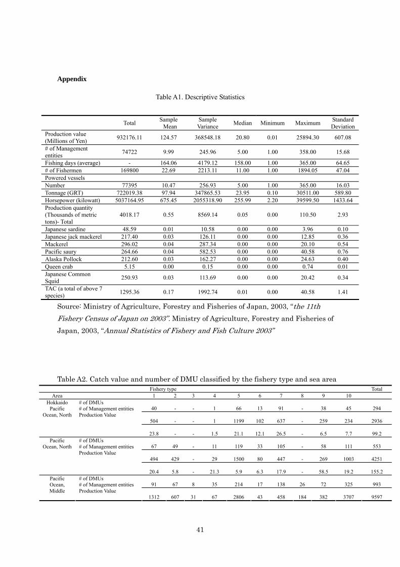
Data used in this study comes from the 11th Fishery Census of Japan on 2003 and Annual

Statistics of Fishery and Fish Culture 2003 by Ministry of Agriculture, Forestry and Fisheries of

Japan. The data set is composed of each aggregated fishery entity per municipality per marine

fishery type in Japan. The 2003 Fishery Census of Japan was conducted to clarify the structures of

fishery production in Japan, and to comprehend the overall background of fisheries concerning

fishing villages, marketing and processing industries among others. The purpose is developing basic

data for fisheries policies including improvements in the structure of fisheries.

Our output data is production value (in the unit of Japanese yen) and quantities data. There are

nine types of outputs used in this study, including total production quantity, all fishes, the other

marine animals, Japanese sardine, Japanese jack mackerel, Mackerel Pacific saury, Alaska Pollock,

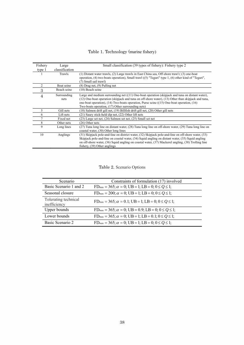
Queen crab, and Japanese Common Squid (Table 1). The TAC system in Japan applies to all these

seven species. For example, the Squid showed a slight decline although it still remains in a dominant

position. The Pollock has been on the decline mainly due to the subsequent fall of catch in the

15

Bering high seas. Mackerel have also decreased drastically over the years.

There are two variable inputs - labor and fishing days - and two fixed inputs of gross registered -

tons (Grt) and horse power (kilowatt) - for aggregated fishery entities of each municipality and

marine fishery type in Japan. The fixed inputs are both multiplied by the number of fishing days,

following Kesterns et al. (2006). The variable inputs are numbers of workers on board at peak times

and average fishing days of each aggregated entity. Descriptive statistics for each area are reported in

Table A1 in the Appendix. These data cover effectively all the Japanese fishery entities. The

aggregated fishery entities with missing values and fishing within 30 days are excluded in the

sample. In total, 74,728 fishery entities are covered in the data set of 7,483 observations. On average,

each aggregated fishery entity consists of about 10 entities (Table 1). We have 39 classifications of

marine fisheries in analyses. Basic allocation of fishery in each are, technology type, and fishery

species are provided in Table A2-A4 in the Appendix. Small whaling, diving apparatus fisheries,

shellfish collecting, seafood collecting, and other fisheries are excluded because we consider these

fisheries atypical cases.

We assume management decisions are provided in the disaggregated regional level, especially

models (1) and (4), because their decision making is applied to one given area and one given fishery

type. Thus, the efficiency of each aggregated fishery entity is evaluated relative to one of the

potentially 361 different technologies (nine areas by thirty-nine marine fishery types). The

technologies, which consist of only a few similar observations, may lead to biases in the estimation

of plant capacity due to a lack of comparable production units. To avoid downward estimation, we

use 10 large classifications and refer to the 10 and 39 fishery classifications as fishery type 1 and 2,

respectively (see Table 1). Therefore, there are potentially 90 and 361 different technologies in

fishery type 1 and 2. We use mainly fishery type 1, and compare type 1 with type 2 in an

unconstrained scenario.

16

4.2. Scenarios

In each specification, we apply several different types of output variables. In the first two

specifications, production value and production quantity are used as the output variables,

respectively, and we compare both efficiencies. Second, we divide the estimated production quantity

into two and three categories, which are (a) TAC species and the others including (b) fish and (c) the

other marine animals. The aim of this division is to set production quotas only for respective TAC

species, and to compare the efficiencies of each group.

We classify a series of scenarios, systematically testing the effect of additional constraints. The

results of several policy-oriented scenarios with various constraints are useful for policy implications.

These scenarios are summarized in Table 2. Basic scenario 1 is the basic industry model without

any particular constraints. The seasonal closure scenario limits the number of average fishing days to

200 each year. The tolerated technical inefficiencies scenario allows for technical inefficiencies, but

already imposes an improvement imperative of 1000 per cent (thus, α = 0.1). The UB scenario looks

at the impact of UB on the activity or intensity vector, and the UB is fixed at 0.9. The LB scenario as

well as the UB scenario look at the impact of LB, and the LB was set equal to 0.1. These five

scenarios use fishery type 1. Basic scenario 2 uses fishery type 2 without any particular constraints.

We compute the optimal inputs in the industry model. We follow Kesterns et al. (2006) to set the

optimal fixed inputs (Grt and kw) and variable inputs (labor and fishing days) as * * */ ( )f vX w Xθ ⋅

and * *vw X⋅ , respectively. We also estimate optimal fishery expenditures (such as wage, vessels,

implements, and oil) to understand how much expenditures could be reduced in a reallocated world.

We calculate them using average expenditure percentages of total fishery income among fishery

business entities from 1961 to 2000. The reason why we only refer to the expenditures of business

entities is that labor costs of fishery households are difficult to interpret because the costs are

17

considered to be included in their discretionary incomes. On average, wages, vessels, implements,

and oil account for 36.5%, 7.2%, 3.9%, and 11.6% of total fishery income during the period,

respectively (Table A5 )2.

5. Empirical Results

5.1. Scenario Analyses

(a) Current and Capacity Outputs

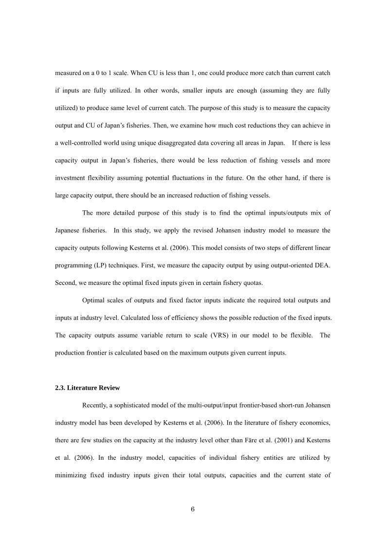
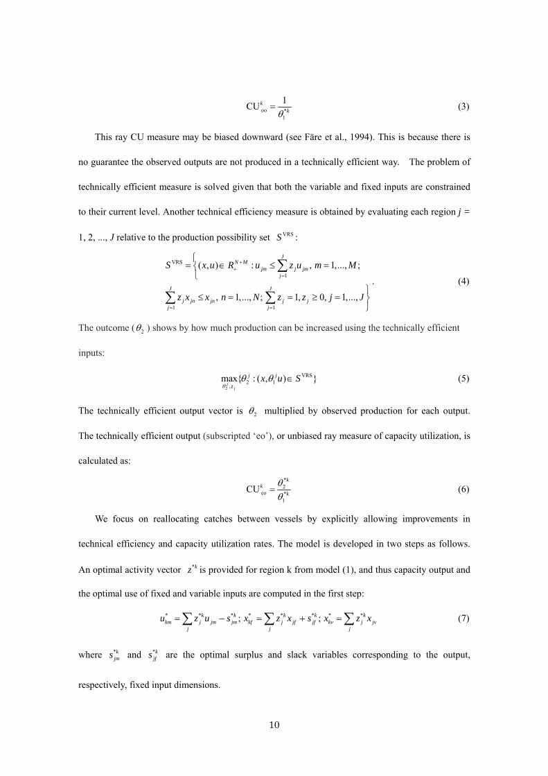
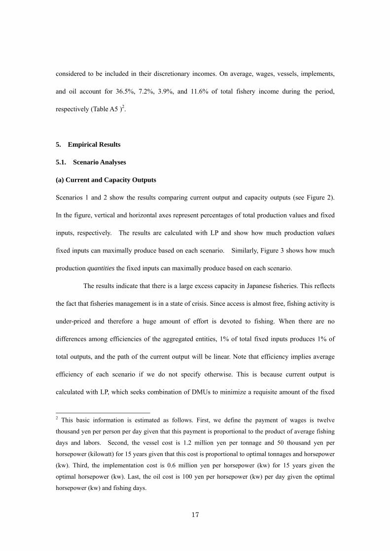
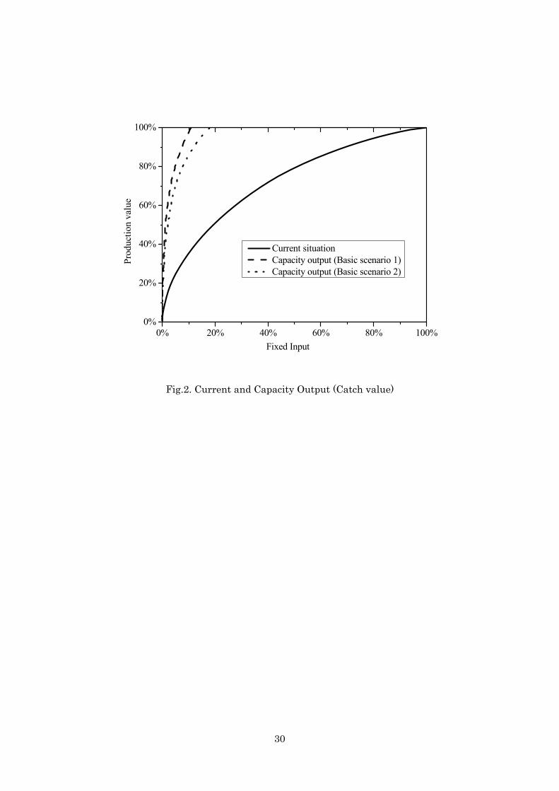
Scenarios 1 and 2 show the results comparing current output and capacity outputs (see Figure 2).

In the figure, vertical and horizontal axes represent percentages of total production values and fixed

inputs, respectively. The results are calculated with LP and show how much production values

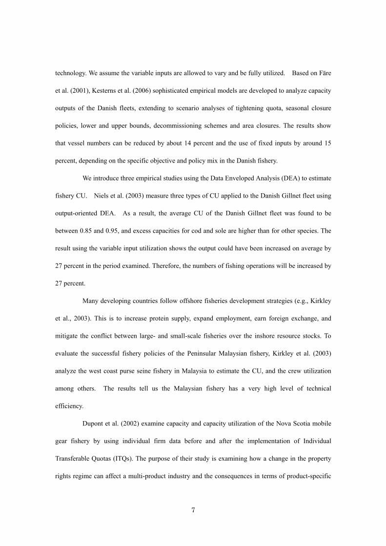
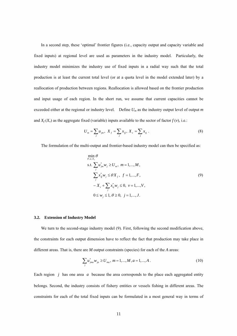
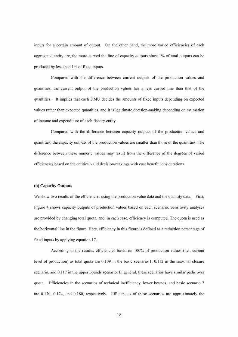
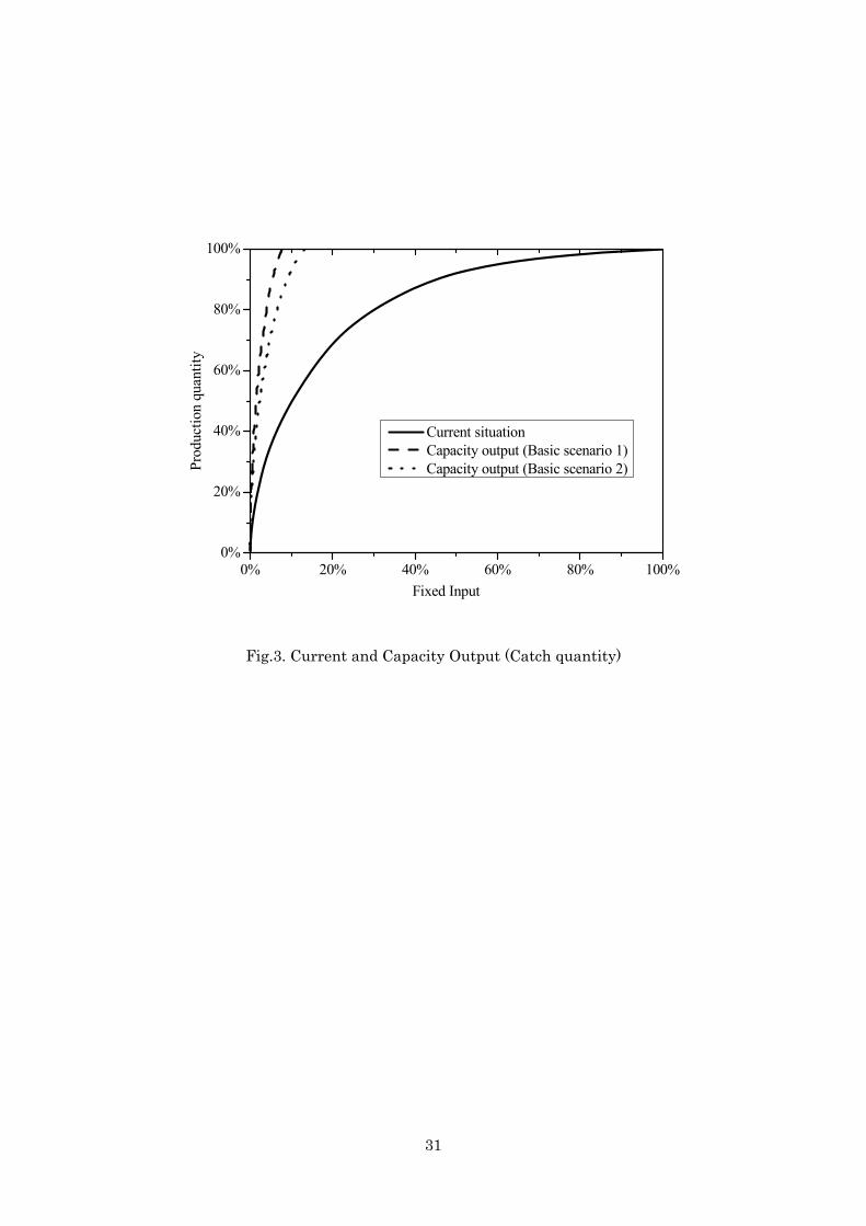
fixed inputs can maximally produce based on each scenario. Similarly, Figure 3 shows how much

production quantities the fixed inputs can maximally produce based on each scenario.

The results indicate that there is a large excess capacity in Japanese fisheries. This reflects

the fact that fisheries management is in a state of crisis. Since access is almost free, fishing activity is

under-priced and therefore a huge amount of effort is devoted to fishing. When there are no

differences among efficiencies of the aggregated entities, 1% of total fixed inputs produces 1% of

total outputs, and the path of the current output will be linear. Note that efficiency implies average

efficiency of each scenario if we do not specify otherwise. This is because current output is

calculated with LP, which seeks combination of DMUs to minimize a requisite amount of the fixed

2 This basic information is estimated as follows. First, we define the payment of wages is twelve

thousand yen per person per day given that this payment is proportional to the product of average fishing

days and labors. Second, the vessel cost is 1.2 million yen per tonnage and 50 thousand yen per

horsepower (kilowatt) for 15 years given that this cost is proportional to optimal tonnages and horsepower

(kw). Third, the implementation cost is 0.6 million yen per horsepower (kw) for 15 years given the

optimal horsepower (kw). Last, the oil cost is 100 yen per horsepower (kw) per day given the optimal

horsepower (kw) and fishing days.

18

inputs for a certain amount of output. On the other hand, the more varied efficiencies of each

aggregated entity are, the more curved the line of capacity outputs since 1% of total outputs can be

produced by less than 1% of fixed inputs.

Compared with the difference between current outputs of the production values and

quantities, the current output of the production values has a less curved line than that of the

quantities. It implies that each DMU decides the amounts of fixed inputs depending on expected

values rather than expected quantities, and it is legitimate decision-making depending on estimation

of income and expenditure of each fishery entity.

Compared with the difference between capacity outputs of the production values and

quantities, the capacity outputs of the production values are smaller than those of the quantities. The

difference between these numeric values may result from the difference of the degrees of varied

efficiencies based on the entities' valid decision-makings with cost benefit considerations.

(b) Capacity Outputs

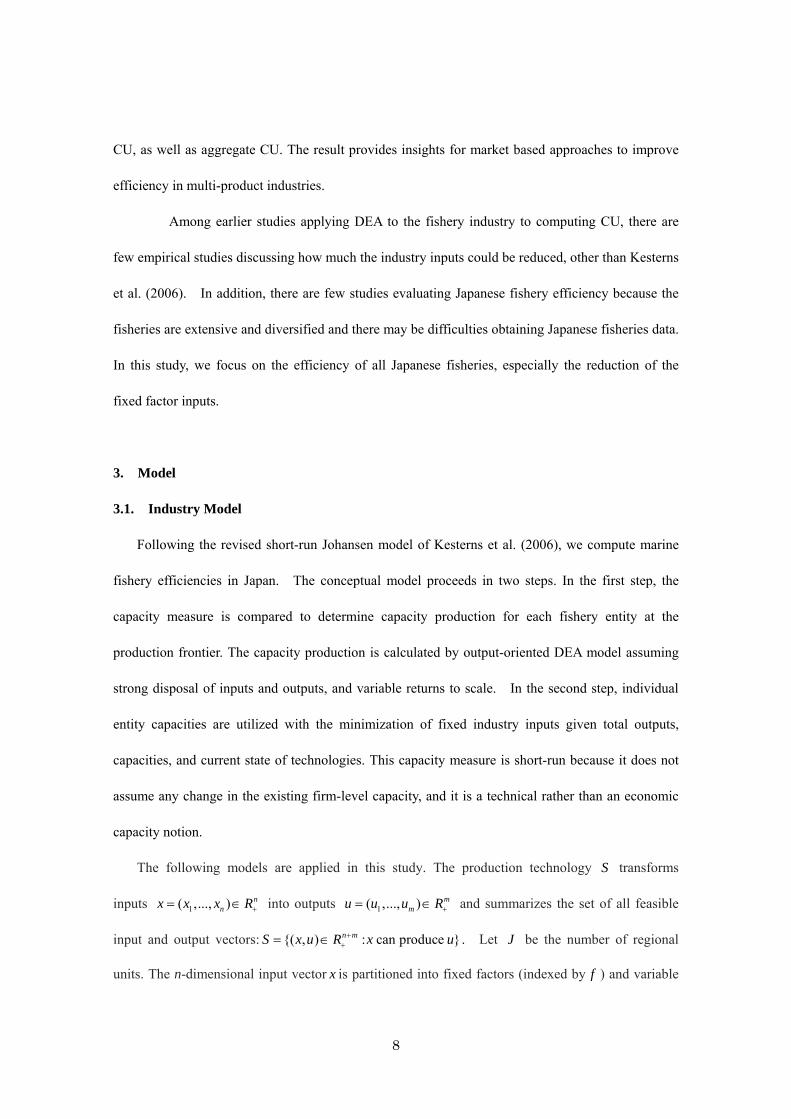
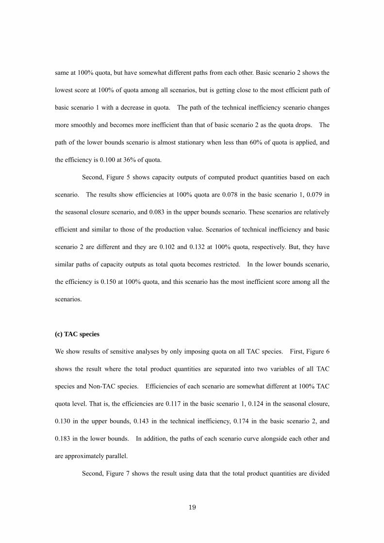
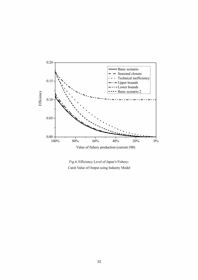
We show two results of the efficiencies using the production value data and the quantity data. First,

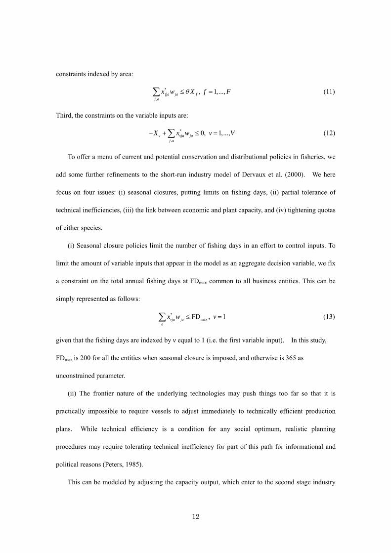
Figure 4 shows capacity outputs of production values based on each scenario. Sensitivity analyses

are provided by changing total quota, and, in each case, efficiency is computed. The quota is used as

the horizontal line in the figure. Here, efficiency in this figure is defined as a reduction percentage of

fixed inputs by applying equation 17.

According to the results, efficiencies based on 100% of production values (i.e., current

level of production) as total quota are 0.109 in the basic scenario 1, 0.112 in the seasonal closure

scenario, and 0.117 in the upper bounds scenario. In general, these scenarios have similar paths over

quota. Efficiencies in the scenarios of technical inefficiency, lower bounds, and basic scenario 2

are 0.170, 0.174, and 0.180, respectively. Efficiencies of these scenarios are approximately the

19

same at 100% quota, but have somewhat different paths from each other. Basic scenario 2 shows the

lowest score at 100% of quota among all scenarios, but is getting close to the most efficient path of

basic scenario 1 with a decrease in quota. The path of the technical inefficiency scenario changes

more smoothly and becomes more inefficient than that of basic scenario 2 as the quota drops. The

path of the lower bounds scenario is almost stationary when less than 60% of quota is applied, and

the efficiency is 0.100 at 36% of quota.

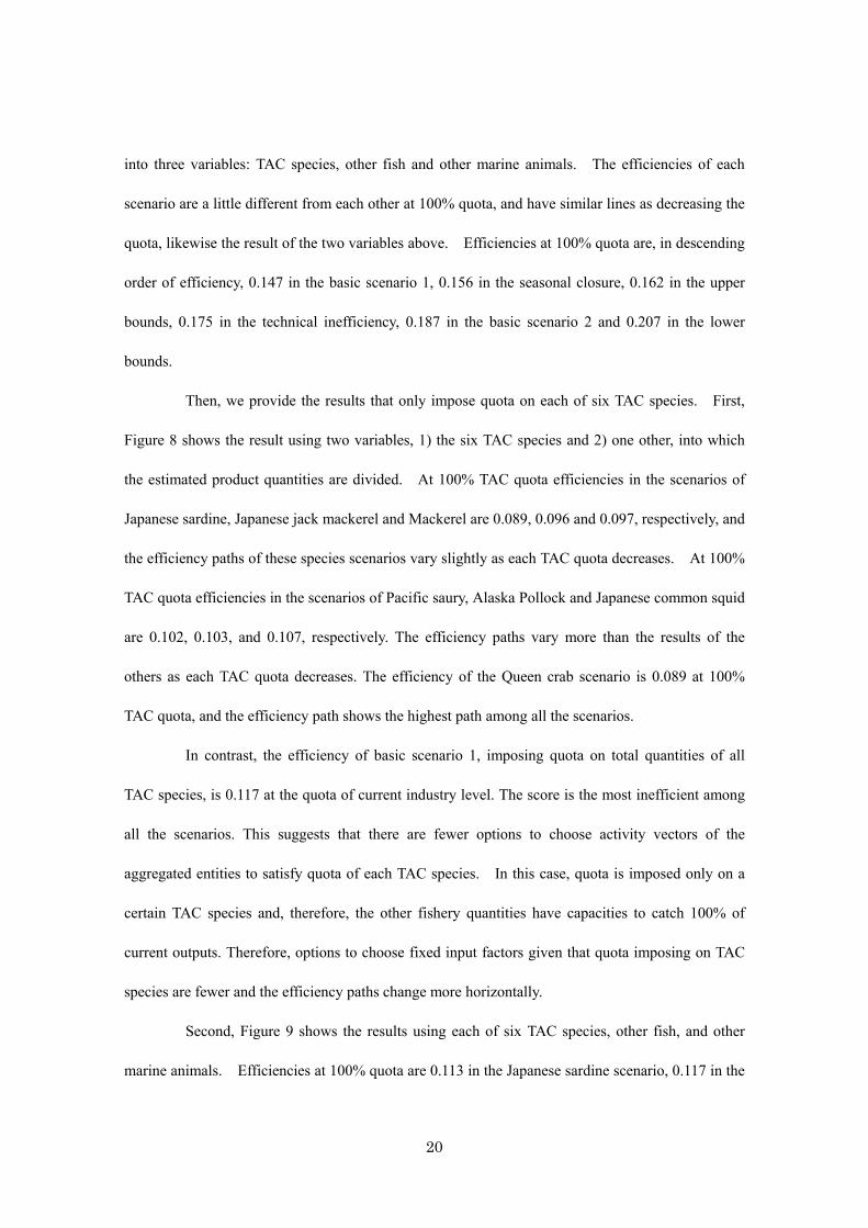
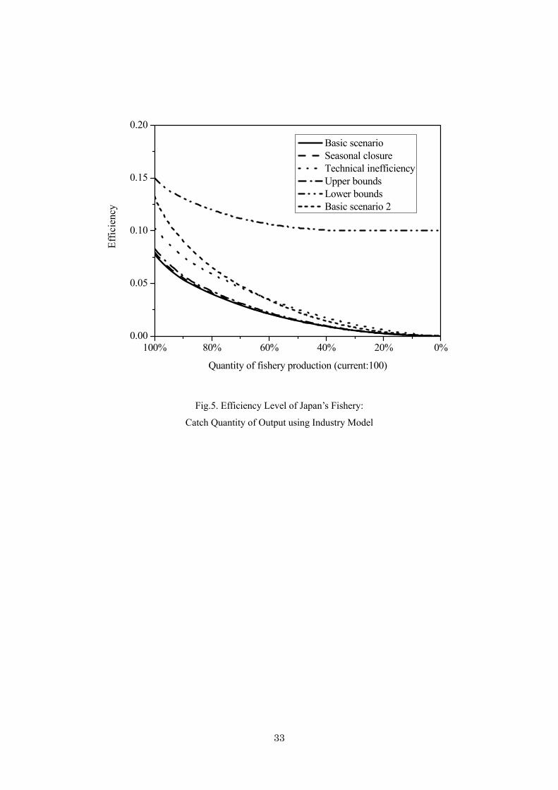
Second, Figure 5 shows capacity outputs of computed product quantities based on each

scenario. The results show efficiencies at 100% quota are 0.078 in the basic scenario 1, 0.079 in

the seasonal closure scenario, and 0.083 in the upper bounds scenario. These scenarios are relatively

efficient and similar to those of the production value. Scenarios of technical inefficiency and basic

scenario 2 are different and they are 0.102 and 0.132 at 100% quota, respectively. But, they have

similar paths of capacity outputs as total quota becomes restricted. In the lower bounds scenario,

the efficiency is 0.150 at 100% quota, and this scenario has the most inefficient score among all the

scenarios.

(c) TAC species

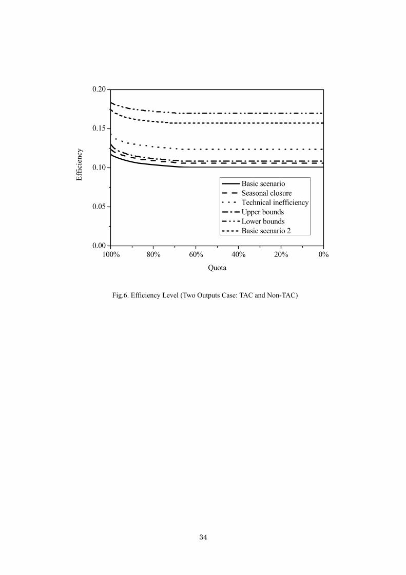
We show results of sensitive analyses by only imposing quota on all TAC species. First, Figure 6

shows the result where the total product quantities are separated into two variables of all TAC

species and Non-TAC species. Efficiencies of each scenario are somewhat different at 100% TAC

quota level. That is, the efficiencies are 0.117 in the basic scenario 1, 0.124 in the seasonal closure,

0.130 in the upper bounds, 0.143 in the technical inefficiency, 0.174 in the basic scenario 2, and

0.183 in the lower bounds. In addition, the paths of each scenario curve alongside each other and

are approximately parallel.

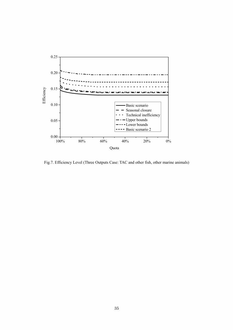
Second, Figure 7 shows the result using data that the total product quantities are divided

20

into three variables: TAC species, other fish and other marine animals. The efficiencies of each

scenario are a little different from each other at 100% quota, and have similar lines as decreasing the

quota, likewise the result of the two variables above. Efficiencies at 100% quota are, in descending

order of efficiency, 0.147 in the basic scenario 1, 0.156 in the seasonal closure, 0.162 in the upper

bounds, 0.175 in the technical inefficiency, 0.187 in the basic scenario 2 and 0.207 in the lower

bounds.

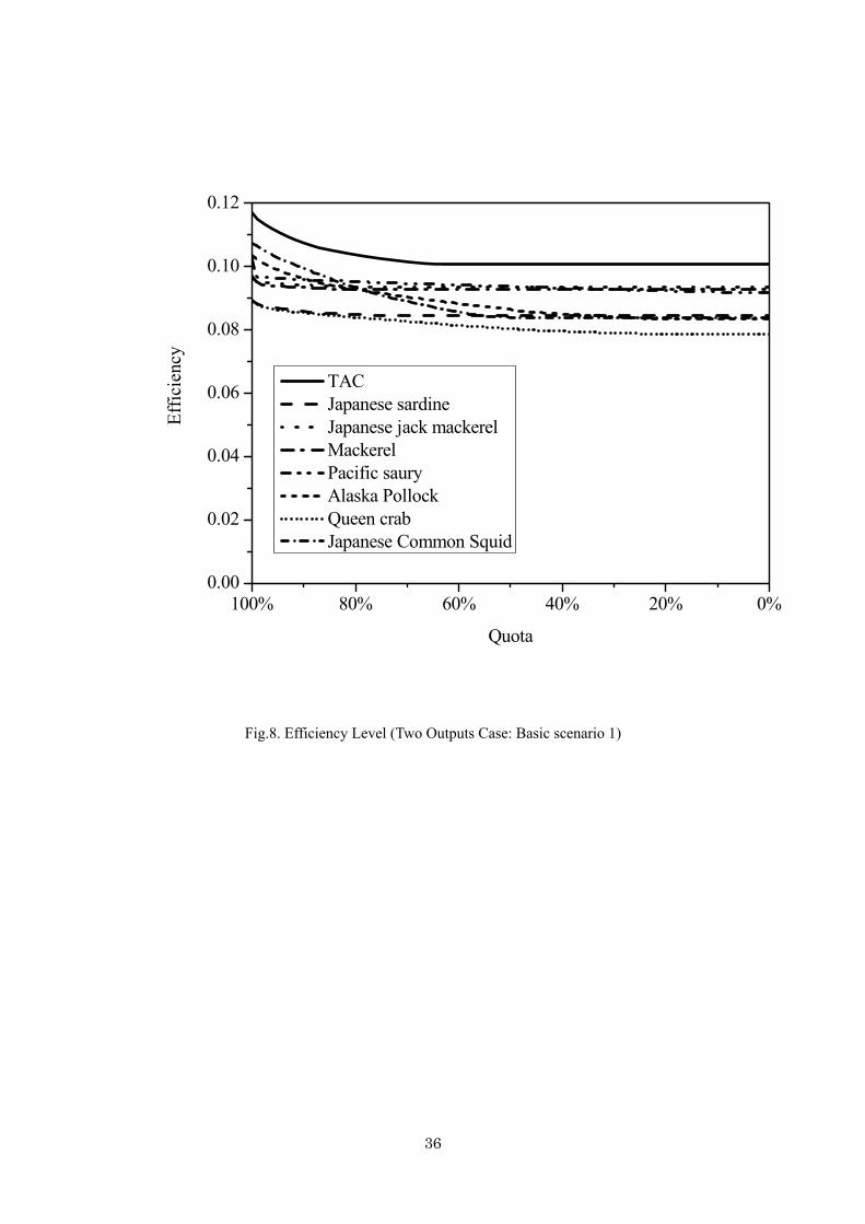
Then, we provide the results that only impose quota on each of six TAC species. First,

Figure 8 shows the result using two variables, 1) the six TAC species and 2) one other, into which

the estimated product quantities are divided. At 100% TAC quota efficiencies in the scenarios of

Japanese sardine, Japanese jack mackerel and Mackerel are 0.089, 0.096 and 0.097, respectively, and

the efficiency paths of these species scenarios vary slightly as each TAC quota decreases. At 100%

TAC quota efficiencies in the scenarios of Pacific saury, Alaska Pollock and Japanese common squid

are 0.102, 0.103, and 0.107, respectively. The efficiency paths vary more than the results of the

others as each TAC quota decreases. The efficiency of the Queen crab scenario is 0.089 at 100%

TAC quota, and the efficiency path shows the highest path among all the scenarios.

In contrast, the efficiency of basic scenario 1, imposing quota on total quantities of all

TAC species, is 0.117 at the quota of current industry level. The score is the most inefficient among

all the scenarios. This suggests that there are fewer options to choose activity vectors of the

aggregated entities to satisfy quota of each TAC species. In this case, quota is imposed only on a

certain TAC species and, therefore, the other fishery quantities have capacities to catch 100% of

current outputs. Therefore, options to choose fixed input factors given that quota imposing on TAC

species are fewer and the efficiency paths change more horizontally.

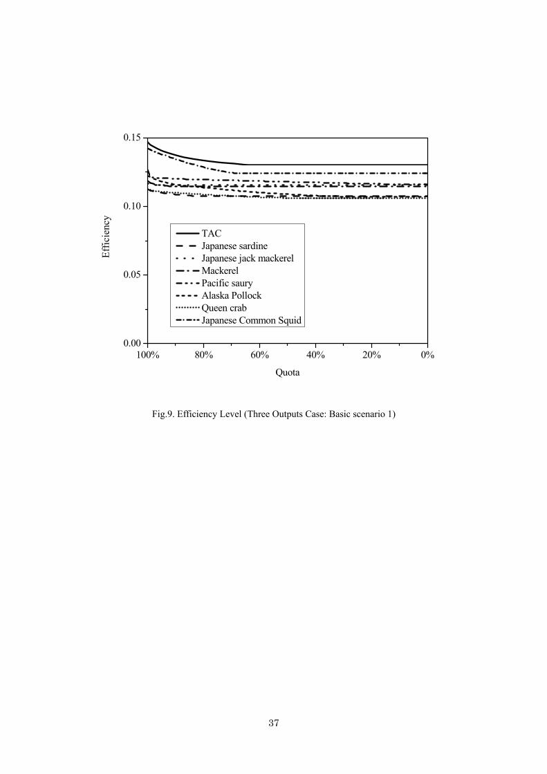
Second, Figure 9 shows the results using each of six TAC species, other fish, and other

marine animals. Efficiencies at 100% quota are 0.113 in the Japanese sardine scenario, 0.117 in the

21

Japanese jack mackerel scenario, 0.119 in the Mackerel scenario, 0.127 in the Pacific saury scenario,

0.122 in the Alaska Pollock scenario, 0.113 in the Queen crab scenario, 0.147 in the Japanese

common squid scenario, and 0.147 in the all TAC species scenario. The efficiency paths of the

Japanese Sardine and Queen crab scenarios are the most inefficient paths, and that of the all TAC

species scenario is the most inefficient, likewise the path using two variables above. The scenarios

of each TAC species, except Mackerel and Alaska Pollock, are nearly parallel to the horizontal line

at less than 95% of each quota. The scenarios of Mackerel and Alaska are nearly parallel at less than

70% and 50% quotas, respectively.

These varied efficiencies depend on the selection of outputs. When each output in each

category is separated in different model, the efficiency score will become even lower. It is difficult

to measure the efficiencies of each fishery method because there are many fishery species in the

Japanese sea and many fishery methods developed in the same regions. While we can estimate

efficiencies in various detailed cases using more disaggregated categories, it will become difficult to

discuss entire fisheries in Japan. The opposite is also true. Based on the results, the efficiency paths

are approximately the same among the cases, which vary only in quotas of each TAC species.

In summary, ensuring the current capacity outputs, except of certain TAC species, the fixed

inputs can satisfy the capacity outputs for the TAC species. Regarding the capacity outputs per

fishery area, the most efficient areas are the Japan Sea in the north of basic scenario 1 and the Pacific

Ocean in the south of basic scenario 2 (see Table A6 in Appendix). Most areas have excess

capacities of more than 100% in basic scenario 2. This implies that there are fixed inputs, which can

produce more than twice of the current quantities in Japan.

The most efficient fishery, where we define fish with the lowest excess capacity, is Pacific

Saury. There are excess capacities of 48.0% and 47.8% on Pacific Saury using the two and three

variables divided above (fishery type 1). The most inefficient fishery is for Japanese common

22

squid. There are excess capacities of 199.1% and 193.0%.

5.2. Reducing the Number of Fishery Entities

We compute the amount of non-zero activity vectors from the results above and provide the optimal

numbers of the aggregated fishery entities per Japanese sea area (Table A7 in Appendix). Among

all the scenarios, except the lower bounds scenarios, the optimal total number of fishery entities,

using the quantities data of 7,483 entities in our sample, are as follows; 1). 1,257 at a minimum in

the technically tolerated inefficiency scenario using one variable output, 2). 2,650 at a maximum in

the upper bounds scenario using the three variable outputs.

On average the optimal total DMU numbers are about 2,000. The values of the activity

vectors are almost at upper limits among all the scenarios (i.e., all inputs are utilized). One exception

is that the total of the lower bounds scenario is 7,483. We compute the numbers of fishery entities

by multiplying the active vector values and the numbers of entities in each aggregated entity level.

The minimum number is 5,704 in the basic scenario 1. Here we use the quantities data of two

variable outputs - Japanese sardine and other. The maximum number is 18,998 in the lower bounds

scenario using the production value data of one variable output.

We notice there are large differences among the optimal sizes of fishery entities in each

scenario. On average, however, the optimal size of the current Japanese fisheries is about one third

of current size. In other words, one third of the current fishery entities are required even if the central

government implements fishery policies in the most efficient way.

5.3. The Optimal Input Levels

We compute the optimal amounts of inputs in each scenario (see Table A8 in Appendix for detail).

These values are computed in the same manner as in section 4 to interpret the fixed inputs easily.

23

First, in the basic scenario 1 and 2, optimal input values of gross registered tons and horse powers

(kilowatt) are significantly smaller than optimal total fixed inputs as flow variables. In the basic

scenario 1 using the production value data, the optimal aggregated size is 10.85% of the current

fixed inputs. In the disaggregated data, these are 98.84% of the current average fishing days on

board, 1.76% of the current gross registered tons, and 1.51% of the horse powers.

In the seasonal closure scenarios, the optimal average fishing days are smaller than those

in the basic scenarios. However, the gross registered tons and horse powers are larger than those in

the basic scenarios. Using the production value data, the optimal sizes are 10.85% of the current

fixed inputs in the aggregate level. The disaggregated result shows these are 98.84% of the current

average fishing days, 1.76% of the current gross registered tons, and 1.51% of the horse powers.

Therefore, it is effective to reduce the fixed factor inputs rather than the fishing days. The fishery

entities enlarge the fixed inputs to deal with the seasonal closure. This shows that seasonal closure

policies may not contribute to capacity reduction.

In the technical inefficiency scenarios, the four inputs (of gross registered tons, horse

powers, optimal fishing days and labor power) are used more than in the basic scenario 1. In these

scenarios using the production value data, the optimal sizes are 17.00% of the current fixed inputs,

and the disaggregated results show values of 105.34% of the current average fishing days, 3.73% of

the current gross registered tons, and 3.27% of the horse powers. The optimal average fishing days

are average values of DMUs with non zero activity vectors and, therefore, more than 100% of the

average fishing days are in attendance on average.

In the upper bounds scenarios, results are similar to the seasonal closure scenarios. That is,

while the optimal average fishing days are smaller than those in the basic scenarios, the gross

registered tons and horse powers are larger than those in the basic scenarios. These imply that

when 10% of the aggregated entities’ activities are constrained, the aggregated entities will fish on

24

the upper limit days and enlarge the fixed inputs compared with the basic scenario 1.

Going through the amounts of the optimal inputs in each fishery type, we see that

allocating the fishery types in the most efficient way is different over specific fishery types (see

Table A9 in Appendix). In addition, a fishery type with a large amount of optimal inputs may not

be an efficient method itself, but a method with large capacity outputs from optimal inputs based on

the first step revised industry model. Relatively large amounts are types of surrounding nets (4),

Lift nets (6), Fixed nets (7) among others, and Long lines (9) especially are utilized little.

5.4. Estimates of Cost Reduction

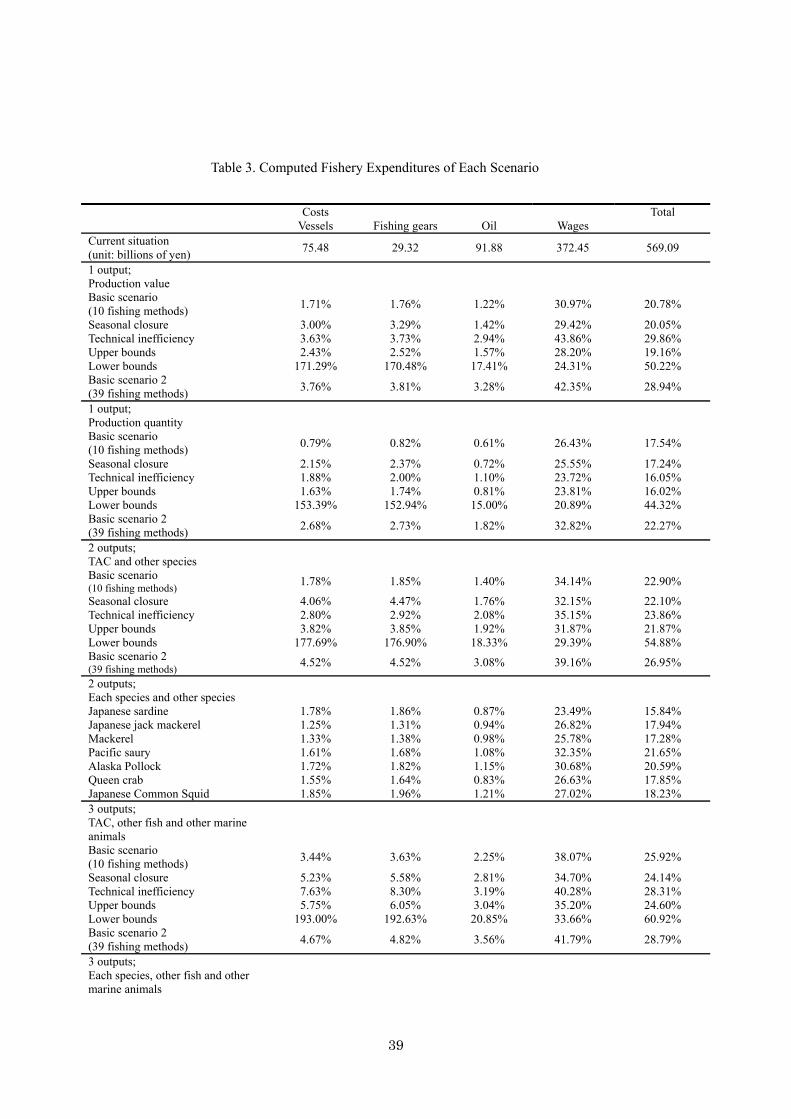
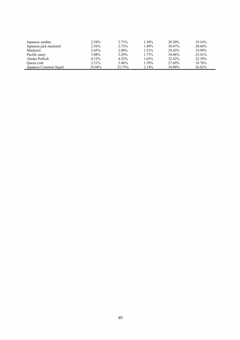
We compute the fishery expenditures of each scenario in Table 3. Overall, required costs of vessels,

fishing gears and oils (in our computed cases) are less than about 5 percent of current costs, and the

wages and total costs are about 30 and 20 percent, respectively, except the lower bounds scenarios.

In the basic scenario 1, using one output variable of the production value, what we need as costs of

vessels, fishing gears, oil, wages and total are 1.71%, 1.76%, 1.22%, 30.97%, and 20.78%,

respectively. The reduction in total number of fishing vessels represents a large amount of

reduction in total cost in the long run. These significant potential results are important for policy

purpose.

In the lower bounds scenarios, the optimal costs of vessel, fishing gears and oils are more

than 100% of the current costs. In addition, costs of oil, wages and total are about 15%, 20% and

50% of current costs, respectively. The total fishery expenditures in the seasonal closure scenarios

and the upper bounds scenarios are smaller than in the basic scenarios. This is because the necessary

average fishing days and labor powers in the two scenarios are fewer than those in the basic

scenarios 1.

25

6. Discussion and Conclusion

Global harvest peaked in about 1990 with the expansion of the fisheries to new regions.

Because there were no frontiers left to exploit, however, it declined after that (Andrew et al., 2002).

Macinko and Bromley (2002) argue the ITQ system is not a sufficient policy instrument to prevent

overfishing, instead providing individually specific catch shares of the TAC to each fisherman is the

key to avoid the race for fish. Thus, moving idea into practice with actual implementation of catch

shares, it is crucial to estimate the potential of cost reduction in the fishery industry assuming ideal

individually specific catch shares of the TAC is possible. This study analyzes the potential

calculation when a country decides to curb overfishing in the industry.

In Japan, the maximum level of production the fixed inputs are capable of supporting (i.e.,

capacity output) could be more than three times larger. Additionally, current overall fixed inputs

could be reduced to one-tenth. Furthermore, central government plans could reduce to one-third

fishery entities maintaining the capacity output to ensure the total fishery catch. Getting rid of these

inefficient fishers would help lead to sustainable fishery management. Furthermore, a

government-backed industry development program would need this type of change.

If the community can invest in adaptive governance of this allocation, we may move

toward a more sustainable path. The major weakness in our analysis is the assumption that marine

resources are fixed in the data we have. Of course, the resource stock changes over time and,

therefore, the computed outcome would be changed. We do not claim our computed inputs should

remain the same over time. Instead, this study urges that policy makers adopt a learning process by

suggesting the use of subsidies to adjust the input use (or other methods) by adaptive management

rather than imposing current freely accessible solutions.

Furthermore, we do not imply that government needs to control the decision making of all

the fishermen as in a central controlled economy. Instead, fishery resource is a public asset managed

26

by public policy, just as a host of other natural resource-based public assets is managed by public

agencies (Macinko and Bromley, 2002). Therefore, we believe our results have an implication on

public policy.

We need to note, in addition, the scenario analyses in this study assume that the status-quo

fishing activity management system is run by the central planners. Ideally, the efficiencies in

fisheries are necessary to be estimated based not only on the current management system run by the

central planners, but also other mechanisms such as ITQ. Even with these problems, we believe

this paper will provide important implications for policy design in Japan. These results are much

larger than the potential of Denmark as reported in studies by Kerstens et al. (2006). These

differences are caused by the large divergence of fishery management level (or efficiency). In perfect

competition, many of these inefficient fishermen are not able to survive in the market. The subsidies

are thought to be the reason they are able to exist. Our study shows that even Japan utilizes the

subsidies in the fisheries and our optimal management is shown to be more cost effective. In

addition, suppose we apply the reduced money to support the fishermen who are not able to survive

in the market Significant sums of money are available and therefore this is not a problem.

This study does not discuss both input and output control. Political factors are often in

favor of input-oriented approaches to managing fishery. However, there appears to be increasing

acceptance of output-oriented controls to manage catches of target fishes (Holland, 2007). Though

our approach is not a market-based approach, we try to show the expected outcome using

output-oriented controls. For the output-oriented controls be worked inexpensively, improvements in

remote automated monitoring technology need to increase the feasibility and then diminish the cost

of outcome-control.

27

Bibliography

Andrew N.L., Agatsuma, Y., Ballesteros, E., Bazhin, A.G. et al. (2002). “Status and management of

world sea urchin fisheries.” Oceanography and Marine Biology: An Annual Review 2002,

40: 343-425.

Costello, C., S.D. Gaines, and J. Lynham (2008). “Can catch shares prevent fisheries collapse?”

Science 321: 1678-81.

Dervaux, B., Kerstens, K., and Leleu, H. (2000). “Remedying excess capacities in French surgery

units by industry reallocations: the scope for short and long term improvements in plant

capacity utilization.” In J. Blank (ed.). (2000). “Public Provision and Performance:

Contribution from Efficiency and Productivity Measurement.” Amsterdam: Elsevier:

121–46.

Dupont, D. P., Grafton, R. Q., and Kirkley, J. E. (2002). “Capacity utilization measures and excess

capacity in multi-product privatized fisheries,” Resource and Energy Economics 24:

193-210.

Färe, R., Grosskopf, S., Kerstens, K., Kirkley, J. and Squires, D. (2001). Assessing shortrun and

medium-run fishing capacity at the industry level and its reallocation. In R. S. Johnston,

and A.L. Shriver (eds), Microbehavior and Macroresults: Proceedings of the Tenth

Biennial Conference of the International Institute of Fisheries Economics and Trade.

10–14, July 2000, Corvallis, Oregon, USA, Corvallis: International Institute of Fisheries

Economics and Trade.

Färe, R., Grosskopf, S. and Lovell, C. A. K. (1994). “Production Frontiers,” Cambridge: Cambridge

University Press.

FAO of the United Nations, FishStat Plus, Fisheries and Aquaculture Information and Statistics

Service, Global Aquaculture Production, 1950–2005 (Rome: FAO, 2008),

http://www.fao.org/fishery/topic/16073 (accessed 8 April 2008).

Gordon, H. S. (1954). “The economic theory of a common property resource: the fishery.” Journal of

political economy 62: 124-142.

Holland, D.S. (2007) “Managing environmental impacts of fishing: input controls versus

outcome-oriented approaches,” International Journal of Global Environmental Issues, 7.

2/3: 255–272.

Johansen, L. (1968) “Production functions and the concept of capacity”, Namur, Recherches

Re´centes sur la Fonction de Production, Collection ‘Economie Mathe´matique et

Econometrie’, n8. ".

Kerstens, K., Vestergaard, N. and Squires, D. (2006) “A Short-Run Johansen Industry Model for

Common-Pool Resources: Planning a Fisheries' Industry Capacity to Curb Overfishing,”

European Review of Agricultural Economics, Vol. 33(3): 361-89.

28

Kirkley, J. E., Squires, D., Alam, M. F., and Ishak, H. O. (2003). “Capacity and offshore fisheries

development: the Malaysian purse seine fishery,” In Pascoe, S., and Gréboval, D. (ed.)

(2003). “Measuring capacity in fisheries.” FAO Fisheries Technical Paper 445.

Macinko, S. and D.W. Bromley (2002). “Who owns America's fisheries? Covello, California: Center

for. Resource Economics.” Island Press.

Ministry of Agriculture, Forestry and Fisheries of Japan (MAFF). (2008). Japan’s Concept of

Individual Transferable Quotas, Ministry of Agriculture, Forestry and Fisheries of Japan,

Tokyo. < http://www.jfa.maff.go.jp/suisin/yuusiki/dai5kai/siryo_18.pdf >

Morrison, C. (1985). “Primal and dual capacity utilization: An application to productivity

measurement in the U.S. automobile industry.” Journal of Business and Economic

Statistics 3: 312–324.

Nelson, R. (1989). “On the measurement of capacity utilization.” Journal of Industrial Economics

37: 273–286.

Peters, W. (1985). “Can inefficient public production promote welfare?” Journal of Economics 45:

395–407.

Vestergaard, N., Squires, D. and Kirkley, J. E. (2003) “Measuring capacity and capacity utilization in

fisheries: the case of the Danish Gill-net fleet.” Fisheries Research 60(2-3): 357-68.

Worm B, Barbier E.B., Beaumont N., Duffy J.E., Folke C., Halpern B.S., Jackson J.B.C., Lotze H.K.,

Micheli F.,. Palumbi S.R., Sala E., Selkoe K., Stachowicz J.J., Watson R. (2006). “Impacts

of biodiversity loss on ocean ecosystem services.” Science 314:787-790.

29

1980 1990 20000

2000

4000

6000

8000

10000

12000

14000

Thou

sand

met

ric to

ns

Year

inland waters fishery aquaculture coastal fishery offshore fishery pelagic fishery

Fig.1 Trend of Fishery Catch in Japan

Source: Ministry of Agriculture, Forestry and Fisheries of Japan, 2003, “Annual Statistics of Fishery and Fish Culture 2003”

30

0%

20%

40%

60%

80%

100%

0% 20% 40% 60% 80% 100%Fixed Input

Prod

uctio

n va

lue

Current situation Capacity output (Basic scenario 1) Capacity output (Basic scenario 2)

Fig.2. Current and Capacity Output (Catch value)

31

0%

20%

40%

60%

80%

100%

0% 20% 40% 60% 80% 100%Fixed Input

Prod

uctio

n qu

antit

y

Current situation Capacity output (Basic scenario 1) Capacity output (Basic scenario 2)

Fig.3. Current and Capacity Output (Catch quantity)

32

100% 80% 60% 40% 20% 0%0.00

0.05

0.10

0.15

0.20

Effic

ienc

y

Value of fishery production (current:100)

Basic scenario Seasonal closure Technical inefficiency Upper bounds Lower bounds Basic scenario 2

Fig.4. Efficiency Level of Japan’s Fishery:

Catch Value of Output using Industry Model

33

100% 80% 60% 40% 20% 0%0.00

0.05

0.10

0.15

0.20Ef

ficie

ncy

Quantity of fishery production (current:100)

Basic scenario Seasonal closure Technical inefficiency Upper bounds Lower bounds Basic scenario 2

Fig.5. Efficiency Level of Japan’s Fishery:

Catch Quantity of Output using Industry Model

34

100% 80% 60% 40% 20% 0%0.00

0.05

0.10

0.15

0.20Ef

ficie

ncy

Quota

Basic scenario Seasonal closure Technical inefficiency Upper bounds Lower bounds Basic scenario 2

Fig.6. Efficiency Level (Two Outputs Case: TAC and Non-TAC)

35

100% 80% 60% 40% 20% 0%0.00

0.05

0.10

0.15

0.20

0.25

Effic

ienc

y

Quota

Basic scenario Seasonal closure Technical inefficiency Upper bounds Lower bounds Basic scenario 2

Fig.7. Efficiency Level (Three Outputs Case: TAC and other fish, other marine animals)

36

100% 80% 60% 40% 20% 0%0.00

0.02

0.04

0.06

0.08

0.10

0.12Ef

ficie

ncy

Quota

TAC Japanese sardine Japanese jack mackerel Mackerel Pacific saury Alaska Pollock Queen crab Japanese Common Squid

Fig.8. Efficiency Level (Two Outputs Case: Basic scenario 1)

37

100% 80% 60% 40% 20% 0%0.00

0.05

0.10

0.15

Effic

ienc

y

Quota

TAC Japanese sardine Japanese jack mackerel Mackerel Pacific saury Alaska Pollock Queen crab Japanese Common Squid

Fig.9. Efficiency Level (Three Outputs Case: Basic scenario 1)

38

Table 1. Technology (marine fishery)

Fishery type 1

Large classification

Small classification (39 types of fishery): Fishery type 2

1 Trawls (1) Distant water trawls, (2) Large trawls in East China sea, Off-shore trawl ( (3) one-boat operation, (4) two-boats operation), Small trawl ((5) "Teguri" type 1, (6) other kind of "Teguri", (7) Small sail trawl)

2 Boat seine (8) Drag net, (9) Pulling net 3 Beach seine (10) Beach seine

4 Surrounding nets

Large and medium surrounding net ((11) One-boat operation (skipjack and tuna on distant water), (12) One-boat operation (skipjack and tuna on off-shore water), (13) Other than skipjack and tuna, one-boat operation), (14) Two-boats operation, Purse seine ((15) One-boat operation, (16) Two-boats operation, (17) Other surrounding nets)

5 Gill nets (18) Salmon drift gill net, (19) Billfish drift gill net, (20) Other gill nets 6 Lift nets (21) Saury stick-held dip net, (22) Other lift nets 7 Fixed net (23) Large set net, (24) Salmon set net, (25) Small set net 8 Other nets (26) Other nets 9 Long lines (27) Tuna long line on distant water, (28) Tuna long line on off-shore water, (29) Tuna long line on

coastal water, (30) Other long lines 10 Anglings (31) Skipjack pole-and-line on district water, (32) Skipjack pole-and-line on off-shore water, (33)

Skipjack pole-and-line on coastal water, (34) Squid angling on distant water, (35) Squid angling on off-shore water, (36) Squid angling on coastal water, (37) Mackerel angling, (38) Trolling line fishery, (39) Other anglings

Table 2. Scenario Options

Scenario Constraints of formulation (17) involved

Basic Scenario 1 and 2 maxFD 365; 0; UB 1; LB 0; 0 1;Qα= = = = ≤ ≤ Seasonal closure maxFD 200; 0; UB 1; LB 0; 0 1;Qα= = = = ≤ ≤ Tolerating technical inefficiency

maxFD 365; 0.1; UB 1; LB 0; 0 1;Qα= = = = ≤ ≤

Upper bounds maxFD 365; 0; UB 0.9; LB 0; 0 1;Qα= = = = ≤ ≤ Lower bounds maxFD 365; 0; UB 1; LB 0.1; 0 1;Qα= = = = ≤ ≤ Basic Scenario 2 maxFD 365; 0; UB 1; LB 0; 0 1;Qα= = = = ≤ ≤

39

Table 3. Computed Fishery Expenditures of Each Scenario

Costs Total Vessels Fishing gears Oil Wages Current situation (unit: billions of yen) 75.48 29.32 91.88 372.45 569.09

1 output; Production value

Basic scenario (10 fishing methods) 1.71% 1.76% 1.22% 30.97% 20.78%

Seasonal closure 3.00% 3.29% 1.42% 29.42% 20.05% Technical inefficiency 3.63% 3.73% 2.94% 43.86% 29.86% Upper bounds 2.43% 2.52% 1.57% 28.20% 19.16% Lower bounds 171.29% 170.48% 17.41% 24.31% 50.22% Basic scenario 2 (39 fishing methods) 3.76% 3.81% 3.28% 42.35% 28.94%

1 output; Production quantity

Basic scenario (10 fishing methods) 0.79% 0.82% 0.61% 26.43% 17.54%

Seasonal closure 2.15% 2.37% 0.72% 25.55% 17.24% Technical inefficiency 1.88% 2.00% 1.10% 23.72% 16.05% Upper bounds 1.63% 1.74% 0.81% 23.81% 16.02% Lower bounds 153.39% 152.94% 15.00% 20.89% 44.32% Basic scenario 2 (39 fishing methods) 2.68% 2.73% 1.82% 32.82% 22.27%

2 outputs; TAC and other species

Basic scenario (10 fishing methods) 1.78% 1.85% 1.40% 34.14% 22.90%

Seasonal closure 4.06% 4.47% 1.76% 32.15% 22.10% Technical inefficiency 2.80% 2.92% 2.08% 35.15% 23.86% Upper bounds 3.82% 3.85% 1.92% 31.87% 21.87% Lower bounds 177.69% 176.90% 18.33% 29.39% 54.88% Basic scenario 2 (39 fishing methods) 4.52% 4.52% 3.08% 39.16% 26.95%

2 outputs; Each species and other species

Japanese sardine 1.78% 1.86% 0.87% 23.49% 15.84% Japanese jack mackerel 1.25% 1.31% 0.94% 26.82% 17.94% Mackerel 1.33% 1.38% 0.98% 25.78% 17.28% Pacific saury 1.61% 1.68% 1.08% 32.35% 21.65% Alaska Pollock 1.72% 1.82% 1.15% 30.68% 20.59% Queen crab 1.55% 1.64% 0.83% 26.63% 17.85% Japanese Common Squid 1.85% 1.96% 1.21% 27.02% 18.23% 3 outputs; TAC, other fish and other marine animals

Basic scenario (10 fishing methods) 3.44% 3.63% 2.25% 38.07% 25.92%

Seasonal closure 5.23% 5.58% 2.81% 34.70% 24.14% Technical inefficiency 7.63% 8.30% 3.19% 40.28% 28.31% Upper bounds 5.75% 6.05% 3.04% 35.20% 24.60% Lower bounds 193.00% 192.63% 20.85% 33.66% 60.92% Basic scenario 2 (39 fishing methods) 4.67% 4.82% 3.56% 41.79% 28.79%

3 outputs; Each species, other fish and other marine animals

40

Japanese sardine 2.54% 2.71% 1.39% 28.20% 19.16% Japanese jack mackerel 2.56% 2.73% 1.49% 30.47% 20.66% Mackerel 2.65% 2.80% 1.51% 29.42% 19.99% Pacific saury 3.08% 3.29% 1.73% 34.46% 23.41% Alaska Pollock 4.12% 4.52% 1.65% 32.62% 22.39% Queen crab 2.31% 2.46% 1.39% 27.69% 18.78% Japanese Common Squid 18.94% 21.73% 2.14% 34.90% 26.82%

41

Appendix

Table A1. Descriptive Statistics

Total Sample Mean

Sample Variance Median Minimum Maximum Standard

DeviationProduction value (Millions of Yen) 932176.11 124.57 368548.18 20.80 0.01 25894.30 607.08

# of Management entities 74722 9.99 245.96 5.00 1.00 358.00 15.68

Fishing days (average) - 164.06 4179.12 158.00 1.00 365.00 64.65 # of Fishermen 169800 22.69 2213.11 11.00 1.00 1894.05 47.04 Powered vessels Number 77395 10.47 256.93 5.00 1.00 365.00 16.03 Tonnage (GRT) 722019.38 97.94 347865.53 23.95 0.10 30511.00 589.80 Horsepower (kilowatt) 5037164.95 675.45 2055318.90 255.99 2.20 39599.50 1433.64 Production quantity (Thousands of metric tons)- Total

4018.17 0.55 8569.14 0.05 0.00 110.50 2.93

Japanese sardine 48.59 0.01 10.58 0.00 0.00 3.96 0.10 Japanese jack mackerel 217.40 0.03 126.11 0.00 0.00 12.85 0.36 Mackerel 296.02 0.04 287.34 0.00 0.00 20.10 0.54 Pacific saury 264.66 0.04 582.53 0.00 0.00 40.58 0.76 Alaska Pollock 212.60 0.03 162.27 0.00 0.00 24.63 0.40 Queen crab 5.15 0.00 0.15 0.00 0.00 0.74 0.01 Japanese Common Squid 250.93 0.03 113.69 0.00 0.00 20.42 0.34

TAC (a total of above 7 species) 1295.36 0.17 1992.74 0.01 0.00 40.58 1.41

Source: Ministry of Agriculture, Forestry and Fisheries of Japan, 2003, “the 11th Fishery Census of Japan on 2003”. Ministry of Agriculture, Forestry and Fisheries of Japan, 2003, “Annual Statistics of Fishery and Fish Culture 2003”

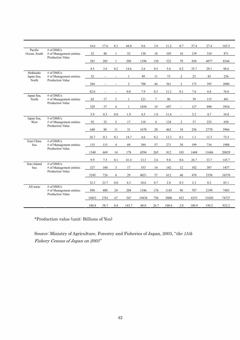
Table A2. Catch value and number of DMU classified by the fishery type and sea area Fishery type Total

Area 1 2 3 4 5 6 7 8 9 10

40 - - 1 66 13 91 - 38 45 294

504 - - 1 1199 102 637 - 259 234 2936

Hokkaido Pacific

Ocean, North

# of DMUs # of Management entities Production Value

23.8 - - 1.5 21.1 12.1 26.5 - 6.5 7.7 99.2

67 49 - 11 119 33 105 - 58 111 553

494 429 - 29 1500 80 447 - 269 1003 4251

Pacific Ocean, North

# of DMUs # of Management entities Production Value

20.4 5.8 - 21.3 5.9 6.3 17.9 - 58.5 19.2 155.2

91 67 8 35 214 17 138 26 72 325 993 Pacific Ocean, Middle

# of DMUs # of Management entities Production Value

1312 607 31 67 2806 43 458 184 382 3707 9597

42

14.6 17.6 0.1 44.0 9.6 3.0 11.2 0.7 37.4 27.4 165.5

52 48 1 52 130 18 105 16 139 310 871

383 205 1 209 1398 120 322 79 850 4977 8544

Pacific Ocean, South

# of DMUs # of Management entities Production Value

4.5 3.6 0.2 14.6 2.6 0.5 5.6 0.2 35.7 29.1 96.6

32 - - 1 49 11 73 2 23 45 236

204 - - 2 700 44 561 2 172 395 2080

Hokkaido Japan Sea,

North

# of DMUs # of Management entities Production Value

42.6 - - 0.0 7.9 0.3 11.2 0.1 7.6 6.8 76.6

62 17 3 1 121 7 96 - 39 115 461

329 37 4 1 1850 19 697 - 127 890 3954

Japan Sea, North

# of DMUs # of Management entities Production Value

5.9 0.3 0.0 1.9 4.5 1.0 11.4 - 5.2 4.7 34.8

92 32 5 17 110 6 124 2 37 225 650

640 88 11 31 1670 20 462 18 256 2770 5966

Japan Sea, West

# of DMUs # of Management entities Production Value

26.7 0.3 0.1 14.7 4.6 0.2 12.3 0.1 1.1 13.3 73.5

135 115 4 69 384 57 271 38 199 716 1988

1340 669 14 178 4294 265 812 103 1468 11686 20829

East China Sea

# of DMUs # of Management entities Production Value

9.9 7.5 0.1 41.4 13.3 2.6 9.8 0.6 26.7 33.7 145.7

327 160 3 17 353 14 142 12 102 307 1437

5245 726 6 29 4021 57 612 46 470 5358 16570

Seto Inland Sea

# of DMUs # of Management entities Production Value

32.3 23.7 0.0 4.3 10.6 0.7 2.8 0.3 2.3 8.2 85.1

898 488 24 204 1546 176 1145 96 707 2199 7483

10451 2761 67 547 19438 750 5008 432 4253 31020 74727

All areas # of DMUs # of Management entities Production Value

180.8 58.7 0.4 143.7 80.0 26.7 108.6 2.0 180.9 150.2 932.2

*Production value (unit: Billions of Yen) Source: Ministry of Agriculture, Forestry and Fisheries of Japan, 2003, “the 11th Fishery Census of Japan on 2003”

43

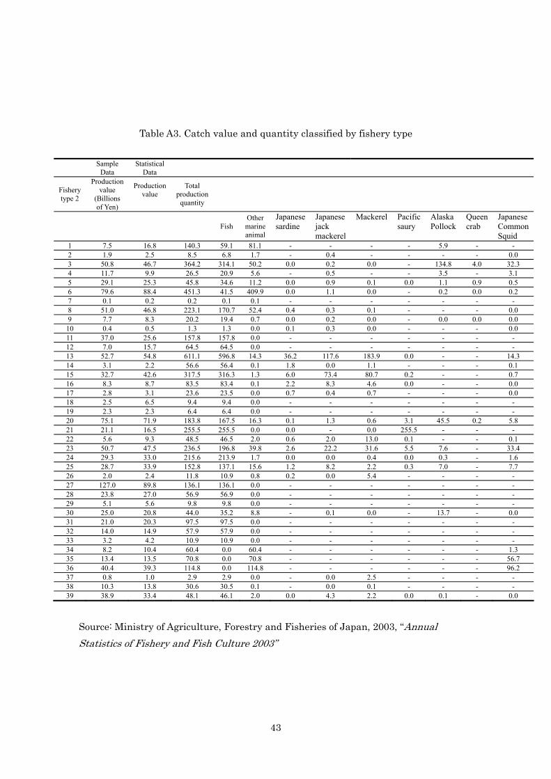
Table A3. Catch value and quantity classified by fishery type

Sample Data

Statistical Data

Fishery type 2

Production value

(Billions of Yen)

Production value

Total production

quantity

FishOther marine animal

Japanese sardine

Japanese jack mackerel

Mackerel Pacific saury

Alaska Pollock

Queen crab

Japanese Common Squid

1 7.5 16.8 140.3 59.1 81.1 - - - - 5.9 - - 2 1.9 2.5 8.5 6.8 1.7 - 0.4 - - - - 0.0 3 50.8 46.7 364.2 314.1 50.2 0.0 0.2 0.0 - 134.8 4.0 32.3 4 11.7 9.9 26.5 20.9 5.6 - 0.5 - - 3.5 - 3.1 5 29.1 25.3 45.8 34.6 11.2 0.0 0.9 0.1 0.0 1.1 0.9 0.5 6 79.6 88.4 451.3 41.5 409.9 0.0 1.1 0.0 - 0.2 0.0 0.2 7 0.1 0.2 0.2 0.1 0.1 - - - - - - - 8 51.0 46.8 223.1 170.7 52.4 0.4 0.3 0.1 - - - 0.0 9 7.7 8.3 20.2 19.4 0.7 0.0 0.2 0.0 - 0.0 0.0 0.0 10 0.4 0.5 1.3 1.3 0.0 0.1 0.3 0.0 - - - 0.0 11 37.0 25.6 157.8 157.8 0.0 - - - - - - - 12 7.0 15.7 64.5 64.5 0.0 - - - - - - - 13 52.7 54.8 611.1 596.8 14.3 36.2 117.6 183.9 0.0 - - 14.3 14 3.1 2.2 56.6 56.4 0.1 1.8 0.0 1.1 - - - 0.1 15 32.7 42.6 317.5 316.3 1.3 6.0 73.4 80.7 0.2 - - 0.7 16 8.3 8.7 83.5 83.4 0.1 2.2 8.3 4.6 0.0 - - 0.0 17 2.8 3.1 23.6 23.5 0.0 0.7 0.4 0.7 - - - 0.0 18 2.5 6.5 9.4 9.4 0.0 - - - - - - - 19 2.3 2.3 6.4 6.4 0.0 - - - - - - - 20 75.1 71.9 183.8 167.5 16.3 0.1 1.3 0.6 3.1 45.5 0.2 5.8 21 21.1 16.5 255.5 255.5 0.0 0.0 - 0.0 255.5 - - - 22 5.6 9.3 48.5 46.5 2.0 0.6 2.0 13.0 0.1 - - 0.1 23 50.7 47.5 236.5 196.8 39.8 2.6 22.2 31.6 5.5 7.6 - 33.4 24 29.3 33.0 215.6 213.9 1.7 0.0 0.0 0.4 0.0 0.3 - 1.6 25 28.7 33.9 152.8 137.1 15.6 1.2 8.2 2.2 0.3 7.0 - 7.7 26 2.0 2.4 11.8 10.9 0.8 0.2 0.0 5.4 - - - - 27 127.0 89.8 136.1 136.1 0.0 - - - - - - - 28 23.8 27.0 56.9 56.9 0.0 - - - - - - - 29 5.1 5.6 9.8 9.8 0.0 - - - - - - - 30 25.0 20.8 44.0 35.2 8.8 - 0.1 0.0 - 13.7 - 0.0 31 21.0 20.3 97.5 97.5 0.0 - - - - - - - 32 14.0 14.9 57.9 57.9 0.0 - - - - - - - 33 3.2 4.2 10.9 10.9 0.0 - - - - - - - 34 8.2 10.4 60.4 0.0 60.4 - - - - - - 1.3 35 13.4 13.5 70.8 0.0 70.8 - - - - - - 56.7 36 40.4 39.3 114.8 0.0 114.8 - - - - - - 96.2 37 0.8 1.0 2.9 2.9 0.0 - 0.0 2.5 - - - - 38 10.3 13.8 30.6 30.5 0.1 - 0.0 0.1 - - - - 39 38.9 33.4 48.1 46.1 2.0 0.0 4.3 2.2 0.0 0.1 - 0.0

Source: Ministry of Agriculture, Forestry and Fisheries of Japan, 2003, “Annual Statistics of Fishery and Fish Culture 2003”

44

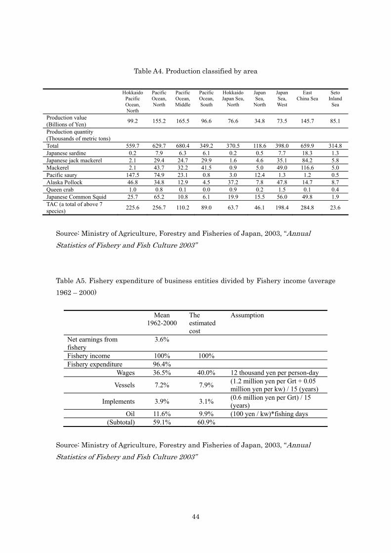
Table A4. Production classified by area

Hokkaido Pacific Ocean, North

Pacific Ocean, North

Pacific Ocean, Middle

Pacific Ocean, South

Hokkaido Japan Sea,

North

Japan Sea,

North

Japan Sea, West

East China Sea

Seto Inland

Sea

Production value (Billions of Yen) 99.2 155.2 165.5 96.6 76.6 34.8 73.5 145.7 85.1

Production quantity (Thousands of metric tons)

Total 559.7 629.7 680.4 349.2 370.5 118.6 398.0 659.9 314.8 Japanese sardine 0.2 7.9 6.3 6.1 0.2 0.5 7.7 18.3 1.3 Japanese jack mackerel 2.1 29.4 24.7 29.9 1.6 4.6 35.1 84.2 5.8 Mackerel 2.1 43.7 32.2 41.5 0.9 5.0 49.0 116.6 5.0 Pacific saury 147.5 74.9 23.1 0.8 3.0 12.4 1.3 1.2 0.5 Alaska Pollock 46.8 34.8 12.9 4.5 37.2 7.8 47.8 14.7 8.7 Queen crab 1.0 0.8 0.1 0.0 0.9 0.2 1.5 0.1 0.4 Japanese Common Squid 25.7 65.2 10.8 6.1 19.9 15.5 56.0 49.8 1.9 TAC (a total of above 7 species) 225.6 256.7 110.2 89.0 63.7 46.1 198.4 284.8 23.6

Source: Ministry of Agriculture, Forestry and Fisheries of Japan, 2003, “Annual Statistics of Fishery and Fish Culture 2003”

Table A5. Fishery expenditure of business entities divided by Fishery income (average 1962 – 2000)

Mean 1962-2000

The estimated cost

Assumption

Net earnings from fishery

3.6%

Fishery income 100% 100% Fishery expenditure 96.4%

Wages 36.5% 40.0% 12 thousand yen per person-day

Vessels 7.2% 7.9% (1.2 million yen per Grt + 0.05 million yen per kw) / 15 (years)

Implements 3.9% 3.1% (0.6 million yen per Grt) / 15 (years)

Oil 11.6% 9.9% (100 yen / kw)*fishing days (Subtotal) 59.1% 60.9%

Source: Ministry of Agriculture, Forestry and Fisheries of Japan, 2003, “Annual Statistics of Fishery and Fish Culture 2003”

45

Detailed Appendix Tables (A6-A9)

46

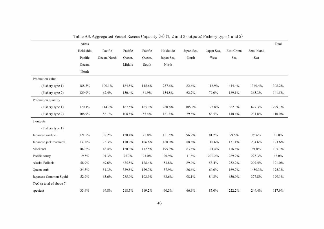
Table A6. Aggregated Vessel Excess Capacity (%) (1, 2 and 3 outputs; Fishery type 1 and 2) Areas Total

Hokkaido

Pacific

Ocean,

North

Pacific

Ocean, North

Pacific

Ocean,

Middle

Pacific

Ocean,

South

Hokkaido

Japan Sea,

North

Japan Sea,

North

Japan Sea,

West

East China

Sea

Seto Inland

Sea

Production value

(Fishery type 1) 188.3% 100.1% 184.5% 145.6% 237.6% 82.6% 116.9% 444.4% 1340.4% 308.2%

(Fishery type 2) 129.9% 62.4% 150.4% 61.9% 154.8% 62.7% 79.0% 189.1% 365.3% 141.5%

Production quantity

(Fishery type 1) 170.1% 114.7% 167.5% 165.9% 260.6% 105.2% 125.8% 362.3% 627.3% 229.1%

(Fishery type 2) 108.9% 58.1% 108.8% 55.4% 161.4% 59.8% 63.5% 140.4% 231.8% 110.0%

2 outputs

(Fishery type 1)

Japanese sardine 121.5% 38.2% 120.4% 71.8% 151.5% 96.2% 81.2% 99.5% 95.6% 86.0%

Japanese jack mackerel 137.0% 75.3% 170.9% 106.6% 168.0% 88.6% 110.6% 131.1% 234.6% 123.6%

Mackerel 102.2% 46.4% 150.3% 112.5% 195.9% 63.8% 101.4% 116.6% 91.0% 105.7%

Pacific saury 19.5% 94.3% 75.7% 93.0% 20.9% 11.8% 200.2% 289.7% 225.3% 48.0%

Alaska Pollock 58.9% 69.6% 675.5% 128.4% 53.8% 89.9% 53.4% 252.2% 297.4% 121.0%

Queen crab 24.3% 51.3% 339.5% 129.7% 37.9% 86.6% 60.0% 169.7% 1450.3% 175.3%

Japanese Common Squid 52.9% 65.6% 285.0% 103.9% 63.6% 98.1% 84.8% 650.0% 377.8% 199.1%

TAC (a total of above 7

species) 33.4% 69.8% 218.3% 119.2% 60.3% 66.9% 85.0% 222.2% 249.4% 117.9%

47

Other marine animals

(non-TAC species) 181.8% 94.3% 128.7% 141.8% 198.4% 88.1% 117.3% 206.8% 593.7% 196.7%

(Fishery type 2)

TAC (a total of above 7

species) 29.7% 60.3% 164.1% 54.6% 53.7% 51.2% 58.0% 177.4% 229.6% 91.2%

Other marine animals

(non-TAC species) 162.4% 56.5% 98.1% 55.7% 183.8% 65.2% 68.9% 112.4% 232.0% 118.7%

3 outputs

(Fishery type 1)

Japanese sardine 118.4% 36.6% 118.5% 70.0% 149.4% 91.5% 80.2% 97.6% 87.9% 84.1%

Japanese jack mackerel 135.3% 72.0% 169.6% 105.9% 165.6% 84.9% 108.3% 129.6% 197.9% 120.8%

Mackerel 74.6% 45.6% 148.8% 108.8% 116.9% 62.9% 98.9% 113.1% 75.0% 102.3%

Pacific saury 19.5% 94.3% 75.6% 92.5% 16.9% 11.8% 199.6% 287.2% 224.8% 47.8%

Alaska Pollock 57.0% 67.8% 673.1% 127.3% 52.7% 88.9% 52.6% 251.8% 293.8% 119.6%

Queen crab 50.8% 59.7% 272.9% 93.5% 60.2% 93.9% 81.0% 639.4% 353.6% 175.0%

Japanese Common

Squid 24.3% 51.2% 339.3% 129.6% 37.9% 86.2% 59.6% 169.7% 1448.9% 193.0%

TAC (a total of above 7

species) 32.3% 67.0% 177.0% 70.3% 56.9% 64.5% 69.5% 187.8% 235.5% 99.9%

Other fishes (non-TAC

species) 110.5% 85.7% 117.3% 121.9% 153.8% 75.7% 92.3% 142.2% 294.4% 129.4%

Other marine animals

(non-TAC species) 369.9% 73.8% 107.5% 110.9% 222.9% 92.4% 83.6% 289.4% 322.6% 224.0%

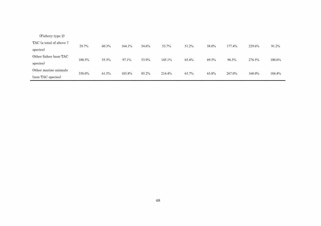
48

(Fishery type 2)

TAC (a total of above 7

species) 29.7% 60.3% 164.1% 54.6% 53.7% 51.2% 58.0% 177.4% 229.6% 91.2%

Other fishes (non-TAC

species) 100.5% 55.5% 97.1% 53.9% 145.1% 65.4% 69.5% 96.5% 276.5% 100.6%

Other marine animals

(non-TAC species) 358.0% 61.5% 103.8% 85.2% 214.4% 63.7% 63.8% 267.0% 168.0% 184.4%

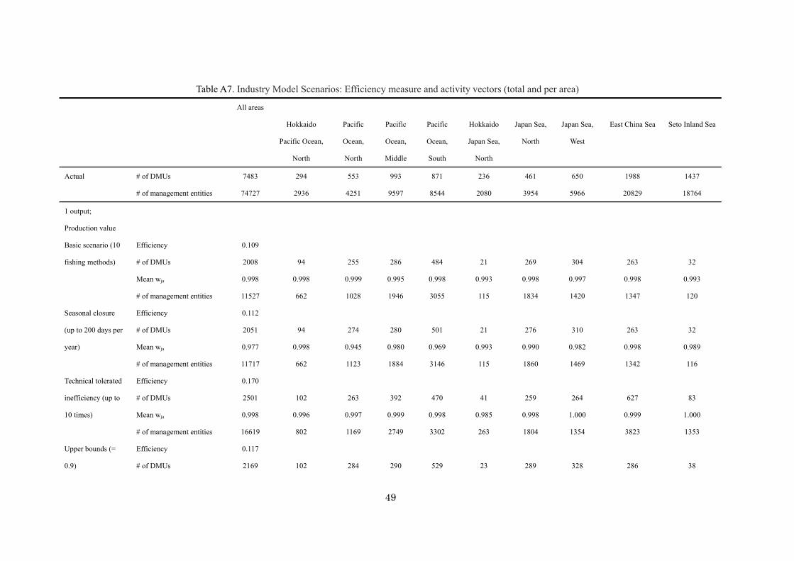
49

Table A7. Industry Model Scenarios: Efficiency measure and activity vectors (total and per area)

All areas

Hokkaido

Pacific Ocean,

North

Pacific

Ocean,

North

Pacific

Ocean,

Middle

Pacific

Ocean,

South

Hokkaido

Japan Sea,

North

Japan Sea,

North

Japan Sea,

West

East China Sea Seto Inland Sea

Actual # of DMUs

# of management entities

7483

74727

294

2936

553

4251

993

9597

871

8544

236

2080

461

3954

650

5966

1988

20829

1437

18764

1 output;

Production value

Basic scenario (10

fishing methods)

Efficiency

# of DMUs

Mean wja

# of management entities

0.109

2008

0.998

11527

94

0.998

662

255

0.999

1028

286

0.995

1946

484

0.998

3055

21

0.993

115

269

0.998

1834

304

0.997

1420

263

0.998

1347

32

0.993

120

Seasonal closure

(up to 200 days per

year)

Efficiency

# of DMUs

Mean wja

# of management entities

0.112

2051

0.977

11717

94

0.998

662

274

0.945

1123

280

0.980

1884

501

0.969

3146

21

0.993

115

276

0.990

1860

310

0.982

1469

263

0.998

1342

32

0.989

116

Technical tolerated

inefficiency (up to

10 times)

Efficiency

# of DMUs

Mean wja

# of management entities

0.170

2501

0.998

16619

102

0.996

802

263

0.997

1169

392

0.999

2749

470

0.998

3302

41

0.985

263

259

0.998

1804

264

1.000

1354

627

0.999

3823

83

1.000

1353

Upper bounds (=

0.9)

Efficiency

# of DMUs

0.117

2169

102

284

290

529

23

289

328

286

38

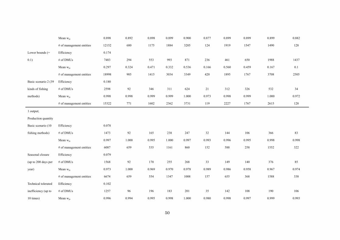
50

Mean wja

# of management entities

0.898

12152

0.892

680

0.898

1175

0.899

1884

0.900

3205

0.877

124

0.899

1919

0.899

1547

0.899

1490

0.882

128

Lower bounds (=

0.1)

Efficiency

# of DMUs

Mean wja

# of management entities

0.174

7483

0.297

18998

294

0.324

905

553

0.471

1415

993

0.332

3034

871

0.536

3349

236

0.166

420

461

0.560

1895

650

0.459

1767

1988

0.167

3708

1437

0.1

2505

Basic scenario 2 (39

kinds of fishing

methods)

Efficiency

# of DMUs

Mean wja

# of management entities

0.180

2598

0.998

15322

92

0.998

771

346

0.999

1602

311

0.999

2362

624

1.000

3731

21

0.973

119

312

0.998

2227

326

0.999

1767

532

1.000

2615

34

0.972

128

1 output;

Production quantity

Basic scenario (10

fishing methods)

Efficiency

# of DMUs

Mean wja

# of management entities

0.078

1473

0.997

6087

92

1.000

659

165

0.995

535

238

1.000

1161

247

0.997

860

32

0.993

152

144

0.996

588

106

0.995

258

366

0.998

1552

83

0.998

322

Seasonal closure

(up to 200 days per

year)

Efficiency

# of DMUs

Mean wja

# of management entities

0.079

1568

0.973

6674

92

1.000

659

170

0.969

554

255

0.970

1347

268

0.978

1008

33

0.989

157

149

0.986

655

140

0.958

368

376

0.967

1588

85

0.974

338

Technical tolerated

inefficiency (up to

10 times)

Efficiency

# of DMUs

Mean wja

0.102

1257

0.996

96

0.994

196

0.995

183

0.998

201

1.000

35

0.980

142

0.998

108

0.997

190

0.999

106

0.993

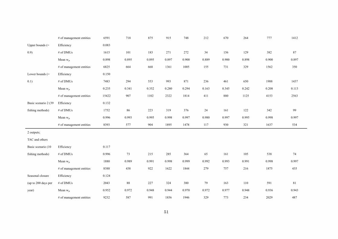
51

# of management entities 6591 718 875 915 748 212 670 264 777 1412

Upper bounds (=

0.9)

Efficiency

# of DMUs

Mean wja

# of management entities

0.083

1615

0.898

6825

101

0.895

664

183

0.895

668

271

0.897

1361

272

0.900

1005

34

0.889

155

156

0.900

731

129

0.898

329

382

0.900

1562

87

0.897

350

Lower bounds (=

0.1)

Efficiency

# of DMUs

Mean wja

# of management entities

0.150

7483

0.235

15422

294

0.341

907

553

0.352

1102

993

0.280

2322

871

0.294

1814

236

0.163

411

461

0.345

880

650

0.242

1125

1988

0.208

4153

1437

0.113

2563

Basic scenario 2 (39

fishing methods)

Efficiency

# of DMUs

Mean wja

# of management entities

0.132

1752

0.996

8393

86

0.993

577

223

0.995

904

319

0.998

1895

376

0.997

1478

24

0.980

117

161

0.997

930

122

0.995

321

342

0.998

1637

99

0.997

534

2 outputs;

TAC and others

Basic scenario (10

fishing methods)

Efficiency

# of DMUs

Mean wja

# of management entities

0.117

0.996

1880

8388

73

0.989

438

215

0.991

922

285

0.998

1622

364

0.999

1844

65

0.992

279

161

0.993

757

105

0.991

216

538

0.998

1875

74

0.997

435

Seasonal closure

(up to 200 days per

year)

Efficiency

# of DMUs

Mean wja

# of management entities

0.124

2043

0.952

9232

88

0.972

587

227

0.948

991

324

0.944

1856

380

0.970

1946

79

0.972

329

163

0.977

773

110

0.948

234

591

0.936

2029

81

0.943

487

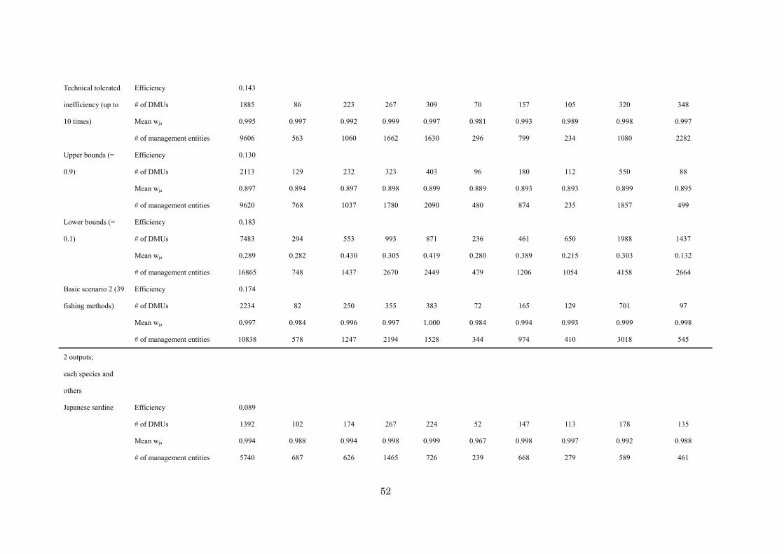
52

Technical tolerated

inefficiency (up to

10 times)

Efficiency

# of DMUs

Mean wja

# of management entities

0.143

1885

0.995

9606

86

0.997

563

223

0.992

1060

267

0.999

1662

309

0.997

1630

70

0.981

296

157

0.993

799

105

0.989

234

320

0.998

1080

348

0.997

2282

Upper bounds (=

0.9)

Efficiency

# of DMUs

Mean wja

# of management entities

0.130

2113

0.897

9620

129

0.894

768

232

0.897

1037

323

0.898

1780

403

0.899

2090

96

0.889

480

180

0.893

874

112

0.893

235

550

0.899

1857

88

0.895

499

Lower bounds (=

0.1)

Efficiency

# of DMUs

Mean wja

# of management entities

0.183

7483

0.289

16865

294

0.282

748

553

0.430

1437

993

0.305

2670

871

0.419

2449

236

0.280

479

461

0.389

1206

650

0.215

1054

1988

0.303

4158

1437

0.132

2664

Basic scenario 2 (39

fishing methods)

Efficiency

# of DMUs

Mean wja

# of management entities

0.174

2234

0.997

10838

82

0.984

578

250

0.996

1247

355

0.997

2194

383

1.000

1528

72

0.984

344

165

0.994

974

129

0.993

410

701

0.999

3018

97

0.998

545

2 outputs;

each species and

others

Japanese sardine Efficiency

# of DMUs

Mean wja

# of management entities

0.089

1392

0.994

5740

102

0.988

687

174

0.994

626

267

0.998

1465

224

0.999

726

52

0.967

239

147

0.998

668

113

0.997

279

178

0.992

589

135

0.988

461

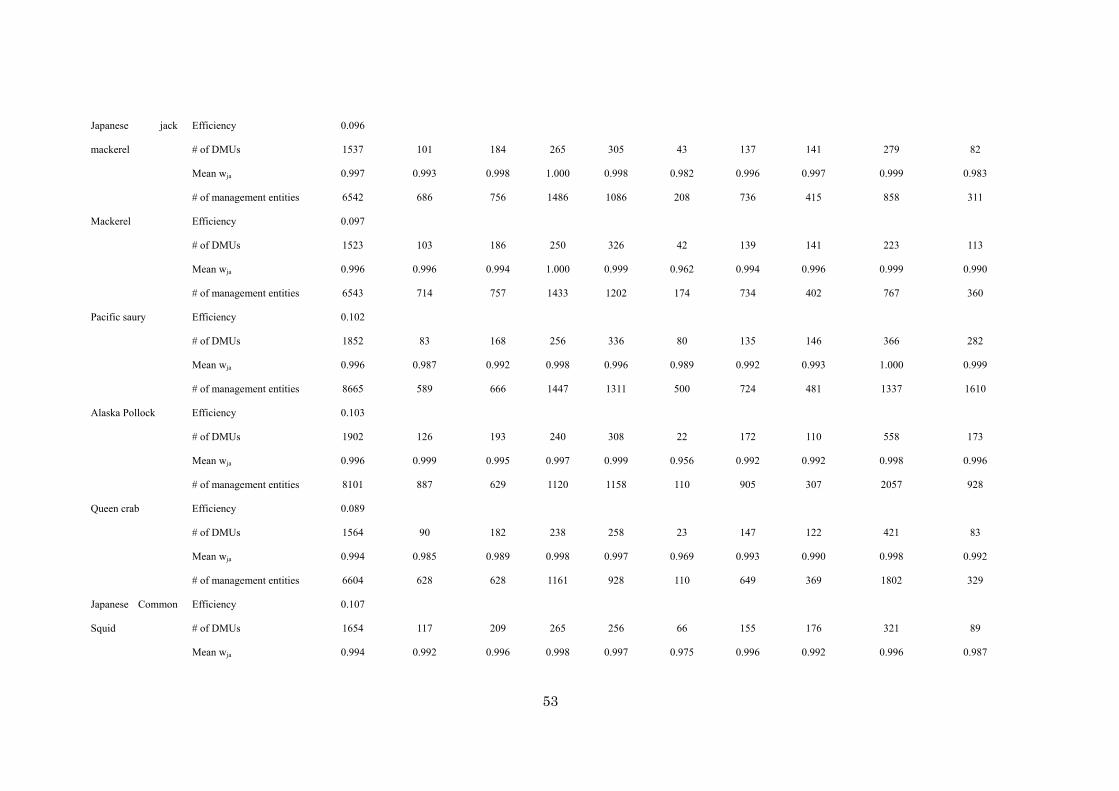
53

Japanese jack

mackerel

Efficiency

# of DMUs

Mean wja

# of management entities

0.096

1537

0.997

6542

101

0.993

686

184

0.998

756

265

1.000

1486

305

0.998

1086

43

0.982

208

137

0.996

736

141

0.997

415

279

0.999

858

82

0.983

311

Mackerel Efficiency

# of DMUs

Mean wja

# of management entities

0.097

1523

0.996

6543

103

0.996

714

186

0.994

757

250

1.000

1433

326

0.999

1202

42

0.962

174

139

0.994

734

141

0.996

402

223

0.999

767

113

0.990

360

Pacific saury Efficiency

# of DMUs

Mean wja

# of management entities

0.102

1852

0.996

8665

83

0.987

589

168

0.992

666

256

0.998

1447

336

0.996

1311

80

0.989

500

135

0.992

724

146

0.993

481

366

1.000

1337

282

0.999

1610

Alaska Pollock Efficiency

# of DMUs

Mean wja

# of management entities

0.103

1902

0.996

8101

126

0.999

887

193

0.995

629

240

0.997

1120

308

0.999

1158

22

0.956

110

172

0.992

905

110

0.992

307

558

0.998

2057

173

0.996

928

Queen crab Efficiency

# of DMUs

Mean wja

# of management entities

0.089

1564

0.994

6604

90

0.985

628

182

0.989

628

238

0.998

1161

258

0.997

928

23

0.969

110

147

0.993

649

122

0.990

369

421

0.998

1802

83

0.992

329

Japanese Common

Squid

Efficiency

# of DMUs

Mean wja

0.107

1654

0.994

117

0.992

209

0.996

265

0.998

256

0.997

66

0.975

155

0.996

176

0.992

321

0.996

89

0.987

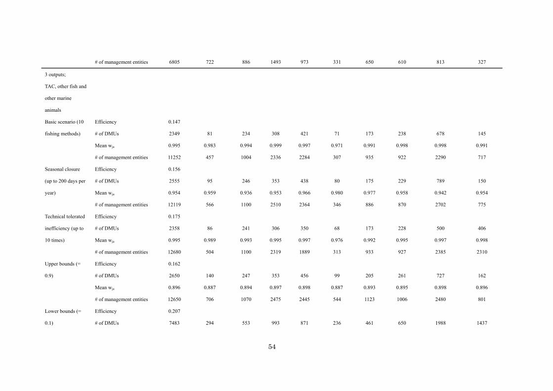
54

# of management entities 6805 722 886 1493 973 331 650 610 813 327

3 outputs;

TAC, other fish and

other marine

animals

Basic scenario (10

fishing methods)

Efficiency

# of DMUs

Mean wja

# of management entities

0.147

2349

0.995

11252

81

0.983

457

234

0.994

1004

308

0.999

2336

421

0.997

2284

71

0.971

307

173

0.991

935

238

0.998

922

678

0.998

2290

145

0.991

717

Seasonal closure

(up to 200 days per

year)

Efficiency

# of DMUs

Mean wja

# of management entities

0.156

2555

0.954

12119

95

0.959

566

246

0.936

1100

353

0.953

2510

438

0.966

2364

80

0.980

346

175

0.977

886

229

0.958

870

789

0.942

2702

150

0.954

775

Technical tolerated

inefficiency (up to

10 times)

Efficiency

# of DMUs

Mean wja

# of management entities

0.175

2358

0.995

12680

86

0.989

504

241

0.993

1100

306

0.995

2319

350

0.997

1889

68

0.976

313

173

0.992

933

228

0.995

927

500

0.997

2385

406

0.998

2310

Upper bounds (=

0.9)

Efficiency

# of DMUs

Mean wja

# of management entities

0.162

2650

0.896

12650

140

0.887

706

247

0.894

1070

353

0.897

2475

456

0.898

2445

99

0.887

544

205

0.893

1123

261

0.895

1006

727

0.898

2480

162

0.896

801

Lower bounds (=

0.1)

Efficiency

# of DMUs

0.207

7483

294

553

993

871

236

461

650

1988

1437

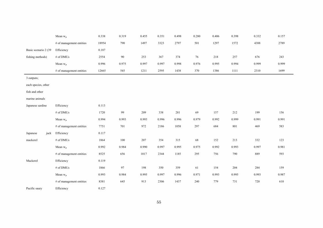
55

Mean wja

# of management entities

0.338

18954

0.319

790

0.455

1497

0.351

3323

0.498

2797

0.280

501

0.406

1297

0.398

1572

0.332

4388

0.157

2789

Basic scenario 2 (39

fishing methods)

Efficiency

# of DMUs

Mean wja

# of management entities

0.187

2554

0.996

12665

90

0.975

545

253

0.997

1211

367

0.997

2595

374

0.998

1438

76

0.976

370

218

0.995

1386

257

0.994

1111

676

0.999

2310

243

0.999

1699

3 outputs;

each species, other

fish and other

marine animals

Japanese sardine Efficiency

# of DMUs

Mean wja

# of management entities

0.113

1720

0.994

7751

99

0.993

701

209

0.993

972

338

0.996

2186

281

0.996

1058

69

0.979

297

157

0.992

684

212

0.999

801

199

0.991

469

156

0.991

583

Japanese jack

mackerel

Efficiency

# of DMUs

Mean wja

# of management entities

0.117

1864

0.992

8525

100

0.984

656

207

0.990

1017

354

0.997

2344

315

0.995

1185

68

0.975

295

152

0.992

756

213

0.993

790

332

0.997

889

123

0.981

593

Mackerel Efficiency

# of DMUs

Mean wja

# of management entities

0.119

1866

0.993

8381

97

0.984

645

198

0.995

913

350

0.997

2306

359

0.996

1437

61

0.971

240

154

0.993

779

204

0.995

731

284

0.993

720

159

0.987

610

Pacific saury Efficiency 0.127

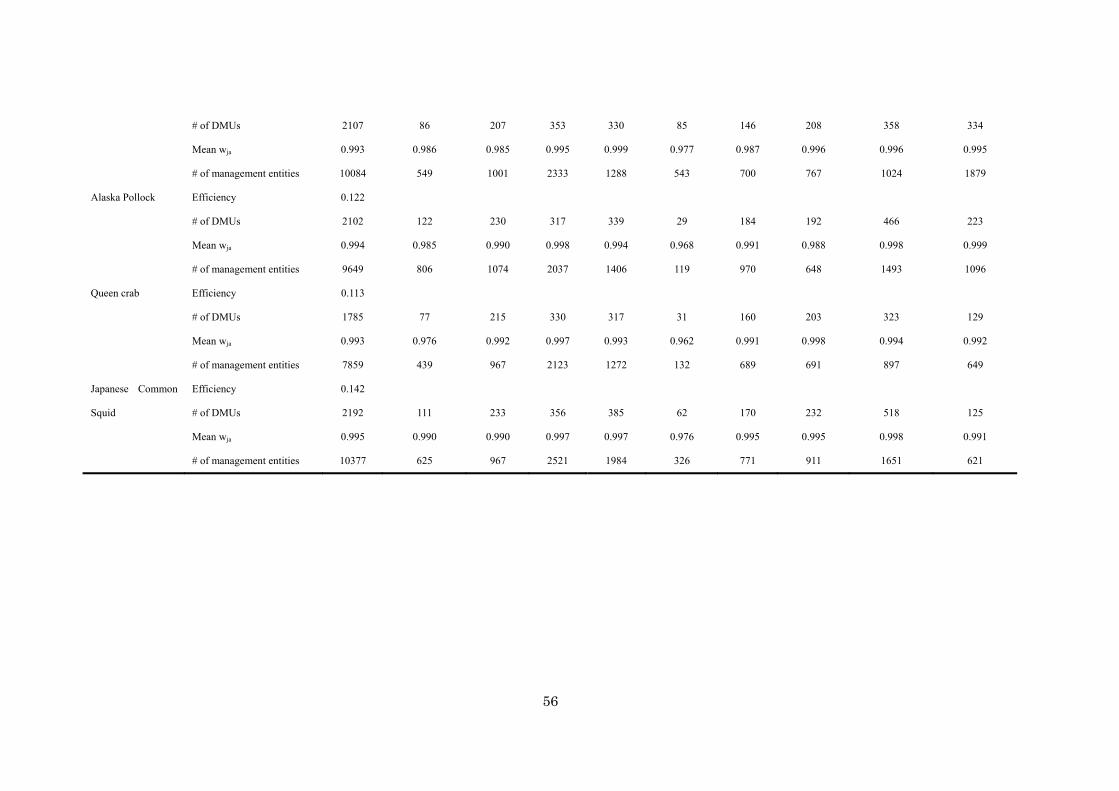
56

# of DMUs

Mean wja

# of management entities

2107

0.993

10084

86

0.986

549

207

0.985

1001

353

0.995

2333

330

0.999

1288

85

0.977

543

146

0.987

700

208

0.996

767

358

0.996

1024

334

0.995

1879

Alaska Pollock Efficiency

# of DMUs

Mean wja

# of management entities

0.122

2102

0.994

9649

122

0.985

806

230

0.990

1074

317

0.998

2037

339

0.994

1406

29

0.968

119

184

0.991

970

192

0.988

648

466

0.998

1493

223

0.999

1096

Queen crab Efficiency

# of DMUs

Mean wja

# of management entities

0.113

1785

0.993

7859

77

0.976

439

215

0.992

967

330

0.997

2123

317

0.993

1272

31

0.962

132

160

0.991

689

203

0.998

691

323

0.994

897

129

0.992

649

Japanese Common

Squid

Efficiency

# of DMUs

Mean wja

# of management entities

0.142

2192

0.995

10377

111

0.990

625

233

0.990

967

356

0.997

2521

385

0.997

1984

62

0.976

326

170

0.995

771

232

0.995

911

518

0.998

1651

125

0.991

621

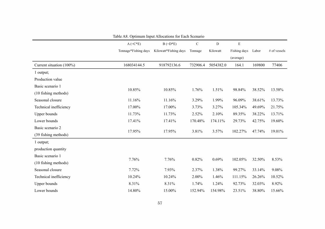
57

Table A8. Optimum Input Allocations for Each Scenario

A (=C*E) B (=D*E) C D E

Tonnage*Fishing days Kilowatt*Fishing days Tonnage Kilowatt Fishing days

(average)

Labor # of vessels

Current situation (100%) 168034144.5 918792136.6 732906.4 5054382.0 164.1 169800 77406

1 output;

Production value

Basic scenario 1

(10 fishing methods) 10.85% 10.85% 1.76% 1.51% 98.84% 38.52% 13.58%

Seasonal closure 11.16% 11.16% 3.29% 1.99% 96.09% 38.61% 13.73%

Technical inefficiency 17.00% 17.00% 3.73% 3.27% 105.34% 49.69% 21.75%

Upper bounds 11.73% 11.73% 2.52% 2.10% 89.35% 38.22% 13.71%

Lower bounds 17.41% 17.41% 170.48% 174.11% 29.73% 42.75% 19.60%

Basic scenario 2

(39 fishing methods) 17.95% 17.95% 3.81% 3.57% 102.27% 47.74% 19.01%

1 output;

production quantity

Basic scenario 1

(10 fishing methods) 7.76% 7.76% 0.82% 0.69% 102.05% 32.50% 8.53%

Seasonal closure 7.72% 7.93% 2.37% 1.38% 99.27% 33.14% 9.08%

Technical inefficiency 10.24% 10.24% 2.00% 1.46% 111.15% 26.26% 10.52%

Upper bounds 8.31% 8.31% 1.74% 1.24% 92.73% 32.03% 8.92%

Lower bounds 14.80% 15.00% 152.94% 154.98% 23.51% 38.80% 15.66%

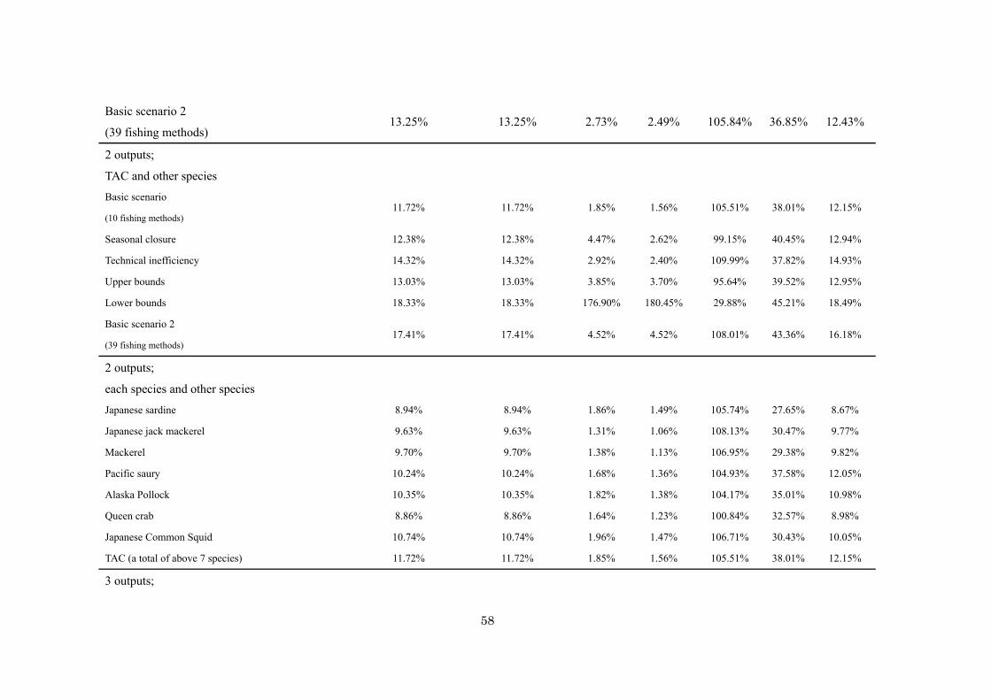
58

Basic scenario 2

(39 fishing methods) 13.25% 13.25% 2.73% 2.49% 105.84% 36.85% 12.43%

2 outputs;

TAC and other species

Basic scenario

(10 fishing methods) 11.72% 11.72% 1.85% 1.56% 105.51% 38.01% 12.15%

Seasonal closure 12.38% 12.38% 4.47% 2.62% 99.15% 40.45% 12.94%

Technical inefficiency 14.32% 14.32% 2.92% 2.40% 109.99% 37.82% 14.93%

Upper bounds 13.03% 13.03% 3.85% 3.70% 95.64% 39.52% 12.95%

Lower bounds 18.33% 18.33% 176.90% 180.45% 29.88% 45.21% 18.49%

Basic scenario 2

(39 fishing methods) 17.41% 17.41% 4.52% 4.52% 108.01% 43.36% 16.18%

2 outputs;

each species and other species

Japanese sardine 8.94% 8.94% 1.86% 1.49% 105.74% 27.65% 8.67%

Japanese jack mackerel 9.63% 9.63% 1.31% 1.06% 108.13% 30.47% 9.77%

Mackerel 9.70% 9.70% 1.38% 1.13% 106.95% 29.38% 9.82%

Pacific saury 10.24% 10.24% 1.68% 1.36% 104.93% 37.58% 12.05%

Alaska Pollock 10.35% 10.35% 1.82% 1.38% 104.17% 35.01% 10.98%

Queen crab 8.86% 8.86% 1.64% 1.23% 100.84% 32.57% 8.98%

Japanese Common Squid 10.74% 10.74% 1.96% 1.47% 106.71% 30.43% 10.05%

TAC (a total of above 7 species) 11.72% 11.72% 1.85% 1.56% 105.51% 38.01% 12.15%

3 outputs;

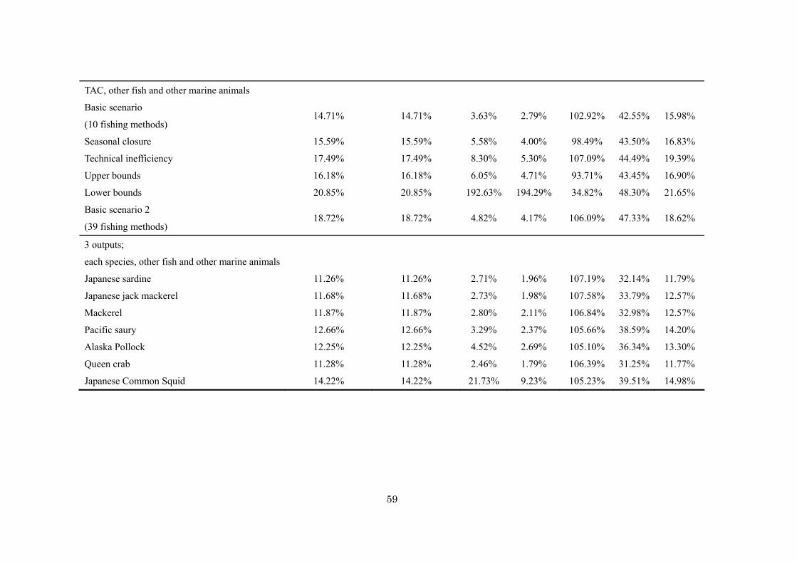
59

TAC, other fish and other marine animals

Basic scenario

(10 fishing methods) 14.71% 14.71% 3.63% 2.79% 102.92% 42.55% 15.98%

Seasonal closure 15.59% 15.59% 5.58% 4.00% 98.49% 43.50% 16.83%

Technical inefficiency 17.49% 17.49% 8.30% 5.30% 107.09% 44.49% 19.39%

Upper bounds 16.18% 16.18% 6.05% 4.71% 93.71% 43.45% 16.90%

Lower bounds 20.85% 20.85% 192.63% 194.29% 34.82% 48.30% 21.65%

Basic scenario 2

(39 fishing methods) 18.72% 18.72% 4.82% 4.17% 106.09% 47.33% 18.62%

3 outputs;

each species, other fish and other marine animals

Japanese sardine 11.26% 11.26% 2.71% 1.96% 107.19% 32.14% 11.79%

Japanese jack mackerel 11.68% 11.68% 2.73% 1.98% 107.58% 33.79% 12.57%

Mackerel 11.87% 11.87% 2.80% 2.11% 106.84% 32.98% 12.57%

Pacific saury 12.66% 12.66% 3.29% 2.37% 105.66% 38.59% 14.20%

Alaska Pollock 12.25% 12.25% 4.52% 2.69% 105.10% 36.34% 13.30%

Queen crab 11.28% 11.28% 2.46% 1.79% 106.39% 31.25% 11.77%

Japanese Common Squid 14.22% 14.22% 21.73% 9.23% 105.23% 39.51% 14.98%

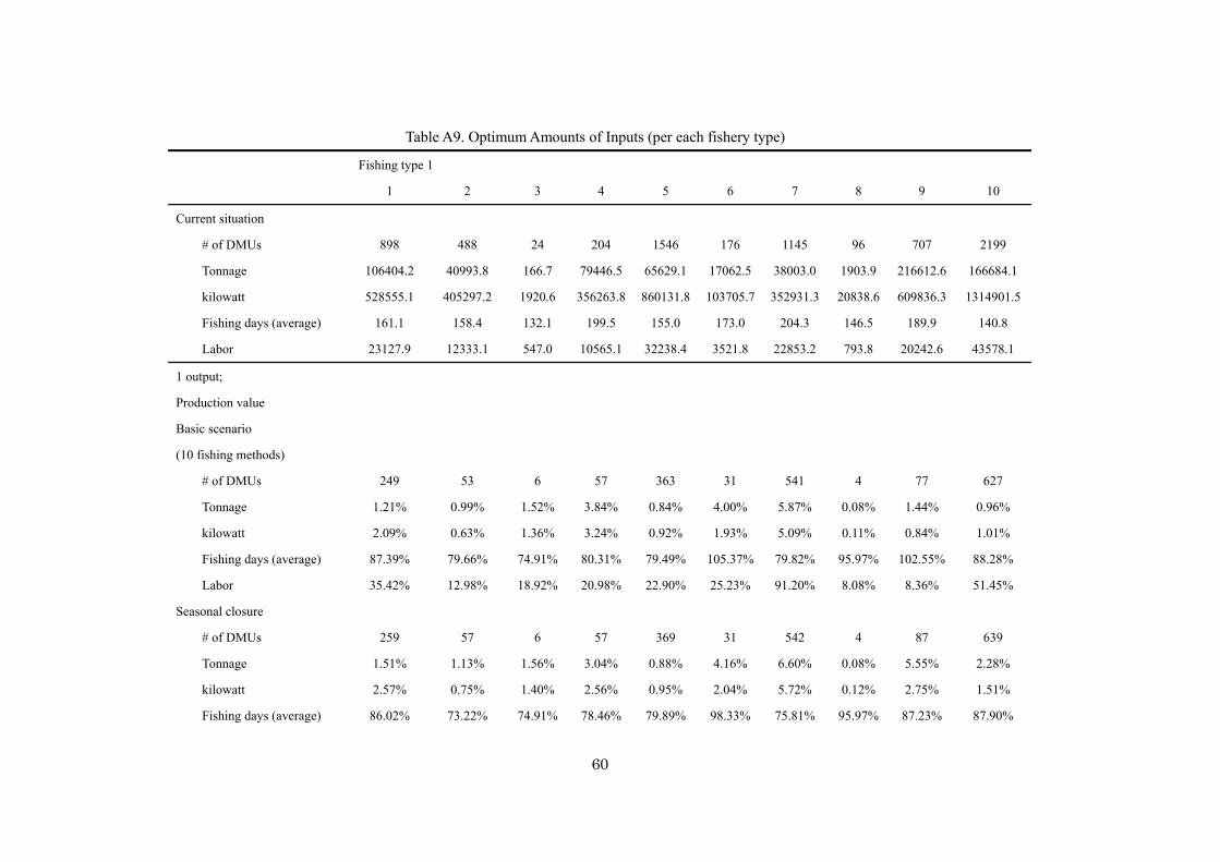
60

Table A9. Optimum Amounts of Inputs (per each fishery type)

Fishing type 1

1 2 3 4 5 6 7 8 9 10

Current situation

# of DMUs

Tonnage

kilowatt

Fishing days (average)

Labor

898

106404.2

528555.1

161.1

23127.9

488

40993.8

405297.2

158.4

12333.1

24

166.7

1920.6

132.1

547.0

204

79446.5

356263.8

199.5

10565.1

1546

65629.1

860131.8

155.0

32238.4

176

17062.5

103705.7

173.0

3521.8

1145

38003.0

352931.3

204.3

22853.2

96

1903.9

20838.6

146.5

793.8

707

216612.6

609836.3

189.9

20242.6

2199

166684.1

1314901.5

140.8

43578.1

1 output;

Production value

Basic scenario

(10 fishing methods)

# of DMUs

Tonnage

kilowatt

Fishing days (average)

Labor

249

1.21%

2.09%

87.39%

35.42%

53

0.99%

0.63%

79.66%

12.98%

6

1.52%

1.36%

74.91%

18.92%

57

3.84%

3.24%

80.31%

20.98%

363

0.84%

0.92%

79.49%

22.90%

31

4.00%

1.93%

105.37%

25.23%

541

5.87%

5.09%

79.82%

91.20%

4

0.08%

0.11%

95.97%

8.08%

77

1.44%

0.84%

102.55%

8.36%

627

0.96%

1.01%

88.28%

51.45%

Seasonal closure

# of DMUs

Tonnage

kilowatt

Fishing days (average)

259

1.51%

2.57%

86.02%

57

1.13%

0.75%

73.22%

6

1.56%

1.40%

74.91%

57

3.04%

2.56%

78.46%

369

0.88%

0.95%

79.89%

31

4.16%

2.04%

98.33%

542

6.60%

5.72%

75.81%

4

0.08%

0.12%

95.97%

87

5.55%

2.75%

87.23%

639

2.28%

1.51%

87.90%

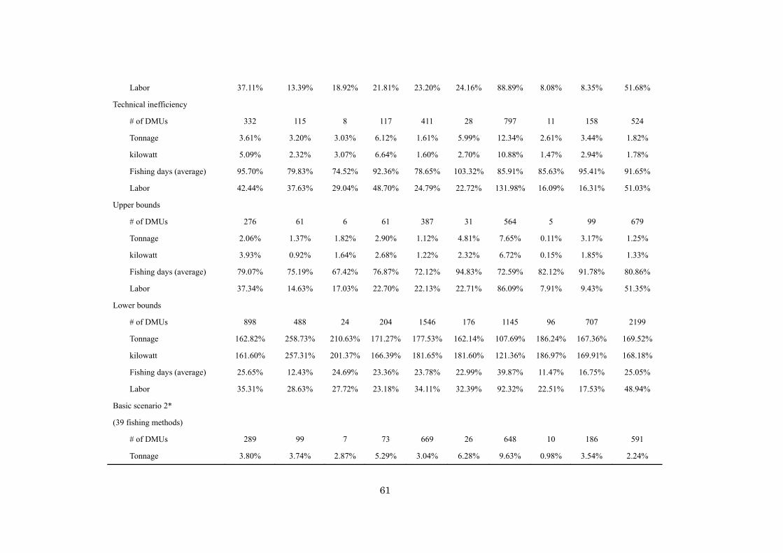
61

Labor 37.11% 13.39% 18.92% 21.81% 23.20% 24.16% 88.89% 8.08% 8.35% 51.68%

Technical inefficiency

# of DMUs

Tonnage

kilowatt

Fishing days (average)

Labor

332

3.61%

5.09%

95.70%

42.44%

115

3.20%

2.32%

79.83%

37.63%

8

3.03%

3.07%

74.52%

29.04%

117

6.12%

6.64%

92.36%

48.70%

411

1.61%

1.60%

78.65%

24.79%

28

5.99%

2.70%

103.32%

22.72%

797

12.34%

10.88%

85.91%

131.98%

11

2.61%

1.47%

85.63%

16.09%

158

3.44%

2.94%

95.41%

16.31%

524

1.82%

1.78%

91.65%

51.03%

Upper bounds

# of DMUs

Tonnage

kilowatt

Fishing days (average)

Labor

276

2.06%

3.93%

79.07%

37.34%

61

1.37%

0.92%

75.19%

14.63%

6

1.82%

1.64%

67.42%

17.03%

61

2.90%

2.68%

76.87%

22.70%

387

1.12%

1.22%

72.12%

22.13%

31

4.81%

2.32%

94.83%

22.71%

564

7.65%

6.72%

72.59%

86.09%

5

0.11%

0.15%

82.12%

7.91%

99

3.17%

1.85%

91.78%

9.43%

679

1.25%

1.33%

80.86%

51.35%

Lower bounds

# of DMUs

Tonnage

kilowatt

Fishing days (average)

Labor

898

162.82%

161.60%

25.65%

35.31%

488

258.73%

257.31%

12.43%

28.63%

24

210.63%

201.37%

24.69%

27.72%

204

171.27%

166.39%

23.36%

23.18%

1546

177.53%

181.65%

23.78%

34.11%

176

162.14%

181.60%

22.99%

32.39%

1145

107.69%

121.36%

39.87%

92.32%

96

186.24%

186.97%

11.47%

22.51%

707

167.36%

169.91%

16.75%

17.53%

2199

169.52%

168.18%

25.05%

48.94%

Basic scenario 2*

(39 fishing methods)

# of DMUs

Tonnage

289

3.80%

99

3.74%

7

2.87%

73

5.29%

669

3.04%

26

6.28%

648

9.63%

10

0.98%

186

3.54%

591

2.24%

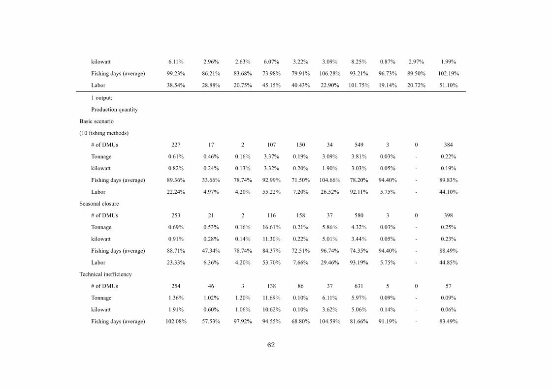
62

kilowatt

Fishing days (average)

Labor

6.11%

99.23%

38.54%

2.96%

86.21%

28.88%

2.63%

83.68%

20.75%

6.07%

73.98%

45.15%

3.22%

79.91%

40.43%

3.09%

106.28%

22.90%

8.25%

93.21%

101.75%

0.87%

96.73%

19.14%

2.97%

89.50%

20.72%

1.99%

102.19%

51.10%

1 output;

Production quantity

Basic scenario

(10 fishing methods)

# of DMUs

Tonnage

kilowatt

Fishing days (average)

Labor

227

0.61%

0.82%

89.36%

22.24%

17

0.46%

0.24%

33.66%

4.97%

2

0.16%

0.13%

78.74%

4.20%

107

3.37%

3.32%

92.99%

55.22%

150

0.19%

0.20%

71.50%

7.20%

34

3.09%

1.90%

104.66%

26.52%

549

3.81%

3.03%

78.20%

92.11%

3

0.03%

0.05%

94.40%

5.75%

0

-

-

-

-

384

0.22%

0.19%

89.83%

44.10%

Seasonal closure

# of DMUs

Tonnage

kilowatt

Fishing days (average)

Labor

253

0.69%

0.91%

88.71%

23.33%

21

0.53%

0.28%

47.34%

6.36%

2

0.16%

0.14%

78.74%

4.20%

116

16.61%

11.30%

84.37%

53.70%

158

0.21%

0.22%

72.51%

7.66%

37

5.86%

5.01%

96.74%

29.46%

580

4.32%

3.44%

74.35%

93.19%

3

0.03%

0.05%

94.40%

5.75%

0

-

-

-

-

398

0.25%

0.23%

88.49%

44.85%

Technical inefficiency

# of DMUs

Tonnage

kilowatt

Fishing days (average)

254

1.36%

1.91%

102.08%

46

1.02%

0.60%

57.53%

3

1.20%

1.06%

97.92%

138

11.69%

10.62%

94.55%

86

0.10%

0.10%

68.80%

37

6.11%

3.62%

104.59%

631

5.97%

5.06%

81.66%

5

0.09%

0.14%

91.19%

0

-

-

-

57

0.09%

0.06%

83.49%

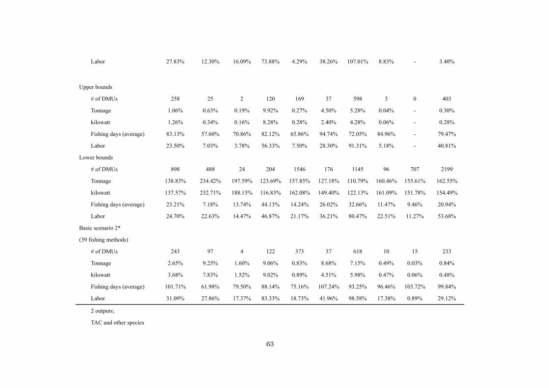
63

Labor 27.83% 12.30% 16.09% 73.88% 4.29% 38.26% 107.01% 8.83% - 3.40%

Upper bounds

# of DMUs

Tonnage

kilowatt

Fishing days (average)

Labor

258

1.06%

1.26%

83.13%

23.50%

25

0.63%

0.34%

57.60%

7.03%

2

0.19%

0.16%

70.86%

3.78%

120

9.92%

8.28%

82.12%

56.33%

169

0.27%

0.28%

65.86%

7.50%

37

4.50%

2.40%

94.74%

28.30%

598

5.28%

4.28%

72.05%

91.31%

3

0.04%

0.06%

84.96%

5.18%

0

-

-

-

-

403

0.30%

0.28%

79.47%

40.81%

Lower bounds

# of DMUs

Tonnage

kilowatt

Fishing days (average)

Labor

898

138.83%

137.57%

23.21%

24.70%

488

234.42%

232.71%

7.18%

22.63%

24

197.59%

188.15%

13.74%

14.47%

204

123.69%

116.83%

44.13%

46.87%

1546

157.85%

162.08%

14.24%

21.17%

176

127.18%

149.40%

26.02%

36.21%

1145

110.79%

122.13%

32.66%

80.47%

96

160.46%

161.09%

11.47%

22.51%

707

155.61%

151.78%

9.46%

11.27%

2199

162.55%

154.49%

20.94%

53.68%

Basic scenario 2*

(39 fishing methods)

# of DMUs

Tonnage

kilowatt

Fishing days (average)

Labor

243

2.65%

3.68%

101.71%

31.09%

97

9.25%

7.83%

61.98%

27.86%

4

1.60%

1.52%

79.50%

17.37%

122

9.06%

9.02%

88.14%

83.33%

373

0.83%

0.89%

75.16%

18.73%

37

8.68%

4.51%

107.24%

41.96%

618

7.15%

5.98%

93.25%

98.58%

10

0.49%

0.47%

96.46%

17.38%

15

0.03%

0.06%

103.72%

0.89%

233

0.84%

0.48%

99.84%

29.12%

2 outputs;

TAC and other species

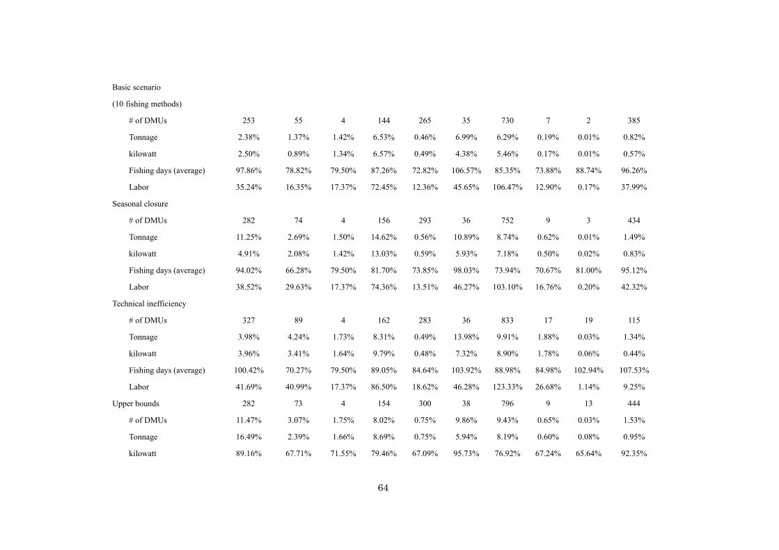
64

Basic scenario

(10 fishing methods)

# of DMUs

Tonnage

kilowatt

Fishing days (average)

Labor

253

2.38%

2.50%

97.86%

35.24%

55

1.37%

0.89%

78.82%

16.35%

4

1.42%

1.34%

79.50%

17.37%

144

6.53%

6.57%

87.26%

72.45%

265

0.46%

0.49%

72.82%

12.36%

35

6.99%

4.38%

106.57%

45.65%

730

6.29%

5.46%

85.35%

106.47%

7

0.19%

0.17%

73.88%

12.90%

2

0.01%

0.01%

88.74%

0.17%

385

0.82%

0.57%

96.26%

37.99%

Seasonal closure

# of DMUs

Tonnage

kilowatt

Fishing days (average)

Labor

282

11.25%

4.91%

94.02%

38.52%

74

2.69%

2.08%

66.28%

29.63%

4

1.50%

1.42%

79.50%

17.37%

156

14.62%

13.03%

81.70%

74.36%

293

0.56%

0.59%

73.85%

13.51%

36

10.89%

5.93%

98.03%

46.27%

752

8.74%

7.18%

73.94%

103.10%

9

0.62%

0.50%

70.67%

16.76%

3

0.01%

0.02%

81.00%

0.20%

434

1.49%

0.83%

95.12%

42.32%

Technical inefficiency

# of DMUs

Tonnage

kilowatt

Fishing days (average)

Labor

327

3.98%

3.96%

100.42%

41.69%

89

4.24%

3.41%

70.27%

40.99%

4

1.73%

1.64%

79.50%

17.37%

162

8.31%

9.79%

89.05%

86.50%

283

0.49%

0.48%

84.64%

18.62%

36

13.98%

7.32%

103.92%

46.28%

833

9.91%

8.90%

88.98%

123.33%

17

1.88%

1.78%

84.98%

26.68%

19

0.03%

0.06%

102.94%

1.14%

115

1.34%

0.44%

107.53%

9.25%

Upper bounds

# of DMUs

Tonnage

kilowatt

282

11.47%

16.49%

89.16%

73

3.07%

2.39%

67.71%

4

1.75%

1.66%

71.55%

154

8.02%

8.69%

79.46%

300

0.75%

0.75%

67.09%

38

9.86%

5.94%

95.73%

796

9.43%

8.19%

76.92%

9

0.65%

0.60%

67.24%

13

0.03%

0.08%

65.64%

444

1.53%

0.95%

92.35%

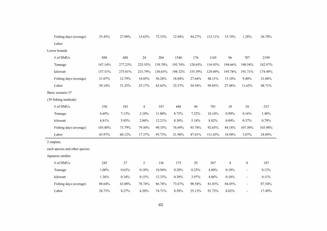
65

Fishing days (average)

Labor

35.45% 27.98% 15.63% 72.33% 12.94% 44.27% 112.11% 15.74% 1.28% 36.70%

Lower bounds

# of DMUs

Tonnage

kilowatt

Fishing days (average)

Labor

898

147.14%

157.51%

31.07%

39.14%

488

277.23%

275.81%

12.79%

31.25%

24

225.55%

215.79%

18.85%

25.17%

204

139.70%

130.63%

56.28%

65.65%

1546

193.74%

198.32%

18.04%

25.57%

176

128.65%

155.39%

27.64%

54.54%

1145

116.93%

129.49%

48.11%

99.85%

96

194.66%

195.78%

13.10%

27.48%

707

190.54%

191.71%

9.40%

11.65%

2199

182.97%

174.49%

21.68%

48.71%

Basic scenario 2*

(39 fishing methods)

# of DMUs

Tonnage

kilowatt

Fishing days (average)

Labor

330

6.69%

6.81%

103.80%

43.97%

183

7.13%

5.95%

73.79%

60.12%

4

2.10%

2.00%

79.50%

17.37%

147

11.80%

12.21%

90.35%

95.73%

448

8.75%

8.30%

76.69%

21.98%

44

7.22%

5.18%

93.70%

47.41%

781

10.14%

8.82%

92.65%

111.43%

10

0.99%

0.89%

84.18%

18.94%

34

0.16%

0.37%

107.30%

3.07%

253

1.48%

0.79%

103.98%

24.89%

2 outputs;

each species and other species

Japanese sardine

# of DMUs

Tonnage

kilowatt

Fishing days (average)

Labor

245

1.00%

1.36%

88.64%

24.73%

27

0.63%

0.34%

63.08%

8.27%

2

0.18%

0.15%

78.74%

4.20%

156

10.94%

12.33%

86.78%

74.71%

175

0.28%

0.30%

73.67%

8.58%

29

8.25%

3.97%

98.54%

25.13%

567

4.80%

4.06%

81.83%

91.72%

4

0.10%

0.10%

84.45%

8.02%

0

-

-

-

-

187

0.12%

0.11%

87.54%

17.49%

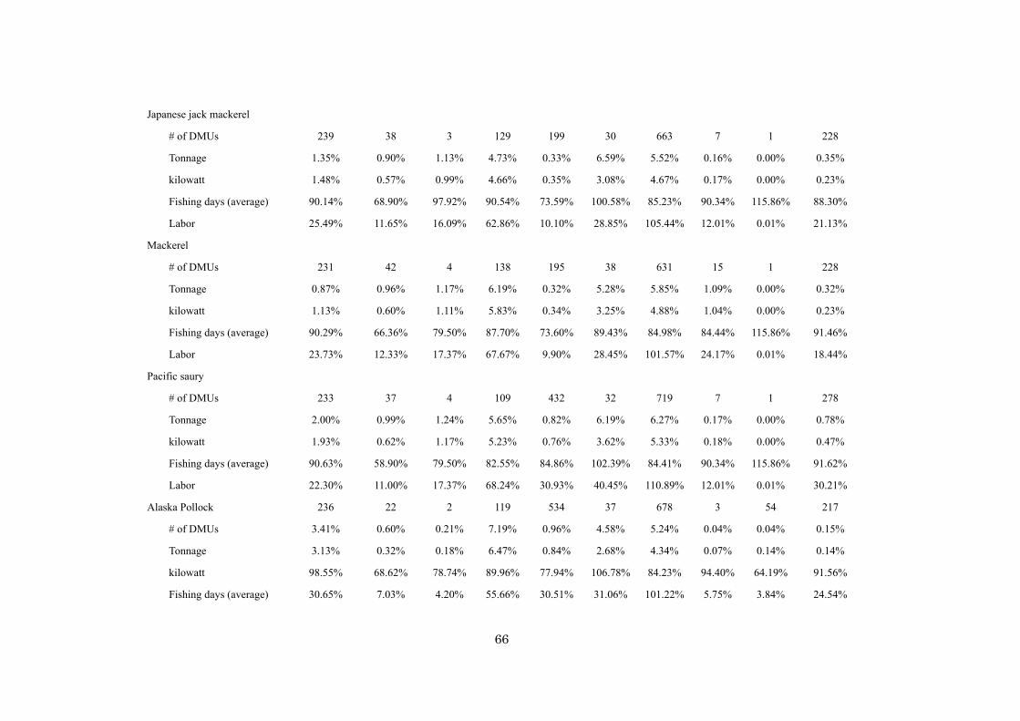
66

Japanese jack mackerel

# of DMUs

Tonnage

kilowatt

Fishing days (average)

Labor

239

1.35%

1.48%

90.14%

25.49%

38

0.90%

0.57%

68.90%

11.65%

3

1.13%

0.99%

97.92%

16.09%

129

4.73%

4.66%

90.54%

62.86%

199

0.33%

0.35%

73.59%

10.10%

30

6.59%

3.08%

100.58%

28.85%

663

5.52%

4.67%

85.23%

105.44%

7

0.16%

0.17%

90.34%

12.01%

1

0.00%

0.00%

115.86%

0.01%

228

0.35%

0.23%

88.30%

21.13%

Mackerel

# of DMUs

Tonnage

kilowatt

Fishing days (average)

Labor

231

0.87%

1.13%

90.29%

23.73%

42

0.96%

0.60%

66.36%

12.33%

4

1.17%

1.11%

79.50%

17.37%

138

6.19%

5.83%

87.70%

67.67%

195

0.32%

0.34%

73.60%

9.90%

38

5.28%

3.25%

89.43%

28.45%

631

5.85%

4.88%

84.98%

101.57%

15

1.09%

1.04%

84.44%

24.17%

1

0.00%

0.00%

115.86%

0.01%

228

0.32%

0.23%

91.46%

18.44%

Pacific saury

# of DMUs

Tonnage

kilowatt

Fishing days (average)

Labor

233

2.00%

1.93%

90.63%

22.30%

37

0.99%

0.62%

58.90%

11.00%

4

1.24%

1.17%

79.50%

17.37%

109

5.65%

5.23%

82.55%

68.24%

432

0.82%

0.76%

84.86%

30.93%

32

6.19%

3.62%

102.39%

40.45%

719

6.27%

5.33%

84.41%

110.89%

7

0.17%

0.18%

90.34%

12.01%

1

0.00%

0.00%

115.86%

0.01%

278

0.78%

0.47%

91.62%

30.21%

Alaska Pollock

# of DMUs

Tonnage

kilowatt

Fishing days (average)

236

3.41%

3.13%

98.55%

30.65%

22

0.60%

0.32%

68.62%

7.03%

2

0.21%

0.18%

78.74%

4.20%

119

7.19%

6.47%

89.96%

55.66%

534

0.96%

0.84%

77.94%

30.51%

37

4.58%

2.68%

106.78%

31.06%

678

5.24%

4.34%

84.23%

101.22%

3

0.04%

0.07%

94.40%

5.75%

54

0.04%

0.14%

64.19%

3.84%

217

0.15%

0.14%

91.56%

24.54%

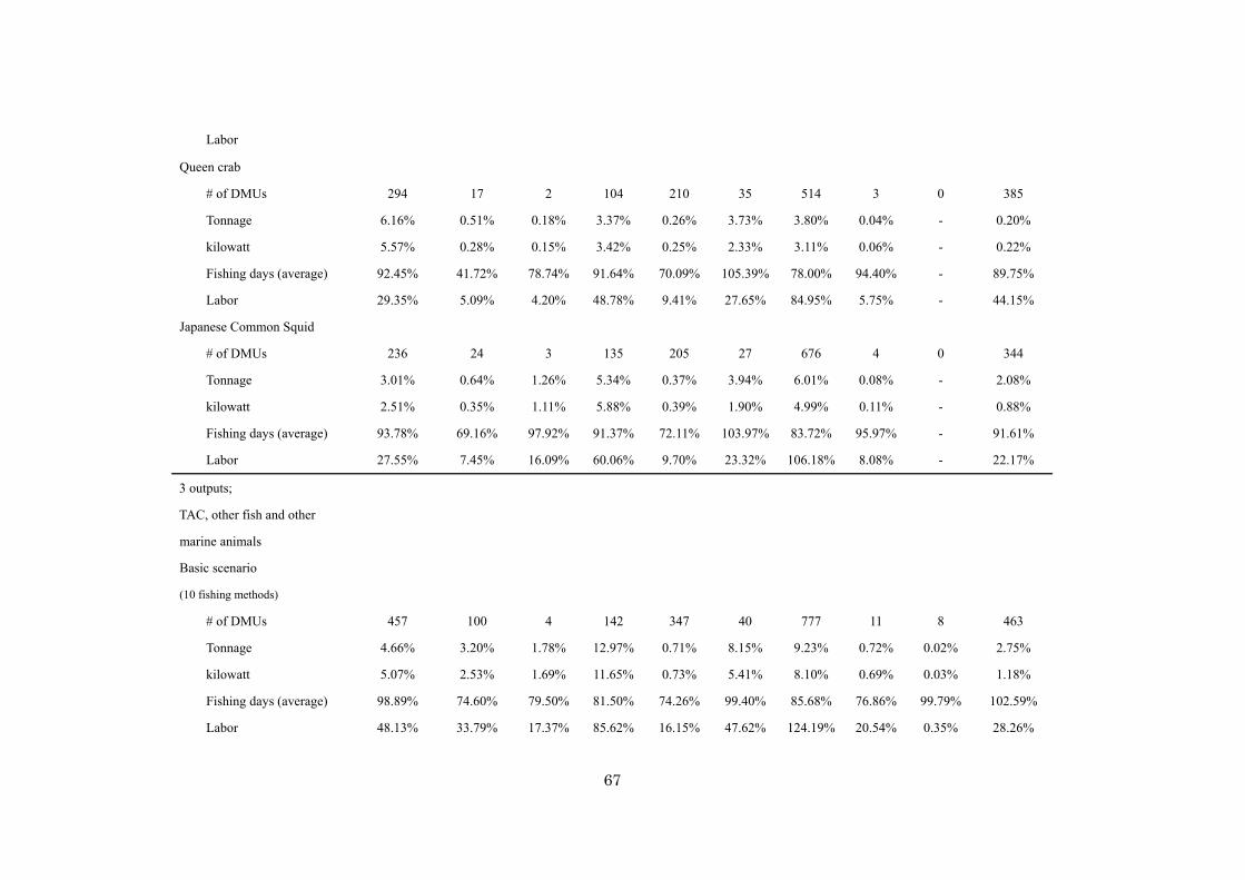
67

Labor

Queen crab

# of DMUs

Tonnage

kilowatt

Fishing days (average)

Labor

294

6.16%

5.57%

92.45%

29.35%

17

0.51%

0.28%

41.72%

5.09%

2

0.18%

0.15%

78.74%

4.20%

104

3.37%

3.42%

91.64%

48.78%

210

0.26%

0.25%

70.09%

9.41%

35

3.73%

2.33%

105.39%

27.65%

514

3.80%

3.11%

78.00%

84.95%

3

0.04%

0.06%

94.40%

5.75%

0

-

-

-

-

385

0.20%

0.22%

89.75%

44.15%

Japanese Common Squid

# of DMUs

Tonnage

kilowatt

Fishing days (average)

Labor

236

3.01%

2.51%

93.78%

27.55%

24

0.64%

0.35%

69.16%

7.45%

3

1.26%

1.11%

97.92%

16.09%

135

5.34%

5.88%

91.37%

60.06%

205

0.37%

0.39%

72.11%

9.70%

27

3.94%

1.90%

103.97%

23.32%

676

6.01%

4.99%

83.72%

106.18%

4

0.08%

0.11%

95.97%

8.08%

0

-

-

-

-

344

2.08%

0.88%

91.61%

22.17%

3 outputs;

TAC, other fish and other

marine animals

Basic scenario

(10 fishing methods)

# of DMUs

Tonnage

kilowatt

Fishing days (average)

Labor

457

4.66%

5.07%

98.89%

48.13%

100

3.20%

2.53%

74.60%

33.79%

4

1.78%

1.69%

79.50%

17.37%

142

12.97%

11.65%

81.50%

85.62%

347

0.71%

0.73%

74.26%

16.15%

40

8.15%

5.41%

99.40%

47.62%

777

9.23%

8.10%

85.68%

124.19%

11

0.72%

0.69%

76.86%

20.54%

8

0.02%

0.03%

99.79%

0.35%

463

2.75%

1.18%

102.59%

28.26%

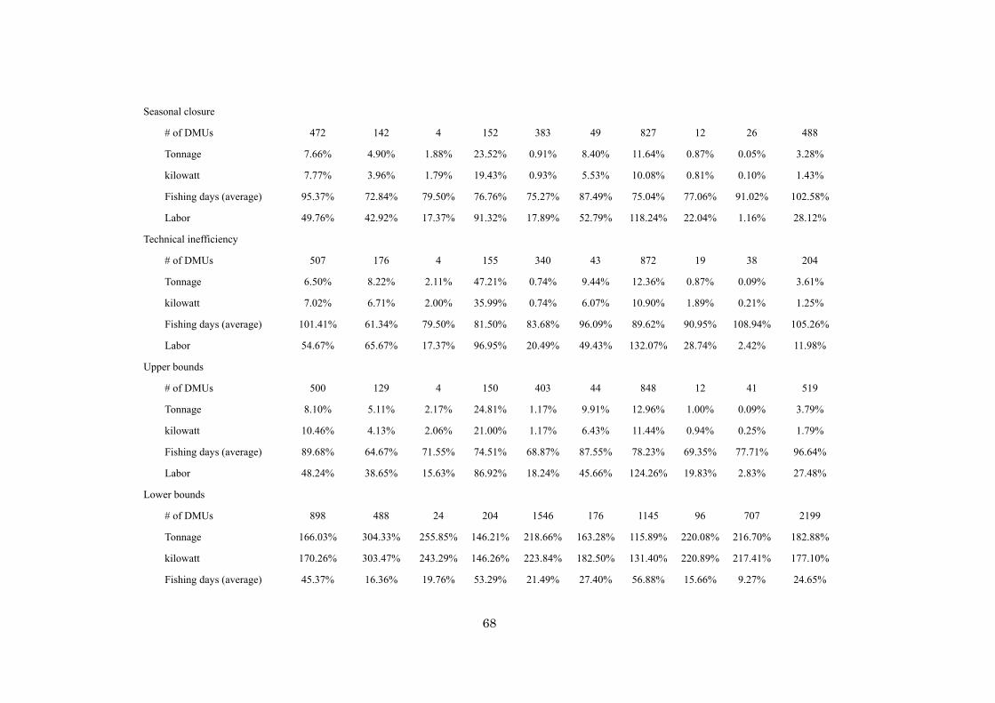
68

Seasonal closure

# of DMUs

Tonnage

kilowatt

Fishing days (average)

Labor

472

7.66%

7.77%

95.37%

49.76%

142

4.90%

3.96%

72.84%

42.92%

4

1.88%

1.79%

79.50%

17.37%

152

23.52%

19.43%

76.76%

91.32%

383

0.91%

0.93%

75.27%

17.89%

49

8.40%

5.53%

87.49%

52.79%

827

11.64%

10.08%

75.04%

118.24%

12

0.87%

0.81%

77.06%

22.04%

26

0.05%

0.10%

91.02%

1.16%

488

3.28%

1.43%

102.58%

28.12%

Technical inefficiency

# of DMUs

Tonnage

kilowatt

Fishing days (average)

Labor

507

6.50%

7.02%

101.41%

54.67%

176

8.22%

6.71%

61.34%

65.67%

4

2.11%

2.00%

79.50%

17.37%

155

47.21%

35.99%

81.50%

96.95%

340

0.74%

0.74%

83.68%

20.49%

43

9.44%

6.07%

96.09%

49.43%

872

12.36%

10.90%

89.62%

132.07%

19

0.87%

1.89%

90.95%

28.74%

38

0.09%

0.21%

108.94%

2.42%

204

3.61%

1.25%

105.26%

11.98%

Upper bounds

# of DMUs

Tonnage

kilowatt

Fishing days (average)

Labor

500

8.10%

10.46%

89.68%

48.24%

129

5.11%

4.13%

64.67%

38.65%

4

2.17%

2.06%

71.55%

15.63%

150

24.81%

21.00%

74.51%

86.92%

403

1.17%

1.17%

68.87%

18.24%

44

9.91%

6.43%

87.55%

45.66%

848

12.96%

11.44%

78.23%

124.26%

12

1.00%

0.94%

69.35%

19.83%

41

0.09%

0.25%

77.71%

2.83%

519

3.79%

1.79%

96.64%

27.48%

Lower bounds

# of DMUs

Tonnage

kilowatt

Fishing days (average)

898

166.03%

170.26%

45.37%

488

304.33%

303.47%

16.36%

24

255.85%

243.29%

19.76%

204

146.21%

146.26%

53.29%

1546

218.66%

223.84%

21.49%

176

163.28%

182.50%

27.40%

1145

115.89%

131.40%

56.88%

96

220.08%

220.89%

15.66%

707

216.70%

217.41%

9.27%

2199

182.88%

177.10%

24.65%

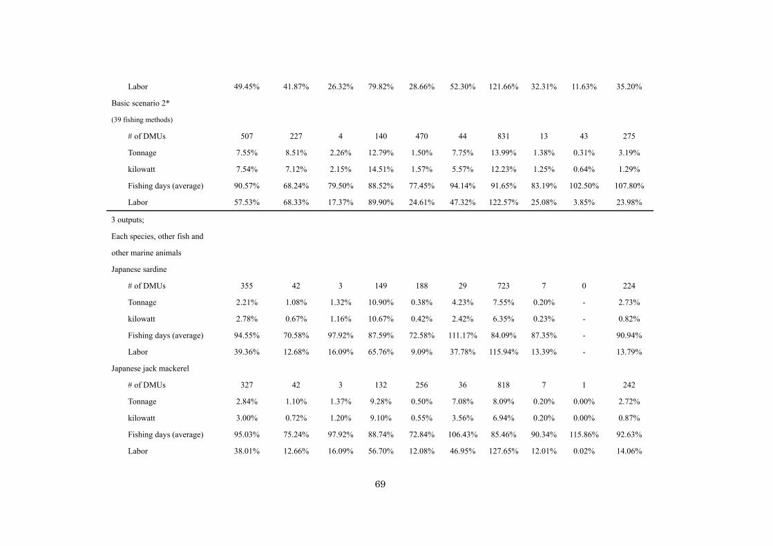
69

Labor 49.45% 41.87% 26.32% 79.82% 28.66% 52.30% 121.66% 32.31% 11.63% 35.20%

Basic scenario 2*

(39 fishing methods)

# of DMUs

Tonnage

kilowatt

Fishing days (average)

Labor

507

7.55%

7.54%

90.57%

57.53%

227

8.51%

7.12%

68.24%

68.33%

4

2.26%

2.15%

79.50%

17.37%

140

12.79%

14.51%

88.52%

89.90%

470

1.50%

1.57%

77.45%

24.61%

44

7.75%

5.57%

94.14%

47.32%

831

13.99%

12.23%

91.65%

122.57%

13

1.38%

1.25%

83.19%

25.08%

43

0.31%

0.64%

102.50%

3.85%

275

3.19%

1.29%

107.80%

23.98%

3 outputs;

Each species, other fish and

other marine animals

Japanese sardine

# of DMUs

Tonnage

kilowatt

Fishing days (average)

Labor

355

2.21%

2.78%

94.55%

39.36%

42

1.08%

0.67%

70.58%

12.68%

3

1.32%

1.16%

97.92%

16.09%

149

10.90%

10.67%

87.59%

65.76%

188

0.38%

0.42%

72.58%

9.09%

29

4.23%

2.42%

111.17%

37.78%

723

7.55%

6.35%

84.09%

115.94%

7

0.20%

0.23%

87.35%

13.39%

0

-

-

-

-

224

2.73%

0.82%

90.94%

13.79%

Japanese jack mackerel

# of DMUs

Tonnage

kilowatt

Fishing days (average)

Labor

327

2.84%

3.00%

95.03%

38.01%

42

1.10%

0.72%

75.24%

12.66%

3

1.37%

1.20%

97.92%

16.09%

132

9.28%

9.10%

88.74%

56.70%

256

0.50%

0.55%

72.84%

12.08%

36

7.08%

3.56%

106.43%

46.95%

818

8.09%

6.94%

85.46%

127.65%

7

0.20%

0.20%

90.34%

12.01%

1

0.00%

0.00%

115.86%

0.02%

242

2.72%

0.87%

92.63%

14.06%

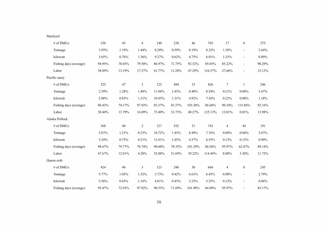
70

Mackerel

# of DMUs

Tonnage

kilowatt

Fishing days (average)

Labor

336

3.95%

3.65%

94.95%

38.89%

45

1.19%

0.76%

70.45%

13.19%

4

1.44%

1.36%

79.50%

17.37%

140

8.20%

9.27%

86.97%

61.77%

238

0.59%

0.62%

71.75%

11.28%

46

8.19%

4.75%

92.52%

47.29%

765

8.22%

6.91%

85.65%

116.57%

17

1.38%

1.33%

85.22%

27.66%

0

-

-

-

-

275

2.64%

0.89%

90.29%

15.13%

Pacific saury

# of DMUs

Tonnage

kilowatt

Fishing days (average)

Labor

325

2.59%

2.88%

96.42%

38.40%

47

1.28%

0.83%

74.17%

13.79%

3

1.48%

1.31%

97.92%

16.09%

125

11.84%

10.45%

83.37%

73.40%

494

1.43%

1.31%

83.37%

33.73%

33

8.40%

4.92%

103.30%

40.27%

826

8.54%

7.36%

86.68%

125.13%

7

0.21%

0.22%

90.34%

12.01%

1

0.00%

0.00%

115.86%

0.01%

246

3.47%

1.18%

92.16%

13.98%

Alaska Pollock

# of DMUs

Tonnage

kilowatt

Fishing days (average)

Labor

368

5.87%

5.24%

98.67%

47.67%

40

1.21%

0.75%

79.77%

12.01%

2

0.25%

0.21%

78.74%

4.20%

127

18.72%

13.41%

90.60%

52.88%

552

1.43%

1.45%

78.35%

31.69%

31

8.49%

4.57%

101.29%

39.22%

743

7.76%

6.55%

86.56%

114.44%

4

0.09%

0.13%

95.97%

8.08%

44

0.04%

0.15%

62.47%

3.30%

191

3.67%

0.90%

89.14%

11.72%

Queen crab

# of DMUs

Tonnage

kilowatt

Fishing days (average)

424

5.77%

5.56%

95.47%

40

1.03%

0.65%

72.93%

3

1.32%

1.16%

97.92%

123

3.73%

4.81%

90.53%

248

0.42%

0.43%

71.69%

30

6.61%

3.23%

101.90%

668

6.43%

5.25%

84.98%

4

0.08%

0.12%

95.97%

0

-

-

-

245

2.79%

0.86%

85.17%

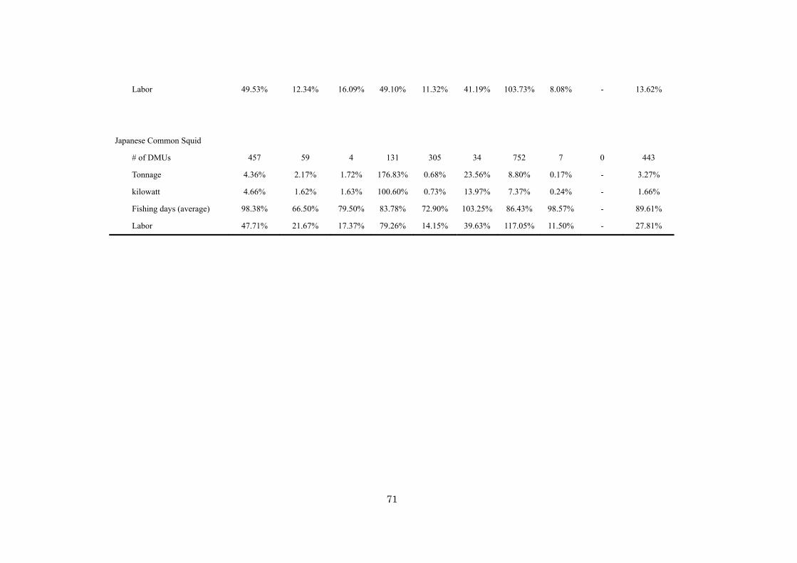
71

Labor 49.53% 12.34% 16.09% 49.10% 11.32% 41.19% 103.73% 8.08% - 13.62%

Japanese Common Squid

# of DMUs

Tonnage

kilowatt

Fishing days (average)

Labor

457

4.36%

4.66%

98.38%

47.71%

59

2.17%

1.62%

66.50%

21.67%

4

1.72%

1.63%

79.50%

17.37%

131

176.83%

100.60%

83.78%

79.26%

305

0.68%

0.73%

72.90%

14.15%

34

23.56%

13.97%

103.25%

39.63%

752

8.80%

7.37%

86.43%

117.05%

7

0.17%

0.24%

98.57%

11.50%

0

-

-

-

-

443

3.27%

1.66%

89.61%

27.81%

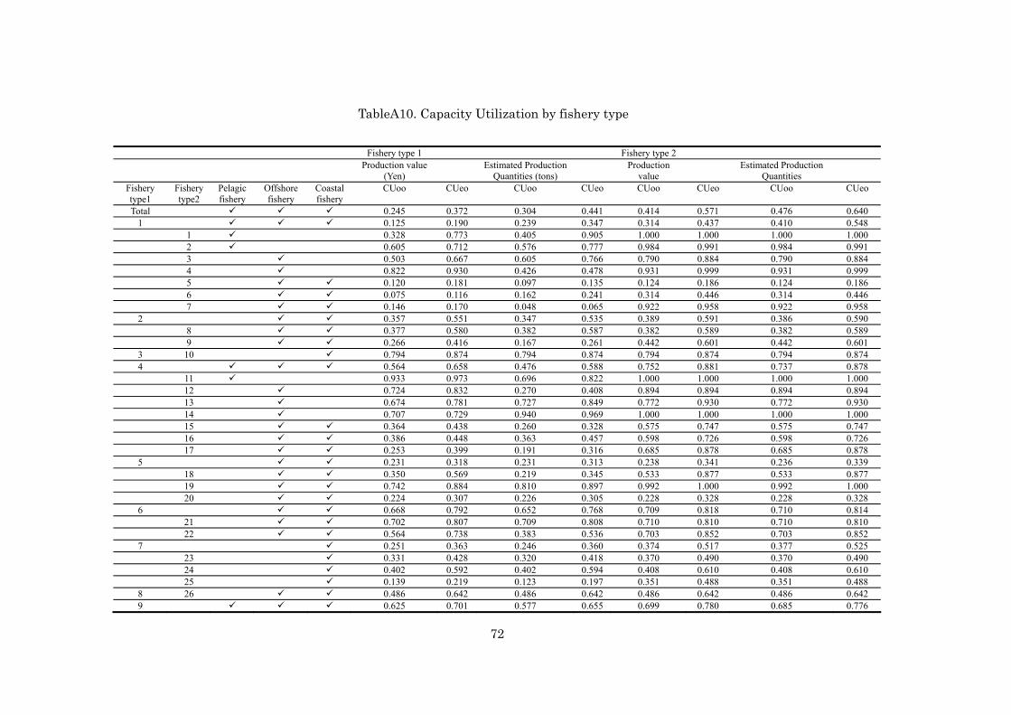
72

TableA10. Capacity Utilization by fishery type

Fishery type 1 Fishery type 2 Production value

(Yen) Estimated Production Quantities (tons)

Production value Estimated Production

Quantities

Fishery type1

Fisherytype2

Pelagic fishery

Offshore fishery

Coastalfishery

CUoo CUeo CUoo CUeo CUoo CUeo CUoo CUeo

Total 0.245 0.372 0.304 0.441 0.414 0.571 0.476 0.640 1 0.125 0.190 0.239 0.347 0.314 0.437 0.410 0.548 1 0.328 0.773 0.405 0.905 1.000 1.000 1.000 1.000 2 0.605 0.712 0.576 0.777 0.984 0.991 0.984 0.991 3 0.503 0.667 0.605 0.766 0.790 0.884 0.790 0.884 4 0.822 0.930 0.426 0.478 0.931 0.999 0.931 0.999 5 0.120 0.181 0.097 0.135 0.124 0.186 0.124 0.186 6 0.075 0.116 0.162 0.241 0.314 0.446 0.314 0.446 7 0.146 0.170 0.048 0.065 0.922 0.958 0.922 0.958

2 0.357 0.551 0.347 0.535 0.389 0.591 0.386 0.590 8 0.377 0.580 0.382 0.587 0.382 0.589 0.382 0.589 9 0.266 0.416 0.167 0.261 0.442 0.601 0.442 0.601

3 10 0.794 0.874 0.794 0.874 0.794 0.874 0.794 0.874 4 0.564 0.658 0.476 0.588 0.752 0.881 0.737 0.878 11 0.933 0.973 0.696 0.822 1.000 1.000 1.000 1.000 12 0.724 0.832 0.270 0.408 0.894 0.894 0.894 0.894 13 0.674 0.781 0.727 0.849 0.772 0.930 0.772 0.930 14 0.707 0.729 0.940 0.969 1.000 1.000 1.000 1.000 15 0.364 0.438 0.260 0.328 0.575 0.747 0.575 0.747 16 0.386 0.448 0.363 0.457 0.598 0.726 0.598 0.726 17 0.253 0.399 0.191 0.316 0.685 0.878 0.685 0.878

5 0.231 0.318 0.231 0.313 0.238 0.341 0.236 0.339 18 0.350 0.569 0.219 0.345 0.533 0.877 0.533 0.877 19 0.742 0.884 0.810 0.897 0.992 1.000 0.992 1.000 20 0.224 0.307 0.226 0.305 0.228 0.328 0.228 0.328

6 0.668 0.792 0.652 0.768 0.709 0.818 0.710 0.814 21 0.702 0.807 0.709 0.808 0.710 0.810 0.710 0.810 22 0.564 0.738 0.383 0.536 0.703 0.852 0.703 0.852

7 0.251 0.363 0.246 0.360 0.374 0.517 0.377 0.525 23 0.331 0.428 0.320 0.418 0.370 0.490 0.370 0.490 24 0.402 0.592 0.402 0.594 0.408 0.610 0.408 0.610 25 0.139 0.219 0.123 0.197 0.351 0.488 0.351 0.488

8 26 0.486 0.642 0.486 0.642 0.486 0.642 0.486 0.642 9 0.625 0.701 0.577 0.655 0.699 0.780 0.685 0.776

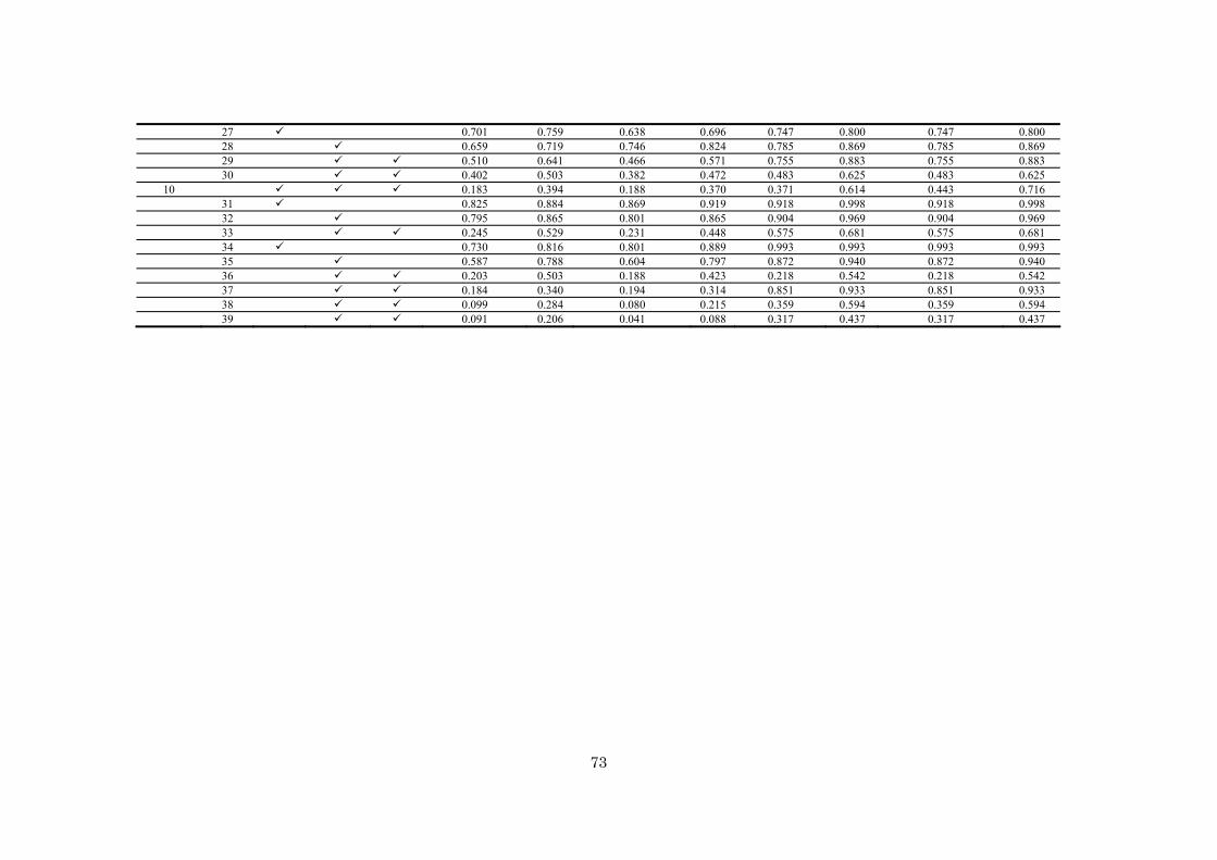
73

27 0.701 0.759 0.638 0.696 0.747 0.800 0.747 0.800 28 0.659 0.719 0.746 0.824 0.785 0.869 0.785 0.869 29 0.510 0.641 0.466 0.571 0.755 0.883 0.755 0.883 30 0.402 0.503 0.382 0.472 0.483 0.625 0.483 0.625

10 0.183 0.394 0.188 0.370 0.371 0.614 0.443 0.716 31 0.825 0.884 0.869 0.919 0.918 0.998 0.918 0.998 32 0.795 0.865 0.801 0.865 0.904 0.969 0.904 0.969 33 0.245 0.529 0.231 0.448 0.575 0.681 0.575 0.681 34 0.730 0.816 0.801 0.889 0.993 0.993 0.993 0.993 35 0.587 0.788 0.604 0.797 0.872 0.940 0.872 0.940 36 0.203 0.503 0.188 0.423 0.218 0.542 0.218 0.542 37 0.184 0.340 0.194 0.314 0.851 0.933 0.851 0.933 38 0.099 0.284 0.080 0.215 0.359 0.594 0.359 0.594 39 0.091 0.206 0.041 0.088 0.317 0.437 0.317 0.437