cap budgeting theses.2
TRANSCRIPT

Industrial and Financial Economics Master Thesis No 2002:38
Capital Budgeting Sophistication and Performance
- A Puzzling Relationship
Helen Axelsson, Julija Jakovicka & Mimmi Kheddache

Graduate Business School School of Economics and Commercial Law Göteborg University ISSN 1403-851X Printed by Elanders Novum

III
ABSTRACT This thesis investigates the relationship between capital budgeting sophistication and firm performance. Initially, the theoretical relationship is analysed. The traditional financial view, predicting a positive relationship, is presented as a starting point for the analysis. Other aspects, based on contingency and behavioural theories, are then brought into the discussion. These aspects shed light on the complexity of the relationship and question the positive relationship advocated by traditional financial theory. In a second step, a model is constructed in order to measure the relationship between capital budgeting sophistication and performance empirically. The statistical model used is the regression analysis. Based on theory, variables for capital budgeting sophistication, and performance are constructed. Moreover, relevant explanatory variables are defined. Three different definitions of capital budgeting sophistication, ranging from simple to more complex, are used in order to be able to measure whether the choice of variable affects the findings. For the same reason three different performance measures are used. The final step of this thesis is to test the model constructed empirically on the Swedish market. Due to insufficient data the model is only partially tested. The results obtained are mostly negative and insignificant. These findings do not support traditional financial theory. Key words: Capital Budgeting, Capital Budgeting Sophistication, Performance, Investment Decisions, Investment Appraisal, Net Present Value, Internal Rate of Return, Accounting Rate of Return, Payback Period.

IV
ACKNOWLEDGEMENTS The completion of this thesis has been possible thanks to a number of people. First of all, we would like to acknowledge our gratitude to PhD Gert Sandahl, who has invested a lot of time and effort in supporting us throughout the thesis work. His brilliant suggestions and ideas have been of the greatest importance to this thesis. We would also like to thank PhD Stefan Sjögren for providing essential comments and bringing us down to earth when our intentions were over-ambitious. Many thanks to both PhD Gert Sandahl and PhD Stefan Sjögren for offering us the opportunity to use data from one of their surveys concerning capital budgeting practices. Without this information the accomplishment of the thesis would not have been possible. Moreover, we are very grateful to Professor Lennart Flood for his insightful help in econometric issues. We would also like to express our gratitude to the people at the Department of Industrial and Financial Economics who took their time to comment on our questionnaire before it was finally sent out. Finally, we would like to express our thanks to all those academics, who answered the questionnaire and thereby helped us with the completion of this thesis. Thanks to all of you for your help! Göteborg, January 2003 Helen Axelsson Julija Jakovicka Mimmi Kheddache
V
TABLE OF CONTENTS 1. INTRODUCTION .......................................................................................................... 1
1.1 BACKGROUND .............................................................................................1 1.2 PROBLEM DISCUSSION.................................................................................2 1.3 PURPOSE......................................................................................................8 1.4 POTENTIAL CONTRIBUTION OF THE STUDY..................................................9
2. GENERAL METHODOLOGY ................................................................................ 11
2.1 PROCESS DESCRIPTION ..............................................................................11 2.2 STATISTICAL APPROACH ...........................................................................12
2.2.1 Correlation Analysis ..........................................................................13 2.2.2 Matched Pairs Approach....................................................................14 2.2.3 Regression Analysis...........................................................................14 2.2.4 Choice of Model ................................................................................17 3. VARIABLES– THEORETICAL FRAMEWORK AND PREVIOUS
RESEARCH........................................................................................................................ 19
3.1 CAPITAL BUDGETING SOPHISTICATION .....................................................19 3.1.1 The Choice of Capital Budgeting Techniques...................................19 3.1.2 The Application of Sophisticated Capital Budgeting Techniques.....21 3.1.3 The Capital Budgeting Process..........................................................26 3.1.4 Behavioural Perspective of Capital Budgeting..................................34
3.2 PERFORMANCE ..........................................................................................35 3.2.1 Market Performance...........................................................................36 3.2.2 Accounting Performance ...................................................................38 3.2.3 Tobin’s q ............................................................................................44
3.3 EXPLANATORY VARIABLES........................................................................45 3.3.1 Size.....................................................................................................46 3.3.2 Capital Intensity .................................................................................51 3.3.3 Degree of Risk ...................................................................................53 3.3.4 Degree of Diversification...................................................................56 3.3.5 Leverage.............................................................................................60 3.3.6 Industry Characteristics .....................................................................63
4. GENERAL MODEL.................................................................................................... 65
4.1 CAPITAL BUDGETING SOPHISTICATION (CBS) ..........................................65 4.1.1 CBS Definition I ................................................................................66 4.1.2 CBS Definition II ...............................................................................67 4.1.3 CBS Definition III..............................................................................70
4.2 PERFORMANCE ..........................................................................................72 4.2.1 Market Performance...........................................................................72 4.2.2 Accounting Performance ...................................................................72

VI
4.2.3 Tobin’s q ............................................................................................73 4.3 EXPLANATORY VARIABLES .......................................................................74
4.3.1 Size .....................................................................................................74 4.3.2 Capital Intensity .................................................................................75 4.3.3 Degree of Risk....................................................................................75 4.3.4 Diversification....................................................................................76 4.3.5 Leverage .............................................................................................77 4.3.6 Industry Characteristics......................................................................77
4.4 COMPREHENSIVE DESCRIPTION OF GENERAL MODEL................................78 4.4.1 Quality of General Model – Validity and Practicality .......................81
5. DATA .............................................................................................................................. 85
5.1 DATA FOR DEFINING CAPITAL BUDGETING SOPHISTICATION ....................85 5.1.1 Survey by Sandahl & Sjögren ............................................................85 5.1.2 Survey by Axelsson, Jakovicka & Kheddache ..................................87
5.2 ACADEMICS’ VIEW OF CAPITAL BUDGETING SOPHISTICATION..................90 5.3 DATA FOR DEFINING THE PERFORMANCE VARIABLE AND THE EXPLANATORY VARIABLES .............................................................................94 5.4 RELIABILITY ..............................................................................................95 5.5 DATA QUALITY’S EFFECT ON THE VALIDITY OF THE MODEL FOR EMPIRICAL TESTS ............................................................................................96 5.6 SUMMARY – MODEL FOR EMPIRICAL TESTS ............................................101
6. EMPIRICAL TESTS ON THE SWEDISH MARKET .................................... 105
6.1 PRESENTATION OF EMPIRICAL RESULTS ..................................................105 6.1.1 Model I .............................................................................................105 6.1.2 Model II............................................................................................114
6.2 ANALYSIS OF EMPIRICAL RESULTS ..........................................................118 6.2.1 The Relationship between Capital Budgeting Sophistication and Performance...............................................................................................118 6.2.2 Different Definitions’ Effect on Results ..........................................123 6.2.3 The Relationship between Explanatory Variables and the Main Variables....................................................................................................124
7. CONCLUSIONS ........................................................................................................ 131
8. SUGGESTIONS FOR FURTHER RESEARCH............................................... 135
BIBLIOGRAPHY........................................................................................................... 137
APPENDIX I ......................................................................................................................... I
APPENDIX II .................................................................................................................... III
APPENDIX III.................................................................................................................... V
APPENDIX IV................................................................................................................... VI
APPENDIX V ................................................................................................................. VIII

VII
APPENDIX VI...................................................................................................................XI
APPENDIX VII ............................................................................................................... XV
APPENDIX VIII.............................................................................................................. XX
APPENDIX IX............................................................................................................. XXIII

VIII
EQUATIONS Equation 1 The Weighted Average Cost of Capital (WACC).....................................24 Equation 2 Return on Assets (ROA) ...........................................................................39 Equation 3 Return on Equity (ROE)............................................................................40 Equation 4 Covariance.................................................................................................55 Equation 5 CBS Variable, Definition I........................................................................67 Equation 6 CBS Variable, Definition II ......................................................................68 Equation 7 Scaling Factor, CBS Variable Definition II ..............................................68 Equation 8 CBS Variable, Definition III .....................................................................71 Equation 9 Market Performance (∆MV) .....................................................................72 Equation 10 Operating Rate of Return (ORR) ............................................................72 Equation 11 Tobin’s q..................................................................................................73 Equation 12 Industry Adjusted Market Performance (∆MVAdj)..................................77 Equation 13 Industry Adjusted Operating Rate of Return (ORRAdj)...........................78 Equation 14 Industry Adjusted Tobin’s q (qAdj) ..........................................................78 Equation 15 Regression Equation – CBS Definition I, ORRAdj...................................80 Equation 16 Regression Equation – CBS Definition I, qAdj.........................................80 Equation 17 Regression Equation – CBS Definition I, ∆MVAdj ..................................80 Equation 18 Regression Equation – CBS Definition II, ORRAdj .................................80 Equation 19 Regression Equation – CBS Definition II, qAdj .......................................80 Equation 20 Regression Equation – CBS Definition II, ∆MVAdj .................................80 Equation 21 Regression Equation – CBS Definition III, ORRAdj ................................81 Equation 22 Regression Equation – CBS Definition III, qAdj ......................................81 Equation 23 Regression Equation – CBS Definition III, ∆MVAdj................................81 Equation 24 Model I for Empirical Test - Large Sample ..........................................103 Equation 25 Model I for Empirical Test - Small Sample ..........................................103 Equation 26 Model II for Empirical Test - Large Sample.........................................103 Equation 27 Model II for Empirical Test - Small Sample.........................................104 Equation 28 Regression Equation – Large Sample, Model I, Dummies...................106 Equation 29 Regression Equation - Small Sample, Model I, Dummies, ORRAdj ......109 Equation 30 Regression Equation - Small Sample, Model I, Dummies, ∆MVAdj......109 Equation 31 The Goldfeld-Quandt Test Statistic ......................................................XV Equation 32 Errors of the Linear Regression Model ............................................... XVI Equation 33 The Durbin-Watson Test Statistic ....................................................... XVI Equation 34 The Jarque-Bera Test Statistic...........................................................XVIII Equation 35 The t-test Statistic..............................................................................XVIII Equation 36 The F-test Statistic............................................................................... XIX
IX
FIGURES AND TABLES Figure 1 Disposition of the Thesis .............................................................................. 12 Figure 2 Illustration of Firm and Project Risk ............................................................ 25 Figure 3 Long Run Average Cost (LAC) Curve......................................................... 47 Figure 4 Performance (ROA) and Size ....................................................................... 49 Figure 5 Optimal Leverage ......................................................................................... 61 Figure 6 Calculation of wi and the Scaling Factor αjk ................................................. 69 Figure 7 Average score – Capital Budgeting Techniques........................................... 90 Figure 8 Average Score – Application of Capital Budgeting Techniques.................. 91 Figure 9 Average Score – Issues Related to WACC................................................... 92 Figure 10 Average Scores – Capital Budgeting Process............................................. 93 Figure 11 NPV – Distribution Sophistication Scores .................................................XI Figure 12 IRR –Distribution Sophistication Scores....................................................XI Figure 13 DPB – Distribution Sophistication Scores.................................................XII Figure 14 ARR – Distribution Sophistication Scores ................................................XII Figure 15 PB – Distribution Sophistication Scores.................................................. XIII Figure 16 Determination of the Discount Rate ........................................................ XIII Figure 17 Stages in the Capital Budgeting Process .................................................XIV Table 1 Estimated Regression Coefficients - Large Sample, Model I...................... 105 Table 2 Estimated Regression Coefficients - Large Sample, Model I, Dummies .... 107 Table 3 Estimated Regression Coefficients - Small Sample, Model I...................... 112 Table 4 Estimated Regression Coefficients - Small Sample, Model I, Dummies .... 113 Table 5 Estimated Regression Coefficients - Large Sample, Model II .................... 114 Table 6 Estimated Regression Coefficients - Small Sample, Model II .................... 117 Table 7 Correlation Matrix – Large Sample, Model I .............................................. XX Table 8 Correlation Matrix – Small Sample, Model I, 1997-1999 ..........................XXI Table 9 Correlation Matrix – Small Sample, Model I, Remaining Years ..............XXII Table 10 Tests of Regression Assumptions - Large Sample................................. XXIII


CAPITAL BUDGETING SOPHISTICATION AND PERFORMANCE CHAPTER 1
1
1. INTRODUCTION
1.1 Background
n efficient economic system calls for a dependable mechanism to allocate its resources. Christy (1966) describes that land, labour and capital are to
be directed to their best uses, and should hence be placed in the hands of those who can use them most capably. In a market economy, this allocation process consists largely of a set of private decisions, which are directed by a network of free markets and flexible prices (Ibid). Important among these decisions are capital investments decisions that according to Northcott (1995) are vital at two levels: for the future operability of the individual firm making the investment, and for the economy of the nation as a whole. At the firm level, capital investment decisions have implications for many aspects of operations, and often exert a crucial impact on survival, profitability and growth. At the national level, the proper planning and allocation of capital investment are essential to an efficient utilisation of other resources, poorly placed investment reduces the productivity of labour and materials and sets a lower ceiling on the economy’s potential output. With this in mind it is no wonder that capital investment or capital budgeting is a central application of financial theory taught at business schools. Also during our studies at the School of Economics and Commercial Law at Göteborg University, the advantages and applications of sophisticated capital budgeting procedures based on cash flows, risk and the time value of money have been taught. The advantage of applying such procedures is however generally taken for granted and seldom questioned. Theoretically sophisticated procedures are seen as tools for maximising shareholders’ wealth, which is the same as maximising the value of the firm (Copeland & Weston, 1992). This fact is often approximated to the relationship that firms using more sophisticated capital budgeting procedures should be able to perform better over time (Christy, 1966; Klammer, 1973). Empirical studies concerning the adoption of sophisticated capital budgeting procedures have shown that even though the degree of adoption has increased over time, there is an obvious “theory-practice gap” (Klammer, 1972; Schall, Sundem & Geijsbeek, 1978; and Graham & Harvey, 2001). This raises the question why firms do not adopt
A

CAPITAL BUDGETING SOPHISTICATION AND PERFORMANCE CHAPTER 1
2
sophisticated capital budgeting procedures, although it is assumed to result in improved performance. Does the theoretical relationship not hold empirically? This is a question, which we found very interesting to develop and analyse more thoroughly. A number of articles, linking capital budgeting sophistication and performance, have further inspired us when choosing this subject for our thesis.
1.2 Problem Discussion According to financial theory, the objective of the firm is to maximise the wealth of its shareholders. The optimal investment decision is hence the one that maximises the present value of shareholders’ wealth (Copeland & Weston, 1992). Sophisticated capital budgeting procedures can under the assumption of economic rationality all be regarded as means, which a firm uses in order to fulfil its objective, i.e., to maximise shareholders’ wealth (Ibid). This fact indicates that firms can increase or even maximise its shareholder wealth by using sophisticated capital budgeting procedures. Hence, from a perspective of traditional financial theory, the relationship between capital budgeting sophistication and performance is expected to be positive. Earlier studies on the relationship between capital budgeting sophistication and performance have presented limited reasoning about the foundations of this assumption and have to a great extent seen it as a matter of course. However, there are also contrary arguments, indicating that the relationship is far more complex. One argument is that the implementation of sophisticated capital budgeting techniques can be regarded as a means of coping with acute resource scarcity. This is referred to as the economic stress hypothesis and implies that the application of sophisticated capital budgeting techniques is more often associated with a poor financial performance (Haka, Gordon & Pinches, 1985). Some researchers emphasise contingency theory and argue that it is not the implementation of sophisticated procedures that is important, but the fit between the procedures and the firm context. Important issues to consider are organisational structure, financial status, management style and reward system (Pike, 1986; Haka et al, 1985; Pinches, 1982). Further, it has been pointed out that the degree of environmental uncertainty may influence the benefits that a firm has from implementing or improving sophisticated capital budgeting procedures.

CAPITAL BUDGETING SOPHISTICATION AND PERFORMANCE CHAPTER 1
3
These arguments indicate that the perspective of traditional financial theory can be questioned. The theoretical relationship is very complex and could be analysed more in-depth. This reasoning naturally leads on to the first problem of this thesis: How can the relationship between capital budgeting sophistication and
performance be described from a theoretical perspective? The conflicting theoretical arguments as well as the increased practical application of sophisticated capital budgeting procedures, starting in the 1950s and 1960s, have caught the interest of some researchers, who have tried to measure the relationship quantitatively (Christy, 1966; Klammer, 1973; Kim, 1982; Pike, 1984; Haka et al, 1985; Farragher, Kleiman & Sahu, 2001). When trying to estimate a complex relationship in quantitative terms a key issue is to find an appropriate statistical model that captures the relationship most accurately. The underlying assumptions, as well as the advantages and the disadvantages of alternative models, have to be considered in the light of the purpose of the survey. Generally, there is a trade-off between analysing firm specific factors in-depth and including a large number of companies. The choice influences the possibility to generalise the findings. In this specific case there are a number of measures of association, and it is not obvious which measure or model best describes the relationship. In earlier studies three different measures of association have been used, i.e., simple correlation analysis, matched pairs approach and multiple regression analysis. Irrespective of what kind of statistical model is used, the main variables, capital budgeting sophistication and firm performance, have to be defined and quantified. In capital budgeting literature, two main approaches defining capital budgeting can be distinguished: the normative approach and the process approach. The normative approach, which represents traditional capital budgeting theory, presents rules for how firms should treat investment decisions. The main emphasis is generally put on the financial evaluation and selection of proposed investments in long-term assets. The development of advanced capital budgeting techniques and their application in various situations are hence key issues. Capital budgeting techniques are generally categorized as either sophisticated or naive (Pinches, 1994). Gordon & Pinches

CAPITAL BUDGETING SOPHISTICATION AND PERFORMANCE CHAPTER 1
4
(1984, p.1, quoted by Myers, Gordon & Hamer, 1991) describe this categorization:
“Capital budgeting approaches that consider risk and the discounted cash flow stream associated with a project are often referred to as sophisticated methods. These methods also assume that capital budgeting decision makers act in a rational manner. In contrast, capital budgeting approaches that do not consider the time value of money and/or risk of a project are often referred to as naive methods.”1
The two most popular naive techniques are the payback period (PB) and the accounting rate of return (ARR), while the most popular sophisticated techniques are the net present value (NPV) and the internal rate of return (IRR) (Pike & Neale, 1999; Copeland & Weston, 1992). In addition to these techniques there are a number of variations such as discounted payback (DPB) and the newer concepts of real options and value based measures (Northcott, 1995; Copeland & Weston, 1992). Process approaches to capital budgeting take a broader perspective and try to explain how firms treat investment decisions in practice, i.e., how projects become identified, developed, justified and finally approved. Based on studies conducted by Aharoni (1966), Bower (1970) and King (1975) the capital budgeting process is generally described as a many-sided activity, including a number of distinct stages. When analysing the definitions used in previous studies treating the relationship in question, one can observe an obvious chronological pattern. In the early studies performed by Christy (1966) and Klammer (1973) the definition of capital budgeting sophistication is rather narrow and focuses merely on the use of theoretically superior methods for financial evaluation. In the 1960s and 1970s, when the surveys were performed, this focus was natural since the academic literature also emphasised the financial evaluation. In later studies the definition is gradually broadening and becoming closer to the process oriented view, which considers the whole capital budgeting process. Kim (1982) interpreted the capital budgeting decision as a system of 1 Gordon & Pinches 1984, Improving Capital Budgeting: A Decision Support System, Reading, MA: Addison-Weasley, p.1, mentioned in Myers, Gordon & Hamer, 1991, p.324.

CAPITAL BUDGETING SOPHISTICATION AND PERFORMANCE CHAPTER 1
5
interrelated components and defined sophistication as being determined by the existence of nine activities. Kim’s definition is further developed by Pike (1984) and Farragher et al (2001), whose definitions are more detailed. One can hence conclude that the definitions used in previous studies have become broader and increasingly more detailed over time. The main problem arising from the increasingly broader definitions is the great range of issues that have to be taken into consideration. In some cases a simple definition might be more striking than a very complex one. Therefore, it may be essential to limit the number of components and put emphasis on including the right components rather than a great number of components. The second crucial variable is performance. Performance can in this context be defined as a measure of value generation. Generally, performance measures can be calculated using two different spheres, the accounting sphere and the economic sphere. Measuring corporate performance applying the economic sphere implies using information based on the firm’s stock performance. The accounting sphere, on the other hand, includes measures derived from financial statements. In previous studies on the relationship between capital budgeting sophistication and performance either accounting data or stock market values have been used in order to measure firm performance. It is difficult to conclude that one way to measure performance is better than the other. Reasons and justifications for applying measures from one of the two alternative spheres can be found in almost all earlier studies. As discussed initially, financial theory indicates that the main reason for implementing sophisticated capital budgeting procedures is to maximise, or at least increase, shareholders’ wealth. In the same way as an individual maximises the expected satisfaction gained from consumption over time by choosing the optimal investment decision, the objective of a firm is to maximize the present value of shareholders’ lifetime consumption. That is equal to maximizing the price per share of stock (Copeland, 1979). Using this reasoning it might seem most appropriate to measure performance by using market information (Haka et al, 1985). The fact that it is probably difficult for market participants to acquire information about changes in capital budgeting policy and whether sophisticated capital budgeting techniques are properly
CAPITAL BUDGETING SOPHISTICATION AND PERFORMANCE CHAPTER 1
6
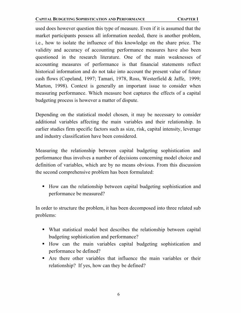
used does however question this type of measure. Even if it is assumed that the market participants possess all information needed, there is another problem, i.e., how to isolate the influence of this knowledge on the share price. The validity and accuracy of accounting performance measures have also been questioned in the research literature. One of the main weaknesses of accounting measures of performance is that financial statements reflect historical information and do not take into account the present value of future cash flows (Copeland, 1997; Tamari, 1978, Ross, Westerfield & Jaffe, 1999; Marton, 1998). Context is generally an important issue to consider when measuring performance. Which measure best captures the effects of a capital budgeting process is however a matter of dispute. Depending on the statistical model chosen, it may be necessary to consider additional variables affecting the main variables and their relationship. In earlier studies firm specific factors such as size, risk, capital intensity, leverage and industry classification have been considered. Measuring the relationship between capital budgeting sophistication and performance thus involves a number of decisions concerning model choice and definition of variables, which are by no means obvious. From this discussion the second comprehensive problem has been formulated: How can the relationship between capital budgeting sophistication and
performance be measured? In order to structure the problem, it has been decomposed into three related sub problems: What statistical model best describes the relationship between capital
budgeting sophistication and performance? How can the main variables capital budgeting sophistication and
performance be defined? Are there other variables that influence the main variables or their
relationship? If yes, how can they be defined?

CAPITAL BUDGETING SOPHISTICATION AND PERFORMANCE CHAPTER 1
7
When a way of measuring the relationship has been developed, the natural continuation is to estimate the relationship empirically. A number of studies analysed the empirical effect of applied capital budgeting activities on firms’ performance. Christy (1966), Klammer (1973), Kim (1982), Haka et al (1985) and Farragher et al (2001) have performed empirical studies including American firms, and Pike (1984) has performed a similar survey on a sample consisting of British firms. On the Swedish market Renck (1966), Tell (1978) and Yard (1987) have mapped investment practice among Swedish firms, but no study concerning the relationship with performance has been made. An interesting issue would hence be to perform an empirical survey on the Swedish market. The surveys performed on the American and British markets give mixed results. Christy (1966), Klammer (1972), Pike (1984), Haka et al (1985) and Farragher et al (2001) found a negative relationship between capital budgeting sophistication and performance, which in most cases was insignificant. Only Kim established a significant positive relationship in his survey from 1982. As mentioned before, the definitions used in the studies differ and have developed from being very simple to becoming increasingly more complex. It would hence be interesting to analyse whether this development of the definitions has influenced the empirical results obtained. Making a very rough comparison of the surveys one cannot discern any large differences in the results obtained, even though the definitions used have become increasingly more detailed. It is however, not possible to make a correct and fair comparison, since the studies involved different samples and have been performed at different points in time. In order for a correct comparison to be possible, a survey including several definitions would be necessary. This discussion leads on to the third and last problem to be treated in this thesis: What is the empirical relationship between capital budgeting and
performance within firms on the Swedish market?

CAPITAL BUDGETING SOPHISTICATION AND PERFORMANCE CHAPTER 1
8
The empirical test gives us the opportunity to investigate the following sub problem: How does the definition of the main variables, capital budgeting
sophistication and performance, influence the results obtained? The three comprehensive problems and their sub problems raised in the problem discussion leads to the purpose of this thesis.
1.3 Purpose The purpose of this thesis consists of three main purposes and a number of sub purposes that are presented below.
1. To describe the relationship between capital budgeting sophistication and performance from a theoretical point of view.
2. To analyse how the relationship between capital budgeting
sophistication and performance can be measured. a. To identify a working statistical model for measuring the
relationship between capital budgeting sophistication and performance.
b. To define the main variables capital budgeting sophistication and performance.
c. To identify and define variables that may influence the main variables or their relationship.
3. To test the relationship empirically using data from the Swedish market,
on the assumption that accessible data allows such a test. a. To analyse the empirical results obtained. b. To analyse how the definition of the main variables, capital
budgeting sophistication and performance, affects the empirical results.

CAPITAL BUDGETING SOPHISTICATION AND PERFORMANCE CHAPTER 1
9
1.4 Potential Contribution of the Study Our aim is to construct a model that enables the comparison of how different definitions of the main variables influence the empirical results. This has not been considered in earlier studies and can be regarded as a main contribution of this thesis. Moreover, no study of this kind treating Swedish firms has been undertaken before. Therefore, the findings of this study aim at creating knowledge of empirical evidence of the relationship between capital budgeting sophistication and performance in Sweden.


CAPITAL BUDGETING SOPHISTICATION AND PERFORMANCE CHAPTER 2
11
2. GENERAL METHODOLOGY
he main concerns of this thesis are to establish the relationship between capital budgeting sophistication and performance from a theoretical point
of view, to create a model in order to measure this relationship, and finally to test the relationship using data from the Swedish market. This chapter constitutes a description of the methodological approach used when dealing with these concerns2.
2.1 Process Description An extensive literature review using external secondary data was performed at the initial stage of the thesis writing in order to gain general, as well as specific, knowledge about the subject. External secondary data includes, for example, periodicals, theses and other literature dealing with the particular research field (Thiétart, 2001). By analysing general literature and previous studies on the subject, an understanding of the relationship was created. More specific literature treating capital budgeting sophistication and corporate performance was also studied in order to gain a deeper knowledge about these variables and their characteristics. Mainly, the library databases GUNDA and LIBRIS were used in order to search for books available within the Nordic countries. When searching for articles we primarily used full-text databases such as Jstor and Science Direct Elsevier as well as Artikelsök, which all include a large number of academic journals, and can be considered to be of high reliability. The search process was very broad to begin with but gradually became narrower as suitable search words were found. The search words used are listed in Appendix III. The external secondary data review helped us to map and analyse the theoretical relationships and constituted a basis for defining the main variables and other variables affecting the relationship between capital budgeting sophistication and performance. This theoretical analysis is presented in Chapter 3. The analysis resulted in the construction of a model, which is presented in Chapter 4. In Chapter 5, the data used in order to quantify the
2 Further methodological concerns will be discussed in Chapter 5.
T
CAPITAL BUDGETING SOPHISTICATION AND PERFORMANCE CHAPTER 2
12
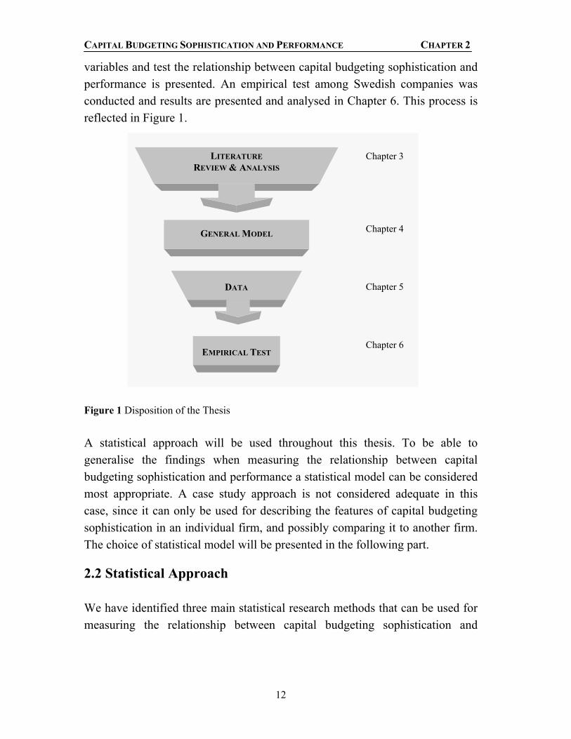
variables and test the relationship between capital budgeting sophistication and performance is presented. An empirical test among Swedish companies was conducted and results are presented and analysed in Chapter 6. This process is reflected in Figure 1.
Figure 1 Disposition of the Thesis A statistical approach will be used throughout this thesis. To be able to generalise the findings when measuring the relationship between capital budgeting sophistication and performance a statistical model can be considered most appropriate. A case study approach is not considered adequate in this case, since it can only be used for describing the features of capital budgeting sophistication in an individual firm, and possibly comparing it to another firm. The choice of statistical model will be presented in the following part.
2.2 Statistical Approach We have identified three main statistical research methods that can be used for measuring the relationship between capital budgeting sophistication and
LITERATURE REVIEW & ANALYSIS
GENERAL MODEL
DATA
EMPIRICAL TEST
Chapter 3
Chapter 4
Chapter 5
Chapter 6

CAPITAL BUDGETING SOPHISTICATION AND PERFORMANCE CHAPTER 2
13
corporate performance: pairwise correlation analysis, matched pairs approach3 and regression analysis. Correlation analysis involves the construction of correlation matrices with different variables. Among earlier studies measuring the relationship in question this method is employed by Christy (1966) and partly by Pike (1984). Regression analysis is the most commonly used method for measuring the relationship in consideration (Klammer, 1973; Kim, 1982; Pike, 1984; Farragher et al, 2001), while the matched pairs approach is applied in relatively few articles (Haka et al, 1985; Myers et al, 1991). The three alternative research methods are accounted for in this chapter. 2.2.1 Correlation Analysis Correlation analysis is used in relatively few articles, e.g.,, Christy (1966). However, this type of analysis is, to a larger extent, applied as a part of the research methodology, e.g.,, Pike (1984). The correlation between two variables measures the degree of linear association between them (Hill et al, 2001). Correlation may vary between –1 and 1, where the former indicates a perfect negative (inverse) relationship and the latter signifies a perfect positive (direct) relationship. A value of zero indicates that there is no linear relationship between the two variables. The magnitude of the absolute value of correlation shows “the strength” of the linear association, the closer it is to 1, the more it approaches the exact linear association (Ibid). The pairwise correlation between various variables can be summarised in a correlation matrix. The correlation matrices employed in the studies often serve two purposes. Firstly, to investigate the pairwise relationships between different variables, and secondly, to ascertain that the underlying linear regression assumption of collinearity is not violated (Pike, 1984). It is important to stress that the correlation analysis only considers the relationship between pairs of variables (pairwise association), thereby implying that the influence of other variables on the relationship cannot be examined.
3 Also referred to as “matched-pair experimental design” by Myers et al (1991).

CAPITAL BUDGETING SOPHISTICATION AND PERFORMANCE CHAPTER 2
14
2.2.2 Matched Pairs Approach Matched pairs approach implies comparing the performance of a number of experimental firms, using sophisticated capital budgeting techniques, with the performance of matched control firms, using naive capital budgeting techniques. In order to ensure the closest match between the control firms and experimental firms, the control firms are matched on the basis of various factors such as industry, size, risk and Tobin’s q (Haka et al, 1985; Myers et al, 1991). In these studies performance is compared over a period of time, in which the experimental firms have switched from naive to sophisticated capital budgeting techniques. The matched pairs approach aims at evaluating the economic consequences of a change in capital budgeting techniques in the experimental firms. This means that, employed to examine whether the performance of the experimental firms change after the implementation of sophisticated capital budgeting techniques compared to the performance of the control firms for the same period. Matching for such variables as size, risk and industry makes it possible to examine the relationship between capital budgeting sophistication and performance in isolation, i.e., keeping the influence of these variables constant. 2.2.3 Regression Analysis Regression analysis is the most commonly used method for measuring the association between the degree of capital budgeting sophistication and corporate performance. It involves estimating a regression model that enables the researcher to measure the relationship in consideration. The model is set up because it is believed that there is a linear relationship between one dependent and one or a number of independent variables. For the capital budgeting area the regression model can be constructed using a certain measure of corporate performance as the dependent variable and the degree of capital budgeting sophistication as one of the independent variables. A regression model employing only one independent variable is referred to as a simple linear regression model. A simple regression model has been used by Kim (1982). However, the majority of the articles employ a multiple regression analysis as a research method for the relationship in consideration (Klammer, 1973, Pike, 1984, Farragher et al, 2001). When applying the multiple regression other independent variables are also assumed to have some kind of linear relationship

CAPITAL BUDGETING SOPHISTICATION AND PERFORMANCE CHAPTER 2
15
with corporate performance. By including these variables in a regression model, one aims to isolate their effect on the relationship between capital budgeting sophistication and performance. Dependent and independent variables and their definitions determine the functional form of the model. In the choice of model, economic principles and logical reasoning play a vital role by examining what variables are likely to influence the dependent variable and how the dependent variable is believed to respond when these variables change (Hill, Griffiths & Jugde, 2001). The regression model assumes a linear functional form of the relationship, i.e., that there will be a linear relationship between independent variables and a dependent variable. However, it is important to note that linearity refers to the manner in which the parameters enter the equation, not necessarily to the relationship between variables (Greene, 1997). One should also consider that a major objective of choosing the functional form is to create a model, which fulfils the assumptions of the regression model. These assumptions are the conditions under which it is appropriate to use a regression for analysis. If the assumptions are not valid, then the estimated regression coefficients will not be the best linear unbiased estimators (Hill et al, 2001)4. The assumptions of the linear regression model are as follows (Ibid):
1. y = β1 + β2xt2 + … + βKxtK + et, t = 1,…, T. Assumption of linearity. 2. E(yt) = β1 + β2xt2 + … + βKxtK ⇔ E[et] = 0. The expected (average)
value of yt depends on the values of the explanatory variables and the unknown parameters. This is equivalent to assumption that each random error has a probability distribution with a mean equal to zero.
3. var(yt) = var(et) = σ2. The variance of the probability distribution of yt does not change with each observation. It is equal to the variance of the probability distribution of the random error, σ2, implying that the errors are homoskedastic.
4. cov (yt, ys) = cov (et, es) = 0. The covariance between two observations of the dependent variables as well as between two random errors is zero.
4 For a discussion on the Best Linear Unbiased Estimators (BLUE) see Hill et al (2001) p. 77-79.

CAPITAL BUDGETING SOPHISTICATION AND PERFORMANCE CHAPTER 2
16
5. The values of the explanatory variables (xtk) are not random and are not exact linear functions of other explanatory variables. The violation of the latter assumption is called exact collinearity.
6. yt ~ N(β1 + β2xt2 + … + βKxtK, σ2) ⇔ et ~ N(0, σ2). The values of yt are normally distributed around their mean, which is equivalent to assuming that random errors are normally distributed. This assumption is optional.
Tests of the Multiple Regression Model5 Since fulfilling the assumption of the regression model is of great importance, tests need to be conducted to make sure that these assumptions are valid. Testing the assumptions is sometimes a difficult task, since economic data is not obtained by a controlled laboratory experiment and is often “messy” (Hill et al, 2001). Moreover, some assumptions cannot be tested. Assumption 1 is a general assumption of linearity and is difficult to test. Assumption 2 is a theoretical assumption and cannot be tested. Assumption 3 can be tested using the Goldfeld-Quandt test. Assumption 4 can be tested by performing the Durbin-Watson test . Assumption 5 can be tested using correlation analysis and “auxiliary”
regressions. Assumption 6 can be tested by estimating whether residuals are normally
distributed and can be accomplished with the Jarque-Bera test. As mentioned above, a multiple regression is set up because there is a belief that all the explanatory variables influence the dependent variable. It must then be examined whether the data provide any evidence to support this belief. Firstly, in order to find out whether the dependent variable is related to any single explanatory variable, the “test of significance”, t-test, can be used. Secondly, if the overall significance of a model is being tested in the multiple regression model, the F-test should be used to jointly test the relevance of all the included explanatory variables.
5 The description of tests and their application is provided in Appendix VII.

CAPITAL BUDGETING SOPHISTICATION AND PERFORMANCE CHAPTER 2
17
2.2.4 Choice of Model All three models discussed above have their weaknesses and strengths. One of the drawbacks of the correlation analysis is that it only shows the pairwise association between two variables, hence, the effect that other factors might have on this association cannot be estimated and isolated. The matched pairs approach takes into account the fact that firm specific factors have to be approximated in order to evaluate whether a firm can improve its performance by switching from naive to sophisticated capital budgeting techniques. The ideal test would be to compare a firm’s performance over a time period when it uses sophisticated techniques with its performance over the same period of time while it uses naive techniques. Since this is not possible the second best alternative is to compare a firm that has switched from a naive to a sophisticated technique (experimental firm) with a firm using either naive or sophistication technique (control firm), over the same period of time. The matched pairs approach allows to design a sample of control firms so that the control firm’s characteristics, e.g.,, industry, size, risk, match those of the experimental firm at most. This model will however put a limit to the number of firms included in the study. To find suitable experimental firms and match these with a number of control firms demands a great effort and, hence, the number of experimental firms must be limited. A limited number of observations can have a negative effect on the degrees of freedom in the hypothesis testing, and hence on the reliability of the results. The regression analysis allows for a larger number of firms to be included in the analysis. Firm-specific factors can in this case be taken into account by including additional independent variables in the multiple regression model. However, a large number of observations can sometimes be an obstacle for performing a deep investigation into firm specific factors. Besides, the number of additional independent variables controlling for firm-specific factors cannot be increased continuously due to high inter-correlation between the variables (Pike, 1984). In contrast, the possibilities of controlling for the firm-specific variables are less limited when using the matched pairs approach. Another caveat in the regression methodology is that the regression model assumes a linear relationship between the independent and the dependent variables when

CAPITAL BUDGETING SOPHISTICATION AND PERFORMANCE CHAPTER 2
18
in reality this relationship might be non-linear (Kim, 1982). The latter obstacle can, however, be overcome to a large extent by performing transformations of the independent variables. We consider the multiple regression analysis to be the most appropriate research method in our case. Firstly, the multiple regression method allows us to include a larger number of observations in the analysis and thereby provides a possibility to generalise the findings. Secondly, just as the matched pair approach, the regression analysis allows taking into consideration other factors that may influence the relationship between capital budgeting sophistication and performance. Finally, as mentioned above, the matched pairs approach is generally employed in order to examine the economic effects of a change in the capital budgeting techniques. It would be very time consuming to find a sample of firms for which the time of implementation of a sophisticated capital budgeting technique is known and moreover to find matching control firms. Under present conditions it appears to be more realistic to gather information and perform a regression analysis by accurate means.

CAPITAL BUDGETING SOPHISTICATION AND PERFORMANCE CHAPTER 3
19
3. VARIABLES– THEORETICAL FRAMEWORK AND
PREVIOUS RESEARCH
o be able to apply the chosen statistical model, the variables capital budgeting sophistication and performance needs to be defined and
quantified. This chapter constitutes a theoretical framework for defining the variables and is based on underlying theories as well as definitions used in earlier studies.
3.1 Capital Budgeting Sophistication The meaning of capital budgeting has developed over time. Starting with a focus on the financial evaluation of capital investments, capital budgeting is today generally described as a complex process involving a number of activities. Following this development the definition of capital budgeting sophistication has also become more complicated. 3.1.1 The Choice of Capital Budgeting Techniques According to the traditional normative view, the choice of capital budgeting techniques is a key issue and can also be assumed to influence the degree of sophistication to a large extent. As described in the problem discussion, net present value (NPV), internal rate of return (IRR), accounting rate of return (ARR) and payback period (PB) are generally described as the most commonly used capital budgeting techniques6. The two former techniques are based on the cash-flow concept and are usually categorized as sophisticated techniques. The two latter techniques can be described as rule-of-thumb approaches and are commonly categorized as naive techniques (Bierman & Smidt, 1993). Apart from these four techniques a number of varieties exist, discounted payback (DPB) is, for example, an elaboration of payback that takes the time value of money into account (Northcott, 1995; Bierman & Smidt, 1993). Further, real options and value added measures are rather new sophisticated approaches, which are applied to a very limited extent by Swedish firms (Sandahl & Sjögren, 2002). 6 For a comprehensive description of the capital budgeting techniques see for example Brealey, Myers & Marcus (2001), Copeland & Weston (1992) or Levy & Sarnat (1982).
T

CAPITAL BUDGETING SOPHISTICATION AND PERFORMANCE CHAPTER 3
20
When considering how the choice of capital budgeting technique may affect the firm’s ability to maximize shareholders’ wealth an even finer distinction can preferably be made. Copeland & Weston (1992) have formulated a number of criteria, which have to be fulfilled if a capital budgeting technique can be considered to maximize shareholders’ wealth.
1. All cash flows should be considered. 2. The cash flows should be discounted at the market-determined opportunity cost
of funds. 3. The technique should select from a set of mutually exclusive projects the one
that maximizes shareholders’ wealth. 4. Managers should be able to consider one project independently from all others
(the value-additivity principle7). According to Copeland & Weston (1992), the two naive techniques fail to consider at least the first two criteria. PB only considers cash flows occurring during the payback period and fails to discount them. ARR uses accounting profits instead of cash flows and does not consider the time value of money. Despite taking into account the time value of money, DPB suffers from the same weaknesses as PB (Northcott, 1995). IRR assumes that funds invested in projects have opportunity costs equal to the IRR of the project (the reinvestment rate assumption), which violates the requirement that cash flows are to be discounted at the opportunity cost of funds (Bierman & Smidt, 1993). The IRR rule does also not obey the value-additivity principle, which implies that projects can be considered independently. (Copeland & Weston, 1992) Further, IRR is difficult to interpret when cash flows are non-conventional (Bierman & Smidt, 1993). In contrast, the NPV rule fulfils the four criteria and is according to Copeland & Weston (1992) exactly the same as maximizing shareholders’ wealth. In many situations both NPV and IRR do lead to investment decisions that maximize shareholders’ wealth, but when the two methods lead to different decisions, the NPV rule tends to give better decisions (Ibid). 7 The value-additivity principle implies that if the value of separate projects accepted by management are known, adding their values will give you the value of the firm. The key point is that projects can be considered on their own merit without the necessity of looking at them in an infinite variety of combinations with other projects (Copeland & Weston, 1992, p.26).

CAPITAL BUDGETING SOPHISTICATION AND PERFORMANCE CHAPTER 3
21
Earlier studies treating the relationship in question employ different definitions of capital budgeting sophistication (CBS). The definitions used by Christy (1966) and Klammer (1973) focus on which capital budgeting techniques are applied by the respondent firms. Christy (1966) measures sophistication by merely investigating which capital budgeting techniques the firms use, while Klammer (1973) goes somewhat more into depth. In his study four factors are considered in order to determine the degree of capital budgeting sophistication. Firstly, he considers whether the firms used a profit contribution analysis on more or less than 75 per cent of projects. This factor is included since it tended to separate those firms that are using the capital budgeting system for the majority of projects from those that use it only occasionally. The second factor is the capital budgeting techniques applied. The techniques were divided into three categories: payback, accounting rate of return, and discounting. Hence, Klammer (1973) does not distinguish between the use of NPV and IRR. The two last factors considered are the use of a formal method for considering risk and the use of one or more management science techniques. The definitions used in the articles written by Pike (1984) and Farragher et al (2001) also consider, which capital budgeting techniques are used, even though it is not the only criterion of their models. Pike (1984) accounts for the use of the four major techniques (NPV, IRR, ARR and PB), while Farragher et al (2001) only consider the use of discounted cash flow measures. 3.1.2 The Application of Sophisticated Capital Budgeting Techniques Some writers have emphasised not only the adoption of sophisticated capital budgeting techniques but also a correct application of these techniques. Empirical studies suggest that the misapplication of these techniques leading to inappropriate investment decisions is widely spread (Drury & Tayles, 1997; Hodder & Riggs, 1985). Hence, the way to apply the sophisticated capital budgeting techniques is also a crucial issue when defining sophistication of capital budgeting practices. Investment textbooks as well as articles on capital budgeting treat an extensive amount of issues related to the application of capital budgeting techniques. Beneath, a few of these issues will be presented. The focus is on major issues

CAPITAL BUDGETING SOPHISTICATION AND PERFORMANCE CHAPTER 3
22
that are not case specific, such as, for example, the replacement of assets and evaluation of assets with unequal lives. Inflation An inflationary environment affects both the expected cash flows and the cost of capital. Cash flows increase due to the increase in the general price level and the cost of capital rises since investors and debt holders require compensation for the decline in purchasing power (Levy & Sarnat, 1982). Several researchers have described how inflation affects investment decisions (Nelson, 1976; Van Horne, 1971). Distortions caused by inflation mainly derive from the fact that inflation is not neutral. Cash flows are differently affected by anticipated inflation - some cash flows may rise faster, some may rise slower than inflation and some may stay unchanged (Drury & Tayles, 1997). Depreciation is, for example, calculated based on historical costs and does not adjust according to inflation, which results in a proportionally smaller tax shield from depreciation8 (Van Horne, 1971). As described by Levy & Sarnat (1982) and Nelson (1976) the decrease in the depreciation tax shield influences the optimal level of capital investment as well as the NPV ranking of mutually exclusive projects that differ with respect to durability and capital intensity. Typically, rankings will change in favour of projects with lower durability and lower capital intensity at higher rates of inflation. Further, inflation also affects the optimal time period in replacement decisions. It is hence vital to consider inflation. According to Van Horne (1986) and Bierman & Smidt (1993), inflation can be considered in investment analysis by using either nominal (money units) or real (purchasing power units) terms. They assert that the key aspect is that the analysis is done in a consistent manner. Nominal cash flows are to be discounted by a nominal discount rate and real cash flows are to be discounted by a real discount rate. If consistency is not accounted for the analysis will be biased, resulting in an under or overestimation of the profitability of the investment. A common mistake is that 8 Inflation’s effect on the depreciation tax shield also depends on the chosen depreciation method. For an in-depth discussion of different depreciation methods, see Levy & Sarnat p.125.

CAPITAL BUDGETING SOPHISTICATION AND PERFORMANCE CHAPTER 3
23
cash flows are expressed in today’s prices, while the required rate of return is based on current capital costs, which includes a premium for anticipated inflation. An inconsistent treatment of inflation does, in many cases, give a significant effect on the estimated NPV. Discounting at the nominal discount rate and failing to adjust cash flows, due in five years time, at a 3 percent anticipated annual inflation rate will result in present values being understated by approximately 14 percent (Drury & Tayles, 1997). This is not an unrealistic situation, since an inflation rate of 3 percent is only somewhat above the annual anticipated Swedish inflation, which was slightly over 2 percent in August, 2002 (www.konj.se/net/ Konjunkturinstitutet). Taxes Corporate taxes are actual cash outflows and must be accounted for when evaluating a project’s desirability. Taxes reduce the expected cash flows and a failure to consider them results in an overestimation of the present value. When calculating the after-tax cash flows it is crucial to consider the tax shield created by depreciation (Pike & Neale, 1996). Tax regulations do, in this case, influence expected cash flows through the depreciation tax shield (Levy & Sarnat, 1982). The cost of capital should also be estimated after-tax. For levered firms the tax shield from interest rates has to be taken into account since it lowers the cost of debt. The higher the tax rate, the lower will be the effective cost of using debt (Levy & Sarnat, 1982). Dividends are, in contrast, not tax deductible (Honko, 1977). Determination of the Required Rate of Return The required rate of return should reflect the opportunity cost of committing funds to a capital investment (Northcott, 1995). Theory generally dictates the use of a weighted average of the required rate of return of the individual sources of financing, with each type of financing being given its proportionate weight in the firm’s long-run target capital structure. The justification for using the weighted average cost of capital (WACC) is that such a calculation ensures that the value of the existing owners’ equity will be maximised (Levy & Sarnat, 1982). It is, however, important to note that WACC is an appropriate

CAPITAL BUDGETING SOPHISTICATION AND PERFORMANCE CHAPTER 3
24
discount rate only for projects within the “normal investment activity” of the firm and where it will not, in itself, require any change to the firm’s capital structure (Northcott, 1995; Ross et al, 1999). WACC is defined as follows:
( ) sb kSD
SkSD
DWACC ×+
+−×+
= τ1
Equation 1 The Weighted Average Cost of Capital (WACC)
Source: Ross et al, 1999. where D is the market value of debt, S is the market value of equity capital, kb is the market cost of debt, ks is the cost of equity capital and τ is the tax rate (Ibid). A firm’s value of debt and equity can be calculated either on the basis of book values or on the basis of market values. Market value weights are however, more appropriate than book value weights because the market value of the securities are closer to the actual value that would be received from their sale (Ross et al, 1999; Levy & Sarnat, 1982). The cost of debt is described by Levy & Sarnat (1982) as the minimum rate of return required by the firm’s debt holders. When estimating the cost of debt they assert that the market cost of debt is always to be considered. Further, adjustments have to be made considering anticipated inflation, the tax shield due to the tax deductibility of interest rates and flotation costs if present. The tax shield lowers the cost of debt, while anticipated inflation and flotation costs typically result in an increase in the cost of debt. The cost of equity capital can be defined as the minimum rate of return that a company must earn on the equity-financed portion of its investments in order to leave the market price of its stock unchanged (Van Horne, 1986). Most textbooks advocate the use of the capital asset pricing model (CAPM9) when estimating the cost of equity capital. However, empirical studies have shown that other methods such as the prospective dividend yield, the earnings yield and the past return on shares are commonly used. The key drawback with these methods is however, that they do not consider risk in an appropriate way (Dimson & Marsh, 1982). 9 E(Rt) = Rf + βeE(Rm - Rf), where E(Rt) is the expected rate of return on firm’s equity, Rf is a risk-free interest rate and E(Rm) is the expected return on market (White et al, 1994; Ross et al, 1999).

CAPITAL BUDGETING SOPHISTICATION AND PERFORMANCE CHAPTER 3
25
Projects Risk and Firm Risk According to financial theory a firm’s cost of capital should reflect the market risk faced by the firm, which can be measured by its beta or sensitivity to general stock market movements (Brealey, Myers & Marcus, 2001). Due to investors’ diversification opportunities specific risk should not be accounted for. However, Dimson & Marsh (1982) argues that most modern firms are to some extent diversified, meaning that they are operating in a number of different businesses. Consequently, the market risk faced by the divisions may diverge. The required rates of return of the divisions should therefore also be different.
Figure 2 Illustration of Firm and Project Risk Source: Dimson & Marsh, 1982. When the divisions are operating in different industries and a firm cost of capital, rather than a project cost of capital, is used there is a substantial risk that incorrect investment decisions are made (Dimson & Marsh, 1982). Consider the situation in Figure 2. When a firm average rate of return is applied, project B will be rejected and project A will be accepted. If the divisions’ individual rates of return are considered the reverse is true (Andrews & Firer, 1987). It is hence of great importance, that the risk of each individual project is considered.
Firm RiskRiskless
Investment
B
A
Expected Return
Risk, β
Firm Cost of Capital
Riskfree Rate
Project Cost of Capital

CAPITAL BUDGETING SOPHISTICATION AND PERFORMANCE CHAPTER 3
26
Consideration of the Application of Capital Budgeting Techniques in Previous Research The application of sophisticated capital budgeting techniques has been considered to a very low extent in previous studies. Pike (1984) emphasises the treatment of inflation in his definition and considers four issues related to inflation. Firstly, he accounts for whether firms consider inflation at an early stage of the decision process. Secondly, he considers whether calculations are made in real terms. Pike (1984) hence ignores that it is equally correct to use nominal cash flows discounted with a nominal discount rate. Thirdly, he considers whether adjustments for estimated changes in the general price level are made. And finally, he accounts for whether different rates of inflation for costs and revenues are specified. This can be seen as a way of accounting for whether the respondent firms consider the fact that inflation is not neutral. Farragher et al (2001) considers the use of CAPM or certainty equivalents for risk adjustments. They do however, not consider the calculation of the discount rate as a whole. As far as we know, the remaining studies have not considered any related issues. 3.1.3 The Capital Budgeting Process In contrast to the normative approach, the process approach has a broader perspective and tries to explain and describe the whole process by which projects become identified, developed, justified and finally approved. Most models describing the capital budgeting process are based on extensive case studies, and literature on the subject therefore tends to be strongly empirically oriented. Academics have however, also tried to analyse how firms could improve their investment processes, why it is difficult to make a clear distinction between descriptive statements and normative views. In the following sections an introduction to the process oriented view will be given by presenting a summary of Bower’s findings, which are considered to be a cornerstone of the process approach, and thereafter a more general description of the investment process will be presented.

CAPITAL BUDGETING SOPHISTICATION AND PERFORMANCE CHAPTER 3
27
The Capital Budgeting Process by Bower Bower (1970) has defined the most widely held framework for the capital budgeting process. The model, which is based on four extensive case studies, describes the way in which large firms use capital funds to acquire physical assets. Bower’s work serves as a basis for several later studies and its key findings will be discussed beneath as an introduction to the investment process. Bower (1970) distinguishes between the business planning process and the investment process. The business planning process in a firm is a continuous process by which a firm searches and analyses its environment and resources to select opportunities defined in terms of markets to be served and products to serve them. The investment process is a process, by which a firm makes discrete decisions to invest resources in order to achieve strategic objectives. Both these two processes are assumed to be critical, since they provide a direction and framework within which other routine activities of the firm take place. The investment process in Bower’s description consists of three processes: definition, impetus and context. Definition is the process by which the basic technical and economic characteristics of a proposed investment project are determined. Definition is generally initiated by a facility-oriented manager in response to a discrepancy created by information from accounting, marketing, R&D, or general management. During the definition a proposal will be further developed as studies are undertaken, task forces created, and will ultimately result in a completed capital appropriation request. Impetus is the force that moves a project toward funding. More specifically, Bower (1970) defines impetus as the willingness of a general manager at the division president’s level or below, to commit himself to sponsor a project in the counsel of division officers and before the division general manager. Impetus is hence similar to the concept of commitment described by Aharoni (1966). Context is a set of organizational forces that influence the processes of definition and impetus. Under context situational and structural factors are identified. Structural factors are, for example, the formal organization and the system of information and control used to measure businesses’ and managers’ performance. Situational factors refer to factors of personal and historical nature and due to their uniqueness they cannot be generalized.

CAPITAL BUDGETING SOPHISTICATION AND PERFORMANCE CHAPTER 3
28
All three processes can be made more distinct by distinguishing between three phases, which are hierarchically related to each other. In each case the initiating phase of the process is triggered in product-market terms, the corporate phase in company-environment terms, and the integrating phase in terms of the part-whole relationship. The location in the firm where the phases are performed varies due to firm specific factors. A General Approach to the Capital Budgeting Process Following Bower’s description, numerous models of the investment process have been developed. There have been many variations of such models, but they tend to share similar characteristics. The majority describes the investment process as an ordered process consisting of a number of distinct stages or components. Even though such models are simplifications of overlapping and interactive activities they serve as a rough description of reality. In the following sections a comprehensive description of these activities will be presented. As the first stage in the investment process most textbooks mention the establishment of strategic and financial long-term investment goals, which should serve as a guide for managerial decisions. Both sets of goals have to be consistent with the company’s competitive advantages and targeted investment types (J, Kleiman & Sahu, 1999; Levy & Sarnat, 1982). This stage can hence be compared with the business planning process described by Bower (1970). Instead, some writers describe the determination of an investment budget as the initial stage in the investment process. From a strictly theoretical view an investment budget is seen as a means of capital rationing. This is the case since the assumption of efficient capital markets implies that it always will be possible for a firm to finance positive NPV projects (Copeland & Weston, 1992). Capital rationing can be both due to internal budget restrictions, soft capital rationing, and due to external limits, hard capital rationing (Northcott, 1995). In multi-divisional organisations, senior management are assumed to be better informed than the external capital market to assess capital proposals and allocate scarce resources, and therefore, an internal capital market with an investment budget is used (Pike & Neale, 1996).

CAPITAL BUDGETING SOPHISTICATION AND PERFORMANCE CHAPTER 3
29
Several writers argue that the recognition of a potential investment is the starting point of the capital budgeting process. King (1975) called this stage triggering, and noted that the recognition of opportunities for capital investments will by no means be automatic. Some kind of stimulus external to those involved (for example, increase in demand, machine break-down) is needed in order to trigger recognition of opportunities. It is further considered of great importance to cultivate a corporate culture, which encourages organizational members to constantly search for and identify investment ideas (Pike & Neale, 1993; Northcott, 1995). One way of attaining that is to reward those who suggest good investments. Since individuals are generally risk averse and do not want a project to fail or to be rejected, encouragement is of great significance (J et al, 1999). Another key issue is the link to the overall strategic objectives of the firm. Investment proposals have to correspond with the strategic objectives, which are generally incorporated in the long-term goals (Pinches, 1982; Tomkins, 1991). The identification stage as described above corresponds to the business planning process described by Bower (1970) and the means for encouraging an attractive corporate culture can be described as structural context factors. The identification stage provides the recognition of an opportunity for investment but it does not guarantee evaluation. Due to the cost of information and limited human resources it is not cost efficient to proceed with evaluation considering all project proposals (King, 1975). The screening process therefore serves as important means for filtering out projects not thought worthy of further considerations. The screening is generally based on readily available information, precedent, strategic considerations and environmental factors (King, 1975; Pike & Neale, 1993). Important considerations are the following: fit with the firm’s overall strategy, environmental factors, availability of required resources, technical feasibility, risks involved and expected return (King, 1975; Pike & Neale, 1993; Pinches, 1982; Mukherjee & Henderson, 1987). When a proposal has been approved in the screening process, its form and content have to be further developed. The definition of a project involves the search for possible alternatives of the investment, which meet the needs identified and correspond with the overall strategic objectives (King, 1975). This stage, which corresponds to the definition process described by Bower (1970), is often considered to be the most difficult portion of the capital

CAPITAL BUDGETING SOPHISTICATION AND PERFORMANCE CHAPTER 3
30
budgeting process. It involves the consideration of extensive amounts of both financial and non-financial information (Pinches, 1982). However, the information required and the method of analysis generally varies depending on the nature of the project (Pike & Neale 1993; Northcott, 1995). Both the screening and the definition of a project rest in large on the type and availability of information provided to the capital budgeting process. Context is hence a key aspect - with limited data and an information system that cannot provide accurate, timely and pertinent data, the development stage will be very limited (Pinches, 1982). During this stage impetus and commitment are also generated. In the process of collecting data it is necessary to communicate with people, to make decisions and even to give promises – activities, which naturally lead to commitments. The more commitment a project achieves, the more likely it is to be ultimately approved (King, 1975; Northcott, 1995). When a proposal has been defined into some kind of formal request, the final decision is to be made at the evaluation stage. The accept/reject decision requires decision-makers to weigh an investment’s strategic and financial aspects against the company’s strategic and financial goals (J et al, 1999). The main technical aspects of the financial analysis have been discussed in Section 3.1.2. When defining the project, the type of investment will determine the kind of analysis that will be performed and it will also determine where in the organization the ultimate decision will be made (Northcott, 1995). Due to the commitment a project achieves during the definition stage, the degree of acceptance is generally high at the evaluation stage. As Bower (1970) noted, the evaluation is the end rather than the beginning of the capital budgeting process. The implementation of an investment project after the decision is made has not been treated extensively in capital budgeting literature. Yet, it is significant that the investment is implemented on time, at cost, and with the expected quality. According to J et al (1999) this is best assured by developing an action plan and by assigning a project manager who is responsible for successful completion of the plan. Northcott (1995) further notes that setting up effective

CAPITAL BUDGETING SOPHISTICATION AND PERFORMANCE CHAPTER 3
31
information systems, which can provide feedback on progress, results and key variables, is a key aspect of the implementation stage. The final stage in the capital budgeting process includes the control and timing of expenditures concerning implemented investment projects. The post-audit process can be very helpful to decision-makers in understanding and controlling the decision-making process. A systematic post audit can provide useful information for improving future decision processes and by identifying problems in defining and quantifying investment projects (Levy & Sarnat, 1982; Northcott, 1995). Post audits should preferably be performed by individuals not associated with the investment. Thereby post audits intend to foster unbiased forecasting by making forecasters aware that their efforts will be reviewed (J et al, 1999). Contingency Theory in the Context of Capital Budgeting Contingency theory, which has been discussed in the context of capital budgeting by Pike (1984; 1986), is closely related to the design of the capital budgeting process and what Bower (1970) denotes context. In this perspective resource-allocation efficiency is not merely a matter of adopting sophisticated, theoretically superior investment techniques and procedures. Consideration must also be given to the fit between the corporate context and the design and operation of the capital budgeting system (Pike, 1984). Pike (1986) focuses on three aspects of the corporate context, which are assumed to be associated with the design and operation of a firm’s capital budgeting system. The first aspect is a firm’s organisational characteristics. Decentralisation and a more administratively oriented control strategy involving a higher degree of standardisation are characteristics of large companies. Smaller, less complex organisations tend to adopt interpersonal, less sophisticated control systems. A bad fit leading to, for example, oversophistication and low effectiveness, can arise when a highly developed capital budgeting system is too strictly administered. Limited flexibility may produce a constraint on ideas, entrepreneurial flair and risk-taking and may also have demotivating effects on managers.

CAPITAL BUDGETING SOPHISTICATION AND PERFORMANCE CHAPTER 3
32
The second aspect is environmental uncertainty. The more variable and unpredictable the context of operations is, the less appropriate are highly bureaucratic, mechanistic capital budgeting structures. Pike (1986) suggests that firms operating in highly uncertain environments are assumed to benefit from sophisticated investment methods, particularly in appraising risk. Haka et al (1985) however have an opposite opinion and argue that firms will experience more benefits from using sophisticated capital budgeting techniques the more stable the environment. They base their argument on a study by Schall & Sundem (1980), which shows that the use of sophisticated capital budgeting techniques declines with an increase in environmental uncertainty. The last aspect concerns behaviour characteristics. Pike (1986) identifies three characteristics, i.e., management style, degree of professionalism and the history of the organisation. An administratively-oriented capital budgeting control strategy is assumed to be consistent with an analytical style of management, a high degree of professionalism and a history of undistinguished investment outcomes. The firm’s financial status may influence the design and effort put on capital budgeting. According to Samuelson (1980) more effort will be devoted to budgeting in an adverse financial situation, since it will no longer be as simple to find an acceptable budget and there will be a need for more frequent follow-up. These arguments have been applied to capital budgeting by Haka et al (1985). They argue that the implementation of sophisticated capital budgeting procedures is one of many means of coping with acute resource scarcity i.e., economic stress. Approximately 60 percent of the firms in their study implemented sophisticated capital budgeting techniques in a period when there was a reduction in the level of capital investments. Another argument is that since the main value of adequate investment rules is in distinguishing profitable from unprofitable projects, highly profitable firms with a history of “outright winners” are expected to derive less benefit from such techniques than would less successful firms with a history of marginal projects (Pike, 1986). Consideration of the Capital Budgeting Process in Previous Research Three of the previous studies have incorporated the whole capital budgeting process in their definitions of capital budgeting sophistication (Kim, 1982; Pike, 1984; Farragher et al, 2001). Since literature on the subject does not

CAPITAL BUDGETING SOPHISTICATION AND PERFORMANCE CHAPTER 3
33
provide any clear normative rules for the process, the definitions applied generally refer to the use of superior methods and the operation of systematic procedures (Pike, 1984). In his article from 1982, Kim argues that the capital budgeting decision should be interpreted as a system of interrelated components. The degree of sophistication of the capital budgeting system is determined by the existence of the following nine components:
1. Preparation of a long-term capital budget. 2. Systematic search for alternatives to major projects. 3. Existence of a screening and reviewing body. 4. Project evaluation techniques. 5. Use of management science techniques. 6. Risk analysis. 7. Employment of full-time capital budgeting staff. 8. Expenditure control. 9. Post-audits.
When comparing Kim’s definition with the theory discussed above, a high degree of convergence can be observed. It is however doubtful if the second statement includes also the search for new ideas and projects, which is a key activity in the investment process. Further, the implementation stage is not included. This wider context has also been adopted and further developed by Pike (1984) and Farragher et al (2001). Both articles describe the sophistication of a firm’s capital budgeting process as being determined by the existence of a large set of activities. The definitions are more detailed than the one used by Kim (1982). Pike (1984) incorporates twelve procedural activities (planning, administration and control) and sixteen quantitative techniques (evaluation measures, risk analysis processes, and management science techniques), while Farragher et al (2001) consider nine capital budgeting activities, which are divided into twenty-eight components (see Appendix I). Pike’s definition can be seen as a more detailed version of the definition made by Kim (1982). He considers two additional issues, i.e., the existence of a

CAPITAL BUDGETING SOPHISTICATION AND PERFORMANCE CHAPTER 3
34
capital budgeting manual and treatment of inflation. The major contribution of the definition developed by Farragher et al (2001) is the emphasis on strategic analysis throughout the investment process. The definition further incorporates the implementation stage, which has not been considered in earlier studies and an increased emphasis on post-audits. This definition is theoretically supported by Pinches (1982), who argues that there is a direct connection between a firm’s long-term strategic objectives and its capital budgeting process, which is why it is of great importance that they are fully integrated and consistent. Myers et al (1991) have written an article focusing on the relationship between post-audits of capital assets and firm performance. Three factors are assumed to determine the degree of sophistication of post-audit procedures. Firstly, consistency between the techniques applied for evaluation and post-audits is required. Secondly, regular periodic reviews are desirable in order to identify non-performing assets in a timely fashion. Thirdly, written policies and documentation are desirable since they tend to legitimise the abandonment decision, to eliminate some of the psychological impediments to abandonment decisions and to routinise the control process. As far as we are concerned, there are no previous studies that use contingency theory as their main framework. A possible reason for this is that the definition of a good fit between firm context and capital budgeting procedures is very abstract, and is difficult to define and quantify in a model. Contingency theory has been used solely as an explanation for negative relationships found (Pike, 1984; Haka et al, 1985). 3.1.4 Behavioural Perspective of Capital Budgeting The use and application of sophisticated capital budgeting procedures, described in the previous sections, are built on the assumption of rational, profit-maximising decision makers with perfect information (Northcott, 1995). Such decision makers are assumed to correctly use and interpret the sophisticated capital budgeting procedures proposed in literature, and thereby maximise shareholders’ wealth. In reality information is seldom perfect and the investment decision is usually shaped by the individual decision maker. Northcott (1995) states that sophisticated capital budgeting techniques involve

CAPITAL BUDGETING SOPHISTICATION AND PERFORMANCE CHAPTER 3
35
a number of subjective decisions concerning, for example, expected cash flows and the required rate of return. The individual decision maker generally has his or her own goals, which may range from maximising personal remuneration to enhancing job security, or seeking status and power. The pursuit of these goals may be incompatible with the maximisation of shareholders’ wealth. Decision makers may, for example, make investments so that they themselves look good in the short run, but that are not profitable in the long run (Hamberg, 2002). Therefore, a goal incongruence problem can arise – what is best for the individual decision maker may not be best for the firm as a whole. Capital budgeting procedures as a tool for maximising shareholders’ wealth, builds on the assumption of rational decision-making. Because of the goal incongruence problem discussed by Hamberg (2002) and Northcott (1995), one can question whether capital budgeting really is a good tool for maximising shareholders’ wealth in the real world. In previous studies treating the relationship in question, this aspect has not been considered to a great extent. Haka et al (1985) discuss firms’ remuneration system as a factor that may have influenced their result. The reward structure used within a firm can be seen as a means of limiting the goal incongruence problem. Firms rewarding their employees on the basis of long-term incentive plans may experience more benefits from sophisticated capital budgeting procedures than firms using a short-term reward plan. This is assumed to be the case, since also sophisticated capital budgeting procedures have a long-term perspective and there would be a better fit if also incentive plans were long-term.
3.2 Performance Traditional financial theory states that the implementation of sophisticated capital budgeting techniques will result in improved corporate performance (Copeland, 1979). What measure of performance to use in order to test this hypothesis is however a matter of dispute. Generally, performance can be measured using either stock market information, accounting information or a combination of both.

CAPITAL BUDGETING SOPHISTICATION AND PERFORMANCE CHAPTER 3
36
3.2.1 Market Performance The efficient market hypothesis is often used as a tool to create structure when analysing information contained in stock prices. The implication of efficient capital markets is that security prices fully reflect all available information. Since all information is available to everybody at no cost it is not possible to possess systematic information superiority. The efficient market hypothesis has historically been subdivided into three categories; weak form efficiency, semi-strong form efficiency and strong form efficiency. The efficient market hypothesis maintains that in its semi-strong form the market equilibrium prices of securities fully reflect all publicly available information, and that these equilibrium prices react instantaneously, and in an unbiased fashion, to new information (Downes & Dyckman, 1973; Copeland, 1979; Ross et al, 1999). This hypothesis has been given a high degree of empirical support, but there are also a large number of studies that are not consistent with the efficient-markets hypothesis in its semi-strong form (Ibid). Some of these studies are discussed in “A Critical Look at the Efficient Market Empirical Research Literature as It Relates to Accounting and Information” by Downes & Dyckman (1973). The concluding remarks of this article however do not reject the hypothesis but rather shed light on the fact that critique exists. Haka et al (1985) use market information in order to determine the effect on a firm’s market performance of switching from naive to sophisticated capital budgeting selection procedures. They consider the efficiency of the incorporation of this new information into the stock price by constructing two different scenarios. In the first scenario it is assumed that information on the policy change is disseminated gradually over time. The market participants will learn about the policy change by observing the capital expenditures made by the firm. The second scenario assumes that the market participants learn of the policy change at the time of its initiation. To accept the second scenario market participants must assume that the firm will properly use, and regularly apply, sophisticated capital budgeting techniques. Haka et al (1985) justifies the use of a market performance measure based on the fact that the main reason for implementing sophisticated capital budgeting procedures is to maximise, or at least increase, shareholders’ wealth. According to Haka et al (1985), measuring firm performance using accounting data is not necessarily

CAPITAL BUDGETING SOPHISTICATION AND PERFORMANCE CHAPTER 3
37
consistent with the goal of shareholders’ wealth maximization. In fact, they reason, the argument for using sophisticated capital budgeting techniques is in part an argument against the use of traditional accounting-based selection techniques. It is, however, stated in the study that it might be difficult for market participants to acquire information about policy changes, and whether firms properly use and regularly apply sophisticated capital budgeting techniques. This fact implies that it can be incorrect to use market information when measuring corporate performance in a capital budgeting context. In most of the studies analysing the relationship between the use of sophisticated capital budgeting techniques and firm performance, performance measures based on the firm’s stock market value are dismissed as inappropriate for the following reasons (Pike, 1984):
1. Due to lack of information on investment practices available to shareholders 2. The difficulty of isolating the influence of this knowledge on the stock price, if
the stockholders do possess it. 3. The more direct impact that changes in capital budgeting practices has on
accounting returns 4. Managers place much higher importance on return on capital and profit growth
goals than on shareholder goals Reason 4 is an issue that has received much attention in research literature. There is an extensive amount of research concluding that managers’ objectives to a large extent involve growth in sales, personal prestige and power (Francis, 1980; Copeland, 1979; Ross, 1999). This problem of managers not acting in the best interest of the shareholders is referred to as the agency problem (Copeland, 1979; Ross et al, 1999). Measures have been taken to solve the agency problem with stock option plans, restricted stock, stock appreciation rights etc., (DeFusco, Johnson & Zorn, 1990). If managers anyway place a higher importance on return on capital and profit growth goals than on shareholders’ goals, superiority in performance might be most correctly measured using accounting information.

CAPITAL BUDGETING SOPHISTICATION AND PERFORMANCE CHAPTER 3
38
3.2.2 Accounting Performance The majority of the studies analysing the relationship between capital budgeting sophistication and firm performance use accounting information when constructing performance measures (Christy, 1966; Klammer, 1973; Kim, 1982; Pike, 1984; Farragher et al, 2001). Accounting ratios are well-known and widely used tools for financial analysis. While the computation of a ratio involves a simple arithmetical operation, its interpretation is a far more complex matter. Firstly, measuring firm performance by using accounting data is not as straightforward as when using stock market values. According to Bernstein (1993), there are many criteria by which performance can be measured using accounting information. Changes in sales, in profits, or in various measures of output are among the frequently used criteria. Secondly, Lee & Zumwalt (1981) indicate that different performance measures may be important in different industries. Moreover, many arbitrary judgements are necessary in reaching the accounting ratios. Among the arbitrary judgments are the problems of allocation of receipts and expenditures, methods of depreciation, capitalization versus expensing of research and development expenditures, valuation of inventory and inflation. As values are determined for sales, operating income, earnings before taxes, and earnings after taxes, it becomes difficult to determine which of the performance measures most accurately reflect the “true” performance of the firm. No one of these measurements, standing by itself, is useful as a comprehensive measure of corporate performance. Increases in sales are, for example, desirable only if they result in increased profits. Increases in profits, on the other hand, must be related to the capital that is invested in order to attain these profits. According to Bernstein (1993) the relationship between net income and the capital invested in the generation of that income (return on investment or ROI) is one of the most valid and most widely recognized measures of firm performance, in general, and in a capital budgeting context in particular. The effectiveness of operating performance determines the ability of the firm to survive financially, to attract suppliers of funds, and to reward them adequately. Analysts use ROI as a tool in the following tree areas (Ibid):

CAPITAL BUDGETING SOPHISTICATION AND PERFORMANCE CHAPTER 3
39
1. An indicator of managerial effectiveness. 2. A measure of an enterprise’s ability to earn a satisfactory return on investment. 3. A method of projecting earnings.
However, ROI is not a reliable measure of a firm’s ability to reward its shareholders (Ibid). Two of the most common modified ROI investment measures are return on total assets (ROA) and return on stockholders’ equity (ROE). ROA is perhaps the best measure of the operating efficiency of a firm (Bernstein, 1993; Stickney & Brown, 1999; Weygandt, Kieso & Kimmel, 1999). The formula for this measure is the following:
( )[ ]ATA
trNIROA −×+=
1
Equation 2 Return on Assets (ROA)
Source: Bernstein, 1993
where NI is net income, r is interest rate, t is tax rate and ATA is average total assets. If the investment base is defined as comprising total assets or long-term debt plus equity capital, then income before interest expenses is used. The exclusion of interest from income deductions is due to it being regarded as a payment for the use of money to the suppliers of debt capital in the same way that dividends are regarded as a reward to suppliers of equity capital. The tax adjustment of the interest expense recognizes that interest is a tax-deductible expense and that if the interest cost is excluded then the related tax benefit must also be excluded from income. Regardless of what method is being used in arriving at the investment base, the return achieved over a period of time is always associated with the investment base that was, on average, actually available to the firm over that period of time. It will hence be necessary to average it (Bernstein, 1993).

CAPITAL BUDGETING SOPHISTICATION AND PERFORMANCE CHAPTER 3
40
The computation of return on shareholders’ equity (ROE) measures the return accruing to the owners’ capital (Bernstein, 1993; Stickney & Brown, 1999). The equation for this measure is the following:
ACSEPDNIROE −
=
Equation 3 Return on Equity (ROE)
Source: Bernstein, 1993. where NI is equal to net income, PD is preferred dividends and ACSE stands for average common stockholders’ equity. Since preferred stock, while in the equity category, is usually nevertheless entitled to a fixed return, it is normally omitted from the calculation of the final return on equity computation. In the same way as the investment base was defined as total assets, the investment base in this case is calculated by adding the total of common stockholders’ equity at the beginning of the year to the total of common stockholders’ equity at the end of the year and dividing the total by two (Bernstein, 1993). The most commonly used accounting performance measure in studies analysing the relationship between sophisticated capital budgeting techniques and corporate performance is the operating rate of return. The operating rate of return is a modification of ROA. Operating ratios are ratios that throw light on the profit making activities in the firm. The computation of this measure differs slightly in the articles. Kim (1982) uses an average operating profit defined as operating cash divided by end-of-year operating assets, where operating cash is defined as income after taxes but before financial expenses, depreciation and non-recurring items. Adjustment is made to account for the tax savings associated with financial expenses. Operating assets are defined as tangible assets. Farragher et al (2001) also use the operating cash flow in the numerator but instead of operating assets, total assets are used in the denominator. Both articles thus use cash flows instead of net income figures in the numerator. The usage of cash flow figures has many times found support in research literature analysing the importance of accrual and cash components of earnings when measuring performance. For example, Bernstein (1993, p. 461, quoted by Sloan, 1996) states that:

CAPITAL BUDGETING SOPHISTICATION AND PERFORMANCE CHAPTER 3
41
“CFO (cash flow from operations), as a measure of performance, is less subject to distortions than is the net income figure. This is so because the accrual system, which produces the income number, relies on accruals, deferrals, allocations and valuations, all of which involve higher degrees of subjectivity than what enters the determination of CFO. That is why analysts prefer to relate CFO to reported net income as a check to the quality of that income. Some analysts believe that the higher the ratio of CFO to net income, the higher the quality of that income. Put another way, a company with a high level of income and a low cash flow may be using income recognition or expense accrual criteria that are suspect.”
One hypothesis that is born from this reasoning is that the persistence of current earnings performance is decreasing in the magnitude of the accrual component of earnings and increasing in the magnitude of the cash flow component of earnings (Sloan G. R, 1996), i.e., high earnings performance that is attributable to the cash flow component of earnings is more likely to persist than high earnings performance that is attributable to the accrual component of earnings. Also, when analysing performance in a capital budgeting context the higher quality of the cash flow component is an issue under consideration. Pike (1984), for example, refers to the cash flows as the true yield. He himself, however, measures the operating performance by dividing the pre-interest profit by the total year-end capital employed minus short-term borrowings. He considers the pre-interest profit to be a crude approximation of the cash flow return but nevertheless he sees it as sufficiently adequate for the research purpose. Klammer (1973) uses a slightly different approach to measure corporate performance. As the authors referred to above, he employs the operating rate of return, in his case defined as: the operating income divided by the operating assets at year-end. Operating income is defined as income before taxes, financial expenses, depreciation, nonrecurring items, and research and development expenses. Operating assets are defined as current assets plus gross plant. The values obtained are then adjusted by using the first-order exponentially smoothed average return where smoothing coefficients of 0.1 and 0.4 are used. Klammer’s explanation for using this approach is that a simple average-operating rate of return measure will allow a firm earning high returns at the beginning of the measurement period and simply maintaining or

CAPITAL BUDGETING SOPHISTICATION AND PERFORMANCE CHAPTER 3
42
even experiencing declining return to rank higher than a firm starting with low average returns and improving rapidly. Klammer (1973) also considers using an incremental performance measure defined as the change in operating income for a period divided by the change in operating assets for that period. A key problem with the incremental measure is however, the lack of a precise means of relating operating income to the investment producing it. Other problems with this measure are that negative returns may be indicated even when known true yield is positive. Small changes in investment and/or cash flow also make the incremental returns highly volatile when true yield is constant (Ibid). Christy (1966) stands out from the rest by not using the operating rate of return as a measure of performance but instead employs a company’s net earnings per share of common stock. This kind of measure as well as ROE has however been dismissed as inappropriate in a capital budgeting context. According to Kim (1982) ROA, in comparison to ROE, tends to provide a better description of the effectiveness of capital investment than ROE. ROE combines the effect of capital investment and financial leverage. Hence, it does not explicitly consider the amount of capital required to generate a particular level of earnings. The same is true for the earnings per share (EPS) measure. Two firms with the same ROE or EPS are not equally efficient in using their assets if one firm requires twice the amount of assets or capital to generate those earnings than the other firm does. In studies concerned with the allocation of capital independent of financial leverage, ROA appears to be a more accurate measure of capital budgeting effectiveness. As mentioned above there are, just as with market information, certain disadvantages with using accounting information in order to measure performance. According to Lee (1975) the financial statements constitute the basis upon which accounting ratios are constructed. The strength and weaknesses of using accounting ratios when measuring performance hence, to a large extent, depend on the strengths and weaknesses of using the financial statements as an analytical tool. One weakness pointed out by Copeland (1979) is that financial statements reflect historical information and does not take into account the present value of future cash flows. Corporations presents

CAPITAL BUDGETING SOPHISTICATION AND PERFORMANCE CHAPTER 3
43
accounting definitions of earnings, not cash flows, and frequently the two are not related. Marton (1998) brings up another issue that may cause difficulties when comparing accounting information between companies situated in different countries, i.e., international accounting diversity. This diversity may exist in several dimensions. There may, for example, exist differences in accounting principles, disclosure levels, and auditing practices. Other areas include, for example, differences in format, timing issues and terminology. There might also exist differences in regulations. Moreover, according to Tamari (1978), there might be moral aspects to consider when analysing financial statements. Managers might face a conflict between the legal requirements of what should be reported and the moral obligation of providing additional information reflecting the business reality faced by the firm. A number of aspects of the firm’s behaviour are not normally included in the financial data, which it releases. These aspects might however be just as or even more important than items listed in the financial statement for a correct valuation of the performance of the firm. In some cases additional information may significantly change, or even nullify, the meaning of such figures (Ibid). Solomon (1966) analyses the size and the nature of the error inherent in the book-yield measure by testing how the return on investment measure differs from the known true yield (defined as the discounted cash flow method) when certain basic parameters (e.g.,, length of project life and accounting policy with respect to depreciation) are changed. He concludes that his findings present financial analysis with a serious dilemma. He states (p. 243):
“On the one hand, the ratio of net income to net book assets is not a reliable measure of return on investment. On the other hand, analysis definitely requires some measure of return on investment and there appears to be no other way in which this concept can be measured for an on-going division or company. The pragmatic answer is that book-yield will continue to be used, but that its use must be tempered by a far greater degree of judgment and adjustment than we have employed in the past.”
Despite all problems, accounting measures can be useful when evaluating a firm’s past performance and future prospects. One aspect of this usefulness is, as stated by Solomon (1966), that financial statements are the only data available describing the financial structure of the firm and the results of its

CAPITAL BUDGETING SOPHISTICATION AND PERFORMANCE CHAPTER 3
44
economic activities – the analyst simply has very little alternative but to use them. Another aspect is that despite the social and economical change, which has taken place, financial statements have basically preserved their original form since their invention in the sixteenth century. This fact reflects the fundamental strength of financial reporting as an indicator of the firms’ financial activities. Moreover, the fact that investors, lenders, management and other interested parties do use these statements as a basis for their decision is perhaps the best proof that they may serve this purpose (Ibid). 3.2.3 Tobin’s q Financial price data provides information about the market’s valuation of the securities issued by a firm and the changes in these values over time. Accounting data, on the other hand, provide information on the resources used by the firms. Thus, comparing accounting data and financial valuation data offers the opportunity to examine performance, the difference between inputs, on the one hand, and output, on the other (Lindenberg & Ross, 1981). This reasoning is based on the insight of Tobin, who introduced the variable q. Tobin’s q is the ratio of market value to replacement cost. Tobin’s idea was to examine a causal relationship between q and investment. He argued that if, at the margin, q exceeded unity, firms would have an incentive to invest, since the value of their new capital investment would exceed its cost. It is clear that if all such investment opportunities were exploited, the marginal value of q should tend toward unity (Lindenberg & Ross, 1981; McFarland, 1988). The q ratio corresponds to the essence of the implementation of sophisticated capital budgeting techniques, i.e., to get as much value out of the input as possible. Tobin’s q has a number of advantages over ROI. The numerator of q, a firm’s market value, reflects a firm’s expected future profits. Furthermore, a firm’s market value is also influenced by the variance of expected profits, so q includes an automatic adjustment for risk (McFarland, 1988). Myers et al (1991) use the q ratio in order to measure performance and to identify firms with poorly performing assets. They interpret a q greater than one as investors valuing the earnings generated by the firm’s assets at an amount in excess of the replacement cost of these same assets and hence this suggests a potential for increased profits on incremental investments. On the

CAPITAL BUDGETING SOPHISTICATION AND PERFORMANCE CHAPTER 3
45
other hand, a value of q less than one implies the existence of poorly performing assets (Ibid). The q ratio does however not successfully cope with the most serious objections to the ROI measure, the objections that involve the evaluation of a firm’s capital assets. The replacement cost of a firm’s assets, which is the denominator of q, often excludes any measure of the firm’s intangible assets and includes a measure of depreciated tangible assets using depreciation schedules that do not accurately reflect the true economic depreciation. Moreover, q suffers some disadvantages related to the calculation of market value that ROI measure avoids. McFarland (1988) analysed whether q is superior to the accounting rate of return (r) and found that both q and r are useful measures of profitability. Both measures should however be used with care since they are both subject to large individual errors, and may therefore be misleading (Ibid).
3.3 Explanatory variables When the relationship between capital budgeting sophistication and corporate performance is analysed, one should consider that there are other factors, which account for potential interactive influences on the relationship. Although these other variables are not directly related to the estimation of the relationship between capital budgeting sophistication and performance, it is important to take them into account in order to isolate their effect on performance. The search for explanatory variables should be based on economic principles and logic reasoning, starting with the question, which variables are likely to influence the dependent variable, i.e., corporate performance. Firm size, degree of risk, capital intensity, degree of focus, leverage and industry factors have been considered in earlier studies on the relationship between capital budgeting sophistication and performance. Moreover, a meta-analysis10 of 320 diverse studies by Capon, Farley & Hoenig (1990) indicate 10 Meta-analysis is an approach to quantify a comparison of results from diverse studies, which are nor directly comparable in terms of research technology or model specification. Capon et al (1990) review 320 empirical studies published between 1921 and 1987 in order to summarise results in the literature on industry, firm and business financial performance.

CAPITAL BUDGETING SOPHISTICATION AND PERFORMANCE CHAPTER 3
46
that there are other variables, which can potentially explain differences in performance. Growth, firm advertising, market share, research and development, quality of products and services, vertical integration, corporate social responsibility are expected to exhibit a positive relationship with performance and could possibly have been included in our model. However, we need to limit the number of variables in view of potential statistical problems, i.e., collinearity and inclusion of irrelevant variables. Therefore, we will only discuss those variables that are considered relevant in the earlier studies. The following sections will cover the theoretical background and empirical evidence on the relationship between the explanatory variables and performance. In case there is a clear relationship between the explanatory variables and capital budgeting sophistication, it will also be discussed, since it may raise concerns of collinearity between the independent variables. Further, a discussion on relevant measures and proxies for the explanatory variables is presented. 3.3.1 Size Size and Performance Economic theory does not provide a clear-cut explanation on the nature of the relationship between company size and performance. One of the factors determining the nature of the relationship between size and performance is economies and diseconomies of scale. The economies of scale set a minimum efficient scale for firms, which allow them to produce goods at minimum unit cost. The economies of scale can be real or technical11 and pecuniary12. The distinction between the technical and pecuniary economies of scale is important, as technical economies are not likely to extend into the very large size range, while pecuniary economies, by contrast, are likely to be gained up to indefinite sizes (Shepherd, 1979; Ekelund & Tollison, 1985; Reekie & Crook, 1995). As the firm grows larger, diseconomies of scale may arise due to management problems and a lower degree of identification with the firm among employees (Reekie & Crook, 1995; Shepherd, 1979).
11 Technical economies of scale occur due to the technology of available processes, when the firm produces more output per fixed bundle of inputs (Reekie & Crook, 1995). 12 Pecuniary economies of scale imply that a larger firm might be able to negotiate a lower price for bulk purchases of inputs, i.e. volume discounts (Shepherd, 1979).

CAPITAL BUDGETING SOPHISTICATION AND PERFORMANCE CHAPTER 3
47
Summarising the effect of economies and diseconomies of scale on the relationship between size and performance, three cases can be distinguished. First, the traditional cost theory predicts that the long-run average cost (LAC) curve is U-shaped and there is only one minimum point on this curve, known as the optimal scale. It implies that up to this optimal scale, the average costs decrease with size and there is a positive relationship between size and performance. After this optimal scale, the relationship is the reverse (Figure 3).
Figure 3 Long Run Average Cost (LAC) Curve
Source: Shepherd, 1979. Second, in certain industries economies of scale prevail up to a minimum efficient scale and beyond this scale the long-run average costs remain at the minimum until LAC start to rise again due to diseconomies of scale. In this case the positive relationship between size and performance will only hold up to the minimum efficient scale, followed by “no relationship” between the two variables on the flat portion of the LAC curve and, finally, showing a negative relationship due to diseconomies of scale (Figure 3). Third, in some cases the economies of scale are so pronounced that the diseconomies of scale never arise and the firm will benefit from economies of scale up to indefinite size, implying that LAC will always decrease with the firm size. This is the “natural monopoly” case and the relationship between
Average Cost
Output Optimal scale for Case II
Optimal scale for Case I
Case III
Case II
Case I

CAPITAL BUDGETING SOPHISTICATION AND PERFORMANCE CHAPTER 3
48
size and performance in this case will always be positive as presented in Figure 3 (Shepherd, 1979; Ekelund & Tollison, 1985). Except for economies and diseconomies of scale, Shepherd (1979) mentions market power as a potential factor contributing to a positive relationship between size and performance. Market power denotes the ability of a firm or a co-operating group of firms to control the price, quantity and nature of the products it sells, thereby providing a possibility to increase its performance (Ibid). The source of market power is barriers to entry (Ekelund & Tollison, 1985). Although size can potentially be linked to market power, size per se does not provide market power if barriers to entry are not present. Hence, the market power argument does not provide a clear connection between size and performance. Size might provide a potential “capital requirements” barrier that benefits large firms in an industry. This argument stems from Baumol’s hypothesis and is further examined by Hall & Weiss (1967). It suggests that large firms have all the options of small firms, and in addition, they can invest in large-scale projects requiring such a scale that small firms are excluded. Baumol’s hypothesis proposes (Baumol, 1959, pp. 33, 37; quoted by Hall & Weiss, 1967):
“… so long as any industries are peculiarly well suited to large investments, and so yields disproportionate returns to sizeable funds, then, provided capital is prepared to move in response to profit differences, … … increased money capital will not only increase the total profits of the firm, but because it puts the firm in a higher echelon of imperfectly competing capital groups, it may very well also increase its earnings per dollar of investment.”
In other words, large firms posses a favourable competitive position over small firms due to the availability of capital and, hence, their ability to invest in profitable large-scale projects. This advantage may hold even if both small and large firms are operating at optimal scale and producing at minimum cost (Hall & Weiss, 1967). Therefore, the capital availability advantage results in a positive relationship between performance and size.

CAPITAL BUDGETING SOPHISTICATION AND PERFORMANCE CHAPTER 3
49
The net effect of size on performance is difficult to estimate. The net effect can be either positive or negative depending on how strong the influence of the counteracting factors are. The empirical results on the nature of the relationship between firm size and performance are also mixed. Shepherd (1979) states that a basic pattern can be distinguished, i.e., the profit rates of small firms are lower and more dispersed than those of medium-sized firms, meanwhile at larger sizes, the variation narrows further but the average profit rate declines slightly (Figure 4). It may indicate that despite the ability of large firms to benefit from economies of scale, especially pecuniary economies, and the “capital requirement” barrier, diseconomies of scale come into effect and reduce slightly large firms’ performance (Ibid).
Figure 4 Performance (ROA) and Size
Source: Shepherd, 1979.
According to a meta-analysis performed by Capon et al (1990), the number of estimated positive relationships between the variables in consideration is on average equal to the number of negative relationships. Since the relationships appear to be insignificant Capon et al (1990) conclude that firm size is unrelated to financial performance. The meta-analysis does however not provide a definite conclusion on the relationship between firm size and performance due to a lack of homogeneous measures of performance and size (Ibid). Nevertheless, it can serve as an illustration on the ambiguous nature of the relationship in consideration.
Degree of Dispersion: One Standard Deviation
ROA, %
Firm Size, Assets
Average ROA

CAPITAL BUDGETING SOPHISTICATION AND PERFORMANCE CHAPTER 3
50
Firm size has been included in earlier studies on the relationship between capital budgeting sophistication and performance due to its potential relationship with performance. Despite the persistent appearance of the size variable in all earlier studies, a clear argument linking size to performance is often missing. Farragher et al (2001) and Pike (1984) include firm size due to a positive relation of firm size to performance discovered by Klammer (1973), whereas Klammer (1973) motivates his choice of including the size variable by the apparent influences of size to performance discovered in other empirical studies. In their empirical tests, Farragher et al (2001) and Pike (1984) discovered a significant positive relationship, while Klammer (1973) did not find any significant relationship between the variables in consideration. Size and Capital Budgeting Sophistication Although the main focus in defining the explanatory variables lies in eliminating their influence on performance, a potential relationship between size and capital budgeting sophistication cannot be ignored. The existence of a strong linear relationship between two explanatory variables can raise concerns about collinearity. There may be two reasons for a positive relationship between size and capital budgeting sophistication: (1) large firms are more likely to have full-time staff members for capital budgeting and (2) large firms make considerable capital expenditures for new plant and equipment, which require the use of more sophisticated techniques (Kim, 1982). The relationship between firm size and the degree of capital budgeting sophistication has been empirically tested in a few earlier articles. Both Kim (1982) and Klammer (1973) found a positive relationship between size and the use of sophisticated capital budgeting techniques. However, there is no evidence that the established positive relationship is strongly linear and that it might raise concerns about collinearity between size and capital budgeting sophistication.

CAPITAL BUDGETING SOPHISTICATION AND PERFORMANCE CHAPTER 3
51
Measures of Size Capon et al (1990) identify three main measures of firm size employed in various empirical studies, i.e., assets, sales and number of employees. Capital, value-added and profits can also be used as measures of size (Shepherd, 1979). None of these measures can be considered as an all-purpose measure. In a capital-intensive industry assets may be the best measure of size, meanwhile in a knowledge-intensive industry, e.g.,, consultancy, where employees rather than assets contribute most to value creation, assets is an inappropriate measure of size. This fact imposes difficulties in making inter-industry comparisons. Hence, one should consider choosing a size measure that is most relevant to the context of the research area, i.e., capital budgeting. Shepherd (1979) suggests that when the firm’s real investment and the firm’s ability to apply financial resources are concerned, total assets can be considered as an appropriate measure of size. In the context of capital budgeting assets can be considered superior to sales or employment because capital budgeting decisions are straightforwardly related to the firm’s assets. This reasoning confirms the use of asset-related measures of size, i.e., total assets or operating assets, in the earlier studies on capital budgeting sophistication. Total assets is the most popular size measure in earlier studies (Farragher et al, 2001; Haka et al, 1985; Myers et al, 1991; Kim, 1982), while Pike (1984) used a measure of net fixed assets and Klammer (1973) used operating assets. 3.3.2 Capital Intensity Capital intensity and Performance The degree of capital intensity varies extensively between industries. Some industries are by the nature of the technology more capital intensive than others, e.g.,, steel production versus consultancy. Capital intensity within industries varies to a lesser extent. A firm may vary its degree of capital intensity to some extent as it may choose a highly automated process or opt for a more labour intensive one. As pointed out by Bettis (1981) capital intensity in the form of industry specific assets acts as a barrier to exit. This encourages the retention in an industry of overcapacity, especially in a mature and declining industry, and,

CAPITAL BUDGETING SOPHISTICATION AND PERFORMANCE CHAPTER 3
52
hence, can lead to lower profits. On the contrary, Shepherd (1979) asserts that barriers to exit in the form of industry specific assets impose a greater degree of risk, which according to economic theory is associated with excess returns. This would indicate a positive relationship between capital intensity and performance. Capon et al (1990) indicate that there is a positive empirical relationship between performance and capital intensity at an industry level, but at a firm level the relationship is negative. Capital intensity has been included as an explanatory variable in some earlier studies on capital budgeting sophistication (Klammer, 1973; Pike, 1984; Farragher et al, 2001). The empirical findings of these studies are uncertain, since the relationship between capital intensity and performance is found to be significantly negative (Pike, 1984), insignificant (Klammer, 1973) and significantly positive (Farragher et al, 2001). The contradicting findings of Pike (1984) and Farragher et al (2001) can be explained with the help of the above-mentioned results by Capon et al (1990). Using the industry-adjusted measure of capital intensity Farragher et al (2001) obtains a significant positive relationship, however, when no industry adjustments are made (Pike, 1984), the result appears to have an opposite sign with the same level of significance. Differences in the empirical results can also be related to differences in performance measures used. When performance is measured as return on assets (ROA), the resulting performance of more capital-intensive firms might be much lower than the performance of the less capital-intensive firms due to the larger denominator in the ROA formula. This, in turn, indicates a negative mechanical relationship between performance and capital intensity arising solely due to the definition of proxies. However, if performance is measured by return on equity (ROE), the above-mentioned differences between more capital-intensive and less capital-intensive firms might disappear, and the nature of the relationship is more difficult to define. Capital Intensity and Capital Budgeting Sophistication The relationship between capital intensity and capital budgeting sophistication has also been considered in earlier studies on capital budgeting sophistication (Pike, 1984, Myers et al, 1991, Farragher et al, 2001, Klammer, 1973). The
CAPITAL BUDGETING SOPHISTICATION AND PERFORMANCE CHAPTER 3
53
need for sophisticated capital budgeting techniques is assumed to be higher in capital-intensive industries than in the knowledge-intensive industries, due to the fact that while the formal capital budgeting system works well for traditional investments in machinery, it is unsuitable for the management of intangible investments (Segelod, 2001). This reasoning suggests a positive relationship between capital budgeting sophistication and capital intensity, i.e., a more capital-intensive firm is more likely to adopt and use more sophisticated capital budgeting techniques. Measures of Capital Intensity Capital intensity can be defined in different ways, i.e., investment/sales, capital/sales, capital/output, capital/labour (Capon et al, 1990) and capital/vallue-aded (Shepherd, 1979), where capital can be measured as net total assets, net fixed assets etc. Shepherd (1979) claims that all ratios show similar patterns and, hence, the choice of definition is not crucial. Pike (1984) and Farrager et al (2001) defined capital intensity as a ratio of net fixed assets per employee, meanwhile Klammer (1973) used a measure of yearly depreciation divided by yearly operating assets. 3.3.3 Degree of Risk Risk and Performance The positive relationship between risk and performance stems from investment theory, which states that (expected) returns should match the level of risk, i.e., the greater the expected risk, the greater the expected return (White, Sondhi & Fried, 1994). This principle comes from the general presumption of risk averse investors (Ross et al, 1999). A risk-averse investor will hold a risky asset only if he is compensated for its risk in terms of a higher expected return or risk premium (Ibid). Investors are not compensated for all risk. Total risk can be divided into two categories depending on its sources: (1) diversifiable, unique or unsystematic risk, resulting from factors that are specific to the firm, and (2) systematic or market risk, resulting from factors that are common across a wide spectrum of firms. Modern portfolio theory argues that since unsystematic risk can be

CAPITAL BUDGETING SOPHISTICATION AND PERFORMANCE CHAPTER 3
54
eliminated through diversification, the investor will only be compensated for the undiversifiable or systematic risk (Ross et al, 2001, White et al, 1994). This implies that the expected return on an asset is positively related to its systematic risk. This relationship is reflected in the Capital Asset Pricing Model (CAPM), where the expected return on a security is linearly related to its systematic risk, measured by beta. Shepherd (1979) argues that a similar positive relationship might hold for the firm’s profitability and level of risk. Total risk in a firm can also be seen as the sum of two components, namely, operating (business) risk and financial risk. The operating risk represents the underlying risk of the firm’s operations in the absence of financing and is closely related to capital investments. Financial risk stems from leverage, when the firm’s assets are financed with external funds. According to White et al (1994) both components have a systematic and an unsystematic element, representing market (or industry) wide conditions and firm specific factors respectively. This argument provides a basis for a positive relationship between the level of risk and performance at the firm level. A positive empirical relationship between risk and performance has been found in earlier studies on capital budgeting sophistication (Pike, 1984, Farragher et al, 2001, Klammer, 1973). A meta-analysis performed by Capon et al (1990) confirms that significantly more positive than negative relationships are reported between performance and risk. Measures of Risk One important issue in the relationship between risk and performance is the choice of an appropriate proxy for risk. Considering the fact that there should be a positive relationship between systematic risk and performance, the appropriate measure of risk would be one measuring systematic risk. CAPM uses a market-determined proxy for systematic risk, beta βk. Beta measures the responsiveness of a security to movements in the market portfolio and is defined as a ratio of the covariance between the return on an asset k and the return on the market portfolio Cov(Rk, RM), and the variance of the market σ2(RM) (Ross et al, 1999):

CAPITAL BUDGETING SOPHISTICATION AND PERFORMANCE CHAPTER 3
55
( )( )M
Mkk R
RRCov2
,σ
β =
Equation 4 Covariance
Source: Ross et al, 1999. Beaver, Kettler & Scholes (1970) assert that beta has received empirical support as a measure of security’s riskiness. White et al (1994), however, mention a potential problem when using beta, i.e., individual betas may not be perfectly stable from period to period. A second problem concerns the fact, that in order to estimate beta, one requires data on price movements for firm’s securities, which is not available for common stock of unquoted companies and for corporate subsidiaries, whose risk characteristics might differ significantly from their parent companies (Smith & Markland, 1981). Beta is an appropriate risk measure only given that investors are diversified (Oswald & Jahera, 1991). Previous empirical studies indicate that most individual investors do not keep highly-diversified portfolios. This is consistent with the fact that 45% of investors use earnings volatility to asses risk, 30% use price volatility and only 17% use published betas (Smith & Markland, 1981). This suggests that alternative risk measures, such as earnings volatility can be used as a risk measure also for listed companies. Accounting risk measures are generally used for unquoted firms in order to solve the problem of lacking security price data. According to White et al (1994) a common accounting measure of risk is the variance of a firm’s earnings or of another performance measure. The variance can be measured in terms of (1) the actual level of earnings, (2) year-to-year change in earnings or (3) year-to-year percentage change in earnings. The earnings variability can be expressed both in terms of the variance or the standard deviation. The earnings variability can be divided into two components, an unsystematic component and a systematic component. The systematic component is referred to as the accounting beta and can be defined as the relationship between the firm’s operating results and general economic factors. The accounting beta can be estimated using a regression model, where the firm’s earnings data is used

CAPITAL BUDGETING SOPHISTICATION AND PERFORMANCE CHAPTER 3
56
as the dependent variable and an index of the market’s earnings is used as the independent variable (White et al, 1994). This estimation requires a large number of observations and is often not feasible in practice. Therefore, other accounting-based measures of risk are generally considered, e.g.,, total earnings variability, dividend payout, growth, leverage and asset size13 (White et al, 1994). These accounting measures of risk are aimed to capture the total variability of a stock’s returns and hence their ability to isolate the systematic component of risk can be questionable. Beaver et al (1970) argue that if the systematic and unsystematic elements are positively correlated, it might be possible to use the total risk measures as proxies for the systematic risk as well. The empirical study by Beaver et al (1970) further supports the argument that some accounting measures can be used as proxies for the systematic market risk since they exhibit a high degree of association with the systematic market risk measure. Earnings variability produced an even stronger association with the market beta (45% to 66%), than the accounting beta (23% to 44%). Earlier studies on capital budgeting have employed both market and accounting measures of risk. Pike (1984) and Klammer (1973) used the standard deviation of AORR14, Farragher et al (2001) and Kim (1982) employed the coefficient of variation of operating income and net operating cash15 flows relative to total tangible assets, while Haka et al (1985) used beta values. The relationship has been found positive and significant (Pike, 1984; Farragher et al, 2001; Klammer, 1973). 3.3.4 Degree of Diversification Diversification and Performance Corporate diversification might have both value-enhancing and value-reducing effects. However, the net effect of diversification on performance is not clear. 13 Dividend payout, growth, leverage and asset size have no direct theoretical relationship with a stock’s systematic risk (White et al, 1994). The relationship between these measures and the level of risk is rather intuitive and often represents a cause and effect relationship. For detailed review of these measures see Beaver et al (1970). 14 Average Operating Rate of Return, calculated by dividing pre-interest profit by total year-end capital employed, excluding short-term borrowings (Pike, 1984) and as operating income over operating assets (Klammer, 1973). 15 Defined as income after taxes but before financial expenses, depreciation and non-recurring items (Kim, 1982).

CAPITAL BUDGETING SOPHISTICATION AND PERFORMANCE CHAPTER 3
57
A study by Berger & Ofek (1995) provides an extensive literature review on both benefits and costs of diversification. The main benefits can be summarised as follows: A multidivisional structure demands a level of management concerned
with co-ordination of specialised divisions, and, thus, may enhance a higher degree of efficiency and profitability. Since resource allocation is more efficient in internal than external
capital markets, diversified firms can allocate resources more efficiently by creating a larger internal capital market. As a result diversified companies will make more positive NPV investments than their divisions would make as separate firms. Diversification allows firms to combine businesses with imperfectly
correlated earning streams, thereby providing a greater debt capacity than a single-business firm of a similar size would have. Increased debt capacity, in turn, creates value through an increased interest tax shield. Imperfectly correlated earnings streams also provide tax advantages due to the asymmetric treatment of gains and losses16 by tax law. Loss carry forward provisions17 partly reduce but do not eliminate this tax advantage of diversified firms.
Benefits of diversification are offset by several costs of diversification (Ibid): Having access to more free cash flows, diversified firms would invest
more into negative NPV projects than their divisions would do as separate companies. Such free cash flows also create a larger incentive for managers to engage in wasteful activities and pursue their own interests, e.g.,, empire-building ambitions, on expense of the firm value-maximisation goal (Ross et al, 1999). Diversification may enhance cross-subsidisation of failing business
segments and negatively affect corporate performance. Poorly functioning division or business segment, which would be subject to
16 Asymmetric treatment of gains and losses implies that while gains are subject to taxation, a firm does not receive taxes back for the losses incurred (Berger & Ofek, 1995). 17 Tax carryforward provisions are aimed at equalising this asymmetry by providing a possibility to reduce taxable income in following years by the amount of losses in previous years.

CAPITAL BUDGETING SOPHISTICATION AND PERFORMANCE CHAPTER 3
58
liquidation or reorganisation if operated on its own, might operate with a negative value as a part of a conglomerate that provides cross-subsidies. Information asymmetry costs between central management and
divisional managers are higher in conglomerates than in focused firms due to more dispersed information within the firm.
In the above benefits and costs of diversification no distinction is made between two kinds of diversification, i.e., related and unrelated diversification. Meanwhile, there are factors predicting that related diversification is more value-enhancing then the unrelated one (Bettis, 1981). A firm may benefit from already established skills, competencies and resources in related markets. Moreover, economies of scope18 may arise when diversifying into related business (Ibid). Empirical evidence on the relationship between diversification and performance is mixed. Denis, Denis & Sarin (1997) claim that, on average, diversification is associated with a reduction in firm value. Capon et al (1990) also state that significantly more negative than positive relationships between corporate diversification and performance have been reported in various empirical studies. In these cases no distinction is made between related and unrelated diversification. Some researchers have established that primarily diversification into unrelated business may negatively affect performance (Rumelt, 1974; Bettis, 1981). Berger & Ofek (1995) found that both unrelated and related diversification strategies result in loss of value, however, the loss is found to be considerably smaller for related diversification. On the contrary, Keats & Hitt (1988) point out that performance differentials between firms with very low levels of diversification and those with very high levels may be insignificant. Measures of Diversification The importance of choosing an appropriate diversification measure is illustrated in the empirical findings of Rumelt (1974):
18 Economies of scope exist if total costs of producing several products or services at any level of output is lower than they would be if the goods were produced separately (Reekie & Crook, 1995).

CAPITAL BUDGETING SOPHISTICATION AND PERFORMANCE CHAPTER 3
59
“… a firm’s economic performance is more closely associated with the type rather than the extent of its product-market scope, and with the way in which businesses are related to one another rather than their number.”
Degree of focus, defined as the number of industries in which a firm operates, is employed as a diversification measure by Farragher et al (2001) in their study on capital budgeting sophistication. A negative, but insignificant relationship was found. Denis et al (1997) mention other proxies that can be used as measures of diversification: (1) the number of segments reported by management, (2) the number of 4-digit SIC19 codes assigned to the firm by COMPUSTAT, (3) a revenue-based Herfindahl index20 and (4) an asset-based Herfindahl index. One important criticism of these measures is that they reflect only the “extent” of diversification, but not its “type”. Such measures of diversity, which are also referred to as “product count” measures, may according to Rumelt (1974) not exhibit any correlation with performance. These measures also prove inferior to more sophisticated systems of categories describing the type of diversification strategy (single, dominant, related and unrelated) e.g.,, Rumelt’s measure of diversification21. Keats & Hitt (1988), using other empirical studies, also argue in favour of using a strategic rather than a simple product-count measure of diversification and support Rumelt’s measure of diversification.
19 Standard Industrial Code is a numerical system developed by the federal government for classifying all types of economic activity within the U.S economy (Montgomery, 1982). 20 The Herfindahl index is calculated by squaring and then summing the individual market shares of the firm’s business segments, i.e. H = s2
1 + s22 + … + s2
n, where s is a percentage market share of business segment (can be expressed, for instance, in revenues or assets) and n is a number of business segments in a firm (Ekelund & Tollison, 1986). 21 Rumelt (1974) uses 4 main categories of diversification strategy (single business, dominant business, related and unrelated business) and 9 subcategories. The logarithm for assigning diversification categories is based on 3 ratios, i.e. (1) specialisation ratio, defined as the proportion of a firm’s revenues attributed to its largest single business in a given year, (2) related ratio, expressed as proportion of a firm’s revenues attributable to its largest group of related businesses and (3) vertical ratio, calculated as a proportion of the firm’s revenues that arise from all by-products, intermediate products, and end products of a vertically integrated sequence of processing activities.

CAPITAL BUDGETING SOPHISTICATION AND PERFORMANCE CHAPTER 3
60
3.3.5 Leverage Leverage and Performance Financial theory does not provide a straightforward theoretical explanation on the relationship between leverage and performance. Modigliani and Miller’s (MM) Proposition I (1958) states that the capital-structure decision does not affect the value of a firm and is a matter of indifference, which implies that there is no relationship between leverage and performance or firm value (Ross et al, 1999). Considering corporate taxes, MM Proposition II, however describes firm value as an increasing function of leverage. This can be explained by the fact that in a world with corporate taxes, a leveraged firm is worth as much as an unlevered firm plus the present value of the tax shield provided by debt (Ibid). The existence of financial distress costs22 and personal taxes offsets the advantages of debt financing and hence modifies the constantly positive relationship between leverage and firm value predicted by MM Proposition II. As the firm increases its leverage, it benefits from the tax shield provided by debt, however, as the debt increases, the present value of the distress costs increases at an increasing rate and at some point financial distress costs increase faster than the tax shield, thereby reducing firm value. This suggests that there is an optimal level of leverage at the point where the increase in the present value of financial distress costs from an additional dollar of debt is equal the increase in the present value of tax shield (see Figure 5) (Ibid).
22 Financial distress costs are costs that arise in a levered firm when obligations to bondholders are met and a firm may risk some sort of financial distress (Ross et al, 1999).

CAPITAL BUDGETING SOPHISTICATION AND PERFORMANCE CHAPTER 3
61
Figure 5 Optimal Leverage Source: Ross et al, 1999. Personal taxes, both on interest and equity distributions, also affect the relationship between leverage and firm value. Miller’s model predicts that leverage might have positive, negative or no effect on firm value depending on the relative size of corporate and personal taxes on interest and equity distribution (Ross et al, 1999). Complemented by the limited interest deductibility23 argument, firm value should rise when debt is first added to the capital structure. As leverage increases, full deductibility becomes less possible (Ibid). Hence, the value of the firm grows at a decreasing rate until firm value decreases with further leverage. This is due to the fact that the probability of tax deductibility becomes very low, making debt a costly source of financing. Therefore, personal taxes with limited deductibility also presume the existence of an optimal capital structure. It implies that the relationship between leverage and performance or firm value cannot be determined in a straightforward manner. The relationship would to a large extent depend on whether a firm’s leverage is lower or higher than its optimum. These arguments form a theoretical foundation for capital structure and its relation to performance. Various theories have been developed, however, the actual capital structure choice by a firm is still a puzzling issue (Myers, 1983).
23 Limited interest deductibility means that interest payments are tax-deductible only to the extent of profits (Ross et al, 1999).
PV of Tax Shield on Debt Firm Value
Debt Optimal Debt
Firm Value with No Debt Actual Firm Value
PV of Financial Distress Costs

CAPITAL BUDGETING SOPHISTICATION AND PERFORMANCE CHAPTER 3
62
In empirical studies a positive relationship between leverage and performance is prevalent (Capon et al, 1990). Among the earlier studies on capital budgeting sophistication, Kim (1984) employed a measure of leverage in order to isolate the effect of leverage on corporate performance and found a positive relationship. These empirical findings indicate that the examined firms operate with a lower than optimal level of leverage. Measures of Leverage There are various measures of leverage, which can be classified as accounting based measures, market-value measures and quasi-market value measures. When choosing a measure of leverage, it is useful to keep in mind that the theoretical framework for the relationship between leverage and performance is based on market values of leverage. Since market values of leverage may be difficult to obtain, accounting based measures are often applied as proxies. Rajan & Zingales (1995) discuss various accounting based measures of leverage and their informational content. They suggest that the choice of measure should be based on the objective of the analysis. For instance, the ratio of total liabilities to total assets can be considered as a proxy for what is left for shareholders after liquidation, but is not a good indication of the firm’s risk of default in the near future. Also, since total liabilities include such balance sheet items as accounts payable, which are used for transactions purposes rather than for financing, it may overstate the amount of leverage. The ratio of debt (both short-term and long-term) to total assets is a better proxy for financial leverage; however, it might misrepresent the true level of leverage due to fluctuations in the level of accounts payable and other non-debt liabilities. This measure can be improved by subtracting accounts payable and other liabilities from total assets. There is still one issue of concern since the measure contains liabilities that are not related to financing, e.g.,, pension liabilities, thereby underestimating the size of leverage. The ratio of total debt to capital, where capital is defined as total debt plus equity, is assumed to solve this problem and can be seen as the best accounting based proxy for leverage (Ibid).

CAPITAL BUDGETING SOPHISTICATION AND PERFORMANCE CHAPTER 3
63
3.3.6 Industry Characteristics Industry Effects and Performance Industry characteristics may influence performance of all companies in an industry. Industry concentration24, capital intensity, growth, barriers to entry, economies of scale and advertising intensity are some of the industry-specific factors, which affect corporate performance in an industry (Capon et al, 1990). King (1966) and Kahle & Walking (1996) claim that industry effects can explain about 10% of the variance in rate of returns in inter-industry analyses. Myers et al (1991) assert that industry wide events or shocks such as export restrictions negatively affect performance of all companies in an industry, and failure to capture this influence of industry effects can result in a wrongly estimated relationship between capital budgeting sophistication and performance. Industry Effects and Capital Budgeting Sophistication Segelod (2001) confirms that there are also differences in the use of sophisticated capital budgeting techniques among industries. While capital-intensive industries seem to rely more on these techniques as decision making tools, knowledge-intensive industries, in particular professional service companies, hardly make use of any capital budgeting techniques at all in their investment decisions. Hence, industry adjustment can be considered of large relevance when estimating the relationship between performance and capital budgeting sophistication. Methods for Industry Adjustments There are three different ways employed in earlier studies on capital budgeting sophistication in order to account for industry effects. First of all, industry effects can be captured by using dummy variables (Pike, 1984). Secondly, all variables can be adjusted by the industry average (Farragher et al, 2001) and
24 A concentration is defined as the combined market share of the “leading firms” or “oligopolists”, which cannot be less than two or much more than eight. Their combined share is then the degree of concentration in the market (Shepherd, 1979).

CAPITAL BUDGETING SOPHISTICATION AND PERFORMANCE CHAPTER 3
64
thirdly, the performance measure can be adjusted (Kim, 1982). The first method is often criticised for being too broad and, therefore, not fully accounting for more specific industry differences (Farragher et al, 2001). Concerns have also been raised about the increased risk of collinearity arising due to a large number of dummy variables. The second method may be very time and effort consuming when data collection is concerned. Inappropriate industry classifications can negatively affect the results of a study. Kahle & Walking (1996) have found that the type of classification systems used affects the industry categorisation of companies. This implies that the choice of classification system affects the findings of empirical tests. These differences in firm classification arise primarily due to different criteria employed by various classification systems in their narrow classifications. The broad classification using various classification systems, in contrast, seems to be compatible for 64% of the companies on a two-digit level in USA (Kahle & Walking, 1996). These findings support a broad industry classification versus a more narrow division of firms’ activities.

CAPITAL BUDGETING SOPHISTICATION AND PERFORMANCE CHAPTER 4
65
4. GENERAL MODEL
ased on the framework presented in the previous chapters a model has been developed. In addition to theoretical considerations, the practicality
of the model has been emphasised i.e., the model should be feasible to test empirically. Considering the fact that omitting important variables as well as including irrelevant variables in the regression model may result in biased regression coefficients and might inflate the variances of the regression estimates, the number of variables included in the regression has been limited.
4.1 Capital Budgeting Sophistication (CBS) Previous studies analysing the relationship between capital budgeting sophistication and firm performance have developed increasingly detailed and more complicated definitions of capital budgeting sophistication. The general definition of sophistication refers to the use of theoretically superior methods and the operation of systematic procedures (Pike, 1984, p.91). It is difficult to evaluate the propriety of the various definitions used in previous studies. Since the studies all use different samples and are performed at different points in time, their results are not directly comparable (Rappaport, 1979). With our model we aim at overcoming this deficiency by using three different definitions of sophistication with different degrees of specificity. Thereby it will be possible to evaluate how the results obtained are affected by the definition of the capital budgeting sophistication (CBS) variable. We have chosen to start with a very simple definition of the CBS variable, which is then gradually extended in the second and third, more complex, definitions. When defining the variables we have tried to limit the components included in each definition to a reasonable number. It is important to note that although contingency and behavioural theories include interesting aspects that may influence the relationship in question, we found it difficult to build a model based on these theories. These aspects have, hence, not been considered further when constructing the model, but may serve as a source of explanation when analysing the results.
B

CAPITAL BUDGETING SOPHISTICATION AND PERFORMANCE CHAPTER 4
66
4.1.1 CBS Definition I Definition I is based on the definition used by Christy (1966), and hence focuses on which capital budgeting techniques are applied by the respondent firms. A firm’s degree of capital budgeting sophistication is evaluated on the basis of whether it uses NPV, IRR, ARR, DPB or PB. These techniques have been chosen since they are commonly applied and are also the most frequently discussed techniques in capital budgeting literature (Copeland & Weston, 1992). DPB that was only briefly discussed in the previous chapter has been incorporated in the model, since we have recognised that it is common to use this variant of payback (Sandahl & Sjögren, 2002). DPB takes the time value of money into account and can be considered to be considerably more sophisticated than simple PB (Northcott, 1995; Bierman & Smidt, 1993). Not taking this into consideration would underestimate the degree of sophistication of those firms using DPB rather than simple PB. Empirical studies have shown that firms generally apply several techniques concurrently (Schall et al, 1978; Sandahl & Sjögren, 2002). Preferably, all techniques used by a firm should be included in one single metric. A single metric of that kind would however, favour firms using a large number of techniques, and would therefore not generate correct results. Some kind of scaling depending on, for example, the extent of usage would be necessary. Since the techniques are used simultaneously, the sum of extent of usage could take any number and could exceed 100 percent. Scaling down the percentage weights to equal 100 percent would favour firms using few (and sophisticated) techniques. Due to these deficiencies, CBS is measured using only the technique considered to be most important by the respondent firms (under the condition that the technique is applied by the firms). That is, if a firm uses a number of techniques, but considers, for example, PB as the most important, it will be classified as a user of PB in the model. The degree of sophistication associated with each technique will be reflected through a theoretical score between 1 and 525. The mathematical definition of the CBS variable, called the degree of sophistication CBS1k for firm k can be described as follows:
25 How we have chosen to determine the theoretical weights will be described in the Chapter 5.

CAPITAL BUDGETING SOPHISTICATION AND PERFORMANCE CHAPTER 4
67
jkk WCBS =1 5,4,3,2,1
,...,2,1==
jnk
Equation 5 CBS Variable, Definition I.
where Wjk is a theoretical score assigned to the capital budgeting technique j found most important by firm k. Each selection technique is assigned a score depending on its level of capital budgeting sophistication. The theoretical score is a number between 1 and 5, where 1 is not at all sophisticated and 5 is very sophisticated. 4.1.2 CBS Definition II Definition II goes one step further than Definition I by additionally accounting for how the sophisticated techniques are applied by the respondent firms. The sophistication degree developed in Definition I will be adjusted downwards depending on how adequately the sophisticated techniques are applied. This implies that the sophistication degree of a firm that applies sophisticated technique incorrectly will approach the score of a firm using naive techniques. Naive techniques will not be adjusted, since they already do not match the criteria of sophisticated techniques. When deciding which issues related to the application of sophisticated capital budgeting techniques to include in the metric, three major factors were considered. Firstly, the issues should be general in the sense that they should be relevant to a large sample of respondent firms. Secondly, the number of issues should be limited to a few important ones discussed in capital budgeting literature. Thirdly, it should be possible to define an issue in a distinct way. Due to the first two considerations, no case specific issues such as the replacement of assets and the evaluation of assets with unequal lives are considered in the model and the focus is on general issues discussed in major textbooks. The issues included in this definition are the following:
1. Consistency when accounting for inflation 2. Consideration of taxes both in expected cash flows and in the discount rate 3. Consideration of firm and project risk

CAPITAL BUDGETING SOPHISTICATION AND PERFORMANCE CHAPTER 4
68
4. Estimating the discount rate by using WACC 4a. Using the market cost of debt 4b. Using CAPM when determining the cost of equity 4c. Using market values of equity and debt
We are aware of the fact, that there are a large amount of other issues that may also be of great importance to an adequate application of sophisticated techniques. Henceforth, this fact will however be ignored. According to the second definition of the CBS variable, the sophistication degree CBS2k for firm k will be described as follows:
jkjkk aWCBS =2 5,4,3,2,1,...,2,1
==
jnk
Equation 6 CBS Variable, Definition II
where Wjk is a theoretical score (the same as in Definition I) given to the capital budgeting technique j found most important by firm k. ajk is a scaling factor, which depends on how adequately the techniques j are applied by firm k. For the naïve techniques, ARR, DPB and PB, the scaling factor is set equal to one, ajk=1. It implies that the theoretical score of the naïve techniques remains unadjusted since, as mentioned above, they already do not match the criteria of sophisticated techniques. For the sophisticated techniques, NPV (j = 1) and IRR (j = 2), the following single metric will be used in order to describe ajk:
∑=
=4
1iiijkjk wca
4,3,2,12,1
,...,2,1
===
ij
nk
Equation 7 Scaling Factor, CBS Variable Definition II
where cijk shows whether a firm k considers (cijk = 1) or not considers (cijk = 0) a certain issue i related to the application of the sophisticated technique j and wi is the importance or sophistication weight assigned to issue i. n denotes the size of the sample. The weight wi is based on a theoretical score assigned to the four chosen issues related to the application of sophisticated capital budgeting techniques. The theoretical score is between 1 and 5, where 1 is not at all important/sophisticated and 5 is very important/sophisticated.

CAPITAL BUDGETING SOPHISTICATION AND PERFORMANCE CHAPTER 4
69
The weight wi for i=1,2,3,4 (where i respresents the issues included in Definition II) is calculated as the relative importance or sophistication of an issue i relative to the other issues. Concerning WACC we found it useful to consider also how the measure is calculated. The weight for WACC w4 consists of three sub-issues, 4a, 4b, 4c, which have also been assigned certain weights, w4a, w4b, w4c. The latter weights will be used in the calculation of αjk instead of the weight for WACC, w4, since w4a, w4b, w4c add up to equal w4. The calculation of wi and the scaling factor αjk for firms using sophisticated techniques is presented in Figure 6.
Issues Theoretical Score
Sophistication Weight (wi)
Calculation of jkα
1 x1 ∑=
=4
111
iixxw 11 wc jk ×
2 x2 ∑=
=4
122
iixxw 22 wc jk ×
3 x3 ∑=
=4
133
iixxw 33 wc jk ×
4 x4 ∑=
=4
144
iixxw N/A
4a x4a ∑=
×=c
aiiaa wxxw
4
4444 aajk wc 44 ×
4b x4b ∑=
×=c
aiibb wxxw
4
4444 bbjk wc 44 ×
4c x4c ∑=
×=c
aiicc wxxw
4
4444 ccjk wc 44 ×
iijkjk wc ×= ∑α
Figure 6 Calculation of wi and the Scaling Factor αjk

CAPITAL BUDGETING SOPHISTICATION AND PERFORMANCE CHAPTER 4
70
4.1.3 CBS Definition III Definition III aims at considering the entire capital budgeting process, which is an approach that has been favoured by Bower (1970), King (1975) and Pinches (1982). They argue that too much emphasis is put on capital budgeting techniques; instead the investment decision should be seen as a process of interrelated activities. The existence of an investment process consisting of systematic and well-organised procedures is according to Pike & Neale (1986) assumed to result in adequate investment decisions. It would be inappropriate to use a definition in the form of stages, since the definitions of the stages in the process vary in literature on the subject. Instead, we have chosen to define a number of activities and procedures, which are considered to be important for making adequate investment decisions. This approach is consistent with the majority of earlier studies (Kim, 1982; Pike, 1984; Farragher et al, 2001). We have primarily defined sophistication as having structured procedures for handling capital investment decisions. Eleven activities have been chosen to represent the capital budgeting process. Since literature on the subject generally combines descriptive statements (what is seen to be practice) and normative views it is difficult to distinguish between these two and conclude how a theoretically correct process should be designed. By analysing literature on the subject, we have identified the activities below as important and distinct.
1. The establishment of a long-term (> 2 years) capital budget. 2. The existence of a formal process for searching and identifying investment opportunities that are in accordance with the firm’s strategic goals. 3. Rewards to individuals who suggest good investments. 4. The existence of a formal process for screening investments proposals, where weak proposals are sorted out. 5. The definition of a number of alternative options for each proposal.

CAPITAL BUDGETING SOPHISTICATION AND PERFORMANCE CHAPTER 4
71
6. Applying a formal financial evaluation of investment proposals using discounted cash flow (DCF) techniques and a risk adjusted required rate of return. 7. The establishment of an implementation plan and the assignment of a project manager when the investment decision is made. 8. The application of regular and pre-agreed upon procedures for post-audits on the majority of investment projects. 9. The application of discounted cash flow techniques in post-auditing.
10. The results from post-audits are used to evaluate projects and to improve future forecasts.
11. Consideration of a project’s strategic aspects throughout the entire capital
budgeting process.
We do not claim that this list of activities is exhaustive. We are aware of the fact, that there might be numerous other activities that are also important when determining the degree of sophistication of the capital budgeting process. However, we need to limit the number of activities so that the explanatory power of the model is not jeopardised. Moreover, based on the theoretical discussion in Chapter 3, we believe that the activities above can be considered as the core activities for determining the sophistication of the capital budgeting process. Therefore, other activities will not be considered in this study. The third definition of the CBS variable can be mathematically described by the sophistication degree CBS3k for a firm k:
aa
kak WcCBS ∑=
=11
13 11,...,2,1
,...,2,1==
ank
Equation 8 CBS Variable, Definition III
where cka is the consideration (cka = 1) or non consideration (cka = 0) of an activity a by firm k and Wa is a theoretical score given to the activity depending on its importance for the degree of sophistication in the capital budgeting process. The score is a number between 1 and 5, where 1 is not at

CAPITAL BUDGETING SOPHISTICATION AND PERFORMANCE CHAPTER 4
72
all important and 5 is very important for the sophistication of the capital budgeting process.
4.2 Performance Since it cannot be established whether it is better to use accounting information or stock market values in a capital budgeting context, both these spheres will be accounted for in this thesis. It will allow us to verify how the choice of performance measure affects our findings. 4.2.1 Market Performance When applying stock market values as a measure of performance we are interested in analysing the change in market value. Firm performance will be measured over time by using the average stock market change per year. This value will be obtained by calculating the yearly change in stock price. The yearly change in market value (∆MV) will be obtained by using the following formula:
( )t
tt
PPP
MV−
=∆ +1
Equation 9 Market Performance (∆MV)
where Pt is the price in year t. 4.2.2 Accounting Performance An accounting ratio analysis will be accomplished when using accounting data in order to measure performance. ORR will be used rather than ROA since we are interested in measuring the efficiency of asset allocation. Hence, the financial flows included in the numerator of ROA will not be considered. ORR will be calculated in the following manner:
ATAOCFORR =
Equation 10 Operating Rate of Return (ORR)

CAPITAL BUDGETING SOPHISTICATION AND PERFORMANCE CHAPTER 4
73
where OCF is operating cash flow and ATA is average total assets. The operating cash flow will be used in the numerator since it is less subject to distortions than the operating income. The reason for using average total assets, which also includes “unproductive assets” in the denominator, is that the effectiveness on an overall basis should be analysed. The basic idea of only using operating assets is not to hold managers responsible for earning a return on assets that apparently do not earn return. Using average total assets in the denominator supports the reasoning that management is entrusted with funds by owners and creditors and it has discretion as to where it wants to invest them (Bernstein, 1993). If the long-run profitability of a corporation benefits by keeping funds invested in assets that have no return in the short-run, then the longer-term operating return should reflect such benefits (Ibid). The use of an exponentially smoothed average was also considered. However, Klammer (1973) tested if the firms in his sample ranked differently depending on whether a simple average operating return measure or an exponentially-smoothed average return measure was used. He concluded that these performance measures did not rank the firms very differently. For this reason an exponentially smoothed average is not used. 4.2.3 Tobin’s q Since Tobin’s q captures the essence of the application of sophisticated capital budgeting techniques, i.e., to get as much value out of the input as possible, this ratio will be applied as a measure of performance. Tobin’s q is in this model defined as:
TADEBTMVEq +
=
Equation 11 Tobin’s q
Source: Perfect & Wiles, 1994.

CAPITAL BUDGETING SOPHISTICATION AND PERFORMANCE CHAPTER 4
74
where MVE is the product of a firm’s share price and the number of common shares outstanding, DEBT is the value of the firm’s total debt, and TA is the book value of total assets of the firm. There are a number of ways in which q can be measured. The ratio presented above is defined as a simple-to-construct estimator by Perfect & Wiles (1994). Even though this is a very simplified measure it has a correlation of 0.93 with the theoretically more correct estimate developed by Lindenberg & Ross (1981). The advantage with using the simple estimate is that it only requires basic financial data and accounting information.
4.3 Explanatory Variables Our choice of explanatory variables is constrained to those used in earlier studies on capital budgeting sophistication, and which appear most consistently correlated with performance both empirically and theoretically. This reduces the risk of including irrelevant variables in the regression model, which might result in inflated variances of the regression estimators. Additionally, if many variables are included in the regression model, it might lead to violation of the OLS assumptions, e.g.,, collinearity is the most commonly found violation. By examining available data, one might discover that the relationship between some variables and performance is not linear. In this case certain transformations may be needed so that the parameters enter the regression equation linearly. For example, the most commonly used transformation for size measured by total assets is a log-linear transformation, where size is expressed as a natural logarithm of total assets (Beaver et al, 1970; Hall & Weiss, 1967). 4.3.1 Size The theoretical arguments provide us with a solid ground for including size as an explanatory variable in our model. Taking into consideration the potential positive relationship between the use of sophisticated techniques and firm size as discovered by Kim (1982) and Klammer (1973) it will demand a special attention in view of collinearity among size and capital budgeting sophistication.

CAPITAL BUDGETING SOPHISTICATION AND PERFORMANCE CHAPTER 4
75
Total assets will be used as a measure of firm size because, as suggested by Shepherd (1979), it reflects the firm’s real investment and the firm’s ability to apply financial resources. This measure is also used in some earlier studies on capital budgeting sophistication (Farragher et al, 2001; Haka et al, 1985; Myers et al, 1991; Kim, 1982). 4.3.2 Capital Intensity The relationship between capital intensity and performance is not straightforwardly defined, various counteracting factors are at work making the net effect difficult to predict. Empirical evidence provides some indications that capital intensity might be positively related to performance on an industry level and negatively on the firm level. In our model we will use net fixed assets per employee as a proxy for capital intensity. A similar measure is employed by Pike (1984) and Farragher et al (2001) and the results obtained are consistent with the empirical results in other studies. When performance is defined in terms of ORR, a certain relationship might exist between capital intensity and performance solely due to the formulation of the proxies if capital intensity is also defined in terms of assets (e.g., net fixed assets per employee). This means that any return on asset based performance measure is more likely to produce a negative relationship between the two variables due to a larger denominator in the performance formula for capital-intensive firms. Meanwhile, if ROE or another non-asset based performance measure is used the nature of the relationship between the two variables is more difficult to define. This fact will be kept in mind when constructing a regression model with operating rate of return and stock price changes as performance measures. 4.3.3 Degree of Risk Following the reasoning of the investment theory, that only the systematic element of risk is compensated by a higher return, a measure of systematic risk should be used. CAPM uses beta as a measure of systematic risk. Hence, beta will be employed in our model when a market measure of performance and Tobin’s q are used. We suggest that beta could be estimated using an ordinary least-square regression procedure for the CAPM formula.

CAPITAL BUDGETING SOPHISTICATION AND PERFORMANCE CHAPTER 4
76
When using an accounting measure of performance, an accounting measure of systematic risk is sought. Earnings variability is to be employed in our model, since according to Beaver et al (1970) it produces a strong association with market-determined risk measure (45% to 66% correlation on a firm level). Earnings variability captures the total risk rather than its systematic element, however, accounting measures can be used as a proxy for market risk since both elements are believed to be correlated (Ibid). It is suggested that 15 years is a sufficient period for estimating earnings variability (Smith & Markland, 1981). The earnings variability in our model will be defined as a standard deviation of operating rate of return. 4.3.4 Diversification Rumelt’s method for determining the level of diversification can be considered as the most appropriate measure to employ. According to Rumelt’s method, firms in the sample should be divided in 9 distinct classes of strategy based on 3 ratios, i.e., (1) specialisation ratio (SR), defined as the proportion of a firm’s revenues attributed to its largest single business in a given year, (2) related ratio (RR), expressed as proportion of a firm’s revenues attributable to its largest group of related businesses and (3) vertical ratio (VR), calculated as a proportion of the firm’s revenues that arise from all by-products, intermediate products, and end products of a vertically integrated sequence of processing activities. The logarithm for assigning categories is presented in Appendix II. The respective subcategories obtained are then to be used in the regression model in form of dummy variables: SBk = Single Business strategy pursued by a firm k DVk = Dominant Vertical strategy of a firm k DCk = Dominant Constrained business strategy of a firm k DLk = Dominant Linked strategy of a firm k DUk = Dominant Unrelated strategy of a firm k RCk = Related Constrained strategy of a firm k RLk = Related Linked strategy of a firm k UPk = Unrelated Passive strategy of a firm k ACk = Acquisitive Conglomerates strategy of a firm k
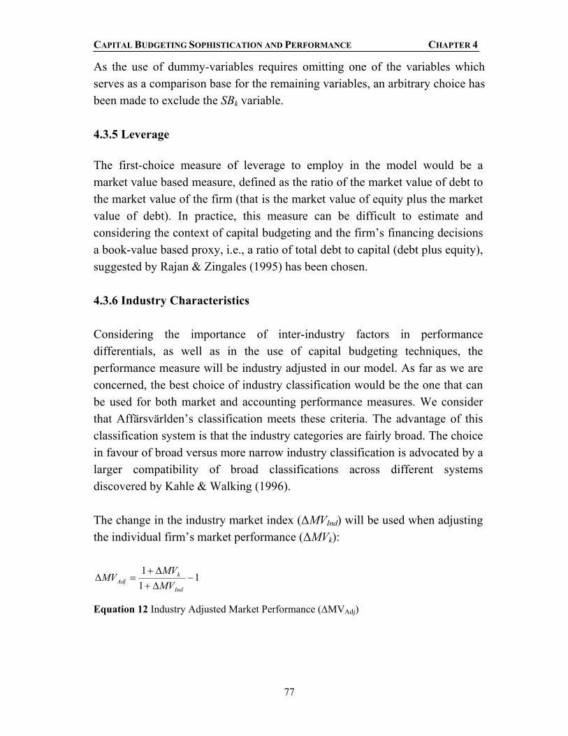
CAPITAL BUDGETING SOPHISTICATION AND PERFORMANCE CHAPTER 4
77
As the use of dummy-variables requires omitting one of the variables which serves as a comparison base for the remaining variables, an arbitrary choice has been made to exclude the SBk variable. 4.3.5 Leverage The first-choice measure of leverage to employ in the model would be a market value based measure, defined as the ratio of the market value of debt to the market value of the firm (that is the market value of equity plus the market value of debt). In practice, this measure can be difficult to estimate and considering the context of capital budgeting and the firm’s financing decisions a book-value based proxy, i.e., a ratio of total debt to capital (debt plus equity), suggested by Rajan & Zingales (1995) has been chosen. 4.3.6 Industry Characteristics Considering the importance of inter-industry factors in performance differentials, as well as in the use of capital budgeting techniques, the performance measure will be industry adjusted in our model. As far as we are concerned, the best choice of industry classification would be the one that can be used for both market and accounting performance measures. We consider that Affärsvärlden’s classification meets these criteria. The advantage of this classification system is that the industry categories are fairly broad. The choice in favour of broad versus more narrow industry classification is advocated by a larger compatibility of broad classifications across different systems discovered by Kahle & Walking (1996). The change in the industry market index (∆MVInd) will be used when adjusting the individual firm’s market performance (∆MVk):
111
−∆+∆+
=∆Ind
kAdj MV
MVMV
Equation 12 Industry Adjusted Market Performance (∆MVAdj)

CAPITAL BUDGETING SOPHISTICATION AND PERFORMANCE CHAPTER 4
78
Using the average value for ORRInd in the respective industry, the individual performance measures (ORRk) will be adjusted as follows:
111
−++
=Ind
kAdj ORR
ORRORR
Equation 13 Industry Adjusted Operating Rate of Return (ORRAdj)
Tobin’s q will be adjusted for each firm (qk) by subtracting the average Tobin’s q for the respective industry (qInd).
IndkAdj qqq −=
Equation 14 Industry Adjusted Tobin’s q (qAdj)
4.4 Comprehensive Description of General Model In order to clarify, the model developed in the previous sections is summarised below by a short presentation of the definitions and the resulting regression models. Three measures of performance are included in the model, of which the two first measures are accounting based and the last is market based. ORRAdjkt = Industry adjusted operating rate of return for firm k in year t. qAdjkt = Industry adjusted Tobin’s q for firm k in year t. ∆MVAdjkt = Industry adjusted yearly average change in stock market value for company k in year t. The following explanatory variables, formulated as below, are included in the model: SIZEkt = Size of firm k in year t, where size is defined as total assets. DRk = Degree of risk of firm k, where risk is defined as the standard deviation of the accounting performance measure used when accounting

CAPITAL BUDGETING SOPHISTICATION AND PERFORMANCE CHAPTER 4
79
performance measures are used, and defined as beta when market performance is applied. CIkt = Capital Intensity of firm k in year t, where capital intensity is defined as net fixed assets per employee. DEBTkt = Debt ratio of firm k in year t, where debt ratio is defined as the ratio of debt to capital (debt + equity). Dummy Variables for Diversification: DVk = Dominant Vertical strategy of a firm k (equal to 1 if this is the strategy, 0 otherwise) DCk = Dominant Constrained business strategy of a firm k (equal to 1 if this is the strategy, 0 otherwise) DLk = Dominant Linked strategy of a firm k (equal to 1 if this is the strategy, 0 otherwise) DUk = Dominant Unrelated strategy of a firm k (equal to 1 if this is the strategy, 0 otherwise) RCk = Related Constrained strategy of a firm k (equal to 1 if this is the strategy, 0 otherwise) RLk = Related Linked strategy of a firm k (equal to 1 if this is the strategy, 0 otherwise) UPk = Unrelated Passive strategy of a firm k (equal to 1 if this is the strategy, 0 otherwise) ACk = Acquisitive Conglomerates strategy of a firm k (equal to 1 if this is the strategy, 0 otherwise) The CBS variable will be defined either according to Definition I, II or III: CBS1k = Capital budgeting sophistication of firm k according to Def. I. CBS2k = Capital budgeting sophistication of firm k according to Def. II. CBS3k = Capital budgeting sophistication of firm k according to Def. III.

CAPITAL BUDGETING SOPHISTICATION AND PERFORMANCE CHAPTER 4
80
These definitions result in 9 regression models, defined as follows: Definition I:
tkkkkkkk
kktktkktkAdjkt
eAPUPRLRCDUDLDCDVDEBTCIDRSIZECBSORR
+++++++
+++++++=
8765432
15432110 δδδδδδδ
δββββββ
Equation 15 Regression Equation – CBS Definition I, ORRAdj
tkkkkkkk
kktktkktkAdjkt
eAPUPRLRCDUDLDC
DVDEBTCIDRSIZECBSq
+++++++
++++++++=
8765432
15432110
δδδδδδδ
δββββββ
Equation 16 Regression Equation – CBS Definition I, qAdj
tkkkkkkk
kktktkktkAdjkt
eAPUPRLRCDUDLDC
DVDEBTCIDRSIZECBSMV
+++++++
+++++++=∆
8765432
15432110
δδδδδδδ
δββββββ
Equation 17 Regression Equation – CBS Definition I, ∆MVAdj
Definition II:
tkkkkkkk
kktktkktkAdjkt
eAPUPRLRCDUDLDC
DVDEBTCIDRSIZECBSORR
+++++++
+++++++=
8765432
15432210
δδδδδδδ
δββββββ
Equation 18 Regression Equation – CBS Definition II, ORRAdj
tkkkkkkk
kktktkktkAdjkt
eAPUPRLRCDUDLDC
DVDEBTCIDRSIZECBSq
+++++++
+++++++=
8765432
15432210
δδδδδδδ
δββββββ
Equation 19 Regression Equation – CBS Definition II, qAdj
tkkkkkkk
kktktkktkAdjkt
eAPUPRLRCDUDLDC
DVDEBTCIDRSIZECBSMV
+++++++
+++++++=∆
8765432
15432210
δδδδδδδ
δββββββ
Equation 20 Regression Equation – CBS Definition II, ∆MVAdj
Definition III
tkkkkkkk
kktktkktkAdjkt
eAPUPRLRCDUDLDC
DVDEBTCIDRSIZECBSORR
+++++++
++++++++=
8765432
15432310
δδδδδδδ
δββββββ

CAPITAL BUDGETING SOPHISTICATION AND PERFORMANCE CHAPTER 4
81
Equation 21 Regression Equation – CBS Definition III, ORRAdj
tkkkkkkk
kktktkktkAdjkt
eAPUPRLRCDUDLDC
DVDEBTCIDRSIZECBSq
+++++++
+++++++=
8765432
15432310
δδδδδδδ
δββββββ
Equation 22 Regression Equation – CBS Definition III, qAdj
tkkkkkkk
kktktkktkAdjkt
eAPUPRLRCDUDLDC
DVDEBTCIDRSIZECBSMV
+++++++
+++++++=∆
8765432
15432310
δδδδδδδ
δββββββ
Equation 23 Regression Equation – CBS Definition III, ∆MVAdj
4.4.1 Quality of General Model – Validity and Practicality Emory and Cooper (1991) argue that a measurement tool can be considered of good quality if it is an accurate indicator of what one is interested in measuring. Additionally, it should be easy and efficient to use. Validity, reliability and practicality are three major considerations that can be used when evaluating a measurement tool. Therefore these three concepts have been applied to evaluate the quality of our model. Concerning the model constructed in this chapter, the validity and practicality of the model are the primary concerns. Since the reliability of the model is related to the empirical testing, it will be further discussed in Chapter 6. Validity can be defined as the extent to which differences found with a measuring tool reflect true differences among those being tested. In our case validity implies that differences in performance due to different degrees of capital budgeting sophistication, estimated by the model, reflect the true differences. The main difficulty in meeting the requirements of the validity test is however that the true differences usually are unknown. If they were known, one would not do the measuring in the first place. One aspect of validity is content validity, which is defined as the extent to which a measuring instrument provides adequate coverage of the topic under study (Emory & Cooper, 1991). Whether the definitions used include the relevant issues is hence a question of content validity. In order to achieve a high degree of content validity, the definitions used in the theoretical model are based on an extensive literature review on the subject.

CAPITAL BUDGETING SOPHISTICATION AND PERFORMANCE CHAPTER 4
82
Concerning the definition of the CBS variable in Definition I, two aspects need to be mentioned in relation to content validity. One aspect that might influence content validity is that the extent of usage cannot be considered, that is two respondent firms considering the same capital budgeting technique important will receive the same sophistication degree, regardless of the fact that the extent of usage may differ significantly. Since Definition II is, to a large extent, based on Definition I it is also assumed to be affected. The other aspect also concerns the definition of capital budgeting sophistication. As discussed before it was not feasible to consider the use of various capital budgeting techniques in a single metric of CBS Definition I. However, one could create a different model and define capital budgeting sophistication as, for example, the number of techniques used. As it is not possible to define which definition would better describe capital budgeting sophistication in a firm, the effect of the chosen approach on the validity cannot be estimated. This is important to remember when analysing the results. The choice of explanatory variables also affects the validity of the model. The omission of relevant variables, which is referred to as the omitted variable problem, may lead to a biased estimation of regression coefficients and may result in incorrect conclusions about the relationship between two main variables (Hill et al, 2001). This risk of omitted variable bias implies that one should take care to include all relevant variables. This can lead us to think that a good strategy is to include as many variables as possible in the regression model. However, doing so will not only complicate the model unnecessarily, it may inflate the variances of the regression estimates because of the presence of irrelevant variables (Ibid). Moreover, a large number of independent variables increase the risk of collinearity between variables. As a result the variance of the least square estimators may be large and, hence, may lead to wrong conclusions about the significance of the parameter estimates based on the t-test (Ibid). Therefore, the search for explanatory variables should be based on economic principles and logic reasoning, starting with the question, which variables are likely to influence the dependent variable, i.e., corporate performance. Practicality has also been considered in the process of the model construction. All variables used in the model have been defined taking into consideration the

CAPITAL BUDGETING SOPHISTICATION AND PERFORMANCE CHAPTER 4
83
feasibility of collecting all necessary data. For example, Definition I of the CBS variable considers that, due to simultaneous use of various capital budgeting techniques, it is not possible to consider all techniques in a single metric of sophistication. When defining Tobin’s q a simpler proxy has been suggested without an essential loss of informational content.


CAPITAL BUDGETING SOPHISTICATION AND PERFORMANCE CHAPTER 5
85
5. DATA
n order to test the constructed model empirically, data needed to be collected for the variables in consideration. For data collection purposes either primary
or secondary data can be used. Since secondary data can be especially useful when time and cost limitations are present (Emory & Cooper, 1991), we tried to use secondary data when possible. For the CBS variable both secondary data from a survey by Sandahl & Sjögren (2000) and primary data from an own survey was used. For the performance variable and other explanatory variables only secondary data was employed. Possible implications for the reliability and validity of the results, however, had to be considered in every case when secondary data is used. In the following sections, the data collection process, the reliability of data as well as data’s impact on the validity of the model are described.
5.1 Data for Defining Capital Budgeting Sophistication 5.1.1 Survey by Sandahl & Sjögren In order to estimate the CBS variable a survey performed by PhD Gert Sandahl and PhD Stefan Sjögren at the Department of Managerial Economics at Göteborg University (School of Economics and Commercial Law) was used. The study, which took place in the year 2000, concerns capital budgeting practices in Swedish companies. Sandahl and Sjögren offered us the opportunity to use the data set, which included information of great value for our thesis. The most important limitation with using this secondary data source was that the information only partly met our needs in terms of required data for testing the model. Neither the formulation of the questions nor the composition of the sample, which are crucial variables for the validity and reliability of a study, could be influenced (Emory & Cooper, 1991). These drawbacks were however considered to be of lesser importance than the advantages of time and cost reductions, which is why it was decided to use the data set although it demanded certain adjustments of our model.
The study performed by Sandahl & Sjögren (2002) aimed at presenting a general description of the art of capital budgeting in Swedish corporations. The
I

CAPITAL BUDGETING SOPHISTICATION AND PERFORMANCE CHAPTER 5
86
population considered was groups of companies with headquarters in Sweden. Additionally, they belonged to the Swedish top 500 companies26 or the companies listed on the O-list of the Stockholm Stock Exchange (SSE). An extensive questionnaire was sent to the headquarters of the selected 528 companies. The questionnaires were sent to the CFO or to the CEO of the respective company when no CFO was named in the database27. The incoming questionnaires confirmed that, in most cases, the person who the questionnaire was addressed to was the respondent (Ibid). Thereby one can assume that the risk of non-informed respondents, which is an often-mentioned weakness of mail surveys, is low (Kim, 1982). The first questionnaires were sent out on the 22 of June, 2000, and the third and last follow-up by mail was made in October 2000. Thereafter, selected companies were contacted by phone and encouraged to fill in the questionnaire. The procedure resulted in 128 responding firms, corresponding to a total response rate of 24.4%. Compared to the population, the respondent sample was biased towards large companies, and towards companies involved in manufacturing, construction, real estate, shipping and transport and public sector companies (Sandahl & Sjögren, 2002). Several tests were performed by Sandahl & Sjögren (2002) in order to investigate possible non-response bias. According to Rappaport (1979) and Kim (1982) firms with more sophisticated practices are assumed to be proud of this and thus generally more willing to respond to a questionnaire. The first test performed aimed at detecting non-response bias by comparing answers concerning the techniques used and the importance of quantitative factors from companies that returned the survey before the first reminder with those from companies responding after. The results showed that on the 5% level, the hypothesis “H0 = the later respondents display the same frequency distribution as the early respondents” could not be rejected. It was, however, not explicitly tested, whether the resulting sample was more sophisticated than the respondents not responding at all. Aggarwal (1980) suggests that this can be tested by performing a telephone or personal poll of a representative random sample of the non-respondents to see if their responses are different. The
26 As defined by Veckans Affärer 2000. (Sandahl & Sjögren, 2002) 27 Veckans Affärer, 2000 (Sandahl & Sjögren, 2002)
CAPITAL BUDGETING SOPHISTICATION AND PERFORMANCE CHAPTER 5
87
second test performed by Sandahl & Sjögren (2002) compared the respondents and non-respondents based on control variables. The results indicated that the sample was a good representation of the population considering industry and ownership. However, this was not true when accounting for size, since a bias towards larger companies existed (Ibid). The questions included in the survey focus on the financial evaluation and the selection procedures, and hence information concerning the entire investment process defined in Definition III could not be extracted from the survey. Possibly, a follow-up questionnaire concerning these issues could have been sent to the sample firms. The main problems associated with a follow-up questionnaire were that it would probably reduce the sample considerably and would also be very time-consuming. A lower number of respondents would negatively affect the reliability of the regression analysis, and hence it was decided not to use a follow-up questionnaire to complete the available data. This decision however means that we will not be able to accomplish an empirical test of Definition III. The amount of data obtained from the questionnaire is fairly extensive, but only a selected number of questions were used for the empirical testing. The questions were matched against the issues defined in the model as precisely as possible28. A major problem associated with using the data set was that few firms had answered all questions needed for us to test the model empirically. This fact has implications for our analysis since it will not be possible to consider all issues in a single metric in Definition II, in the way, which was accounted for in the general model. 5.1.2 Survey by Axelsson, Jakovicka & Kheddache In the majority of the earlier studies the respondent firms were asked to rank the relative importance of the components included in the CBS metric and based on these rankings scores were set (Kim, 1982; Pike, 1984; Farragher et al, 2001). This approach can however be seen as conflicting with the purpose of our study, which is to test a theoretical relationship empirically. We consider it
28 A presentation of the questions used and their interpretation is to be found in Appendix IV.

CAPITAL BUDGETING SOPHISTICATION AND PERFORMANCE CHAPTER 5
88
more appropriate to assign the scores theoretically rather than empirically. Therefore, we have chosen to adopt another approach that has been partly used by Pike (1986). This approach involves using scores set by academics. The objective in this case is to collect data concerning how academics, specialised in the area, understand the sophistication and importance of certain issues related to capital budgeting. Even though the available data set limited the possibilities of including Definition III of sophistication in the empirical tests, it was decided to include the third definition in the academic survey. The main reason for this choice is that the information gained from the academic survey could be used in order to improve the model29. According to Emory & Cooper (1991), the choice of sample technique should depend on the requirements of the project, its objectives, and funds available. Due to cost and time considerations, as well as the fact that generalisations to a population parameter were not of great interest for our study, nonprobability sampling was chosen in order to obtain scores for the CBS variable. Nonprobability sampling is non-random. Even though probability sampling, which is based on the concept of random selection, is technically superior to nonprobability sampling, the latter is more convenient if it, like in our case, meets the sampling objectives. The sample was made by judgement sampling, which occurs when the sample members are selected to conform to some predefined criterion (Ibid). With the assistance of our tutor PhD Gert Sandahl and PhD Stefan Sjögren, 14 Scandinavian academics with a specialisation within Managerial Economics, Economics or Management and Cost Accounting were chosen. Additionally, 9 American and British academics, which are among authors of earlier studies on the subject, were included in the sample. A questionnaire distributed by e-mail was chosen as the communication mode for the survey. It was considered appropriate, since the number of questions was limited and the response rates were assumed to be fairly high due to the characteristics of the sample (Emory & Cooper, 1991). The questionnaire presented the techniques and issues included in our definitions of capital budgeting sophistication, which the respondents were asked to evaluate. In order to avoid unnecessary and poorly formulated questions, we thoroughly 29 This will be further discussed in Section 5.2.

CAPITAL BUDGETING SOPHISTICATION AND PERFORMANCE CHAPTER 5
89
considered the function as well as the wording of each question when constructing the questionnaire. Furthermore, the questions were carefully discussed with our tutor PhD Gert Sandahl. Thereafter two pre-tests were undertaken including five academics at the Department of Managerial Economics at Göteborg University, School of Economics and Commercial Law. Since the test respondents belong to the same category as the sample group, their comments were very valuable. The objective of the questionnaire was to use the respondents’ answers as judgments concerning the sophistication and importance of a number of capital budgeting techniques and issues related to capital budgeting. The issues, which the academics were asked to assign scores to, are purely qualitative. According to Johnson & Wichern (1997) either a nominal or an ordinal scale can be used when dealing with qualitative variables. The values of the variables on a nominal scale are denoted by arbitrary labels or symbols. The ordinal scale is similar to the nominal scale but each name or symbol can be associated with the extent to which some underlying property is possessed. Since we are interested to know how sophisticated or important a number of issues are according to the respondents, an ordinal scale with sophistication and importance as underlying properties was chosen. Furthermore, a rating scale was used for evaluation, since it was considered more appropriate than a ranking scale. When using a ranking scale, the issues included in the comparison can be assumed to significantly influence the rankings. All kinds of scales do however have to be treated with care, since they are often misinterpreted. The rating scale used in our questionnaire largely depends upon the assumption that the respondents can and will make good assumptions. A common problem is that certain persons are “hard raters”, while others are “easy raters” (Emory & Cooper, 1991). Further, it is crucial to note that when using a subjective rating scale the answers are also subjective and the distance between the scores, for example, 3 and 4, and 4 and 5 cannot be estimated and can also diverge. One can hence not say that NPV is 0.5 more sophisticated than IRR, but only that NPV is more sophisticated than IRR. Additionally, the scale in terms of sophistication and importance as well as the distance between the numbers used in the scale, may be differently understood by the respondents. This may influence the comparability. Due to these facts it

CAPITAL BUDGETING SOPHISTICATION AND PERFORMANCE CHAPTER 5
90
would not be completely correct, from a statistical perspective, to compare the scores assigned and create an average score. However, an average score has been considered as the least bad alternative and has been used despite the existing deficiencies. An e-mail including a cover letter with a brief presentation of the study and an attached questionnaire was sent to the respondents on October 4, 2002 (see Appendix V). Additionally, the questionnaire was sent by post to one respondent, who preferred receiving it in this way. In order to increase the response rate a reminder was sent per e-mail on October 10, 2002, and thereafter selected respondents were contacted by phone. 10 complete answers were received (8 Scandinavian and 2 American respondents), which corresponded to a response rate of 40 %.
5.2 Academics’ View of Capital Budgeting Sophistication When interpreting the results presented below it is important to consider the deficiencies of using a qualitative ordinal scale. In the following paragraphs, the average scores will be presented. The complete distributions showing all individual scores for the most important issues are presented in Appendix VI. This additional information provides a possibility to evaluate the dispersion of the scores obtained as well as potential deficiencies related to using the average score.
Capital Budgeting Techniques
4
3,7
2,3
2,2
1,4
0 1 2 3 4 5
NPV
IRR
DPB
ARR
PB
Average Sophistication
Figure 7 Average score – Capital Budgeting Techniques

CAPITAL BUDGETING SOPHISTICATION AND PERFORMANCE CHAPTER 5
91
The sophistication scores assigned by academics were expected to result in high scores for NPV and IRR, and considerably lower scores for DPB, ARR and PB. As can be seen in Figure 7 above, the scores assigned did to a great extent correspond to these expectations. NPV and IRR received the highest average scores, 4 and 3.7 respectively. The deficiencies of IRR in comparison to NPV are hence visible. DPB is considered to be more sophisticated than ARR, but the answers of both these variables are relatively dispersed (see Appendix VI). As expected, PB received the lowest average sophistication score among the mentioned techniques.
Application of Sophisticated Capital Budgeting Techniques
3,2
3,7
3,7
3,9
4,3
0 1 2 3 4 5
Use of WACC
Tax consideration - cash flows
Tax consideration - discount rate
Consistnency - inflation
Consideration - firm / project risk
Average Importance/Sophistication
Figure 8 Average Score – Application of Capital Budgeting Techniques
Concerning the issues related to the application of sophisticated capital budgeting techniques, small differences in the average scores were expected. These expectations were met, as can be observed in Figure 8. The consideration of project and firm risk is assigned the highest score, while using the weighted average cost of capital (WACC) is assigned the lowest score. In an additional question, which was not included in the model, the academics were asked to assign a sophistication score to different ways of determining the discount rate. The most sophisticated method was the opportunity cost and thereafter WACC (see Appendix VI). This corresponds to literature on the subject that describes the opportunity cost of capital as the most correct cost of capital estimation and WACC as an approximation. It is important to note that the academics were requested to assign a score depending on the importance of the first four issues and based on sophistication for the last issue (issues related to WACC).

CAPITAL BUDGETING SOPHISTICATION AND PERFORMANCE CHAPTER 5
92
Issues related to WACC
4,1
3,7
3,9
0 1 2 3 4 5
CAPM
Market cost of debt
Market values debt & equity
Average Importance
Figure 9 Average Score – Issues Related to WACC When considering the issues related to the determination of WACC, small differences between the scores were expected. The average importance scores resulting from the academics’ subjective judgment also show small differences, and all scores are close to 4. As discussed before, we will not be able to incorporate Definition III of the CBS variable in the empirical tests since the information regarding the respondent firms’ practices is insufficient. This has the implication that also the scores concerning the capital budgeting process assigned by academics will not be used in the empirical tests. The results will however be presented and discussed, since they may indicate the quality of our theoretical model and may also be useful for future research. If an activity would receive a very low score, this might imply that it is not relevant enough to be included.

CAPITAL BUDGETING SOPHISTICATION AND PERFORMANCE CHAPTER 5
93
Capital Budgeting Process
4,1
3,4
3,3
3,3
3,8
4,0
3,3
4,1
3,0
3,8
3,8
0 1 2 3 4 5
Consideration of strategic aspects
Post-audits used to evaluate projects/improve future forecasts
Discounted cash flow techniques in post audits
Regular and pre-agreed upon procedures post-audits
Establishment of an implementation l assignment of project manager
Formal financial evaluation of proposals
The definition of alternative options for proposal
Formal process for screening investment proposals
Rewards to individuals that suggest good investments
Formal process for searching and id if i investment opportunities
Establishment of a long term capital
Average Score
Figure 10 Average Scores – Capital Budgeting Process
The respondents were asked whether they agreed that the presented activities were important when defining the degree of sophistication of a firm’s capital budgeting process. In this case 1 corresponded to “I strongly disagree” and 5 corresponded to “I strongly agree”. The respondents also had the opportunity to add activities, which they found important but that were not among the ones mentioned in the questionnaire. Only one respondent answered that he/she missed some important activities, which indicates that the activities included in our definition covered the main important ones. The answers obtained are presented in Appendix VI. The highest average sophistication scores (Figure 10) concern having a formal process for screening investment proposals,
CAPITAL BUDGETING SOPHISTICATION AND PERFORMANCE CHAPTER 5
94
consideration of strategic aspects and formal financial evaluation of investment proposals. Formal evaluation of investment proposals is also the activity that generally receives most attention in major literature. Rewards to individuals, who suggest good investment has been discussed by Mukherjee & Henderson (1987) as an interesting issue to consider, but got the lowest average score among the presented activities. All activities related to post-audits have also received noticeably low average scores. As a complement we asked the academics how important they considered the different stages of the process. This question was posed in order to see whether the results would be consistent with the more detailed activities mentioned above. The relation between the weights is in most cases consistent. It is interesting to note, however, that activities included in the post-audit stage received considerably lower scores than the post-audit stage (Appendix VI). Considering the whole questionnaire, we received some remarks from the respondents. Some respondents found the questions difficult to answer, since they considered the questions to be very context dependent. We are aware of this fact but in order to maintain the explanatory ability of the model, the number of issues considered in the matrices needed to be limited and therefore only general issues has been considered. Further, one respondent asked for the consideration of real options. Initially, we planned to incorporate this issue in the model, but since the use in Sweden is almost non-existent it was omitted (Sandahl & Sjögren, 2002).
5.3 Data for Defining the Performance Variable and the Explanatory Variables Internal secondary data was used in order to estimate the value of the dependent variable as well as the values of the independent explanatory variables. Internal secondary data is data that has already been produced by organisations or private individuals. The data is not collected to respond to the specific needs of the researcher, but constitutes a veritable data-source for those consulting it. Archives, reports and documents are examples of internal secondary data (Thiétart, 2001). Accounting data was collected mainly by using the database Amadeus. In the case of missing information, complementary data was collected by using the database Affärsdata and annual

CAPITAL BUDGETING SOPHISTICATION AND PERFORMANCE CHAPTER 5
95
reports available in the library and on the Internet. Market information was collected from the database EcoWin and the Affärsvärlden homepage. A 5-year time horizon (1997-2001) was applied, even though it would have been more appropriate to consider at least 15-years (Smith & Markland, 1981). This decision was made because available databases store data for the last five years at most, and collecting data manually for the years beyond this period would not be feasible considering the time restriction.
5.4 Reliability As already discussed, reliability is one of the factors determining a model’s quality (Emory and Cooper, 1991). Data and its quality are the main factors influencing the reliability of the model. The influence of these factors will be analysed below. A measure is described as reliable if it supplies consistent results. Reliability is concerned with the estimation of the degree to which a measurement is free of random or unstable error. This included a large number of firms in the sample that would, according to Emory and Cooper (1991), positively influence reliability. According to this argument, the small sample included in this study affects the reliability negatively. The 128 respondent firms in Sandahl’s and Sjögren’s sample constituted the initial sample in our empirical test of the theoretical model. Companies, for which performance data between 1997 and 2001 was incomplete due to mergers and acquisitions, were however excluded from this sample. Moreover, financial firms were excluded due to the peculiarity in terms of operations, structure of assets and liabilities that would hinder analysis and inter-company comparisons. Finally, those companies which indicated using such capital budgeting techniques that could not be attributed to any technique included in the theoretical model were also excluded from the sample. The final number of firms left in the sample was therefore reduced to 65, which is referred to as the Large Sample. The sample of 65 remaining companies was used to create a sub-sample of listed companies including 21 firms, which is referred to as the Small Sample. In Definition II the Large Sample varies from 56 to 62 firms and the Small Sample varies from 17 to 20 firms. This is due to the fact that not all firms have answered all questions relevant for Definition II.

CAPITAL BUDGETING SOPHISTICATION AND PERFORMANCE CHAPTER 5
96
Moreover, the short time period (5 years) used will negatively affect the reliability. Certain economic events may cause deviations in corporate performance from its long-run trend to persist for several years before reversing back to the trend (Smith & Markland, 1981). Such events can therefore cause distortion in measurement of the relationship between performance and capital budgeting sophistication. It is then important to consider that the characteristics of the time period might impose an additional problem. The period 1997-2002 was a turbulent period in the Swedish economy distinguished by both a boom and a recession. It is therefore, difficult to capture the true relationship between capital budgeting sophistication and performance. In the case of the questionnaire sent to academics, the number of respondents is low and might be considered negative for the reliability. However, since the objective of the questionnaire is not to generalise the results to the entire academic world, we do not assume this to have a negative influence on reliability. The reliability of the study was reinforced by the fact that accounting information provided by different databases was compared in order to verify the numbers. In the cases where the information differed in two databases a third data source was consulted (Amadeus, Affärsdata and corporate homepages).
5.5 Data Quality’s Effect on the Validity of the Model for Empirical Tests The validity of the model as discussed in Chapter 4 holds under the condition that all necessary data for the empirical testing can be collected. Data and its quality may however impose restrictions on the model, thereby affecting its validity. Unavailability of quantitative data, insufficient qualitative data and time constraints are the main reasons why the variables described in our model, in some cases, had to be redefined or excluded. Furthermore, certain adjustments were made to insure that the measures would suit the data. These adjustments will have a significant impact on the validity and will be discussed below.

CAPITAL BUDGETING SOPHISTICATION AND PERFORMANCE CHAPTER 5
97
Since qualitative data concerning firms’ capital budgeting processes was unavailable, Definition III of the CBS variable had to be excluded. This will affect the content validity negatively, since it has been argued that it is too narrow to define CBS only by considering the evaluation stage as in Definition I and Definition II (Kim, 1982; Pike, 1984; Pinches, 1982). Unfortunately, this cannot be altered and hence the lower degree of content validity has to be considered when analysing the results. Furthermore, it was not possible to use a single metric in Definition II, instead one issue at a time had to be considered. This was done by adjusting the sophistication degree from Definition I according to whether the firm considers taxes, inflation and so forth. Additionally, issue number two (consideration of taxes both in expected cash flows and the discount rate) had to be divided into two issues (2A “consideration of taxes in the expected cash flows” and 2B “consideration of taxes in the discount rate”). The reason for this is that the unavailability of qualitative information resulted in a excessively large number of missing values when considering the issues together in one variable. The weights for these issues (w2A and w2B) are calculated in the same way as weights for individual issues rather than sub-issues. The adjustments were made in the following manner.
)1()1()1(
)1(
)1(
)1(
)1(
441441441
331
221
221
111
ccjkkbbjkkaajkkk
jkkk
BBjkkk
AAjkkk
jkkk
wcCBSwcCBSwcCBSWACC
wcCBSPR
wcCBSTDR
wcCBSTCF
wcCBSINF
−×+−×+−×=
−×=
−×=
−×=
−×=
where, INFk = Capital budgeting technique adjusted for whether firm k takes into account inflation. TCFk = Capital budgeting technique adjusted for whether firm k takes into account taxes in the cash flow. TDRk = Capital budgeting technique adjusted for whether firm k considers taxes in the discount rate.

CAPITAL BUDGETING SOPHISTICATION AND PERFORMANCE CHAPTER 5
98
PRk = Capital budgeting technique adjusted for whether firm k accurately considers project risk. WACCk = Capital budgeting technique adjusted for whether firm k accounts for the weighted average cost of capital. The ORR had to be redefined since data concerning operating cash flows was not included in the information supplied by the database Affärsdata. It would be too time consuming to gather complementary information for all companies and years where this information was missing. The most appropriate alternative, operating profit (loss)30, was instead used as the numerator in operating rate of return ratio. This redefinition might affect the validity of the model negatively since the operating profit is more subject to distortions, due to accruals, than the operating cash flow. The denominator of the operating rate of return was also redefined. Theoretically, it is most appropriate to use the average value for total assets for the respective year in the denominator. However, since the period studied only covers five years and using the yearly average asset value would reduce the number of observations, it was decided to use total assets31 per year in the denominator instead of the average. The advantage of having five instead of four observations was considered greater than the disadvantage of using total assets in the denominator. Tobin’s q was excluded since information concerning the number of outstanding shares could not be obtained from Amadeus and Affärsvärlden. Sources for this information are annual reports. However, due to time constraints this option was not considered. The omission of Tobin’s q will limit our ability to compare the results concerning the different performance measures. When the empirical relationship between size and performance was analysed in our data set, it was discovered that the relationship was not linear and could be better characterised as an increasing function of size in relation to performance, but at a decreasing rate. This is consistent with the theoretic arguments that size can contribute to improved performance. As the size increases, the benefits of increased size measured by performance might not increase at the same rate, as 30 Operating Profit (Loss) is more closely defined as the gross profit minus other operating expenses (Amadeus, 2002). 31 Total assets can be broken down into fixed assets (intangible fixed assets, tangible fixed assets and other fixed assets including financial fixed assets) and current assets (stocks, debtors and other current assets) (Amadeus, 2002).

CAPITAL BUDGETING SOPHISTICATION AND PERFORMANCE CHAPTER 5
99
they will be outweigh by disadvantages of size. Therefore, a logarithmic transformation, where size is defined as the natural logarithm of total assets, suggested in a study by Beaver et al (1970) has been tested. The tests resulted in a higher significance (t-test) of the size variable as well as a higher R2 of the regression model. Moreover, the distribution of the size variable was found to conform more nearly to the properties of symmetry and normality tested using kurtosis32 and skewness33. The data availability problem can be considered to have a negative effect of the quality of the risk measures in the model. Due to unavailability of data and time constraints, the standard deviation of ORR could only be estimated over a period of 5 years, which reduces the statistical quality of the standard deviation measure itself as well as its ability to measure the risk of a firm. Additionally, the accounting based risk measure is affected by its orientation towards “future”, i.e., in a regression model for 1997 the risk measure calculated over the period 1997-2001 is used. Similar reservations about the quality of beta as a risk measure can be made, where the same beta values are used for the yearly regression models. This can only be done under the assumption that beta values are stationary, i.e., they do not vary from period to period. However, this assumption has not been tested and as beta values have been collected during October 2002, recent events on the stock market, especially taking into consideration the sharp decline in stock prices during the latter part of the time period, could have influenced the beta values. Moreover, additional reservation concerning the use of beta as a risk measure has to be made in view of the composition of the sample tested. The sample is biased towards large firms, often holding companies with diverse divisions. It raises the issue whether beta is able to reflect different characteristics of risk attributable to diverse divisions of such companies. The measure of leverage suggested as the best alternative in the context of capital budgeting, i.e., the ratio of total debt to capital (debt plus equity), needed to be redefined in view of the unavailability of data. The second-best 32 Kurtosis is a measure of ”peakedness” of the distribution and for normal distribution the kurtosis value is 3 (Hill et al, 2001). 33 Skewness refers to how symmetric observations are distributed around their mean and perfectly symmetric distribution has a skewness of zero (Hill et al, 2001).

CAPITAL BUDGETING SOPHISTICATION AND PERFORMANCE CHAPTER 5
100
measure would be the ratio of debt to total assets adjusted by “accounts payable” and “other liabilities”. However, the balance sheet item “other liabilities” was not available for the firms in the sample, for which data was obtained from the Affärsdata database. Instead, the ratio of debt34 to total assets adjusted only by “accounts payable”, was employed. Using this measure can to some extent negatively affect the validity of the model. First of all, it includes such balance sheet items as pension liabilities and “other liabilities” that do not constitute debt from a theoretic perspective and, hence, might overestimate leverage. Moreover, as accounts payable enter the denominator of the leverage measure, a large size of accounts payable relative to equity, especially in years followed by consecutive losses, inflated the measure of leverage for some companies in our sample. Considering the fact that Rumelt’s measure of diversification requires a detailed analysis of a firm’s revenues in order to determine the firm’s diversification strategy, the diversification variable was omitted in the regression model. The potential effect of the omission to a large extent depends on how strong the relationship between diversification and performance is in our sample. In case of a strong relationship, the omission of the diversification variable might lead to an omitted-variable bias, resulting in biased regression estimators. On the other hand, if the relationship is weak or if diversification has no effect on performance, its omission would not have any effect on the results. In order to be able to compare the results obtained using market and accounting based measures, one should choose an industry classification system, which can be used for both market and accounting performance. The Affärsvärlden classification system consisting of 9 industry groups and 30 sub-groups was suggested in Chapter 4. However, it only provides information for listed companies, hence, in our sample it could only be used for the sub-sample of listed firms. For firms that are not listed on the SSE, we would need to assign industry categories manually. This would require a deep knowledge of firms’ activities and procedures, information on which Affärsvärlden’s classification 34 Debt consists of non-current liabilities (that is, long term debt and other non current liabilities including provision) and current liabilities (loans, creditors and other current liabilities).

CAPITAL BUDGETING SOPHISTICATION AND PERFORMANCE CHAPTER 5
101
is based. Therefore, a decision was made to use the Swedish National Industry classification system, SNI, for the sample with accounting-based performance measures. The SNI classification system is much broader than that of Affärsvärlden, hence, two-digit categories have been used. For some companies, however, more narrow industry codes have been assigned. It concerns mostly the industry category named “other activities”, which combines heterogeneous types of activities. An additional reservation has to be made regarding the industry adjustments based on the SNI classification. The data for these adjustments was obtained from the Amadeus database, which is biased towards large companies35. Even though it is claimed by Kahle &Walking (1996), that different classification systems are compatible for 64% of the companies in USA on a two-digit code basis, it is difficult to estimate differences in various classification systems in Sweden as well as their effect on the validity of the model. To conclude, the available data will to a large extent affect the empirical test of the model constructed. Based on the prevailing conditions the most feasible alternatives have however been used when conducting the empirical tests in order to be able to fulfill the purpose of the thesis to the largest possible extent.
5.6 Summary – Model for Empirical Tests As discussed above, the model had to be reformulated due to insufficient data quality and difficulties finding certain data. The following sections summarise the model as it is formulated for the empirical tests. Two measures of performance will be used: ORRAdjkt = Industry adjusted operating rate of return for firm k in year t. ∆MVAdjkt = Industry adjusted yearly average change in stock market value for company k in year t.
35 To be included in the Amadeus database a company should satisfy at least one of the following size criteria: (1) operating revenue equal to at least 10 million €, (2) total assets equal to at least 20 million €, (3) number of employees equal to at least 100 (Amadeus, 2002).

CAPITAL BUDGETING SOPHISTICATION AND PERFORMANCE CHAPTER 5
102
The following explanatory variables, formulated as below, will be used: ln SIZEkt = The natural logarithm of firm k’s size (defined as total assets) in year t, where size is defined as total assets. DRk = Degree of risk of firm k, where risk is defined as the standard deviation of the accounting performance measure used when accounting performance measures are used, and defined as beta when market performance is applied. CIkt = Capital Intensity of firm k in year t, where capital intensity is defined as net fixed assets per employee. DEBTkt = Debt ratio of firm k in year t, where debt ratio is defined as the ratio of debt to total assets adjusted by accounts payable. Definition I of the CBS variable is the following: CBS1k = Capital budgeting sophistication of firm k according to Definition I. Since a single metric could not be applied, CBS Definition II consists of 5 sub definitions, which are tested one at a time: TCFk = Capital budgeting sophistication adjusted for whether firm k takes into account taxes in the cash flow. TDRk = Capital budgeting sophistication adjusted for whether firm k considers taxes in the discount rate. INFk = Capital budgeting sophistication adjusted for whether firm k takes into account inflation. PRk = Capital budgeting sophistication adjusted for whether firm k accurately considers project risk. WACCk = Capital budgeting sophistication adjusted for whether firm k accounts for the weighted average cost of capital. In order to test the two models (Model I and Model II corresponding to CBS Definition I and CBS Definition II) 18 regressions equations will be estimated and are defined as follows:

CAPITAL BUDGETING SOPHISTICATION AND PERFORMANCE CHAPTER 5
103
Model I For the large sample36, Definition I:
tktktkktkAdjkt eDEBTCIDRSIZECBSORR ++++++= 5432110 ln ββββββ
Equation 24 Model I for Empirical Test - Large Sample
For the small sample37, Definition I:
tktktkktkAdjkt eDEBTCIDRSIZECBSORR ++++++= 5432110 ln ββββββ
tktktkktkAdjkt eDEBTCIDRSIZECBSMV ++++++=∆ 5432110 ln ββββββ
Equation 25 Model I for Empirical Test - Small Sample
Model II For the large sample38, Definition II:
tktktkktkAdjkt eDEBTCIDRSIZETCFORR ++++++= 543210 ln ββββββ
tktktkktkAdjkt eDEBTCIDRSIZETDRORR ++++++= 543210 ln ββββββ
tktktkktkAdjkt eDEBTCIDRSIZEINFORR ++++++= 543210 ln ββββββ
tktktkktkAdjkt eDEBTCIDRSIZEPRORR ++++++= 543210 ln ββββββ
tktktkktkAdjkt eDEBTCIDRSIZEWACCORR ++++++= 543210 ln ββββββ
Equation 26 Model II for Empirical Test - Large Sample
For the small sample39, Definition II:
tktktkktkAdjkt eDEBTCIDRSIZETCFORR ++++++= 543210 ln ββββββ
tktktkktkAdjkt eDEBTCIDRSIZETDRORR ++++++= 543210 ln ββββββ
tktktkktkAdjkt eDEBTCIDRSIZEINFORR ++++++= 543210 ln ββββββ
tktktkktkAdjkt eDEBTCIDRSIZEPRORR ++++++= 543210 ln ββββββ
36 Sample including 65 quoted and non-quoted firms. 37 Sample including 21 quoted firms. 38 Since all firms did not answer all questions, the sample size ranges between 56 and 62 firms in the test of Definition II. 39 Since all firms did not answer all questions, the sample size ranges between 17 and 20 firms in the test of Definition II.

CAPITAL BUDGETING SOPHISTICATION AND PERFORMANCE CHAPTER 5
104
tktktkktkAdjkt eDEBTCIDRSIZEWACCORR ++++++= 543210 ln ββββββ
tktktkktkAdjkt eDEBTCIDRSIZETCFMV ++++++=∆ 543210 ln ββββββ
tktktkktkAdjkt eDEBTCIDRSIZETDRMV ++++++=∆ 543210 ln ββββββ
tktktkktkAdjkt eDEBTCIDRSIZEINFMV ++++++=∆ 543210 ln ββββββ
tktktkktkAdjkt eDEBTCIDRSIZEPRMV ++++++=∆ 543210 ln ββββββ
tktktkktkAdjkt eDEBTCIDRSIZEWACCMV ++++++=∆ 543210 ln ββββββ
Equation 27 Model II for Empirical Test - Small Sample

CAPITAL BUDGETING SOPHISTICATION AND PERFORMANCE CHAPTER 6
105
6. EMPIRICAL TESTS ON THE SWEDISH MARKET n this chapter the empirical results are presented and analysed. The first part accounts for a presentation of the results. These results will then be analysed
in the second part.
6.1 Presentation of Empirical Results 6.1.1 Model I Model I including CBS Definition I was the first model to be tested. Capital budgeting sophistication is in this case evaluated on the basis of whether a firm uses NPV, IRR, DPB, ARR or PB. Two definitions of performance were used, i.e., the industry adjusted operating rate of return, ORRAdj, and the industry adjusted yearly average stock market change, ∆MVAdj. Large Sample In the regression equation for the large sample the accounting measure of performance, ORRAdj, is used. The results for the time period 1997-2001 are presented in Table 1.
Table 1 Estimated Regression Coefficients - Large Sample, Model I
* Significance at a 0.01 level ** Significance at a 0.05 level N/F = Model not significant (F-test)
I
1997 1998 1999 2000 2001 Average
1997-2001CBS Def I -0.0217** -0.0183* -0.0064 -0.0010 -0.0029 -0.0105 Ln Size 0.0072 0.0099* 5.5E-10** 0.0065 0.0073 0.0091* Risk SD -0.2416 -0.7237* -0.7432** -0.1197 -2.2125** -0.7730**Capital Intensity 0.0001 -0.0003 -0.0003 -0.0006 -0.0011 -0.0006 Leverage -0.0314 -0.0555 -0.0187 -0.0533 -0.0513 -0.0407 F-test (p-value) 0.0690 0.0086 0.0197 0.4869 0.0000 0.0010 Model Significance N/F 0.01 0.05 N/F 0.01 0.01 (Sample size:65)
CAPITAL BUDGETING SOPHISTICATION AND PERFORMANCE CHAPTER 6
106
The resulting regression coefficients for the CBS variable are negative for all years. This implies that the more sophisticated capital budgeting techniques a firm uses the worse it will perform in terms of ORRAdj, under the assumption that all other explanatory variables are kept constant. For year 1997 the regression coefficient is significant (t-test) at a 0.01 level and for 1998 it is significant at a 0.05 level. For all other years and the average period the regression coefficients are also negative but insignificant. Furthermore, the model itself appears insignificant in 2000 as the null hypothesis cannot be rejected when performing the F-test. The same set of regressions were also run using dummy variables for the five different capital budgeting techniques.
tktkt
kktkkkkAdjkt
eDEBTCI
DRSIZEDPBARRIRRNPVORR
++
+++++++=
43
2143210
ββ
ββδδδδβ
Equation 28 Regression Equation – Large Sample, Model I, Dummies
The reason for using dummy variables is that the rating scale applied, when constructing the CBS variable, can be statistically questioned, while the use dummies is statistically correct. We intended to confirm whether the results obtained would differ between using the CBS variable, based on the rating scale, and the dummy variables. Large differences could imply that the rating scale may cause statistical problems and produce biased results. The regression coefficients obtained when using the dummy variables are presented in Table 2.

CAPITAL BUDGETING SOPHISTICATION AND PERFORMANCE CHAPTER 6
107
Table 2 Estimated Regression Coefficients - Large Sample, Model I, Dummies * Significance at a 0.01 level ** Significance at a 0.05 level N/F = Model not significant (F-test) Considering the characteristics of dummy variables when the intercept is included, the results should be interpreted in relation to the omitted variable, PB. Hence, in 1997 firms using PB perform better than firms using any of the other capital budgeting techniques under the assumption that all other explanatory variables are kept constant. Since the coefficient is smaller for NPV and IRR than for DPB and ARR this implies that the more sophisticated techniques a firm uses the worse it performs, in relation to firms using PB. Approximately the same result is obtained for 1998 and 1999. In 2000 the situation is the reverse, i.e., firms using either NPV, IRR, DPB or ARR perform better that firms using PB. In 2001, the results signify that firms using PB perform better than firms using NPV, IRR but worse than firms using ARR and DPB. Most of the results are insignificant and hence no strong conclusions can be drawn. It is important to note that the whole regression model is insignificant in 1999 and 2000 (F-test). The regression coefficients obtained when using the CBS variable and the regression coefficients obtained using dummy variables are to a large extent similar. Therefore, we can conclude that the use of the rating scale for the CBS variable does not necessarily result in wrongly estimated regression coefficients.
1997 1998 1999 2000 2001 Average
1997-2001NPV -0.0659** -0.0401 -0.0238 0.0013 -0.0030 -0.0248 IRR -0.0800* -0.0723 -0.0243 0.0142 -0.0087 -0.0329 DPB -0.0574* -0.0216 -0.0155 0.0094 0.0006 0.0168 ARR 0.0199 0.0244 0.0123 0.0402 0.0257 0.0157 Ln Size 0.0112** 0.0118* 0.0114* 0.0068 0.0081 0.0097* Risk SD -0.0998 -0.5933 -0.5434* -0.0908 -2.1674** -0.7152**Capital Intensity -0.0001 -0.0004 -0.0005 -0.0005 -0.0012 -0.0007 Leverage -0.0544 -0.0750 -0.0368 -0.0673 -0.0611 -0.0527 F-test (p-value) 0.0180 0.0220 0.1047 0.6169 0.0000 0.0057 Model Significance 0.05 0.05 N/F N/F 0.01 0.01 (Sample Size: 65)

CAPITAL BUDGETING SOPHISTICATION AND PERFORMANCE CHAPTER 6
108
The pairwise relationship between CBS and performance, defined as ORRAdj, was tested through correlation analyses. The correlation tables can be found in Appendix VIII. The correlation between the variables is negative for all years except for 2000 and 2001. These results correspond to the results obtained from the regression models for the period 1997-1999. The estimated regression coefficients for the explanatory variables are also presented in Table 1 and 2. Size (measured in 1000 SEK) is found to exhibit a consistent positive relationship with performance in both the regression equations with the CBS variable and the regression equations with dummies. The regression coefficients appear to be significant for 1997 (only when dummies are used), 1998, 1999 and in the average period. The analysis of the pairwise correlation between size and performance also supports the existence of a positive relationship (see Appendix VIII). The estimated regression coefficients for capital intensity (measured in 1000000 SEK per employee) are mostly negative and exclusively insignificant in both the regression equations with the CBS variable and the regression equations with dummies. The correlation analysis shows that the relationship between capital intensity and performance is negative, although the correlation is very small. The estimated regression coefficients for risk are all negative and significant for 1998 (only when using the CBS variable), 1999, 2001 and for the average period in both the regression equations with the CBS variable and the regression equations with dummies. The correlation analysis also indicates a consistently negative relationship between risk and performance. Both the regression equations with the CBS variable and the regression equations with dummies produce insignificant negative coefficients for leverage and performance. The correlation matrices also show a consistently negative correlation between the two variables. Only in year 2001 is the correlation positive but very small. The regression assumptions are necessary conditions to ensure that the regression analysis is performed correctly and that the regression estimators are BLUE40. The assumptions that are feasible to test have been tested for the large sample when the CBS variable is used. These tests are to be found in Appendix IX. For 1997 all assumptions are fulfilled. Assumption 3 of homoskedasticity is
40 Best Linear Unbiased Estimators (BLUE) (Hill et al, 2001).

CAPITAL BUDGETING SOPHISTICATION AND PERFORMANCE CHAPTER 6
109
not fulfilled in the remaining years. Assumption 6 is not fulfilled in 1999-2001 and in the average period. Small Sample In the regression equation for the small sample both the market performance measure ∆MVAdj and the accounting measure of performance ORRAdj are used. ORRAdj is employed also in this case since it allows for the possibility to compare potential differences in outcomes when using the two performance measures. The results are presented in Table 3. Before the significance of the individual regression coefficients is discussed it has to be pointed out that the whole regression model is insignificant when using ORRAdj for 1997, 1999 and the average period (F-test). When ∆MVAdj is used the whole regression model is insignificant for all years except for the average period. This result may be caused by the extremely small sample size. Negative and insignificant results for the individual coefficients are obtained for the period 1997-1999 both when using ORRAdj and ∆MVAdj. For the time period 2000-2001 as well as for the average period the regression equation using ORRAdj still produces negative results, however, using ∆MVAdj positive regression coefficients are obtained. Among these coefficients the only significant result is obtained in year 2000 using ORRAdj. Even though approximately all results are insignificant, they are almost exclusively negative, signifying that companies using sophisticated capital budgeting techniques perform worse than companies that do not. Dummy variables were used also in this case in order to draw conclusions about whether the rating scale could be used.
tktkt
kktkkkkAdjkt
eDEBTCIDRSIZEDPBARRIRRNPVORR
+++
+++++++=
43
2143210 ββ
ββδδδδβ
Equation 29 Regression Equation - Small Sample, Model I, Dummies, ORRAdj
tktkt
kktkkkkAdjkt
eDEBTCIDRSIZEDPBARRIRRNPVMV
+++
+++++++=∆
43
2143210 ββ
ββδδδδβ
Equation 30 Regression Equation - Small Sample, Model I, Dummies, ∆MVAdj

CAPITAL BUDGETING SOPHISTICATION AND PERFORMANCE CHAPTER 6
110
The results obtained are presented in Table 4. In this case the whole model is only significant in 1999 when using both ORRAdj and ∆MVAdj and in 2001 when using ORRAdj (F-test). The regression coefficients obtained when using dummy variables do to a large extent coincide with those obtained when using the CBS variable. For the time period 1997-1999, companies using any of the techniques presented in Table 4 seem to perform worse than a company using PB. These outcomes are obtained both when using ∆MVAdj and ORRAdj. The results are however insignificant. Using ∆MVAdj the results becomes the reverse in 2000 and 2001 while when using ORRAdj the results still point at the fact that PB is superior to all the other capital budgeting techniques. The results obtained when running the regression for the average period signify that firms using NPV perform worse than firms using PB. This is true both when ∆MVAdj and ORRAdj is used as the dependent variable. The results are, also in this case, insignificant. The correlation between CBS and ∆MVAdj is negative as well as the correlation between CBS and ORRAdj. This result is consistent with the estimated regression coefficients. It is interesting to note that the correlation between the CBS variable and ORRAdj is more negative than the correlation between the CBS variable and ∆MVAdj The correlation table for the time period 1997-2001 can be found in Appendix VIII. The regression coefficients for the explanatory variables in the small sample will not be presented in much detail due to a low significance of the regression models (F-test). The regression coefficients for size using ORRAdj in both the regression equations with the CBS variable and the regression equations with dummies confirm the positive relationship established for the whole sample, while the regression coefficients for size using ∆MVAdj are mixed. The coefficients for capital intensity in both the regression equations with the CBS variable and the regression equations with dummies (using both ORRAdj and ∆MVAdj) are more mixed than in the whole sample but are mostly insignificant. When employing ORRAdj the relationship between risk and performance is negative. Beta is employed as a measure of risk in the regression models using ∆MVAdj as a performance measure. For the regression model with the CBS

CAPITAL BUDGETING SOPHISTICATION AND PERFORMANCE CHAPTER 6
111
variable and for the regression model with dummies the relationship between beta and ∆MVAdj is negative in half of the cases and positive in the rest. The coefficients are to a large extent insignificant. The estimated regression coefficients for leverage are mixed and are also mostly insignificant.

112
Tab
le 3
Est
imat
ed R
egre
ssio
n C
oeff
icie
nts -
Sm
all S
ampl
e, M
odel
I
* Si
gnifi
canc
e at
a 0
.01
leve
l **
Sig
nific
ance
at a
0.0
5 le
vel
N/F
= M
odel
not
sign
ifica
nt (F
-test
)
19
97
1998
19
99
2000
20
01
Ave
rage
19
97-2
001
O
RR
Adj
∆M
V
OR
RA
dj∆M
V
OR
RA
dj∆M
V
OR
RA
dj
∆MV
O
RR
Adj
∆MV
O
RR
Adj
∆MV
C
BS
Def
I -0
.032
4 -0
.036
8-0
.057
2-0
.022
9-0
.088
1-0
.016
2 0.
0293
-0
.034
7*0.
1139
-0
.027
20.
0141
-0
.021
0Ln
Siz
e 0.
0039
-0
.041
60.
0128
0.00
964.
7E-1
0-7
.1E-
100.
0187
* 0.
0403
0.
0143
0.
0216
0.
0071
-0
.023
1R
isk
SD/B
eta
-0.0
468
-0.1
418
-0.0
202
-0.1
031
-0.0
475
0.05
35
-0.0
350
0.11
86
-0.0
340
0.03
94
-0.0
487
-0.0
720
Cap
ital I
nten
sity
0.
0249
-0
.018
4-0
.036
0-0
.117
3-0
.032
60.
2688
0.
0011
-0
.018
9 -0
.010
0-0
.043
8-5
.762
5*-2
3.47
69Le
vera
ge
0.03
26
0.24
54-0
.020
7-0
.364
40.
0198
0.
1532
0.
0338
-0
.083
2 -0
.003
60.
0108
0.
1278
0.
5881
F-
test
(p-v
alue
) 0.
5519
0.
6525
0.08
110.
4198
0.10
16
0.22
66
0.07
06
0.59
16
0.03
49
0.62
63
0.13
19
0.00
18
Mod
el S
igni
fican
ce
N/F
N
/F
N/F
N
/F
N/F
N
/F
N/F
N
/F
0.05
N
/F
N/F
0.
01
(Sam
ple
size
: 21)

113
Tab
le 4
Est
imat
ed R
egre
ssio
n C
oeff
icie
nts -
Sm
all S
ampl
e, M
odel
I, D
umm
ies
* Si
gnifi
canc
e at
a 0
.01
leve
l **
Sig
nific
ance
at a
0.0
5 le
vel
N/F
= M
odel
not
sign
ifica
nt (F
-test
)
19
97
1998
19
99
2000
20
01
Ave
rage
19
97-2
001
O
RR
Adj
∆M
V
OR
RA
dj∆M
V
OR
RA
dj
∆MV
O
RR
Adj
∆M
V
OR
RA
dj
∆MV
O
RR
Adj
∆MV
N
PV
-0.1
060
-0.1
571
-0.0
225
-0.1
648
-0.0
478
-0.2
139
-0.0
436
0.06
53
-0.0
175
0.33
02-0
.035
7-0
.022
8IR
R
-0.1
319*
-0.
1094
-0.1
053
-0.1
271
-0.0
403
-0.1
129
-0.0
075
0.12
41
-0.0
493
0.22
65-0
.055
20.
0161
D
PB
-0.1
199
-0.3
587
-0.0
496
0.04
24-0
.062
80.
1796
-0
.090
9 0.
3249
-0
.000
6 0.
4781
-0.0
718
0.14
83
AR
R
-0.0
852
-0.3
813
-0.0
470
-0.0
630
-0.0
473
-0.4
919*
-0.0
278
-0.1
347
0.01
22
0.46
65-0
.037
5-0
.120
7Ln
Siz
e 0.
0197
-0
.046
00.
0136
0.01
220.
0227
**-0
.054
70.
0080
0.
0409
0.
0029
0.
0567
0.01
46
0.00
10
Ris
k SD
/Bet
a -0
.139
0 -0
.115
80.
1831
-0.1
162
-0.9
012*
0.00
88
0.57
12*
0.08
89
-2.0
680*
-0.0
028
-0.4
913
-0.0
277
Cap
ital I
nten
sity
0.
0159
-0
.009
2-0
.063
1-0
.091
3-0
.032
60.
2856
0.
0038
-0
.012
8-0
.021
6*-0
.036
9-0
.015
70.
0088
Le
vera
ge
0.01
17
0.65
50-0
.013
7-0
.330
1-0
.068
10.
5133
0.
0284
0.
0290
-0
.102
0 -0
.273
5-0
.034
30.
0903
F-
test
(p-v
alue
) 0.
2775
0.
8611
0.11
770.
7790
0.04
01
0.02
51
0.66
01
0.62
84
0.00
67
0.66
680.
1488
0.
6648
M
odel
Sig
nific
ance
N
/F
N/F
N
/F
N/F
0.
05
0.05
N
/F
N/F
0.
01
N/F
N
/F
N/F
(S
ampl
e si
ze: 2
1)

CAPITAL BUDGETING SOPHISTICATION AND PERFORMANCE CHAPTER 6
114
6.1.2 Model II Model II including CBS Definition II does not only take into account what technique is used but also how it is used. The original idea was to include all capital budgeting issues in one single metric. This was however not possible due to insufficient data. The alternative solution was to test each of the issues separately. Large Sample In the regression equation for the large sample the relationship between the different adjusted CBS variables and ORRAdj was estimated. The results obtained are presented in Table 5.
Table 5 Estimated Regression Coefficients - Large Sample, Model II * Significance at a 0.01 level ** Significance at a 0.05 level N/F = Model not significant (F-test) Before the significance of the individual regression coefficients is discussed it is important to note that, according to the F-test, the regression models incorporating TCF and INF are insignificant only in year 2000. For PR and
Sample
Size 1997 1998 1999 2000 2001
Average 1997-2001
TCF 59 -0.0415** -0.0234 -0.0188 0.0007 0.0016 -0.0151 F-test (p-value) 0.0009 0.0051 0.0004 0.2980 0.0000 0.0002 Model Significance 0.0100 0.0100 0.0100 N/F 0.0100 0.0100 TDR 60 -0.0316** -0.0249* -0.0157 0.0042 -0.0130 -0.0157 F-test (p-value) 0.0253 0.0744 0.0597 0.3925 0.0000 0.0152 Model Significance 0.0500 N/F N/F N/F 0.0100 0.0500 INF 56 -0.0345** -0.0263* -0.0201* -0.0068 -0.0067 -0.0191* F-test (p-value) 0.0009 0.0030 0.0031 0.3645 0.0000 0.0003 Model Significance 0.0100 0.0100 0.0100 N/F 0.0100 0.0100 PR 60 -0.0330** -0.0188 -0.0088 -0.0028 -0.0010 -0.0115 F-test (p-value) 0.0258 0.0492 0.0649 0.4326 0.0000 0.0041 Model Significance 0.0500 0.0500 N/F N/F 0.0100 0.0100 WACC 62 -0.0336** -0.0240* -0.0133 -0.0039 -0.0128 -0.0154 F-test (p-value) 0.0038 0.0263 0.0737 0.4531 0.0000 0.0027 Model Significance 0.01 0.05 N/F N/F 0.01 0.01

CAPITAL BUDGETING SOPHISTICATION AND PERFORMANCE CHAPTER 6
115
WACC, the regression models are insignificant in 1999 and 2000, and for TDR the regression models in the period 1998-2000 are insignificant. Considering the individual regression coefficients, they are almost exclusively negative for all issues for the whole period. The negative outcomes for year 1997 are significant at a 0.01 level (t-test). The regressions run for the period 1998-1999 also gave significant results for some of the adjusted CBS variables (TDR, INF and WACC). All estimated significant coefficients are negative. Some positive relationships have also been captured. The relationship between ORRAdj and the CBS variables adjusted for tax considerations is positive and insignificant for year 2000 (TCF and TDR) and 2001 (TCF). When testing the regression for the average period only negative results are obtained. The relationship between INF and ORRAdj was the only significant outcome in this case. Small Sample Information from the smaller subset, consisting of listed companies, was used in order to test the relationship between the adjusted CBS variables and ∆MVAdj. In order to be able to compare possible differences in outcomes arising from the fact that two types of performance measures are used, an estimation of the relationship between the adjusted CBS variables and ORRAdj is also accomplished for this sample. The results obtained are presented in Table 6. Due to the small sample size, a fairly large number of the regression models are insignificant. For TCF the regression model is only significant in 2001 when using ORRAdj and in 1999 when using ∆MVAdj. For TDR and INF the regression models are insignificant for the periods 1997-1998 and 2000-2001, when ∆MVAdj is applied. For INF the regression model, when using ORRAdj as the dependent variable, is insignificant in 2000. Concerning PR, the regression models are only significant for 1999 when applying ∆MVAdj and for the average period when applying ORRAdj. When ORRAdj is applied, the regression model incorporating WACC is insignificant for the average period. When applying ∆MVAdj the regression model is only significant in 1999.

CAPITAL BUDGETING SOPHISTICATION AND PERFORMANCE CHAPTER 6
116
When the individual regression coefficients are concerned, the results are consistently negative both when using ∆MVAdj and ORRAdj for 1997 and 1998. For the time period 1999-2001 the results obtained using ORRAdj as the dependent variable continue to be negative while the outcomes from using ∆MVAdj, to a large extent, are positive. When running the regressions for the average time period, the positive trend is also visible. When ∆MVAdj is used, the results are exclusively insignificant (t-test). Some significant negative results have however been obtained when the dependent variable is defined as ORRAdj. Since the samples tested in Model II are drawn from the large sample of firms, the estimated regression coefficients for the explanatory variables in Model II do not differ substantially from those in Model I and therefore, will not be discussed.

117
Tab
le 6
Est
imat
ed R
egre
ssio
n C
oeff
icie
nts -
Sm
all S
ampl
e, M
odel
II
* Si
gnifi
canc
e at
a 0
.01
leve
l **
Sig
nific
ance
at a
0.0
5 le
vel
N/F
= M
odel
not
sign
ifica
nt (F
-test
)
1997
19
98
19
99
2000
20
01
Ave
rage
19
97-2
001
Sa
mpl
e Si
ze
OR
RA
dj ∆M
V
OR
RA
dj∆M
V
OR
RA
dj
∆MV
O
RR
Adj
∆M
V
OR
RA
dj
∆MV
O
RR
Adj
∆M
V
TC
F 20
-0
.068
4* -0
.051
9-0
.042
9-0
.038
3-0
.043
5 0.
0621
-0.0
532*
0.
0094
-0.0
340
0.16
21-0
.020
2 0.
0602
F-te
st (p
-val
ue)
0.
0642
0.
8921
0.12
47
0.44
03
0.08
30
0.01
020.
1158
0.
5535
0.03
39
0.61
220.
3005
0.
4337
Mod
el S
igni
fican
ce
N
/F
N/F
N
/F
N/F
N
/F
0.05
00N
/F
N/F
0.
0500
N
/F
N/F
N
/F
TD
R
19
-0.0
504*
-0.0
122
-0.0
466*
-0.0
436
-0.0
465*
0.06
44-0
.064
5**
0.01
74-0
.043
9*0.
1635
-0.0
433*
0.01
85F-
test
(p-v
alue
)
0.02
54
0.90
150.
0238
0.
4710
0.
0250
0.
0155
0.03
40
0.60
260.
0099
0.
6139
0.03
70
0.00
33M
odel
Sig
nific
ance
0.05
00
N/F
0.
0500
N
/F
0.05
00
0.05
000.
0500
N
/F
0.01
00
N/F
0.
0500
0.
0100
INF
17
-0.0
428*
-0.0
945
-0.0
416*
-0.0
295
-0.0
420*
0.01
82-0
.051
9**
-0.0
050
-0.0
380
0.08
89-0
.031
2*0.
0201
F-te
st (p
-val
ue)
0.
0338
0.
8248
0.03
11
0.58
33
0.04
66
0.00
200.
0660
0.
6700
0.02
73
0.61
420.
0314
0.
0093
Mod
el S
igni
fican
ce
0.05
00
N/F
0.
0500
N
/F
0.05
00
0.01
00N
/F
N/F
0.
0500
N
/F
0.05
00
0.01
00PR
19
-0
.064
1* -0
.082
2-0
.040
9-0
.019
1-0
.036
0 0.
0852
-0.0
522
-0.0
038
-0.0
326
0.15
00-0
.025
3 0.
0142
F-te
st (p
-val
ue)
0.
1743
0.
8704
0.18
38
0.51
38
0.18
25
0.01
420.
2039
0.
5807
0.07
02
0.66
580.
0166
0.
7569
Mod
el S
igni
fican
ce
N/F
N
/F
N/F
N
/F
N/F
0.
0500
N/F
N
/F
N/F
N
/F
0.05
00
N/F
W
AC
C
19
-0.0
501*
-0.0
440
-0.0
466*
-0.0
240
-0.0
487*
0.09
81-0
.062
0**
-0.0
039
-0.0
455*
0.16
10-0
.030
6 0.
0332
F-te
st (p
-val
ue)
0.
0251
0.
8908
0.01
86
0.51
07
0.02
14
0.01
100.
0284
0.
5950
0.01
11
0.64
710.
0695
0.
9534
Mod
el S
igni
fican
ce
0.05
N
/F
0.05
N
/F
0.05
0.
05
0.05
N
/F
0.05
N
/F
0.05
N
/F

CAPITAL BUDGETING SOPHISTICATION AND PERFORMANCE CHAPTER 6
118
6.2 Analysis of Empirical Results 6.2.1 The Relationship between Capital Budgeting Sophistication and Performance The recurring negative relationship obtained in our study is consistent with results obtained by Christy (1966), Klammer (1972), Pike (1984), Haka et al (1985) and Farragher et al (2001). Christy (1966) failed to discover any significant relation between earnings trends of respondent firms and the methods of project ranking and selection that they used. Klammer (1975) found that firms using PB were performing better than firms using ARR and discounting techniques, indicating a negative relationship. Pike (1984) found a negative relationship that was significant at a 0.05 level. Using a matched pairs approach Haka et al (1985) failed to discover any significant long-run improvements in the relative market performance of firms adopting sophisticated capital budgeting techniques, however a short-run positive effect was found. The most recent survey performed by Farragher et al (2001) found an insignificant negative relationship at a 0.1 level. The survey conducted by Kim (1982) is, as far as we are concerned, the only survey that has obtained a significant positive result. The result obtained in our study, as well as in the majority of previous studies, do hence not support a positive relationship between capital budgeting sophistication and performance. This leads to the question why this is not the case. None of the earlier surveys have analysed this question in depth. However, some potential causes have been mentioned, which are speculations rather than proved arguments. These explanations as well as our own reasoning will be discussed below. These explanations are of two kinds, first of all, the model constructed and the data used suffer from a number of weaknesses that may explain why we have not obtained the generally expected positive results advocated by traditional financial theory. Secondly, the true relationship between capital budgeting sophistication and performance might be negative and there are a few hypotheses that support this relationship. As have been discussed in Chapter 5, the availability of data, its quality and time constraints have negatively affected the reliability and validity of the

CAPITAL BUDGETING SOPHISTICATION AND PERFORMANCE CHAPTER 6
119
model tested and hence, the results obtained. Firstly, the initial sample size was considerably reduced, primarily due to difficulties of finding accounting data as well as organisational changes such as mergers and acquisitions during the observation period. Especially the number of firms included in the small sample based on market performance is very low and it is even questionable if a regression analysis should be performed using such a low number of observations. Despite this we have chosen to present all results, and it is particularly important to note that the reliability of the results is not as high as would be desired. Hence, the small sample size is one factor that could have influenced the results in such a way that they may not be representative. The observation period is another important issue to discuss. Firstly, it can be regarded as short compared to earlier studies. Most other studies applied an observation period of approximately ten years, while due to limited availability of data, a five-year period was considered in our study. This fact surely influences the results, since the period chosen is too short to be representative. Secondly, the period was characterised by considerable market movements, i.e., 1997-2001 was a very turbulent period, which can also be assumed to have certain impacts on the results. Looking at the Stockholm Stock Exchange (SSE) there was a dramatic increase in the market prices for companies within information technology and telecom during the first years of the period and during 2000 prices for these sectors plunged - a development that also affected companies in more traditional industries. Hence, the observation period included a boom and a decline in the market, implying increased environmental uncertainty. The industry adjustments made concerning accounting and market returns can be expected to remove some of these impacts, but it is still unclear, whether all effects of environmental uncertainty have been removed and how they could affect the results. The third issue to be discussed is related to content validity. As discussed in Chapter 5, we did not have the possibility to test the third definition of CBS and thereby to include the entire capital budgeting process. Many authors have argued that it is insufficient to define CBS in terms of capital budgeting techniques and issues related to the selection stage. This narrow focus excludes important factors such as the identification of investment opportunities, implementation, post-audits and the interface between strategic planning and

CAPITAL BUDGETING SOPHISTICATION AND PERFORMANCE CHAPTER 6
120
capital budgeting (Pinches, 1982; King, 1975; Mukherjee & Henderson, 1987; J et al, 1999). Moreover, we were not able to include all issues in a single metric in Definition II, instead the issues were considered separately. Therefore, it is not possible to say whether we would have obtained a different relationship if we had been able to define sophistication more correctly. However, the failure to account for the entire process and to use a single metric, may be a reason why the results obtained do not fulfil the expectations of traditional financial theory. Furthermore, the way in which we define capital budgeting sophistication might have affected the content validity. We do not, for example, consider the possibility of defining sophistication as the application of several techniques and are hence not able to analyse this type of sophistication measure. Contingency theory should also be considered in the context of content validity. According to contingency theory the efficiency of capital budgeting procedures depends on its fit with the corporate context rather than on its degree of sophistication (Pike, 1986). The sample in our case consisted of firms of different size, organisational form and with different management styles. The explanatory variables employed in the model were linked to performance and did not intend to account for the fit of the capital budgeting system. The failure to capture this aspect may be part of the explanation of the results obtained. The main problem with incorporating this aspect is the great difficulty of identifying relevant variables and defining a “fit”, which can generally be assumed to be very firm specific. A further potential weakness of our test is that the capital budgeting procedures applied are only known at a certain point in time, namely during the summer 2000. We do not know when these techniques and procedures were implemented and if there have been any major changes since the summer of 2000. If a firm, for example, has implemented more sophisticated procedures or improved their procedures since 2000, their sophistication degree will be an underestimation of their true sophistication degree. As we do not know when these techniques and procedures were implemented or if they have been changed, we assumed that the same techniques used in 2000 has also been used in 1997. It can however be considered a reasonable assumption since changes in the capital budgeting processes may require adjustments in various systems

CAPITAL BUDGETING SOPHISTICATION AND PERFORMANCE CHAPTER 6
121
within the organisation and can be a time consuming activity. Another aspect is the time perspective of potential impacts on performance when implementing sophisticated capital budgeting procedures. The opinions of academics on this subject differ. Klammer (1973) argues that the impact of the implementation of sophisticated capital budgeting procedures is gradual and hence short-run effects are not to be expected. On the contrary, Haka et al (1985) have not found any long-run effects, but identified certain short-run effects on performance. Irrespective of which of these arguments best reflects reality, we can assume that the time of implementation is important to consider. In our study we fail to consider this, and the consequences thereof are difficult to predict. Insufficient quality of data might lead to a violation of the regression assumptions. As was presented in Section 6.1 the assumption of homoskedasticity is not fulfilled for the period 1998-2001 and for the average period. Moreover, Assumption 6 is violated for the period 1999-2001 and for the average period. Both Assumption 3 and 6 are related to hypothesis testing, both for the individual coefficients and for the whole model, and hence, impose serious restrictions on the significance tests. It is interesting to note that most of the regression coefficients estimated for the period 1999-2001 and the average period using the large sample are insignificant. If these assumptions were not violated, the estimated regression coefficients could have been significant. Assuming that the negative relationship found in our study mirrors the true relationship, this might support the economic stress hypothesis. The economic stress hypothesis states that the implementation of capital budgeting procedures is one of many means of dealing with economic stress, why the relationship is assumed to be negative. However, this argument is more of a speculative nature, since relevant information about the time period when the procedures were implemented is not available. As a result two firms that are performing badly during the observation period, of which one implemented NPV during the 1970s and one during the 2000, are treated equally in this case. As mentioned above the observation period was characterised by considerable fluctuations in the economic environment. According to arguments raised by Pike (1986) and Haka et al (1985) the degree of environmental uncertainty

CAPITAL BUDGETING SOPHISTICATION AND PERFORMANCE CHAPTER 6
122
influences the benefits that a firm experiences from using capital budgeting. Sophisticated capital budgeting procedures, which according to Haka et al (1985) can be bureaucratic and mechanistic procedures, are assumed to be less appropriate when the environment is uncertain. Pike (1986) however, maintains that firms operating in uncertain environments are assumed to derive more benefit from sophisticated investment methods, while Haka et al (1985) suggest the reverse. According to Pike (1985) there would be an even stronger relationship between capital budgeting sophistication and performance under uncertain periods, while the reverse would be true when relying on Haka et al (1985). Our results support the argument presented by Haka et al (1985), meaning that the relationship can be assumed to be weaker under environmental uncertainty. As described earlier, the underlying theoretical assumption of a positive relationship is that capital budgeting is a tool for achieving the firm’s objective, which is to maximise shareholders’ wealth. Considering the negative relationship found in our survey one can question, whether capital budgeting is a convenient tool for creating shareholder wealth. Northcott (1995) and Hamberg (2002) have discussed capital budgeting from a behavioural perspective, and one of their main arguments is that the assumption of rationality made in capital budgeting theory is generally not valid. In reality, capital budgeting decisions are assumed to be characterized by human irrationality and the goals of the individual decision maker, rather than the goals of the firm. Human irrationality can hence be seen as a possible explanation for why capital budgeting could not be regarded as a convenient tool for maximizing shareholders’ wealth. Klammer (1973) and many other researchers have stated that the mere adoption of various analytical tools may not be sufficient to bring about a strong performance, and that other factors such as marketing, product development, executive recruitment and training, labour relations etc, may have a greater impact on profitability and maximisation of shareholders’ wealth. Considering the discussed arguments, as well as the results obtained in this study and earlier studies, one can conclude that the relationship is very complex to measure. From a statistical viewpoint it is important to find clear definitions of the main variables as well as a limited number of explanatory variables.

CAPITAL BUDGETING SOPHISTICATION AND PERFORMANCE CHAPTER 6
123
However, from a theoretical perspective there seems to be an immense amount of factors that could be taken into account. For measurement purposes some kind of compromise has to be reached, and this is also the key problem. Another problem that has not been raised in previous studies is that we know very little about what the true relationship actually looks like, and the assumption of linearity made may not be obvious. Even though a number of explanations supporting the obtained results exist, the results may also indicate that the quantitative measurability of the relationship is very limited. 6.2.2 Different Definitions’ Effect on Results One of the concerns raised in the purpose of the thesis is related to whether different definitions of variables affect the results obtained. As has been stated earlier, the definition of capital budgeting sophistication has developed and become more complex over time. Whether a more complex measure will result in another conclusion about the relationship between capital budgeting sophistication and performance than a simple measure is however unknown. Our intention was to construct and to test three different definitions of capital budgeting sophistication, definitions ranging from very simple to more complex, and their impact on the estimated relationship. Due to insufficient data the third and most complex definition could not be quantified and empirically tested. Moreover, the construction of a metric for Definition II could not be accomplished, instead the different issues considered in these definitions had to be adjusted for separately. Hence, the original idea of testing the outcomes obtained from using different definitions of capital budgeting sophistication has to a large extent been impaired. It is however still possible to observe the outcomes received when using the first definition of CBS and then compare them to the results obtained when using the five different adjusted CBS variables in Definition II. As can be observed in Section 6.1, the two definitions of capital budgeting sophistication do to a large extent result in the same outcomes. The results obtained are mostly negative. In a few cases these results are significant. In all cases where positive regression coefficients are obtained the results are insignificant. Hence, both the first definition of CBS as well as the variables constituting the second definition of CBS do, to a large extent, result in negative outcomes signifying that firms using sophisticated capital budgeting techniques perform worse than firms that do not. Since a
CAPITAL BUDGETING SOPHISTICATION AND PERFORMANCE CHAPTER 6
124
large part of the results are insignificant it is however impossible to draw any strong conclusions. Another issue that we intended to test was whether the choice of performance measure affects the results. In the empirical tests two different performance measures were used: the operating rate of return and the yearly average stock market change. As can be observed in Section 6.1, these measures generate slightly different results. While the operating rate of return almost consistently generates negative results, the market measure of performance, to some extent, gives positive outcomes. A few of the results obtained, when using the operating rate of return as the independent variable, are significant. However, when performance is defined as the yearly average stock market change, the results obtained are exclusively insignificant. Some comments can be made about these results. First of all, one should take into consideration that the number of firms included in the small sample using market-based performance is very small, and the results have to be treated with some caution. Further, all results are insignificant when the market-based performance measure is used and only some are insignificant when the accounting-based performance measure is used (t-test). This can be seen as a support for the argument that information included in stock price data is much more extensive than that of accounting data. If a certain set of explanatory variables can be sufficient to capture the variation in accounting performance, the same variables may fail to capture and explain the variability of market performance. Finally, the different results obtained using market and accounting performance measures could suggest that the choice of performance measure may affect the conclusions. However, due to insignificant results it is not possible to draw any conclusions about how the outcome is affected by the choice of performance measure. 6.2.3 The Relationship between Explanatory Variables and the Main Variables The inclusion of the explanatory variables in the regression model served a supporting function, i.e., isolating their effect on the relationship between the main variables. However, the role of the explanatory variables in the regression model is more important than that. The chosen explanatory variables, to a large extent, determine the functional form of the model and thereby affect the

CAPITAL BUDGETING SOPHISTICATION AND PERFORMANCE CHAPTER 6
125
estimation of the regression coefficients for the CBS variable. The omission of relevant explanatory variables could result in estimated regression coefficients with unexpected signs or unrealistic magnitudes (Hill et al, 2001). In order to confirm that the coefficients are estimated correctly, it is important to analyse the estimated regression coefficients not only for the main but also for the other explanatory variables. The analysis can be accomplished by comparing the estimated relationship between the explanatory variables and the main variables with the theoretical expectations and earlier empirical studies on the subject. As discussed in Section 6.1, many estimated coefficients for the explanatory variables appear insignificant when the t-test is performed. However, this does not necessarily imply that the included variables are irrelevant. Insignificant results can be caused by poor data, which is not sufficiently rich to prove that variables are important (Ibid). Hence, one should be cautious about judging the relevance of the variables based solely on their significance. In the following section the compliance of the obtained results with the theoretical arguments and earlier empirical studies will be analysed. The significance of the coefficients will also be taken into consideration, nevertheless keeping in mind the “insufficiently rich data” argument. Size and Performance As mentioned in Section 6.1, the relationship between size and ORRAdj is positive. This is confirmed by positive and, in some cases, significant estimated regression coefficients when the whole sample is used. Additionally, the correlation coefficients for the whole period are also positive. The regression coefficients for size in the regression models using the small sample of companies will not be analysed in more detail due to the low significance of the regression models (F-test). It is worth noting though, that all coefficients for size, which are found to be significant in these regressions, are positive except for one regression coefficient when ∆MVAdj is used. The established positive relationship is consistent with the theoretical arguments predicting a positive relationship, i.e., economies of scale, both technical and pecuniary, and the existence of a “capital requirements” barrier. It cannot, however, be established from our analysis which of the above factors
CAPITAL BUDGETING SOPHISTICATION AND PERFORMANCE CHAPTER 6
126
most contribute to the positive relationship and whether there may be other factors influencing the relationship. Size and CBS sophistication The analysis of the correlation between size and capital budgeting sophistication confirms the findings of Kim (1982) and Klammer (1973) about a positive relationship between the degree of capital budgeting sophistication and size. The CBS variable is found to be positively correlated with size for the whole period. This positive link is also supported when individual capital budgeting techniques are considered by showing that size is positively correlated with NPV and IRR and negatively correlated with ARR and PB. Although, the surprising result is the negative correlation found between size and DPB, which is even stronger than the negative correlation between PB and size (see Appendix VIII). We can hypothesise that the positive relationship between size and NPV and IRR might exist due to considerable capital expenditures made by large companies, which require the use of more sophisticated techniques or the availability of staff responsible for capital budgeting decisions as suggested by Kim (1982). Another possible explanation refers directly to definitions of size used. That is the size measure employed underestimates knowledge-intensive companies, which are also known to use less sophisticated techniques as suggested by Segelod (2001). This fact implies a positive relationship between size and sophisticated capital budgeting techniques used. Regarding possible concerns about collinearity between size and the CBS variable, the strength of correlation between the variables does not exceed 28% and, hence presents no risk for the regression equations. Capital Intensity The nature of the relationship between capital intensity and corporate performance was not clearly defined in theory. Empirically, the earlier studies predict the effect of capital intensity to be positive at the industry level, however, negative at the firm level. In this study the regression coefficients estimated in the regression equations using the large sample are found to be

CAPITAL BUDGETING SOPHISTICATION AND PERFORMANCE CHAPTER 6
127
negative, though insignificant. Pairwise correlation matrices also indicate a negative relationship between capital intensity and ORRAdj (see Appendix VIII). The negative relationship established confirms the results obtained in the majority of other empirical studies. From a theoretical perspective it supports the argument made by Bettis (1981), i.e., capital intensity in the form of industry specific assets acts as a barrier to exit, which by encouraging the retention in an industry of over-capacity, can lead to lower profits. However, because results are consistently insignificant, no strong conclusions can be drawn. Risk The theoretical relationship between risk and performance is the most straightforward among other explanatory variables, predicting a clear positive effect between systematic risk and performance. However, the regression models as well as the pair-correlation matrices for the whole sample of companies consistently produce negative results. One possible explanation of the negative results might be related to the quality of the risk proxies resulting from the data availability problem. As mentioned in Chapter 5, the standard deviation of ORR could only be estimated over a period of 5 years. Additionally, this accounting measure of risk is affected by its orientation towards “future”, i.e., in a regression model for 1997 the risk measure calculated over the period 1997-2001 is used. Also for ∆MVAdj the same beta values were used in the regression models. This can only be done under the assumption that beta values are stationary, i.e., they do not vary from period to period. However, this assumption has not been tested. Additionally, the beta values have been collected during October 2002 and therefore recent events on the stock market (especially taking into consideration a sharp decline in stock prices during the period 2000-2002) could have influenced the beta values. Because of the puzzling results and the fact that financial theory does not predict the relationship between risk and industry adjusted performance, we decided to examine the relationship between risk and unadjusted performance by using a correlation analysis (Appendix VIII). The beta value seems, in general (except 2001), to be much stronger positively correlated with the market performance measure unadjusted for industry effects than with the market performance measure adjusted for industry effects (e.g.,, when average

CAPITAL BUDGETING SOPHISTICATION AND PERFORMANCE CHAPTER 6
128
values are used the correlation between beta and ∆MVAdj is –5.6% and between beta and ∆MV is +36.3%). This observation is in line with financial theory and can be explained by the fact that beta is calculated using the covariance of a firm’s returns and unadjusted market returns, rather than industry adjusted market returns. The same correlation pattern as between beta and the two market performance measures holds also for the accounting risk measure and market performance measures. This means that accounting risk shows (except for in 2001) a stronger positive correlation with ∆MV than with ∆MVAdj (e.g., for average values –8.6% and +26.4% correlation respectively). This relationship holds to a much lesser extent when accounting performance measures are used, in most cases only resulting in a slightly weaker negative correlation between risk and the unadjusted accounting performance measure. Another important issue is whether the accounting risk measure is a good proxy of systematic market risk. The pairwise correlation analysis showed that the standard deviation of ORR is to 48.9% positively correlated with beta (see Appendix VIII). This correlation coefficient corresponds to the results obtained by Beaver et al (1970). Leverage The regression coefficients for leverage are negative but insignificant in the large-sample regressions. Also the pairwise correlation matrices suggest a consistently negative relationship between performance and leverage. It might imply that the leverage in the sample companies is rather high, i.e., debt level is beyond its optimum and the benefits of the interest tax-shield are outweighed by increasing costs of financial distress. This argument is consistent with high leverage ratios discovered in the sample companies, averaging to 0.71 over the whole period. However, we chose not to pursue this argument any further in view of low significance of the regression coefficients. Moreover, some reservations have to be made about the analysis of the relationship between leverage and performance in this sample. First of all, the theoretical framework for this relationship is built on the market values for both debt and equity, meanwhile the book values have been used. Second, the measure of debt includes such balance sheet items as pension liabilities that do not constitute debt as defined in theory and, hence, might overestimate the measure of leverage. Third, as accounts payable are subtracted from the denominator of the

CAPITAL BUDGETING SOPHISTICATION AND PERFORMANCE CHAPTER 6
129
leverage measure, a large size of accounts payable relative to the equity, especially in years followed by consecutive losses, inflated the measure of leverage for some companies in our sample. Summary – Explanatory Variables Summarising the analysis of the results obtained for the explanatory variables, all variables except the risk variable showed results consistent with the theoretical arguments. The risk variable showed a negative relationship with performance, both when ORRAdj and ∆MVAdj were used. The characteristic of the tested period as well as the quality of risk proxies could have affected the results obtained. However, some relationships between risk and performance measures unadjusted for industry effects are still complying with financial theory.


CAPITAL BUDGETING SOPHISTICATION AND PERFORMANCE CHAPTER 7
131
7. CONCLUSIONS
he main purposes of this thesis were: firstly, to describe the relationship between capital budgeting sophistication and performance from a
theoretical point of view, secondly, to analyse how the relationship can be measured, and finally, to test the relationship empirically on the Swedish market. In the previous chapters all purposes have been treated and in this chapter the conclusions are presented. In order to fulfil the first purpose a thorough theoretical analysis has been accomplished. Based on the theoretical analysis we concluded that the relationship between capital budgeting sophisticated and performance is complex and ambiguous. In previous studies both a positive and a negative relationship has been established. Hence, the positive relationship assumed in traditional financial theory should not be taken for granted. There are many factors that might affect the relationship negatively. When taking into account, for example, contingency and behavioural aspects, the relationship becomes much more complex and is not necessarily positive. The theoretical analysis constituted a basis upon which an understanding of the characteristics and purposes of capital budgeting could be developed. This basis served as a starting point when developing a framework for measuring the relationship between capital budgeting sophistication and performance. The first issue to consider was what kind of statistical model to use in order to measure the relationship. The correlation analysis, the matched pairs approach, and the regression analysis are the main types of statistical models that have been identified in earlier studies. We concluded that the multiple regression model would be the most appropriate model to use in our thesis since it allows for more companies to be included in the study, providing a possibility to generalise the results. Moreover, the advantage of the multiple regression analysis, compared to the correlation analysis, is that it allows for capturing the influence of other variables and analysing the relationship between capital budgeting sophistication and performance in isolation. The matched pairs approach was dismissed due to time considerations.
T

CAPITAL BUDGETING SOPHISTICATION AND PERFORMANCE CHAPTER 7
132
The next step in measuring the relationship was to define and quantify the main variables, capital budgeting sophistication and performance. The inclusion of other explanatory variables also had to be considered. We decided to include three definitions of sophistication, ranging from very simple to more complex. This approach would allow us to evaluate how different definitions affect the results. Definition I of the CBS variable was based on whether a firm used NPV, IRR, ARR, DPB or PB. Definition II not only comprised the information of the first definition but also considered how the techniques were applied. In Definition III an even broader perspective was considered, and the whole capital budgeting process, consisting of eleven activities, was incorporated. The main criterion for choosing a performance measure in a capital budgeting context is its ability to reflect the success of investment decisions. It is however not clear which measure can be considered as most appropriate. In some studies an accounting measure of performance is recommended while others maintain that a market measure of performance better serves the purpose. We concluded that it would be best to use both an accounting measure and a market measure of performance in order to be able to compare the outcomes. The market measure of performance was calculated using the change in a firm’s stock market value. The accounting measure that was considered to be the most appropriate one in a capital budgeting context was the operating rate of return. It was also decided to use Tobin’s Q as a measure of firm performance. In order to analyse the relationship between capital budgeting sophistication and performance in isolation, a set of explanatory variables influencing performance was considered. The choice of explanatory variables was mainly based on variables included in earlier studies. An extensive literature research was accomplished in order to find out which of these variables would be most suitable and which proxies should be employed in order to best serve the purpose of the thesis. We found the following variables were most appropriate: size, capital intensity, risk, leverage and diversification. Moreover, industry adjustments were made in order to capture the effect of industry-specific factors on performance.

CAPITAL BUDGETING SOPHISTICATION AND PERFORMANCE CHAPTER 7
133
To conclude, we considered that the relationship between capital budgeting sophistication and corporate performance could be measured using the following three models:
tkkkkkkk
kktktkktkAdjkt
eAPUPRLRCDUDLDCDVDEBTCIDRSIZECBSPER
+++++++
+++++++=
8765432
15432110 δδδδδδδ
δββββββ
tkkkkkkk
kktktkktkAdjkt
eAPUPRLRCDUDLDC
DVDEBTCIDRSIZECBSPER
+++++++
++++++++=
8765432
15432210
δδδδδδδ
δββββββ
tkkkkkkk
kktktkktkAdjkt
eAPUPRLRCDUDLDC
DVDEBTCIDRSIZECBSPER
+++++++
+++++++=
8765432
15432310
δδδδδδδ
δββββββ
where the adjusted performance measure PERAdjkt can be defined either in accounting terms as ORRAdjkt, in market performance terms as ∆MVAdjkt or as qAdjkt. The third main purpose of this thesis was to test the relationship between capital budgeting sophistication and performance empirically on the Swedish market, using the three models developed. However, unavailability of quantitative data, insufficient qualitative data and time constraints imposed limitations on the ability to fully test the models. As a result some variables were omitted (CBS Definition III, Tobin’s Q, diversification) and others had to be redefined (CBS Definition II, ORR, DEBT, industry adjustments). Moreover, the observation period was set to five years. The results obtained considering CBS Definition I were negative and significant for 1997 and 1998, when ORRAdj was used as a measure of performance. For the remaining regression models the estimated regression coefficients for the CBS variable were to a large extent negative and insignificant. Concerning CBS Definition II, the results were negative and significant for all adjusted CBS variables in 1997 and for some adjusted CBS variables in 1998 when ORRAdj was used as a performance measure. For the remaining years the results were mostly negative but in most cases insignificant. Hence, our study does not support the hypothesis that firms applying sophisticated capital budgeting processes perform better than firms

CAPITAL BUDGETING SOPHISTICATION AND PERFORMANCE CHAPTER 7
134
that do not. These results do, to a large, extent coincide with the results obtained in earlier studies, testing the same relationship in other countries. There are a number of possible explanations why these results were obtained. One potential reason is that the true relationship between capital budgeting sophistication and performance is negative. A negative relationship can be explained by the economic stress hypothesis as well as the behavioural approach to capital budgeting. Another possible explanation might be the impaired validity and reliability of the tested model. The short time period, the small sample size and the reformulation of the model could have had a negative impact on the reliability and validity of the results. We also aimed at analysing whether the choice of the main variables affects the estimated relationship. Both when using Definition I and Definition II of the CBS variable the same results were obtained to a large extent. For the years 1997 and 1998 both definitions of sophistication generated the same negative significant results, for the rest of the period the results differed to some extent but were insignificant. Besides, some regression assumptions have not been fulfilled for the period 1999-2001 and for the average period. Since we could only draw conclusions for the significant results, we concluded that the definition of sophistication did not affect the results in 1997 and 1998. A reservation to this conclusion must however be made i.e., it was not possible to include the relevant capital budgeting issues in a single metric (Definition II) and Definition III was omitted from the analysis. Concerning the choice of performance measure, the results obtained when using ORRAdj in some cases differed from the results obtained when using ∆MVAdj. However, no conclusions could be drawn, since most results appeared to be insignificant. When having presented conclusions concerning the three main purposes set up in the beginning of this thesis, one can maintain that it has not been an easy task to fulfil these purposes. The relationship is very complex from a theoretical point of view, but becomes even more complicated when one intends to measure and quantify it. Based on the empirical results obtained in our study as well as in earlier studies, one can even question the measurability of the relationship, at least when the currently available methodologies are considered.

CAPITAL BUDGETING SOPHISTICATION AND PERFORMANCE CHAPTER 8
135
8. SUGGESTIONS FOR FURTHER RESEARCH
n the process of the thesis writing we have become acquainted with various issues within the area of capital budgeting. Some of the issues have been left
out, since they were beyond the scope of this thesis. At the same time we think that the omitted issues may serve as interesting areas for further research in the area of capital budgeting and are presented below. Due to unavailability of sufficient qualitative data, we were not able to test Definition II as initially defined and Definition III was omitted. Therefore, it would be interesting to fully test all three definitions of the CBS variable on a large sample of companies. That would provide the possibility to compare how different definitions of CBS affect the estimated relationship between capital budgeting sophistication and performance. By using a regression model for measuring the relationship between capital budgeting sophistication and performance we implicitly assumed a linear association between these variables. It is however not obvious whether this assumption holds in reality. An interesting area of research would hence be to investigate the true nature of the relationship. The majority of earlier studies on the subject, as well as this thesis, have found a negative relationship between capital budgeting sophistication and performance. The understanding of the relationship may be improved if contingency theory or a behavioural approach to capital budgeting is used as a starting point for the analysis. This would involve the reconsideration of existing models for estimating the relationship in question. In the context of contingency theory, special attention should be devoted to developing variables for measuring the fit between the corporate context and the design and operation of the capital budgeting system. Possibly, these approaches would help to enhance knowledge about the nature of the relationship between capital budgeting sophistication and performance.
I

137
BIBLIOGRAPHY Books and Articles Aggarwal, Raj (1980) “Corporate Use of Sophisticated Capital Budgeting Techniques: A Strategic Perspective and a Critique of Survey Results”, Interfaces, Vol.10, No.2, pp.31-34. Aharoni, Yair (1966) The Foreign Investment Decision Process, Boston, MA: Harvard Business School Press. Andrews, Grenville Stafford & Colin Firer (1987) “Why Different Divisions Require Different Hurdle Rates”, Long Range Planning, Vol. 20, No. 5, pp.62-68. Beaver, William, Paul Kettler & Myron Scholes (1970) “The Association between Market Determined and Accounting Determined Risk Measures”, The Accounting Review, Vol. 45, No. 4, pp. 654-682. Berger, Philip G. & Eli Ofek (1995) “Diversification’s Effect on Firm Value”, Journal of Financial Economics, No. 37, pp. 39-65. Bernstein, Leopold A. (1993) Analysis of Financial Statements, Homewood: Richard D. Irwin, Inc., 4th Edition. Bettis, Richard A. (1981) “Performance Differences in Related and Unrelated Diversified Firms”, Strategic Management Journal, Vol. 2, No. 4, pp. 379-393. Bierman, Harold & Seymour Smidt (1993) The Capital Budgeting Decision: Economic Analysis of Investment Projects, New York: MacMillan. Bower, Joseph L. (1970) Managing the Resource Allocation Process: A Study of Corporate Planning and Investment, Boston, MA: Harvard Business School Press. Reprinted in 1986 with a new preface. Brealey, Richard A., Stewart C. Myers & Alan J. Marcus (2001) Fundamentals of Corporate Finance, Singapore: McGraw-Hill Irwin, Third Edition. Brennan, Michael J. (1991) “A Perspective on Accounting and Stock Prices”, The Accounting Review, Vol. 66, No. 1, pp. 67-79.

138
Capon, Noel, John U. Farley & Scott Hoenig (1990) “Determinants of Financial Performance: A Meta Analysis”. Management Decision, Vol. 36, No. 10, pp. 1143-1159. Christy, George A. (1966) Capital Budgeting – Current Practices and their Efficiency, Bureau of Business and Economic Research, University of Oregon. Copeland, Thomas E. & J. Fred Weston (1992) Financial Theory and Corporate Policy, Reading: Addison-Wesley Publishing Company Inc, Third Edition. Copeland, Thomas E. (1979) Financial Theory and Corporate Policy, Reading: Addison-Wesley Publishing Company, Inc., 1st Edition. DeFusco, Richard A., Robert R. Johnson & Thomas S. Zorn (1990) “The Effect of Executive Stock Option Plans on Stockholders and Bondholders”, The Journal of Finance, Vol. 45, No. 2, pp. 617-627. Denis, David J., Diane K. Denis & Atulya Sarin (1997) “Agency Problems, Equity Ownership, and Corporate Diversification”, The Journal of Finance, Vol. 52, No. 1, pp. 135-160. Dimson, Elroy & Paul Marsh (1982) “Calculating the Cost of Capital”, Long Range Planning, Vol. 15, No. 2, pp.112-120. Downes, David & Thomas R. Dyckman (1973) “A Critical Look at the Efficient Market Empirical Research Literature as It Relates to Accounting Information”, The Accounting Review, Vol. 48, No. 2, pp. 300-317. Drury, Colin & Mike Tayles (1997) ”The Misapplication of Capital Investment Appraisal Techniques”, Management Decision, Vol. 35, No. 2, pp. 86-93. Ekelund, Jr. Robert B. & Robert D. Tollison (1985) Microeconomics, Boston: Little, Brown and Company. Emory, William C. & Donald R. Cooper (1991) Business Research Methods, Boston: Richard D. Irwin, Inc, Fourth Edition. Farragher, Edward J., Robert T. Kleiman & Anandi P. Sahu (2001) “The Association Between the Use of Sophisticated Capital Budgeting Practices and Corporate Performance”, The Engineering Economist, Vol. 46, No. 4, pp. 300-311.

139
Francis, Arthur (1980) “Company Objectives, Managerial Motivations and the Behaviour of Large Firms: an Empirical Test of the Theory of ‘Managerial’ Capitalism”, Cambridge Journal of Economics, Vol. 4, pp. 349-361. Gordon, George E. & Lawrence A. Pinches (1984) Improving Capital Budgeting: A Decision Support System, Reading, MA: Addison-Weasley. Graham, John R. & Campbell R. Harvey (2001) “The Theory and Practice of Corporate Finance: Evidence from the Field”, Journal of Financial Economics, Vol. 60, pp. 187-243. Greene, William H. (1997) Econometric Analysis, Upper Saddle River, NJ: Prentice-Hall, Inc., Third Edition. Haka, Susan F., Lawrence A. Gordon & George E. Pinches (1985) “Sophisticated Capital Budgeting Selection Techniques and Firm Performance”, The Accounting Review, Vol. LX, No. 4, pp. 651-669. Hall, Marshall & Leonard Weiss (1967) “Firm Size and Profitability”, The Review of Economics and Statistics, Vol. 49, No. 3, pp. 319-331. Hamberg, Mattias (2002) A Behavioural Theory of Corporate Finance: Argumentation, Norwegian School of Economics and Business Administration, presented at the conference “Investeringar i Svenska Företag – Kalkyler, Kapitalkostnader, Processer och Finansiering” at the School of Economics and Commercial Law, Göteborg University, 29th of August 2002. Hill, R. Carter, William E. Griffiths & George G. Judge (2001) Undergraduate Econometrics, New York: Wiley, Corp. Hodder, James E. & Henry E. Riggs (1985) “Pitfalls in Evaluating Risky Projects”, Harvard Business Review, January-February, pp. 128-135. Honko, Jaakko (1977) Planering och kontroll av investeringar, Stockholm: Prisma. J, Edward, Robert T. Kleiman & Anandi P. Sahu (1999) “Current Capital Investment Practices”, Engineering Economist, Vol. 44, No. 2, pp. 137-154. Johnson, Richard A. & Dean W. Wichern (1997) “Business Statistics: Decision Making with Data”, New York: John Wiley & Sons, Inc.

140
Kahle, Kathleen, M. & Ralph A. Walking (1996) ”The Impact of Industry Classifications on Financial Research”. The Journal of Financial and Quantitative Analysis, Vol. 31, No. 3, pp. 309-335. Keats, Barbara W. & Michael A. Hitt (1988) “A Causal Model of Linkages among Environmental Dimensions, Macro Organizational Characteristics, and Performance”, Academy of Management Journal, Vol. 31, No. 3, pp. 570-598. Kim, Suk H. (1982) “An Empirical Study on the Relationship between Capital Budgeting Practices and Earnings Performance”, The Engineering Economist, Vol. 27, No. 3, pp. 185-195. King, Paul (1975) “Is the emphasis of Capital Budgeting Theory Misplaced?” Journal of Business Finance and Accounting, Vol. 2, No. 1, pp. 69-82. Klammer, Thomas (1972) “Empirical Evidence of the Adoption of Sophisticated Capital Budgeting Techniques”, Journal of Business, July, pp. 387-397. Klammer, Thomas (1973) “ The Association of Capital Budgeting Techniques with Firm Performance”, The Accounting Review, April, pp. 353-364. Lee T. A. (1975) Income and Value Measurement, Baltimore: Thomas Nelson & Sons Ltd., 1st Edition. Lee, Cheng-Few & Kenton J. Zumwalt (1981) “Associations Between Alternative Accounting Profitability Measures and Security Returns”, The Journal of Financial and Quantitative Analysis, Vol. 16, No. 1, pp. 71-93. Lehtinen, Janne (1996) Financial Ratios in an International Comparison, Vaasa: University of Vaasa, No.49. Levy, Haim & Marshall Sarnat (1986) “Capital Investment and Financial Decisions”. New Jersey: Prentice Hall Inc. Third Edition. Lindenberg, Eric B. & Stephen A. Ross (1981) “Tobin’s q Ratio and Industrial Organisation”, The Journal of Business, Vol. 54, No. 1, pp. 1-32. Marton, Jan (1998) Accounting and Stock Markets, Göteborg: School of Economics and Commercial Law at Göteborg University.

141
McFarland, Henry (1988) “Evaluating q as an Alternative to the Rate of Return in Measuring Profitability”, The Review of Economics and Statistics, Vol. 70, No. 4, pp. 614-622. Megginson, William L. (1996) Corporate Finance Theory, Reading: Addison-Wesley Educational Publishers Inc. Mills, Roger W. (1988) “Measuring the Use of Capital Budgeting Techniques with the Postal Questionnaire: A UK Perspective”, Interfaces, Vol.18, No.5, pp.81-87. Montgomery, Cynthia A. (1982) “The Measurement of Firm Diversification: Some New Empirical Evidence”, The Academy of Management Journal, Vol. 25, No. 2, pp. 299-307. Mukherjee, Tarun K. & Glenn V. Henderson (1987) ”The Capital Budgeting Process: Theory and Practice”, Interfaces, Vol. 17, No. 2, pp. 78-90. Myers, Mary D, Lawrence A. Gordon & Michelle M. Hamer (1991) “Postauditing Capital Assets and Firm Performance: An Empirical Investigation”. Managerial and Decision Economics, Vol. 12, No. 4, pp. 317-327. Myers, Stewart C. (1983) “The Capital Structure Puzzle”, The Journal of Finance, Vol. 39, No. 3, Papers and Proceedings, Forty-Second Annual Meeting, American Finance Association, San Francisco, CA, December 28-30, pp. 575-592. Nelson, Charles R. (1976) “Inflation and Capital Budgeting”, The Journal of Finance, Vol. 31, No. 3, pp. 923-931. Northcott, Deryl (1995), Capital Investment Decision-Making, London: The Dryden Press. Oswald, Sharon L. & John S. Jahera, Jr. (1991) “Research Notes and Communications the Influence of Ownership on Performance: An Empirical Study”. Strategic Management Journal, Vol. 12, pp. 321-326. Perfect, Steven B. & Kenneth W. Wiles (1994) “Alternative Constructions of Tobin’s q: An Empirical Comparison”, Journal of Empirical Finance, Vol. 1, pp. 313-341.

142
Pfeffer, J. (1972) “Size and Composition of Corporate Boards of Directors: The Organization and its Environment”. Administrative Science Quaterly, No. 17, pp. 218-228. Pike, Richard & Bill Neale (1999) Corporate Finance and Investment. Barcelona: Precntice Hall Europe. Third Edition. Pike, Richard H. (1984) “Sophisticated Capital Budgeting Systems and their Association with Corporate Performance”, Managerial and Decision Economics, Vol. 5, No. 2, pp. 91-97. Pike, Richard H. (1986) “The Design of Capital Budgeting Processes and the Corporate Context”, Managerial and Decision Economics, Vol. 7, pp. 187-195. Pinches, George E. (1982) “Myopia, Capital Budgeting and Decision Making”, Financial Management, Autumn, pp.6-19. Pinches, George E. (1994) Financial Management, New York : HarperCollins College. Pirttilä & Sandström (1995) “Manufacturing Strategy and Capital Budgeting Process”, International Journal of Production Economics, No. 41, pp. 335-341. Rajan, Raghuram G. & Luigi Zingales (1995) “What Do We Know about Capital Structure? Some Evidence from International Data”, The Journal of Finance, Vol. 1, No. 5, pp.1421-1460. Rappaport, Allen (1979) “A Critique of Capital Budgeting Questionnaires”, Interfaces, Vol.9, No.3, pp.100-102. Reekie, W. Duncan & Jonathan N. Crook (1995) Managerial Economics. Prentice Hall Europe, Fourth Edition. Renck, Olle (1967) Investeringsbedömning i Några SvenskaFöretag, EFI, Stockholm. Ross, Stephen, Randolph W. Westerfield & Jeffrey F. Jaffe (1999) Corporate Finance, Boston: McGraw-Hill International. Rumelt, Richard P. (1974). Strategy, Structure, and Economic Performance. Cambridge, Massachusetts: Harvard University Press.

143
Samuelson, Lars A. (1980) Responsibility and Contingency Views on Budgeting: A Survey of Theory and Practice, University of Stockholm. Sandahl, Gert & Stefan Sjögren (2002) “Capital Budgeting Methods among Sweden’s Largest Groups of Companies – The State of the Art and a Comparison with Earlier Studies”, Forthcoming in International Journal of Production Economics. Schall, Lawrence D. & Gary L. Sundem (1980) “Capital Budgeting Methods and Risk: A Further Analysis”, Financial Management, Spring, pp. 7-11. Schall, Lawrence D., Gary L. Sundem & William R. Geijsbeek Jr (1978) “Notes – A Survey and Analysis of Capital Budgeting Methods”, The Journal of Finance, Vol. 33, No. 1. Segelod, Esbjörn (1995) “The Capital Budgeting Manual”, Working Paper 1995/4, Department of Business Studies, Uppsala University. Segelod, Esbjörn (2001) ”Resource Allocation in a Few Industries: Determinants and Trends”, Production Economics, Vol.77, pp. 63-70. Shepherd, William G. (1979) The Economics of Industrial Organization. London: Prentice-Hall International, Inc. Sloan, Richard G. (1996) “ Do Stock Prices Fully Reflect Information in Accruals and Cash Flows About Future Earnings?”, The Accounting Review, Vol. 71, No. 3, pp. 289-315. Smith, Douglas L. & Robert E. Markland (1981) “Measurement of Business Risk for Inter-Industry Comparisons”. Financial Management, Vol.10, No. 3, pp. 49-63. Solomon, Ezra (1966) “Return on Investment: The Relation of Book-Yield to True Yield”, Research in Accounting Measurement; Robert K. Jaedicke, Yuji Ijiri, and Oswald Nielsen, eds. (American Accounting Association, 1966), pp. 232. Stickney, Clyde P. (1996) Financial Reporting and Statement Analysis, Dartmouth: Harcourt Brace College Publisher, Third Edition. Stickney, Clyde P. & Paul R. Brown (1999) Financial Reporting and Statement Analysis – A Strategic Perspective, Fort Worth, Tex.: Dryden Press, Fourth Edition.

144
Tell, Bertil (1978) Investeringskalkylering i Praktiken, EFI, Lund: Studentlitteratur. Thiétart, Alain-Raymond (2001) Doing Management Research, Thousand Oaks: SAGE Publications Inc., First Edition. Tomkins, Cyril (1991) Corporate Resource Allocation – Financial, Strategic and Organizational Perspectives, Oxford: Basil Blackwell Ltd. Van Horne, James C. (1971) “A Note on Biases in Capital Budgeting Introduced by Inflation (in Communications)”, The Journal of Financial and Quantitative Analysis, Vol. 6, No. 1, January, pp. 653-658. Weygandt, Jerry J., Donald E. Kieso & Paul D. Kimmel (1999) Managerial Accounting: Tools for Business Decision Making, New York: John Wiley & Sons, Inc., First Edition. White, Gerald I., Ashwinpaul C. Sondhi & Dov Fried (1994) The Analysis and Use of Financial Statements, New York: John Wiley & Sons, Inc. Yard, Stefan (1987) Kalkylkrav och Kalkyllogik: Samband mellan Teori och Praktik vid Kravställandet på Investeringar i Företag, Lund University, Dissertation. Electronic Sources www.Afv.se (2002-09-19) www.konj.se/net/ Konjunkturinstitutet (2002-10-03) AMADEUS Affärsvälden SixTrust Company homepages

CAPITAL BUDGETING SOPHISTICATION AND PERFORMANCE CHAPTER 8
I
APPENDIX I Attributes Incorporated in the Definition of Capital Budgeting Sophistication Pike (1984) Procedures Administrative Capital budget which looks beyond two years Up-to-date capital budgeting manual Formal body responsible for screening and reviewing proposals One or more full-time capital budgeting staff Regular review of the minimum rate of return required from projeControl Reconsider major projects after approval once operational Monitor project performance once operational Require post-completion audits on most major projects Evaluation Specific search and screening of alternative Formal financial evaluation Formal analysis of risk Specific consideration of inflation Techniques Financial appraisal Payback period Average accounting rate of return Discounting – internal rate of return Discounting – net present value
Risk appraisal Shorten payback period Raise required rate of return Probability analysis Sensitivity analysis
Management science Mathematical programming Computer simulation Decision theory PERT/critical path
Inflation Consider at risk analysis/sensitivity stage Specify cash flows in constant prices and apply a real rate of retur Adjust for estimated changes in general inflation Specify different rates of inflation for costs and revenues

II
Farragher, Kleiman & Sahu (2001) Capital Budgeting Activity
Components
Strategic analysis Conduct on-going strategic analysis Assess a company’s competitive advantages Identify markets/products/services where competitive advantages
most applicable
Goal specification Identifies strategic capital investment goals Quantifies minimum required rate of return objective Quantifies maximum acceptable risk objective
Search for investmen Search based on strategic goals Conducted on an on-going basis Provides rewards to sponsors of good investments
Forecast Make formal linkage to corporate strategy Follow company-wide procedures Reviewed by independent management group Considers cost/returns over intended holding period Measures cost/returns on cash basis Include operating returns, residual value, working capital changes
Risk analysis Provide quantitative risk assessment Describe investment’s non-quantifiable aspects
Evaluation Use discounted cash flow measure Use CAPM or certainty equivalents to adjust for risk
Decision-making Weigh an investment’s returns/risks vs investment goals Consider strategic and financial factors
Implementation Develop implementation plan Assign project manager
Post audit On a regular rather than optional or crisis basis By individuals not associated with investment Use discounted cash flow analysis Report whether variances due to forecasting or operating errors Use results to: track forecasters abilities to make good forecasts,
improve forecasters’ abilities, force corrections for poorly performassets

III
APPENDIX II Logarithm for Rumelt’s Diversification Measure (Rumelt, 1974, p. 30)
* The main difference between Dominant Constrained Business and Dominant Linked Business firms is that the diversified activities in the former are related to the dominant business, but are not directly related to dominant business in the latter. **Related Constrained Business firms are diversified by relating to a specific central skill or resource. Related Linked firms diversify by relating to some strength or skill already possessed but not always the same skill or strength.
No
Yes
No
Dominant Constrained or Dominant Linked*
Yes Dominant Unrelated
No
Unrelated Business or Conglomerate***
Related Constrained or Related Linked**
Yes
Yes
No
No
Single Business
Dominant Vertical Yes
SR ≥ 0.95?
VR ≥ 0.7?
RR ≥ 0.7?
SR ≥ 0.7? RR < ½ (SR+1) ?

IV
***Both strategies diversify without regard to relationships between new businesses and current activities. Conglomerates are firms that have aggressive programs for the acquisition of new unrelated businesses and, additionally, satisfy the following criteria, i.e., over the past 5 years (1) an average growth rare is earnings per share of at least 10% per year, (2) made at least five acquisitions, at least three of which took the firm into businesses unrelated to past activities, (3) issued new equity shares whose total value (using market prices at the time of issue) was at least equal to the total amount of common dividends paid during the same period. Firms that do not meet the above criteria are considered Unrelated Passive (Ibid).

V
APPENDIX III Search Words Used Capital budgeting
Capital budgeting + practices
Capital budgeting + sophistication
Capital expenditure decision
Capital investment process
Investment appraisal techniques
Management science techniques
Management science techniques + Capital budgeting
Performance + accounting
Performance + determinant
Performance + firm size
Performance + size
Performance measure
Risk appraisal
Risk measures
Stock market performance + accounting
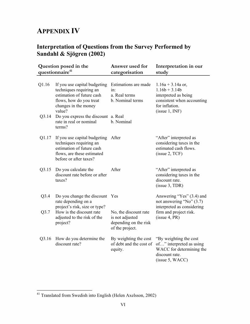
VI
APPENDIX IV Interpretation of Questions from the Survey Performed by Sandahl & Sjögren (2002) Question posed in the questionnaire41
Answer used for categorisation
Interpretation in our study
Q1.16 If you use capital budgeting
techniques requiring an estimation of future cash flows, how do you treat changes in the money value?
Estimations are made in: a. Real terms b. Nominal terms
Q3.14 Do you express the discount rate in real or nominal terms?
a. Real b. Nominal
1.16a + 3.14a or, 1.16b + 3.14b interpreted as being consistent when accounting for inflation. (issue 1, INF)
Q1.17 If you use capital budgeting
techniques requiring an estimation of future cash flows, are these estimated before or after taxes?
After “After” interpreted as considering taxes in the estimated cash flows. (issue 2, TCF)
Q3.15 Do you calculate the
discount rate before or after taxes?
After “After” interpreted as considering taxes in the discount rate. (issue 3, TDR)
Q3.4 Do you change the discount
rate depending on a project’s risk, size or type?
Yes
Q3.7 How is the discount rate adjusted to the risk of the project?
No, the discount rate is not adjusted depending on the risk of the project.
Answering “Yes” (3.4) and not answering “No” (3.7) interpreted as considering firm and project risk. (issue 4, PR)
Q3.16 How do you determine the
discount rate? By weighting the cost of debt and the cost of equity.
“By weighting the cost of…” interpreted as using WACC for determining the discount rate. (issue 5, WACC)
41 Translated from Swedish into English (Helen Axelsson, 2002)

VII
Q3.17 Which interest rate is used for determining the cost of debt?
The market interest rate for a corresponding loan.
“The market interest…” interpreted as using the market cost of debt (issue 5a, Market cost of debt)
Q3.18 How is the cost of equity
determined? CAPM or a similar volatility method.
“CAPM or a…” interpreted as using CAPM for determining the cost of equity. (issue 5b, CAPM)
Q3.19 How are the capital shares
determined in weighting debt and equity?
Market values of debt and equity
“Market values…” interpreted as using the market values of debt and equity (issue 5c, Market values)

VIII
APPENDIX V Questionnaire Please tick only one box for each question. If you have extra comments, please leave them to the end of the questionnaire. A. Please assign the capital appraisal techniques presented below a number between 1 and 5 depending on their degree of capital budgeting sophistication, where 1 is not at all sophisticated and 5 is very sophisticated.
1 2 3 4 5 1. Net present value (NPV) 2. Internal rate of return (IRR) 3. Simple payback period 4. Discounted payback period 5. Accounting ratio (Rt, ROI, ROE, ROCE etc)
The following sections focus on issues related to the application of discounted cash flow techniques B. Please assign a number between 1 and 5 depending on the importance of the issues in question, where 1 is not at all important and 5 is very important.
1 2 3 4 5 1. Consideration of taxes when estimating the expected cash flows.
2. Consideration of taxes when estimating the discount rate.
3. Consideration of firm risk and project/divisional risk.
C. Please assign a number between 1 and 5 depending on the importance of the issue, where 1 is not at all important and 5 is very important. 1 2 3 4 5 1. Consistency when accounting for inflation i.e., real cash flows are discounted by a real discount rate and nominal cash flows are discounted by a nominal discount rate.
D. How does the method for determining the discount rate affect a firm’s capital budgeting sophistication? Assign the methods presented below a number between 1 and 5 depending on their degree of sophistication, where 1 is not at all sophisticated and 5 is very sophisticated.
1 2 3 4 5 1. Discount rate commonly used within the firm/ industry
2. Borrowing rate 3. Opportunity cost 4. The weighted average cost of capital (WACC) 5. Calculation based on the P/E ratio 6. Borrowing rate plus a risk premium

IX
E. Assume WACC is used when estimating the discount rate, how important do you consider the following issues? Please assign a number between 1 and 5 depending on the importance of the issue in question, where 1 is not at all important and 5 is very important.
1 2 3 4 5 1. The cost of debt determined as the market interest rate for equivalent loans.
2. The cost of equity determined by using the capital asset pricing model (CAPM).
3. The value of equity and debt estimated in terms of market values.
The following sections deals with the whole capital budgeting process F. Please assign the phases in the capital budgeting process as presented below a number between 1 and 5 depending on their importance for the firm’s capital budgeting sophistication, where 1 is not at all important and 5 is very important.
1 2 3 4 5 1. Determination of an investment budget 2. Identification i.e., the search and identification of projects
3. Development i.e., screening and definition of projects
4. Evaluation i.e., project appraisal and decision choice
5. Implementation 6. Control and post-audits
G. How far do you agree to our assertion that the following activities and procedures are important when determining the sophistication of a firm’s investment process? Please assign a number between 1 and 5 to each activity, where 1 is I strongly disagree and 5 is I strongly agree. 1 2 3 4 5 1. The establishment of a long-term (> 2 years) capital budget.
2. The existence of a formal process for searching and identifying investment opportunities that are in accordance with the firm’s strategic goals.
3. Rewards to individuals who suggest good investments.
4. The existence of a formal process for screening investments proposals, where weak proposals are sorted out.
5. The definition of a number of alternative options for each proposal.
6. Applying a formal financial evaluation of investment proposals using DCF techniques and a risk adjusted required rate of return.
7. The establishment of an implementation plan and the assignment of a project manager when the

X
investment decision is made. 8. The application of regular and pre-agreed upon procedures for post-audits on the majority of investment projects.
9. The application of discounted cash flow techniques in post-auditing.
10. The results from post-audits are used to evaluate projects and to improve future forecasts.
11. Consideration of a project’s strategic aspects throughout the entire capital budgeting process.
Do you think that any important activities are missing? Please, describe them below:
Comments:

XI
APPENDIX VI Additional Information Concerning Answers Received from Academics Figure 11 NPV – Distribution Sophistication Scores
Figure 12 IRR –Distribution Sophistication Scores
NPV
012345
1 2 3 4 5 6 7 8 9 10
Respondents
Soph
istic
atio
n Sc
ore
Average Score: 4
IRR
012345
1 2 3 4 5 6 7 8 9 10
Respondents
Soph
istic
atio
n Sc
ore
Average Score: 3,7

XII
Figure 13 DPB – Distribution Sophistication Scores
Figure 14 ARR – Distribution Sophistication Scores
Discounted Payback (DPB)
012345
1 2 3 4 5 6 7 8 9 10
Respondents
Soph
istic
atio
n Sc
ore
Average Score: 2,3
ARR
012345
1 2 3 4 5 6 7 8 9 10
Respondents
Soph
istic
atio
n Sc
ore
Average Score: 2,2

XIII
Figure 15 PB – Distribution Sophistication Scores
Figure 16 Determination of the Discount Rate
Payback (PB)
012345
1 2 3 4 5 6 7 8 9 10
Respondents
Soph
istic
atio
n Sc
ore
Average Score: 1,4
Determination of the Discount Rate
2,2
2,6
2,9
3
3,2
3,5
0 1 2 3 4 5
Calculation based on the P/E ratio
Borrowing rate
Discount rate commonly used withinthe firm/industry
Borrowing rate plus a risk premium
WACC
Opportunity cost
Average Score

XIV
Figure 17 Stages in the Capital Budgeting Process
Comments – Activities that according to the respondents should be included when defining the capital budgeting process (literally presented): Comparison to investment decisions by competitors. Human resources as investment. Information to shareholders in annual reports and interim reports.
Stages in the Capital Budgeting Process
3,8
3,8
4,4
4
4,1
3,7
0 1 2 3 4 5
Control and post-audits
Implementation
Evaluation
Development
Identification
Investment budget
Average Score

XV
APPENDIX VII Theoretical Description - Tests of Regression Assumptions and Significance Tests Testing Homoskedasticity (Assumption 3) According to Hill et al (2001) there are two ways of discovering heteroscedasticity, i.e., when the variances of all observations are not the same. One method is to plot the least square residuals against an explanatory variable. If no patterns of any kind can be seen, the assumption of homoskedasticity can be considered valid. In order to discover heteroskedasticity in the case of a multiple regression, residuals should be plotted against each explanatory variable, which demands a great effort. Besides, this method cannot be used to define whether variations in the magnitude of the residuals produce statistical evidence against homoskedasticity. The Goldfeld-Quandt test is therefore suggested to test the assumption about homoskedasticity. In order to perform the test, the sample is divided into two sub-samples with n1 and n2 observations in such a way that under the null hypothesis of homoskedasticity H0: σ2
1=σ22, the variances would be the same
in the two groups, but under the alternative hypothesis, the variances of the observations would differ systematically H1: σ2
1=σ2xt. Then for each sub-sample the estimated error variances are estimated, 2
1σ̂ and 22σ̂ (denoted MS
Residual in Excel). The Goldfeld-Quandt (GQ) test statistic is estimated as follows:
)(ˆ)(ˆ
222
121
KnKnGQ
−−
=σσ
Equation 31 The Goldfeld-Quandt Test Statistic
where the larger disturbance is assumed to be in the first sample (Greene, 1997; Hill et al, 2001). Under the null hypothesis of homoskedasticity GQ statistic has an F-distribution with (n1–K) and (n2–K) degrees of freedom, where K is the number

XVI
of parameters in the regression model. Hence, if the GQ statistic exceeds the critical value of Fc with a chosen degree of significance, e.g.,, 0.05, the null hypothesis of homoskedasticity is rejected in favour of heteroskedasticity (Greene, 1997). Testing Autocorrelation (Assumption 4)
In order to introduce the Durbin-Watson test for autocorrelation, the errors of the linear regression model are assumed to be represented by the following model: et = ρ42 et-1 + νt
Equation 32 Errors of the Linear Regression Model
where νt are independent random errors with distribution N(0, 2
νσ )(Hill et al, 2001). If ρ=0, then et-1=νt and errors in the linear regression model are not autocorrelated. Hence, the null hypothesis of no autocorrelation is H0: ρ=0 against the alternative H1: ρ>0. The Durbin-Watson statistic d is then calculated using the following formula:
∑
∑
=
=−−
= T
tt
T
ttt
e
eed
1
2
2
21
ˆ
)ˆˆ(
Equation 33 The Durbin-Watson Test Statistic
The d statistic can be expressed approximately as d=2(1- ρ̂ ). Hence, if ρ=0, then d≈2, indicating no autocorrelation, and if ρ̂ =1, then d≈0 and the errors are correlated. This test is however not precise enough to determine where in the interval between 0 and 2 the d statistic should be to conclude about no autocorrelation. This problem can be solved using either the critical value of d distribution or the bond test. The following decision rule can be used under the bond test:
42 ρ is a parameter that determines the correlation properties of et. (Hill et al, 2001).

XVII
If d < dLc, hence, reject H0 and accept H1 If d > dUc, do not reject H0 If dLc < d < dUc , the test is inconclusive
Values of dLc and dUc can be obtained from the statistical tables for the chosen level of significance (Hill et al, 2001).
Testing Collinearity (Assumption 5)
Collinearity can be detected using two methods (Hill et al, 2001). One of the methods is a correlation analysis. In this case one can assume that a correlation coefficient between two explanatory variables larger than 0.8 or 0.9 in absolute value indicate a strong linear and, thus, a potentially collinear relationship. The drawback of this method is its inability to capture the collinearity relationship involving more than two explanatory variables. Hence, another procedure is proposed which is referred to as “auxiliary regressions”. It involves estimating a regression model where one of the explanatory variables becomes a dependent variable and all other explanatory variables are independent variables. Looking at the coefficient of determination (R2 > 0.8), one can conclude about existence of collinearity between explanatory variables (Ibid). Potential impediment the use of the latter method lies in the large amount of effort required for testing all combinations of explanatory variables in case of multiple regression. Testing Normality in Distribution of Residuals (Assumption 6)
When choosing a functional form, it is desirable that in the created model errors are normally distributed. The Jarque-Bera test is a formal test that allows to analyse whether residuals come from a normal distribution. It is based on two measures, skewness and kurtosis, where skewness (S) shows how symmetric the residuals are distributed around their mean value equal to 0 and kurtosis (K) refers to “peakedness” of the distribution which is equal to 3 for a normal distribution.

XVIII
The Jarque-Bera statistic is estimated by the following formula:
−+=
4)3(
6
22 KSTJB
Equation 34 The Jarque-Bera Test Statistic
It is then compared to the critical value of the chi-squared distribution with K degrees of freedom. If the JB-statistic exceeds the critic value, the null hypothesis about normally distributed errors is rejected (Hill et al, 2001). Testing the Significance of a Single Coefficient, t-test In order to find out whether the dependent variable is related to an explanatory variable, the “test of significance” for a single variable is accomplished. If the tested variable has no effect on the explanatory variable, then the true beta of this explanatory variable is equal to zero (βk=0). In order to control for it, the null hypothesis H0: βk=0 is tested against the alternative H1: (βk≠0). The H0 is rejected, implying that the tested variable is significant, if the computed value of the test statistic (t-statistic) falls in the rejection region, i.e., t-statistic ≥ tc or t-statistic ≤ -tc, where tc is the critical value from t-distribution with (T-K) degrees of freedom. The t-statistic is calculated as follows:
)( k
k
bseb
t =
Equation 35 The t-test Statistic
where se(bk) is a standard error of bk. The critical value tc varies depending on the level of significance chosen (0.01 or 0.05). If the dependent variable is not related to the tested explanatory variable then the null hypothesis cannot be rejected (Hill et al, 2001). The Excel function can be used for the t-test, as both the t-statistic and the critical value are provided. Moreover, Excel also provides a p-value, which shows the

XIX
probability that the t-distribution (tc) can take a value greater than or equal to the absolute value of the sample value of t-statistic. When the p-value is smaller than the chosen value of the level of significance (0.01 or 0.05), then the null hypothesis is rejected (Hill et al, 2001). Testing the Significance of the Model, F-test
The overall significance of a model is being tested in the multiple regression model using the F-test. For a regression model with K-1 explanatory variables, the null hypothesis H0: β2=0, H0: β3=,.., βk=0 against the alternative, H1: “at least one of the βk is nonzero”. If the null hypothesis is true, none of the variables influence the dependent variables and the model has little or no value. If the alternative hypothesis is true, then at least one of the explanatory variables has influence of the dependent variables (Hill et al, 2001). In order to test these hypotheses, the F-test statistic is calculated as follows:
)/()1/()(
KTSSEKSSESSTF
−−−
=
Equation 36 The F-test Statistic
where T is a number of observations and K is a number of regression parameters. It is then compared to the critical value from the F(K-1, T-K) distribution. If the F-statistic exceeds the critical Fc value at the chosen level of significance, the null hypothesis is rejected and the model is assumed to be significant. Similar to t-test Excel provides a p-value also for the F-test. The conclusion to reject the hull hypothesis can be made if the estimated p-value is smaller the chosen level of significance (Ibid).

CA
PIT
AL
BU
DG
ET
ING
SO
PHIS
TIC
AT
ION
AN
D P
ER
FOR
MA
NC
E
C
HA
PTE
R 8
XX
APP
EN
DIX
VII
I C
orre
latio
n M
atri
x - L
arge
Sam
ple,
Mod
el I
Tab
le 7
Cor
rela
tion
Mat
rix –
Lar
ge S
ampl
e, M
odel
I
NPV
IR
R
DPB
A
RR
PB
C
BS
Def
IL
n Si
zeR
isk
SDC
apita
l In
tens
ityL
ever
age
1997
L
n Si
ze
0.14
35
0.29
17-0
.197
1-0
.028
4-0
.171
0 0.
2798
1
O
RR
Adj
-0
.166
8-0
.054
9-0
.153
90.
0506
0.33
13
-0.2
659
0.25
31
-0.1
399
-0.0
303
-0.0
892
1998
L
n Si
ze
0.12
63
0.29
82-0
.191
5-0
.037
5-0
.153
7 0.
2633
1
O
RR
Adj
-0
.081
0-0
.120
6-0
.062
50.
1441
0.12
66
-0.1
557
0.23
96
-0.3
301
-0.0
229
-0.1
118
1999
L
n Si
ze
0.15
37
0.28
83-0
.195
1-0
.071
9-0
.150
2 0.
2803
1
O
RR
Adj
-0
.059
00.
0333
-0.1
067
0.09
640.
0698
-0
.060
0 0.
2990
-0
.286
0-0
.029
7-0
.018
6 20
00
Ln
Size
0.
1486
0.
2724
-0.1
767
-0.0
981
-0.1
304
0.26
43
1
OR
RA
dj
-0.0
331
0.12
37-0
.018
30.
0697
-0.0
814
0.04
73
0.14
65
-0.0
124
-0.0
786
-0.1
703
2001
L
n Si
ze
0.13
72
0.27
33-0
.174
0-0
.086
9-0
.128
5 0.
2549
1
O
RR
Adj
0.
0297
-0
.041
0-0
.099
60.
1451
-0.0
245
0.01
19
0.21
69
-0.6
635
0.04
93
0.00
77
L
n Si
ze
0.14
93
0.28
42-0
.190
5-0
.068
8-0
.148
7 0.
2748
1
A
vera
ge P
erio
d 19
97-2
001
OR
RA
dj
-0.0
681
-0.0
217
-0.1
116
0.13
470.
0942
-0
.097
2 0.
2845
-0
.407
4-0
.042
1-0
.058
9

XX
I
Cor
rela
tion
Mat
rice
s - S
mal
l Sam
ple,
Mod
el I
Tab
le 8
Cor
rela
tion
Mat
rix –
Sm
all S
ampl
e, M
odel
I, 1
997-
1999
N
PV
IRR
D
PB
A
RR
PB
C
BS
Def
I L
n Si
ze
Ris
k SD
R
isk
be
ta
Cap
ital
Inte
nsity
Lev
erag
e19
97
Ln
Size
- 0
.076
0
0.39
05
- 0.2
083
- 0
.049
1
- 0.2
789
0.
1766
1
O
RR
Adj
- 0.1
481
- 0
.114
4
- 0.2
689
- 0
.039
9
0.32
90
- 0.3
400
0.
4057
0.
0208
- 0
.244
9
- 0.1
856
0.
1366
O
RR
- 0
.168
0
- 0.1
124
- 0
.218
3
- 0.0
537
0.
3160
- 0
.352
1
0.37
61
0.02
59
- 0.2
590
- 0
.203
1
0.12
89
∆ M
V Ad
j - 0
.135
6
- 0.0
328
- 0
.093
6
- 0.0
232
0.
1326
- 0
.210
3
- 0.0
915
- 0
.219
9
- 0.2
443
- 0
.282
0
0.23
16
∆ M
V
- 0.1
013
- 0
.049
2
- 0.0
717
- 0
.014
5
0.09
08
- 0.1
774
- 0
.030
2
- 0.0
855
- 0
.116
6
- 0.2
178
0.
1960
1998
L
n Si
ze
- 0.0
926
0.
4148
- 0
.198
5
- 0.0
636
- 0
.295
0
0.17
68
1
OR
R Ad
j - 0
.205
7
- 0.2
222
- 0
.043
5
0.04
71
0.20
79
- 0.4
179
0.
3619
- 0
.085
1
- 0.1
864
- 0
.568
3
0.37
52
OR
R
- 0.2
476
- 0
.214
8
0.09
61
0.01
22
0.15
80
- 0.4
342
0.
3103
- 0
.060
9
- 0.1
752
- 0
.585
7
0.36
27
∆ M
V Ad
j - 0
.271
6
- 0.0
246
0.
1450
- 0
.078
7
0.00
59
- 0.3
138
0.
0173
- 0
.128
5
- 0.2
352
- 0
.240
1
- 0.0
521
∆ M
V
- 0.2
257
0.
2017
- 0
.075
5
0.04
01
- 0.1
713
- 0
.095
6
0.44
14
0.21
38
- 0.0
012
- 0
.224
3
0.00
57
1999
L
n Si
ze
- 0.0
274
0.
4078
- 0
.191
9
- 0.1
015
- 0
.256
4
0.23
68
1
OR
R Ad
j - 0
.288
5
0.09
09
- 0.1
575
- 0
.071
3
0.26
43
- 0.3
086
0.
4869
- 0
.214
8
- 0.2
565
- 0
.426
5
0.13
99
OR
R
- 0.4
240
0.
1947
0.
0767
- 0
.162
0
0.19
14
- 0.3
418
0.
4621
- 0
.135
3
- 0.2
432
- 0
.437
2
0.13
64
∆ M
V Ad
j 0.
1028
- 0
.077
8
0.34
92
- 0.3
958
- 0
.087
2
0.03
45
- 0.3
934
- 0
.051
2
0.03
77
0.49
70
- 0.2
467
∆ M
V
- 0.0
666
- 0
.155
7
0.39
69
- 0.4
555
0.
2052
- 0
.226
9
- 0.2
152
0.
1342
0.
3356
0.
1351
- 0
.080
4

XX
II
Tab
le 9
Cor
rela
tion
Mat
rix –
Sm
all S
ampl
e, M
odel
I, R
emai
ning
Yea
rs
N
PV
IRR
D
PB
AR
R
PB
CB
S D
ef I
Ln
Size
Ris
k SD
Ris
k be
ta
Cap
ital
Inte
nsity
Lev
erag
e20
00
Ln
Size
-0
.018
9 0.
3720
-0
.183
8-0
.114
2-0
.208
40.
2152
1
OR
RA
dj
-0.0
814
0.26
50
-0.3
673
-0.0
527
0.25
13
0.02
57
0.36
92
0.33
83
0.19
10
0.05
19
-0.0
366
OR
R
-0.1
339
0.32
01
-0.1
270
-0.1
160
0.14
84
0.05
46
0.17
27
0.40
70
0.23
52
0.03
40
-0.1
301
∆M
VA
dj
-0.0
681
0.21
45
0.30
62
-0.2
838
0.07
60
0.10
35
0.32
80
0.13
86
0.27
21
-0.1
803
0.00
07
∆M
V
-0.0
803
0.23
69
-0.0
520
-0.1
169
0.11
81
0.06
40
0.62
45
0.27
66
0.63
06
-0.0
413
-0.0
016
2001
L
n Si
ze
-0.0
273
0.37
00
-0.1
869
-0.1
130
-0.2
177
0.20
36
1
O
RR
Adj
-0
.106
4 -0
.102
5-0
.054
00.
1188
0.
0297
-0
.188
9 0.
0309
-0
.662
5-0
.574
7-0
.376
9 0.
0884
O
RR
-0
.164
3 0.
0467
-0
.022
00.
0662
-0
.067
4-0
.135
7 -0
.028
6-0
.646
0-0
.695
5-0
.288
5 0.
0415
∆
MV
Adj
0.
1015
0.
0907
0.
1472
0.
1383
-0
.352
40.
2630
0.
3018
0.
1057
0.
0586
-0
.201
9 0.
0415
∆
MV
0.
1603
-0
.047
80.
1674
-0
.144
4-0
.074
80.
1456
0.
1860
0.
0837
-0
.109
3-0
.281
9 0.
1242
Ln
Size
-0
.035
9 0.
3922
-0
.199
1-0
.096
1-0
.241
10.
2137
1
O
RR
Adj
-0
.218
1 -0
.030
7-0
.236
30.
0029
0.
2871
-0
.330
4 0.
4197
-0
.166
4-0
.293
5-0
.441
0 0.
2413
A
vera
ge
Perio
d 19
97-2
001
OR
R
0.13
41
-0.0
497
0.05
16
-0.4
994
0.22
47
-0.0
063
0.07
67
0.01
74
-0.1
474
0.11
66
-0.5
317
∆M
VA
dj
-0.1
141
0.09
61
0.43
99
-0.3
225
-0.1
418
-0.0
252
0.01
46
-0.0
855
-0.0
563
-0.0
610
0.03
86
∆M
V
-0.1
144
0.10
16
0.11
31
-0.2
804
0.09
85
-0.0
899
0.43
17
0.26
44
0.36
25
-0.2
561
0.13
12

CAPITAL BUDGETING SOPHISTICATION AND PERFORMANCE CHAPTER 8
XXIII
APPENDIX IX Empirical Tests of Regression Assumptions Each regression model must be carefully examined to confirm that the assumptions of the regression model are valid. If the assumptions are not valid the least square procedure may not be very effective (Hill et al, 2001). It is important to make sure that the regression assumptions are fulfilled if one intends to generalise findings to the population, from which the sample was drawn. Several tests have been conducted for the regression equations performed on the large sample in order to evaluate the quality of the findings obtained. The results are presented in Table 7.
Table 10 Tests of Regression Assumptions - Large Sample
F = Fulfilled Assumption N/F = Not Fulfilled (3) Assumption 3 of homoskedasticity is fulfilled for 1997 and violated for the period 1998-2001 and the average period. The violation results in regression estimates that are still linear and unbiased, but are no longer the best (BLUE) estimators. This may lead to incorrectly computed standard errors for the least square estimators. Therefore, the significance tests for the individual regression coefficients may be misleading. (Hill et al, 2001). (4) The assumption of no autocorrelation is fulfilled for the whole period 1997-2001 and the average period.
Assumption Test 1997 1998 1999 2000 2001Average
1997-20013 GQ (p-value) 0,9890 0,0000 0,0019 0,0003 0,0076 0,0000
Result F N/F N/F N/F N/F N/F4 d-statistic 1,97 2,35 2,28 2,10 2,06 2,14
Result F F F F F F5 Result F F F F F F6 JB (p-value) 0,5024 0,0566 0,0000 0,0024 0,0093 0,0226
Result F F N/F N/F N/F N/F

XXIV
(5) No correlation coefficients exceeding the control value of 0.8 have been found for the whole period 1997-2001 and the average period, implying that Assumption 5 is also fulfilled.
(6) Assumption 6 is fulfilled for 1997 and 1998 and violated for the period 1999-2001 and for the average period. The fact that Assumption 6 is violated questions inferences drawn from the regression equations since both F-statistics and t-statistics are adversely affected. Based on the above tests, one can conclude that all the regression assumptions are fulfilled in the regression model for 1997 and the results can be generalised. For the regression model in 1998 the assumption of homoskedasticity is not fulfilled, hence, the estimated regression coefficients for the CBS variable and explanatory variables should be treated with caution. For the remaining regression equations (1999-2001 and the average period) Assumption 3 and 6 are not fulfilled. Since both assumptions are to a large extent related to hypothesis testing, both for the individual coefficients and for the whole model, these results impose serious restrictions on the significance tests.