cantera integration with the toolbox for modeling and ... integration with the toolbox for modeling...

American Institute of Aeronautics and Astronautics

1

Cantera Integration with the Toolbox for Modeling and Analysis of Thermodynamic Systems (T-MATS)

Thomas M. Lavelle1 NASA Glenn Research Center Cleveland, Ohio 44135

Jeffryes W. Chapman2 Vantage Partners, LLC, Brook Park, Ohio 44142

Ryan D. May3 Vantage Partners, LLC, Brook Park, Ohio 44142

Jonathan S. Litt4 and Ten-Huei Guo5 NASA Glenn Research Center Cleveland, Ohio 44135

NASA Glenn Research Center (GRC) has recently developed a software package for modeling generic thermodynamic systems called the Toolbox for the Modeling and Analysis of Thermodynamic Systems (T-MATS). T-MATS is a library of building blocks that can be assembled to represent any thermodynamic system in the Simulink® (The MathWorks, Inc.) environment. These elements, along with a Newton Raphson solver (also provided as part of the T-MATS package), enable users to create models of a wide variety of systems. The current version of T-MATS (v1.0.1) uses tabular data for providing information about a specific mixture of air, water (humidity), and hydrocarbon fuel in calculations of thermodynamic properties. The capabilities of T-MATS can be expanded by integrating it with the Cantera thermodynamic package. Cantera is an object-oriented analysis package that calculates thermodynamic solutions for any mixture defined by the user. Integration of Cantera with T-MATS extends the range of systems that may be modeled using the toolbox. In addition, the library of elements released with Cantera were developed using MATLAB native M-files, allowing for quicker prototyping of elements. This paper discusses how the new Cantera-based elements are created and provides examples for using T-MATS integrated with Cantera.

Nomenclature

CEA = Chemical Equilibrium Analysis C-MAPSS 40k = Commercial Modular Aero-Propulsion System Simulation, 40k JANAF = Joint Army, Navy, Air Force NPSS = Numerical Propulsion System Simulation T-MATS = Toolbox for the Modeling and Analysis of Thermodynamic Systems

1 Aerospace Engineer, 21000 Brookpark Rd., 2 Aerospace Engineer, 21000 Brookpark Rd. AIAA Member 3 Electrical Engineer, 21000 Brookpark Rd., AIAA Member 4 Control Systems Engineer, 21000 Brookpark Rd., MS 77-1, AIAA Senior Member 5 Control Systems Research Engineer, 21000 Brookpark Rd., MS – 77-1, AIAA Member

https://ntrs.nasa.gov/search.jsp?R=20150000137 2018-07-08T09:55:12+00:00Z


2

I. Introduction VER the past several years, NASA GRC has been developing MATLAB/Simulink-based methods for modeling thermodynamic systems. The most recent iteration of work has resulted in the Commercial Modular Aero-

Propulsion System Simulation, 40k (C-MAPSS 40k) engine model. With a little effort, it was possible to adapt this specialized engine model into a more general, open source Simulink modelling framework. Known as the Toolbox for Modeling and Analysis of Thermodynamic Systems (T-MATS),1 this development represents a major step forward in the area of thermodynamic simulations as it allows the user to model thermodynamics systems in any configuration, using elements from the T-MATS library. Contained in this library are models of turbomahcinery and other mechanical components required to simulate systems such as high-bypass and turbofan engines. The T-MATS package uses tabular lookup for combustion properties of air, humidity, and a hydrocarbon fuel, which may be made more flexible through integration with the Cantera thermodynamic package.

Cantera is an object-oriented thermodynamic package that can be used to calculate the thermodynamics, kinetics, and transport properties of any flow.2 (Cantera can be obtained from the Cantera project web-site. It is currently released under a BSD 3-c License agreement.) The thermodynamic properties of the species of interest are read from text input files, similar to how inputs are handled by the NASA Chemical Equilibrium Analysis (CEA) package.3 Since the Cantera files can be managed at run time, the chemical solution for the problem can be as simple or as complex as the user desires. Communication between Simulink and Cantera is handled through MATLAB functions that are part of the T-MATS Cantera release.

In addition to providing a mechanism for interfacing with Cantera, the T-MATS Cantera package includes a set of engineering components forming a baseline library for model development. This library contains blocks for all the components required to build a separate flow turbofan model and are written using the MATLAB M-file format. The M-file format enables quick prototyping since the code does not need to be compiled. Thermodynamic information is passed between elements using a specially-formatted data arrays.

The details of how Cantera can be integrated with T-MATS are presented in Section II and the creation of library blocks, based on M-functions, is detailed in Section III. The use of these blocks to construct a model using T-MATS Cantera is described in SectionIV, followed by example applications in a turbofan model and fuel cell model in Sections V and VI.

II. Cantera Integration In order to integrate Cantera with T-MATS, the MATLAB Cantera package must be installed to give the user

access to several built-in functions and scripts for creating flow models. These scripts will be introduced and discussed in this section as the interface with Cantera through MATLAB (and, by extension, T-MATS) is presented.

The first step in creating a simulation is to define the reactants in the system. Reactants are mixes of compounds that are created by different flow start elements. The script canterload.m contains the Name and Species arrays that define these reactants. For example, the lines:

Species = { .7547 .232 .0128 0 0 0;1 0 0 0 0 0; 1.0 0 0 0 0 0; 1 0 0 0 0 0; 0 0 0 0 0 0; 0 0 0 0 0 0}; Name = { 'N2' 'O2' 'AR' '' '' ''; 'H2' '' '' '' '' ''; 'H2O' '' '' '' '' ''; 'O2' '' '' '' '' ''; '' '' '' '' '' ''; '' '' '' '' '' '' }

define four reactants for a model: air (a mixture containing 75.47% N2, 23.2% O2, and 1.28% AR), H2, H2O, and O2. In addition to defining the composition of the reactants, an object has to be created in MATLAB to interface with Cantera. This is done in two steps, first by creating the global variable fs (the variable name expected by the T-MATS Cantera scripts) and then by defining the object contents using the Cantera command importPhase: fs = importPhase( 'gri30.xml' );

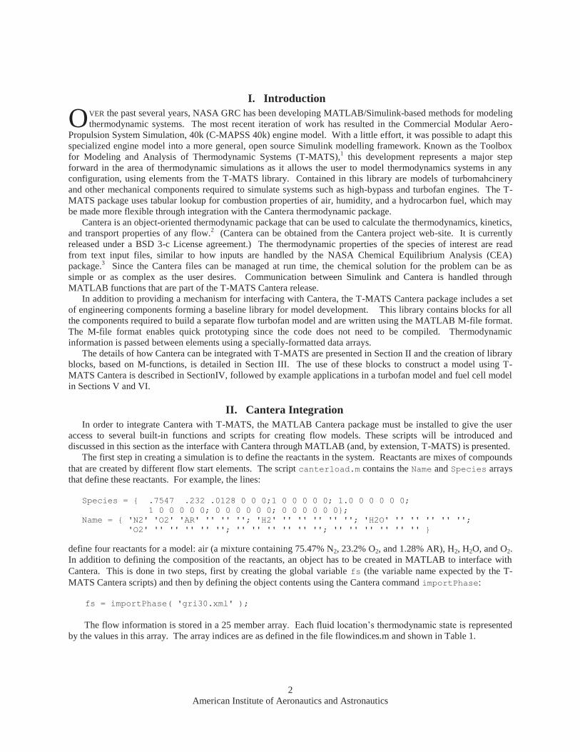
The flow information is stored in a 25 member array. Each fluid location’s thermodynamic state is represented

by the values in this array. The array indices are as defined in the file flowindices.m and shown in Table 1.

O


3

Table 1: Structure of the flow arrays used by Cantera.

Information Index Description W 1 Weight of the flow Tt 2 Total temperature Pt 3 Total pressure Ht 4 Total enthalpy comp1 (to) comp10 5-14 Percentage of flow composition for reactants 1 to 10 S 15 Entropy Rhot 16 Total density Ts 17 Static temperature Ps 18 Static pressure Hw 19 Static enthalpy Rhos 20 Static density Vflow 21 Flow velocity MN 22 Flow Mach number A 23 Flow area Gamt 24 Total gamma Gams 25 Static gamma

Each piece of flow information may be indexed directly, or using the variable name; for example, static density of a location Fl_in would be referenced as Fl_in(20) or Fl_in(rhos) .

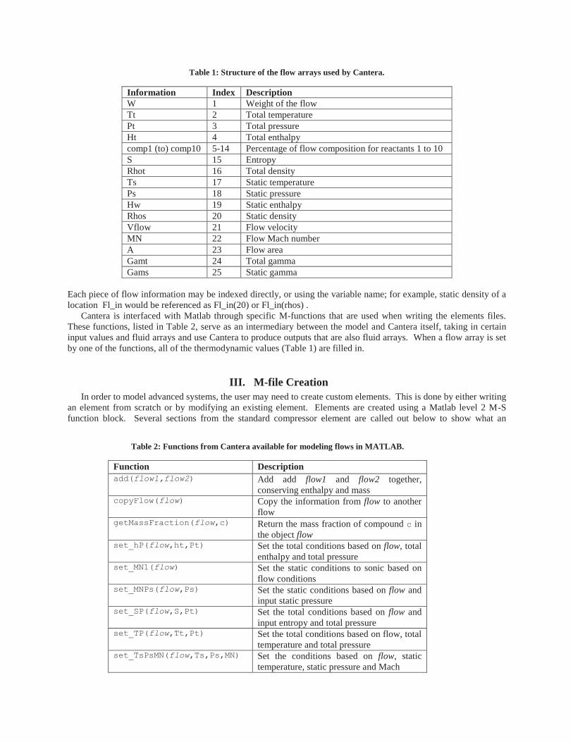
Cantera is interfaced with Matlab through specific M-functions that are used when writing the elements files. These functions, listed in Table 2, serve as an intermediary between the model and Cantera itself, taking in certain input values and fluid arrays and use Cantera to produce outputs that are also fluid arrays. When a flow array is set by one of the functions, all of the thermodynamic values (Table 1) are filled in.

III. M-file Creation In order to model advanced systems, the user may need to create custom elements. This is done by either writing

an element from scratch or by modifying an existing element. Elements are created using a Matlab level 2 M-S function block. Several sections from the standard compressor element are called out below to show what an

Table 2: Functions from Cantera available for modeling flows in MATLAB.

Function Description add(flow1,flow2) Add add flow1 and flow2 together,

conserving enthalpy and mass copyFlow(flow) Copy the information from flow to another

flow getMassFraction(flow,c) Return the mass fraction of compound c in

the object flow set_hP(flow,ht,Pt) Set the total conditions based on flow, total

enthalpy and total pressure set_MN1(flow) Set the static conditions to sonic based on

flow conditions set_MNPs(flow,Ps) Set the static conditions based on flow and

input static pressure set_SP(flow,S,Pt) Set the total conditions based on flow and

input entropy and total pressure set_TP(flow,Tt,Pt) Set the total conditions based on flow, total

temperature and total pressure set_TsPsMN(flow,Ts,Ps,MN) Set the conditions based on flow, static

temperature, static pressure and Mach


4

engineer needs to do in order to modify/create their own element. Somewhere in the M-file, the user will have to create ports that enable data to flow from one element to another.

The two sections of code provided below show this for two ports of the compressor block. The first port is the primary incoming flow. This port is an array of 25 variables, matching the size of the fluid array. The second section shows a single-variable data port that is used to take the value of mechanical speed and pass it into a local variable. Output ports are managed in the same way.

% incoming flow block.InputPort(1).Dimensions = 25; block.InputPort(1).DatatypeID = 0; % double block.InputPort(1).Complexity = 'Real'; block.InputPort(1).DirectFeedthrough = true; block.InputPort(1).SamplingMode = 'Sample'; FI = block.InputPort(1).Data;

% Override input port properties block.InputPort(2).Dimensions = 1; block.InputPort(2).DatatypeID = 0; % double block.InputPort(2).Complexity = 'Real'; block.InputPort(2).DirectFeedthrough = true; block.InputPort(2).SamplingMode = 'Sample'; Nmech = block.InputPort(2).Data;

Another source of data used in the calculations are the Simulink input dialog boxes that correspond to this

element. The example below shows how the input design efficiency is loaded into the compressor from the dialog panel.

effDes = block.DialogPrm(3).Data; One major issue in using Simulink for this type of modelling is the inability for each element to have its own

instances of each internal variable. To get around this issue, global variable names are created by using the gcb() command to get the object’s instance name. The functions setV() and getV() are used to take the object name, append the local variable to it, and write and retrieve it from the MATLAB global workspace. An example of setting and retrieving the speed scalar, s_C_Nc, is shown below.

path = stripchar( gcb() ); setV( 's_C_Nc', path, s_C_Nc ); s_C_Nc = getV( 's_C_Nc', path );

Another standard used by the elements in this package is the IDes variable. This variable determines how the

map scalars are used. When IDes = 0, the desired values for parameters such as efficiency and pressure ratio are supplied by the user. Map scalar values are calculated and stored in the MATLAB workspace for use in future simulations. For an IDes value of 1, scalar values are read from the workspace and used. For an IDes value of 2, scalars are provided directly by the user. The section below shows the different scaling values as determined for a compressor map.

if IDes < .5 s_eff = effDes / effMap; s_PR = ( PRdes - 1 )/( PRmap - 1 ); s_Wc = WcIn/ WcMap; setV( 's_eff', path, s_eff ); setV( 's_Wc', path, s_Wc ); setV( 's_PR', path, s_PR ); elseif IDes < 1.5 % get the maps scalars from the workspace s_eff= getV( 's_eff', path ); s_Wc= getV( 's_Wc', path ); s_PR= getV( 's_PR', path );


5

else % use the input values s_eff = s_eff_in; s_Wc = s_Wc_in; s_PR = s_PR_in; end

After the M-file code performs these preliminary tasks, it then executes a series of thermodynamic calculations. The code section below shows how the compressor determines the ideal state from the entropy and exit pressure, then determines the actual enthalpy from the ideal enthalpy, and finally sets the exit conditions based on the actual enthalpy and pressure.

FOideal = set_SP( FI, FI(s),PtOut ); htOut = FI(ht) + ( FOideal(ht) - FI(ht) )/eff; % set the exit conditions to knowm enthalpy and pressure FO = set_hP( FI, htOut, PtOut );

Once the code has been written, a mask may be created for the M-S function block to clearly specify the input

block parameters and add labels to the input and output ports. The first step in mask creation is to label all of the ports and, for consistency with other blocks in the T-MATS Cantera library, color code the port names. The standard colors used for T MATS are: blue for fluid ports, dark green for solver independent variable ports, green for solver dependent variable ports, and black for mechanical information. For the compressor, the drawing commands to produce the mask are shown in Figure 1.

Figure 1. Compressor element mask appearance settings.

After customizing how the block appears in the Simulink window, the user should provide descriptions for each

dialog parameter through the interface accessible under the “Parameters” tab of the Mask Editor. For every variable that appears in the M-S function dialog box, the mask definition should specify a description of the input (what appears in the mask) and a variable name for the input (used within the masked system). For the compressor, the filled-in “Parameters” tab can be seen in Figure 2.


6

Figure 2. Compressor Simulink mask variables.

Finally, the user must use the variable names for the parameters defined in the mask to specify the parameters of

the M-S function block, as shown in Figure 3. This window contains the S-function name that will be executed as well as all of the parameters that will be passed into the S-function. The parameter names must match the variable names defined in the parameter window of the mask editor in order to ensure the S-function is performing calculations with the correct information. Inside the S-function, they will be read off, in order, from the block.DialogPrm array.

Figure 3. Compressor Simulink S-function block parameters.

IV. Model Construction Once new elements have been created and added to the T-MATS Cantera Simulink library, the model may be

built and run following the same process as with T-MATS v.1.0.1; for more details, see the T-MATS user’s guide.1 The main difference between a model constructed using T-MATS v.1.0.1 and one using T-MATS Cantera is the extra fluid information available in the expanded flow vector.

V. Turbofan Example A model of a turbofan engine was constructed using T-MATS Cantera and compared to the same engine

modeled using the Numerical Propulsion System Simulation (NPSS) with the JANAF thermodynamic package. JANAF, like CEA and Cantera, is a thermodynamic equilibrium package that uses the same solution methods as


7

CEA, but is structured for a fixed product list and optimized for speed. It runs much quicker than CEA. For this example, the model is a version of the JT9D, one of the original 747 engines, which uses publically available data.4 . Figure 4 contains the block diagram showing how the model is implemented in Simulink using blocks from the T-MATS Cantera library.

Figure 4. T-MATS Cantera model of JT9D like engine.

Table 3. Comparisons of TMATS with NPSS.

NPSS with JANAF Output TMATS Cantera Output Altitude 34000 ft 34000 ft Mach number .8 .8 Weight flow 674 lbm/sec 674 lbm/sec Thrust 11194 lbf 11182 lbf SFC .6113 .6116

As can be seen from the results above (Table 3), the data matches up very well between the two models, indicating that the combination of Cantera and T-MATS is a viable option for thermodynamic modeling. The inclusion of Cantera enables T-MATS to model thermodynamic systems where hydrocarbon fuels are not used and/or air is not the oxidizer, such as the fuel cell in the next example.

VI. Fuel Cell Example

To show the advantages of the use of T-MATS Cantera in an application separate from engine model, a model of a simple fuel cell, based on previous NASA work,5 was constructed.


8

Figure 5. Simple solid oxide fuel cell model.

The details of the fuel cell model itself are not provided in this paper, but the model is available for download for those who wish to delve into it. Instead, several code snippets are shown to outline the implementation of the model, particularly those dealing with management of the reactants and removing reactants from the flow. The Simulink block diagram for this system is shown in Figure 5.

The section of code shown below appears near the beginning of the code to create a flow array Fl_tempH2, which has a composition of pure H2. It then sets the flow weight element of the array to the amount of hydrogen removed from the flow as it combines with oxygen to form water. Finally, the thermodynamic conditions are set to the anode temperature and pressure using the function set_TP().

Fl_tempH2(6) = 1; %set the composition to pure H2 Fl_tempH2(W) =-wH2_lost; Fl_tempH2 = set_TP( Fl_tempH2, Fl_Anode1(Tt), Fl_Anode1(Pt) );

Later in the code, output flow array Fl_O1 is created by adding the water and hydrogen flow arrays to the flow at the anode (array Fl_Anode2). Since the hydrogen flow is negative, Fl_O1 is the result of removing hydrogen from the flow and adding water back in. Fl_O1=add( Fl_Anode2, Fl_tempH2O ); Fl_O1=add( Fl_O1, Fl_tempH2 );

Additional calculations are represented by the final snipped of code provided below. Here, the fraction of oxygen in the cathode flow is determined using the function getcomp() and multiplied by the cathode flow weight to determine the mass flow of oxygen at the cathode.


9

%Gets total mass flow rate w_Cathode1 = Fl_Cathode1(W) * 453.; % g/sec xO2_Cathode1 = getcomp( Fl_Cathode1, 'O2' ); %Composition as mass flow (g/sec) xO2_Cathode1 = getcomp( Fl_Cathode1, 'O2' ); %Composition as mass flow (g/sec) wO2_Cathode1 = xO2_Cathode1 * w_Cathode1; The overall output for the fuel cell can be seen in the output display window highlighted in Figure 6. In this case, the electric power is 50kw, the cell voltage ideal is 1.075 V, the cell voltage operational is .6934 V, the efficiency of a cell stack is .93, the heat generated by the cell stack is 27.6 kW, the net heat output from the cell stack is 91.8 kw, the power density is .5727 W/cm2, and the weight flow of H2 used is .7547 grams/sec. Note that this fuel cell element can be used as part of a larger model, where the input and output flows interacts with components in a much larger system. Fox example, this fuel cell element can be used in larger simulations, such as a complete power plant for vehicle.

VII. Conclusion

Cantera has been integrated with the T-MATS package through the development of M-file-based library blocks modeling various thermodynamic elements. This combination greatly increases the capabilities and flexibility of the T-MATS package. Because T-MATS is now integrated with Cantera, engineers are no longer limited by the thermodynamics of pre-existing tables. This enables any thermodynamic flow to be modelled. In addition, creating a library of elements based on the Simulink M-file architecture allows engineers to quickly create new elements or modify existing ones, allowing quick prototyping of new systems. This was demonstrated both for

Figure 6. Solid oxide fuel cell output data.


10

a turbofan engine and for a fuel cell, but any thermodynamic flow can be modelled with any engineering element, allowing the engineer to create any type of advanced system.

References 1Chapman, J.W., Lavelle, T.M., May, R.D., Litt, J.S., Guo, T.H., “Toolbox for the Modeling and Analysis of

Thermodynamic Systems (T-MATS) User’s Guide,” NASA/TM-2014-216638, January 2014. 2D. Goodwin, "Cantera: An object-oriented software toolkit for chemical kinetics, thermodynamics, and

transport processes", Caltech, Pasadena, 2009. 3Gordon, S., and B.J. McBride, 1994: Computer Program for Calculation of Complex Chemical Equilibrium

Compositions and Applications. I. Analysis. NASA Reference Publication NASA RP-131, 1994. 4Chapman, J.W., Lavelle, T.M., May., Litt, J.S., Guo, T.H., “Toolbox for the Modeling and Analysis of

Thermodynamic Systems (T-MATS) User’s Guide,” A Process for the Creation of T MATS Propulsion System Models from NPSS data”, 2014.

5J. E. Freeh , C. J. Steffen Jr. and L. M. Larosiliere "Off-design performance analysis of a solid-oxide fuel cell/gas turbine hybrid for auxiliary aerospace power", Proc. FUELCELL2005, 3rd Int. Conf. Fuel Cell Science, Engineering and Technology, pp.23 -25, 2005.

cantera integration with the toolbox for modeling and ... integration with the toolbox for modeling...

Documents