can’t pay or won’t pay? unemployment, negative equity, … · naics dummy 5 0.20 0.40 0 1 arm...

Can’t Pay or Won’t Pay? Unemployment,

Negative Equity, and Strategic Default

ONLINE APPENDIX

Kristopher Gerardi∗

FRB AtlantaKyle Herkenhoff†

University of MinnesotaLee Ohanian‡

UCLA

Paul Willen§

FRB Boston

May 2017

∗[email protected]†[email protected]‡[email protected]§[email protected]

This appendix supplements the empirical analysis in “Can’t Pay or Won’t Pay? Unemploy-

ment, Negative Equity, and Strategic Default” by Gerardi, Herkenhoff, Ohanian, and Willen.

Below is a list of the sections contained in this appendix.

Contents

A.1 Comparison of Existing Measures of Strategic Default 2

A.2 PSID Consumption Data and TAXSIM 3

A.3 List of Control Variables 5

A.4 IV Details 6

A.5 Strategic Default with Assets 8

A.6 QRM Definitions of Strategic Default 9

A.7 Baseline Regressions with DTI 10

A.8 Income Changes and Non-Linearities 11

A.9 Robustness 17

A.10 Comparison of Default Rates in PSID and McDash/Equifax 21

A.11 Strategic Default Estimates using PSID-McDash/Equifax Weights 24

A.12 Unweighted Strategic Default Table 26

1

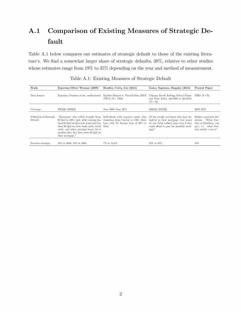
A.1 Comparison of Existing Measures of Strategic De-

fault

Table A.1 below compares our estimates of strategic default to those of the existing litera-

ture’s. We find a somewhat larger share of strategic defaults, 38%, relative to other studies

whose estimates range from 19% to 35% depending on the year and method of measurement.

Table A.1: Existing Measures of Strategic Default

Study Experian/Oliver Wyman (2009) Bradley, Cutts, Liu (2015) Guiso, Sapienza, Zingales (2013) Present Paper

Data Source: Experian (Number of obs. undisclosed) Equifax Merged w/ Payroll Data (EFXTWN) (N= 130k)

Chicago Booth Kellogg School Finan-cial Trust Index, Q4-2008 to Q3-2010,(N= 1k)

PSID (N=7k)

Coverage: 2004Q4–2009Q2 June 2008–June 2011 2008Q4–2010Q3 2009–2013

Definition of StrategicDefault:

“[b]orrowers who rolled straight from60 dpd to 180+ dpd, while staying lessthan 60 dpd on their auto loans and lessthan 90 dpd on their bank cards, retailcards, and other personal loans, for 6months after they first went 60 dpd ontheir mortgage.”

Individuals with negative equity whotransition from Current to 180+ DaysLate with No Income Loss of 20% orMore

Of the people you know who have de-faulted on their mortgage, how manydo you think walked away even if theycould afford to pay the monthly mort-gage?

Budget constraint def-inition: ”What frac-tion of defaulters ‘canpay’, i.e. what frac-tion satisfy c+m<y”

Fraction strategic: 19% in 2009, 18% in 2008 7% to 14.6% 25% to 35% 38%

2

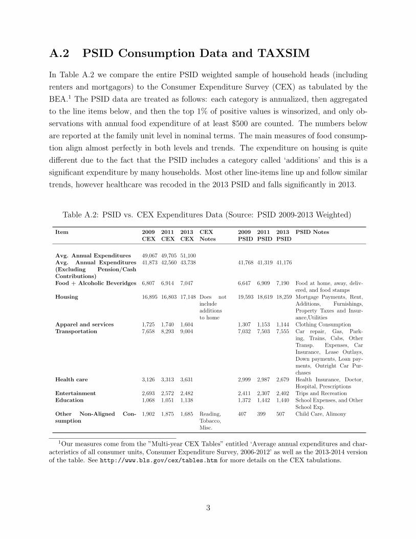
A.2 PSID Consumption Data and TAXSIM

In Table A.2 we compare the entire PSID weighted sample of household heads (including

renters and mortgagors) to the Consumer Expenditure Survey (CEX) as tabulated by the

BEA.1 The PSID data are treated as follows: each category is annualized, then aggregated

to the line items below, and then the top 1% of positive values is winsorized, and only ob-

servations with annual food expenditure of at least $500 are counted. The numbers below

are reported at the family unit level in nominal terms. The main measures of food consump-

tion align almost perfectly in both levels and trends. The expenditure on housing is quite

different due to the fact that the PSID includes a category called ‘additions’ and this is a

significant expenditure by many households. Most other line-items line up and follow similar

trends, however healthcare was recoded in the 2013 PSID and falls significantly in 2013.

Table A.2: PSID vs. CEX Expenditures Data (Source: PSID 2009-2013 Weighted)

Item 2009CEX

2011CEX

2013CEX

CEXNotes

2009PSID

2011PSID

2013PSID

PSID Notes

Avg. Annual Expenditures 49,067 49,705 51,100Avg. Annual Expenditures(Excluding Pension/CashContributions)

41,873 42,560 43,738 41,768 41,319 41,176

Food + Alcoholic Beveridges 6,807 6,914 7,047 6,647 6,909 7,190 Food at home, away, deliv-ered, and food stamps

Housing 16,895 16,803 17,148 Does notincludeadditionsto home

19,593 18,619 18,259 Mortgage Payments, Rent,Additions, Furnishings,Property Taxes and Insur-ance,Utilities

Apparel and services 1,725 1,740 1,604 1,307 1,153 1,144 Clothing ConsumptionTransportation 7,658 8,293 9,004 7,032 7,503 7,555 Car repair, Gas, Park-

ing, Trains, Cabs, OtherTransp. Expenses, CarInsurance, Lease Outlays,Down payments, Loan pay-ments, Outright Car Pur-chases

Health care 3,126 3,313 3,631 2,999 2,987 2,679 Health Insurance, Doctor,Hospital, Prescriptions

Entertainment 2,693 2,572 2,482 2,411 2,307 2,402 Trips and RecreationEducation 1,068 1,051 1,138 1,372 1,442 1,440 School Expenses, and Other

School Exp.Other Non-Aligned Con-sumption

1,902 1,875 1,685 Reading,Tobacco,Misc.

407 399 507 Child Care, Alimony

1Our measures come from the ”Multi-year CEX Tables” entitled ‘Average annual expenditures and char-acteristics of all consumer units, Consumer Expenditure Survey, 2006-2012’ as well as the 2013-2014 versionof the table. See http://www.bls.gov/cex/tables.htm for more details on the CEX tabulations.

3

http://www.bls.gov/cex/tables.htm

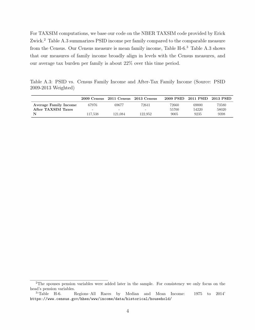
For TAXSIM computations, we base our code on the NBER TAXSIM code provided by Erick

Zwick.2 Table A.3 summarizes PSID income per family compared to the comparable measure

from the Census. Our Census measure is mean family income, Table H-6.3 Table A.3 shows

that our measures of family income broadly align in levels with the Census measures, and

our average tax burden per family is about 22% over this time period.

Table A.3: PSID vs. Census Family Income and After-Tax Family Income (Source: PSID2009-2013 Weighted)

2009 Census 2011 Census 2013 Census 2009 PSID 2011 PSID 2013 PSID

Average Family Income 67976 69677 72641 72660 69000 73580After TAXSIM Taxes - - - 55700 54220 58020N 117,538 121,084 122,952 9005 9235 9398

2The spouses pension variables were added later in the sample. For consistency we only focus on thehead’s pension variables.

3‘Table H-6. Regions–All Races by Median and Mean Income: 1975 to 2014’https://www.census.gov/hhes/www/income/data/historical/household/

4

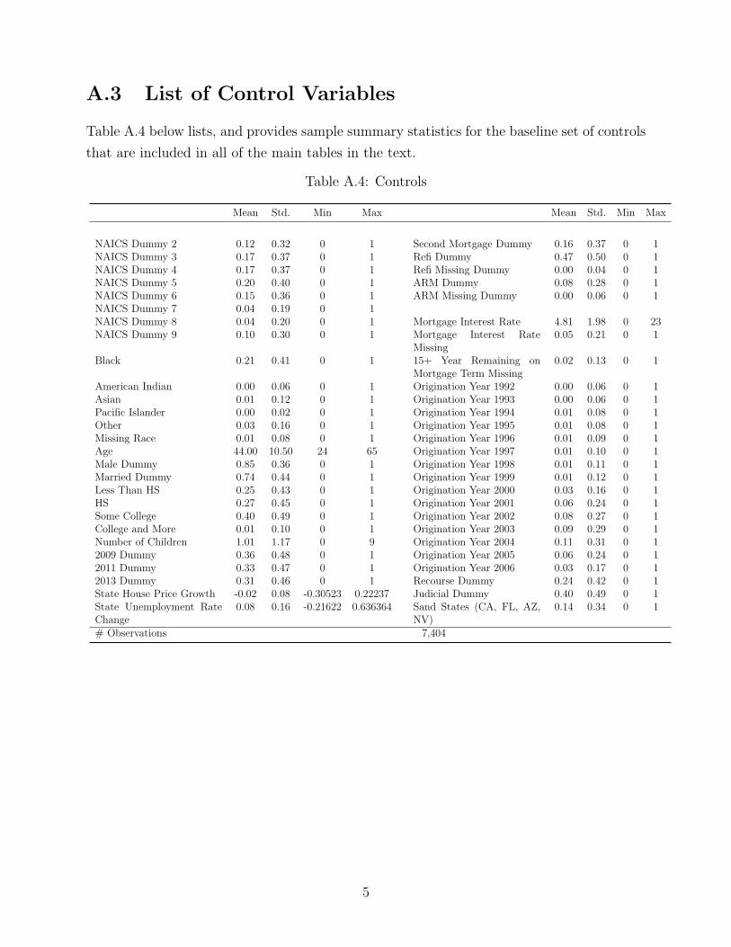
https://www.census.gov/hhes/www/income/data/historical/household/

A.3 List of Control Variables

Table A.4 below lists, and provides sample summary statistics for the baseline set of controls

that are included in all of the main tables in the text.

Table A.4: Controls

Mean Std. Min Max Mean Std. Min Max

NAICS Dummy 2 0.12 0.32 0 1 Second Mortgage Dummy 0.16 0.37 0 1NAICS Dummy 3 0.17 0.37 0 1 Refi Dummy 0.47 0.50 0 1NAICS Dummy 4 0.17 0.37 0 1 Refi Missing Dummy 0.00 0.04 0 1NAICS Dummy 5 0.20 0.40 0 1 ARM Dummy 0.08 0.28 0 1NAICS Dummy 6 0.15 0.36 0 1 ARM Missing Dummy 0.00 0.06 0 1NAICS Dummy 7 0.04 0.19 0 1NAICS Dummy 8 0.04 0.20 0 1 Mortgage Interest Rate 4.81 1.98 0 23NAICS Dummy 9 0.10 0.30 0 1 Mortgage Interest Rate

Missing0.05 0.21 0 1

Black 0.21 0.41 0 1 15+ Year Remaining onMortgage Term Missing

0.02 0.13 0 1

American Indian 0.00 0.06 0 1 Origination Year 1992 0.00 0.06 0 1Asian 0.01 0.12 0 1 Origination Year 1993 0.00 0.06 0 1Pacific Islander 0.00 0.02 0 1 Origination Year 1994 0.01 0.08 0 1Other 0.03 0.16 0 1 Origination Year 1995 0.01 0.08 0 1Missing Race 0.01 0.08 0 1 Origination Year 1996 0.01 0.09 0 1Age 44.00 10.50 24 65 Origination Year 1997 0.01 0.10 0 1Male Dummy 0.85 0.36 0 1 Origination Year 1998 0.01 0.11 0 1Married Dummy 0.74 0.44 0 1 Origination Year 1999 0.01 0.12 0 1Less Than HS 0.25 0.43 0 1 Origination Year 2000 0.03 0.16 0 1HS 0.27 0.45 0 1 Origination Year 2001 0.06 0.24 0 1Some College 0.40 0.49 0 1 Origination Year 2002 0.08 0.27 0 1College and More 0.01 0.10 0 1 Origination Year 2003 0.09 0.29 0 1Number of Children 1.01 1.17 0 9 Origination Year 2004 0.11 0.31 0 12009 Dummy 0.36 0.48 0 1 Origination Year 2005 0.06 0.24 0 12011 Dummy 0.33 0.47 0 1 Origination Year 2006 0.03 0.17 0 12013 Dummy 0.31 0.46 0 1 Recourse Dummy 0.24 0.42 0 1State House Price Growth -0.02 0.08 -0.30523 0.22237 Judicial Dummy 0.40 0.49 0 1State Unemployment RateChange

0.08 0.16 -0.21622 0.636364 Sand States (CA, FL, AZ,NV)

0.14 0.34 0 1

# Observations 7,404

5

A.4 IV Details

In this section we provide details on how the disability and employment instruments are

constructed.

A.4.1 Disability Shocks

We follow the methods of Low and Pistaferri (2015) in identifying a household in which

the head or the spouse has suffered a disability. Specifically, we use information from the

following three PSID survey questions posed to both household heads and spouses: (i) Do

you have any physical or nervous condition that limits the type of work or the amount of work

you can do? If the respondent answers “Yes” the interviewer asks: (ii) Does this condition

keep you from doing some types of work? where the possible answers are: “Yes”, “No”, or

“Can do nothing”. Respondents that answer either “Yes” or “No” are then asked: (iii) For

work you can do, how much does it limit the amount of work you can do? where the possible

answers are given by: “A lot”, “Somewhat”, “Just a little”, or “Not at all”. If the answer to

question (i) is “No” or the answer to question (iii) is “Not at all” then we assume that the

respondent does not have a disability that limits her ability to work. We assume that the

respondent has a severe disability if her response to question (i) is “Yes” and her response

to question (ii) is “Can do nothing” or her response to question (iii) is “A lot”. We assume

that the remainder of respondents have a moderate disability (i.e. they answer “Yes” to

question (i) and either “Somewhat” or “Just a little” to question (iii)).

A.4.2 Bartik Shocks

The Bartik shock is meant to identify exogenous changes in employment status that influence

residual income. The instrument is based on aggregate sectoral employment flows at the

national level and industry shares at the state-level. Specifically, we use data from the

Bureau of Labor Statistics (BLS) to construct the following Bartik state-level employment

shock:

Bartikit =∑

j

shareempl

i,j,t−k ∗∆emplj,t−k,t (1)

where i indexes the state, j indexes the 1-digit NAICs industry code, t indexes the current

survey year (2009, 2011, or 2013), and k indexes the number of years over which the growth

rates are computed. The Bartik shock is constructed by interacting national-level industry

growth in employment, ∆emplj,t−k,t, with the state-level initial composition of employment in

6

industry j, shareempl

i,j,t−k. Calculation of the national-level industry growth rates is performed

using data from all states excluding i. Bartik shocks are used frequently in the labor literature

to instrument for local aggregate demand shocks. The idea behind the Bartik shock is that

employment in all states in all industries is affected by national industry-level employment

movements, but movements in a given industry have a higher impact in a state where the

industry employs a greater share of the population. For example, the Bartik shock calculation

for Florida would place a lower weight on national employment changes in the financial

activities industries than the Bartik shock calculation for New York. In our context, the

Bartik variable is a natural choice for an instrument as state-level, labor demand shocks are

unlikely to be correlated with individual default decisions except through their impact on

the likelihood of job loss and, in turn, income loss. Our measures of employment by industry

and state are taken from the BLS. In particular, we use State and Area Employment, Hours,

and Earnings from the CES.

We construct the Bartik variable over a two-year horizon to maintain consistency with the

biennial frequency of the PSID. (i.e. k = 2). We also estimated specifications using Bartik

shocks constructed over a four-year horizon and found similar results. Finally, we also tried

interacting the Bartik variable with indicator variables corresponding to the industry in

which the household head was employed at the beginning of the horizon. Interacting the

Bartik variable with industry indicators allows the sensitivity of income loss to the exogenous,

state-level, labor demand shocks to differ depending on the particular industry in which the

individual is employed.4. The results from this richer specification proved to be quite similar.

4We included a full set of industry fixed effects among the control variables (not in the instrument set)

7

A.5 Strategic Default with Assets

Table A.5 replicates Table 4 in the main text including information on assets in the PSID.

Household assets, a are computed as the net financial assets of a household: the sum of

checking, saving, money market accounts, government bonds, stocks, and other bonds, less

an imputed 12.73% debt burden on all other unsecured debt obligations. 12.73% is the

average credit card interest rate from 2009-2013 according to the Board of Governors. So in

some cases, ability to pay of households may fall if they have negative net financial assets.

Table A.5: Strategic Default with Assets

Can Pay Can’t Payc < y −m+ a c > y −m+ a > c(V A) y −m+ a < c(V A) Total# share # share # share #(1) (2)=(1)/(7) (3) (4)=(3)/(7) (5) (6)=(5)/(7) (7)

A. AllDefault 95 0.485 40 0.205 61 0.309 196

Population 6184 0.835 570 0.077 655 0.088 7404

Default Rate 0.015 0.071 0.093 0.027B. LTV>90

Default 61 0.525 24 0.210 31 0.265 115Population 1219 0.724 197 0.117 270 0.161 1684

Default Rate 0.050 0.123 0.113 0.069C. LTV<90


Default Rate 0.007 0.043 0.078 0.014

8

A.6 QRM Definitions of Strategic Default

Table A.6 computes default rates among those who meet the QRM definition of affordability,

and those who do not. We use the QRM guidelines to adjust income for taxes, insurance,

alimony, and other debt obligations. If the ratio of combined mortgage payments to adjusted

income is below 43%, the mortgage is deemed affordable. Applying this definition to our

sample, Table A.6 shows that there is a 5x difference in default propensities between those

who meet the QRM definition of affordability (1.6%), and those who don’t (9.2%). Among

those with high LTVs (>90), the default rate among those who do not meet QRM afford-

ability criteria is 17.9% relative to 4.0% for those who do. For those with positive equity,

the level of default drops significantly for both groups.

Table A.6: QRM Based Definitions of Strategic Default

Can Pay Can’t PayDebt to Income<43% Debt to Income>43% Total# share # share #(1) (2)=(1)/(5) (3) (4)=(3)/(5) (5)

A. AllDefault 100 0.508 97 0.492 196Population 6359 0.859 1045 0.141 7404

Default Rate 0.016 0.092 0.027B. LTV>90

Default 54 0.465 62 0.535 115Population 1338 0.794 346 0.206 1684

Default Rate 0.040 0.179 0.069C. LTV<90

Default 46 0.571 35 0.429 81Population 5021 0.878 699 0.122 5720

Default Rate 0.009 0.050 0.014

9

A.7 Baseline Regressions with DTI

Table A.7 reproduces Table 5 in the main text using the logarithm of the debt-to-income

ratio, or DTI, (i.e. log(my)) as the main independent regressor instead of the logarithm of

residual income. Columns (1)–(3) report OLS coefficients, and columns (4)–(6) report logit

coefficients with average marginal effects in square parentheses. As in Table 5, the interaction

term is computed at the interquartile range for the logit specification. The coefficients can

be interpreted as semi-elasticities. For example, the point estimate in column (1) implies

that a 10% increase in DTI is associated with a 0.39 percentage point higher default rate.

Table A.7: Debt to Income Ratio Results: Linear Probability Model Cols (1) to (3), LogitCoefficients Cols (4) to (6) (with AME in square brackets, interaction at interquartile rangeof residual income), Dependent Variable is 60+ Days Late Indicator.

(1) (2) (3) (4) (5) (6)

Loan to Value Ratio 0.058*** 0.071*** 0.259*** 1.568*** 1.548*** 2.341***(6.09) (6.06) (7.17) (8.51) (7.56) (4.57)

[0.047***] [0.045***] [0.043***]Log of DTI 0.039*** 0.030*** -0.034*** 1.406*** 1.110*** 0.630**

(8.47) (6.64) (-3.48) (10.93) (7.61) (2.02)[0.043***] [0.032***] [0.033***]

Log of DTI * LTV 0.103*** 0.563*(6.39) (1.71)

[0.029***]Constant 0.066*** -0.019 -0.134*** -2.318*** -4.024*** -4.630***

(5.30) (-0.69) (-3.88) (-8.45) (-3.28) (-3.61)

Observations 7,402 7,402 7,402 7,402 7,402 7,402R-squared 0.036 0.077 0.093 - - -Demographic Controls? N Y Y N Y YMortgage Controls? N Y Y N Y YState Controls? N Y Y N Y Y

10

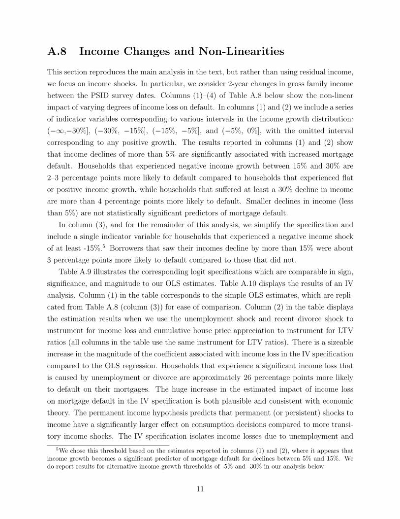
A.8 Income Changes and Non-Linearities

This section reproduces the main analysis in the text, but rather than using residual income,

we focus on income shocks. In particular, we consider 2-year changes in gross family income

between the PSID survey dates. Columns (1)–(4) of Table A.8 below show the non-linear

impact of varying degrees of income loss on default. In columns (1) and (2) we include a series

of indicator variables corresponding to various intervals in the income growth distribution:

(−∞,−30%], (−30%, −15%], (−15%, −5%], and (−5%, 0%], with the omitted interval

corresponding to any positive growth. The results reported in columns (1) and (2) show

that income declines of more than 5% are significantly associated with increased mortgage

default. Households that experienced negative income growth between 15% and 30% are

2–3 percentage points more likely to default compared to households that experienced flat

or positive income growth, while households that suffered at least a 30% decline in income

are more than 4 percentage points more likely to default. Smaller declines in income (less

than 5%) are not statistically significant predictors of mortgage default.

In column (3), and for the remainder of this analysis, we simplify the specification and

include a single indicator variable for households that experienced a negative income shock

of at least -15%.5 Borrowers that saw their incomes decline by more than 15% were about

3 percentage points more likely to default compared to those that did not.

Table A.9 illustrates the corresponding logit specifications which are comparable in sign,

significance, and magnitude to our OLS estimates. Table A.10 displays the results of an IV

analysis. Column (1) in the table corresponds to the simple OLS estimates, which are repli-

cated from Table A.8 (column (3)) for ease of comparison. Column (2) in the table displays

the estimation results when we use the unemployment shock and recent divorce shock to

instrument for income loss and cumulative house price appreciation to instrument for LTV

ratios (all columns in the table use the same instrument for LTV ratios). There is a sizeable

increase in the magnitude of the coefficient associated with income loss in the IV specification

compared to the OLS regression. Households that experience a significant income loss that

is caused by unemployment or divorce are approximately 26 percentage points more likely

to default on their mortgages. The huge increase in the estimated impact of income loss

on mortgage default in the IV specification is both plausible and consistent with economic

theory. The permanent income hypothesis predicts that permanent (or persistent) shocks to

income have a significantly larger effect on consumption decisions compared to more transi-

tory income shocks. The IV specification isolates income losses due to unemployment and

5We chose this threshold based on the estimates reported in columns (1) and (2), where it appears thatincome growth becomes a significant predictor of mortgage default for declines between 5% and 15%. Wedo report results for alternative income growth thresholds of -5% and -30% in our analysis below.

11

divorce shocks, which are both significant life events and thus, are likely to have persistent

effects. In other words, the IV specification is isolating more permanent income shocks,

which theory predicts should lead to a much larger impact on the propensity to default.

Column (3) shows the reduced form of Column (2) where the default indicator is directly

regressed on job loss and divorce indicators. In Column (4) of Table A.10 we modify the

instrument set by substituting for the unemployment variables with indicators of involuntary

unemployment spells only (for both the head and spouse). In addition, we include a set of

indicator variables corresponding to the number of prior unemployment spells as additional

controls. The income loss coefficient decreases slightly (from 0.26 to 0.20), but is still very

large in magnitude and statistically significant (at the 5 percent level). An income loss of

at least 15% (between surveys) caused by an involuntary unemployment spell or divorce is

estimated to increase the likelihood of default by 20 percentage points. Column (5) displays

the reduced form regression results, where the default indicator is regressed directly on the

involuntary unemployment shocks. The estimates are of comparable magnitudes with those

in column (3).

Column (6) in Table A.10 displays the results when we instrument for income loss using

the disability shock and the Bartik employment shocks. We construct the Bartik variable

over a two-year horizon (i.e. k = 2)6 to maintain consistency with the biennial frequency

of the PSID and our other results. We interact the Bartik variable with indicator variables

corresponding to the industry in which the household head was employed at the beginning

of the horizon.7 In column (6) of Table A.10, the coefficient estimate is 0.26 (statistically

significant at the 5% level), which is very similar in magnitude to the estimates we obtained

using unemployment spells and recent divorces as instruments (columns (2) and (4)). The

first stage results displayed in Table A.11, (column (6) in Panel B) show that the disability

indicator is a strong predictor of severe income loss, which is consistent with the findings in

Low and Pistaferri (2015). For space considerations we report the first stage estimates for

the Bartik variables in the Appendix instead of Table A.11.8 The reduced form specification

results reported in column (7) of Table A.10 show that the disability variable has a slightly

6We also estimated specifications using Bartik shocks constructed over a four-year horizon and foundsimilar results.

7Interacting the Bartik variable with industry indicators allows the sensitivity of income loss to theexogenous, state-level, labor demand shocks to differ depending on the particular industry in which theindividual is employed. We include a full set of industry fixed effects among the control variables (not in theinstrument set).

8Virtually all of the Bartik coefficients have the expected negative sign, so that positive state-level, labordemand shocks (i.e. increases in employment) are associated with a lower likelihood of significant income loss,however, they are not statistically significant, which suggests that they are not especially strong instrumentsfor income loss at the household-level. However, it is clear from the weak instrument test p-values reported inTable A.10 that the combination of the disability and Bartik variables constitute a strong set of instruments.

12

smaller direct impact on mortgage default compared to the the unemployment and divorce

variables.

In column (8) of Table A.10 we substitute the severe disability shock into the instrument

set. Households that experience severe disability shocks are more likely to suffer more per-

sistent income losses compared to households that suffer more moderate disability shocks,

and thus we would expect the effect of income loss on default to increase as a result of this

substitution. This is exactly what we find as the point estimate of the effect of income loss on

mortgage default increases from 0.26 to 0.32.9 In addition, the first stage results show that

households that experience a severe disability shock are about twice as likely to experience

an income loss of at least 15%, and the reduced form estimates (column (9)) show that they

are also much more likely to default on their mortgage debt.

9The difference between the two point estimates is not statistically significant however.

13

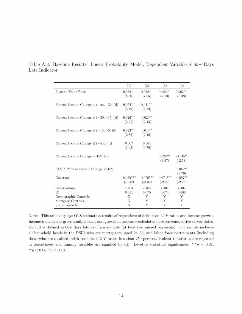
Table A.8: Baseline Results: Linear Probability Model, Dependent Variable is 60+ DaysLate Indicator.

(1) (2) (3) (4)

Loan to Value Ratio 0.082∗∗∗ 0.082∗∗∗ 0.083∗∗∗ 0.062∗∗∗

(8.60) (7.06) (7.10) (5.38)

Percent Income Change ∈ (−∞,−30] (d) 0.054∗∗∗ 0.041∗∗∗

(5.49) (4.39)

Percent Income Change ∈ (−30,−15] (d) 0.026∗∗∗ 0.020∗∗

(3.21) (2.45)

Percent Income Change ∈ (−15,−5] (d) 0.022∗∗∗ 0.019∗∗

(2.82) (2.46)

Percent Income Change ∈ (−5, 0] (d) 0.007 0.004(1.03) (0.70)

Percent Income Change <-15% (d) 0.029∗∗∗ -0.045∗∗

(4.47) (-2.58)

LTV * Percent Income Change <-15% 0.105∗∗∗

(3.79)Constant -0.035*** -0.076*** -0.074*** -0.057**

(-5.42) (-3.02) (-2.92) (-2.28)

Observations 7,404 7,404 7,404 7,404R2 0.031 0.075 0.074 0.080Demographic Controls N Y Y YMortgage Controls N Y Y YState Controls N Y Y Y

Notes: This table displays OLS estimation results of regressions of default on LTV ratios and income growth.

Income is defined as gross family income and growth in income is calculated between consecutive survey dates.

Default is defined as 60+ days late as of survey date (at least two missed payments). The sample includes

all household heads in the PSID who are mortgagors, aged 24–65, and labor force participants (including

those who are disabled) with combined LTV ratios less than 250 percent. Robust t-statistics are reported

in parentheses and dummy variables are signified by (d). Level of statistical significance: ∗∗∗p < 0.01,∗∗p < 0.05, ∗p < 0.10.

14

Table A.9: Baseline Results: Logit, Dependent Variable is 60+ Days Late Indicator. AverageMarginal Effects Reported.

(1) (2) (3) (4)

Percent Income Change ∈ (−∞,−30] (d) 0.063*** 0.042***(5.15) (4.38)

Percent Income Change ∈ (−30,−15] (d) 0.032*** 0.020**(3.05) (2.37)

Percent Income Change ∈ (−15,−5] (d) 0.028*** 0.025***(2.71) (2.61)

Percent Income Change ∈ (−5, 0] (d) 0.007 0.006(0.79) (0.66)

Loan to Value Ratio 0.062*** 0.049*** 0.050*** 0.050***(10.38) (8.33) (8.36) (8.34)

Percent Income Change <-15% (d) 0.025*** 0.025***(4.40) (4.42)

LTV * % Income Ch. <-15% (d) 0.051***(3.48)

Observations 7,404 7,404 7,404 7,404Demographic Controls N Y Y YMortgage Controls N Y Y YState Controls N Y Y Y

Notes: This table displays average marginal effects from logit regressions of default on LTV ratios and income

growth. Income is defined as gross family income and growth in income is calculated between consecutive

survey dates. Default is defined as 60+ days late as of survey date (at least two missed payments). The

sample includes all household heads in the PSID who are mortgagors, aged 24–65, and labor force participants

(including those who are disabled) with combined LTV ratios less than 250 percent. Robust t-statistics

are reported in parentheses and dummy variables are signified by (d). Level of statistical significance:∗∗∗p < 0.01, ∗∗p < 0.05, ∗p < 0.10.

15

Table A.10: IV Results: Dependent Variable is 60+ DL Indicator, 1st Endogenous Variable is 2-Year Income Change, 2ndEndogenous Variable is LTV. Col (1) is OLS, Cols (2) and (3) use unemployment and divorce as IVs for income. Cols (4) and(5) use invol. unemployment and divorce. Cols (6) and (7) use disability and Bartik shocks, and Cols (8) and (9) use severedisability and Bartik shocks. Cumulative HP growth is IV for LTV in all Columns.

Dependent Variable: 60+ Days Delinquent

(1) (2) (3) (4) (5) (6) (7) (8) (9)

LTV Ratio 0.083*** 0.167*** 0.147*** 0.175*** 0.146*** 0.172*** 0.150*** 0.178*** 0.149***(7.10) (3.15) (3.06) (3.46) (3.04) (3.35) (3.14) (3.35) (3.13)

Percent Income Change <-15% (d) 0.029*** 0.264*** 0.199** 0.233** 0.266**(4.47) (4.26) (2.45) (2.27) (2.13)

Unemployed Head Last Year (d) 0.053***(4.12)

Unemployed Spouse Last Year (d) 0.031**(2.36)

Recent Divorce (d) 0.034 0.034(1.40) (1.43)

Involuntary Layoff (d) 0.035**(2.04)

Involuntary Layoff, Spouse (d) 0.054*(1.88)

Disability Shock (d) 0.018*(1.80)

Severe Disability Shock (d) 0.051*(1.75)

IV for LTV Ratio: . HPA Since HPA Since HPA Since HPA Since HPA Since HPA Since HPA Since HPA Since. Purchase Purchase Purchase Purchase Purchase Purchase Purchase Purchase

IV for Income: . Job Loss, Invol. Job Loss, Disability, Severe Disability,. Recent Divorce Recent Divorce Bartik Shock Bartik Shock

Observations 7,404 7,404 7,404 7,404 7,404 7,404 7,404 7,404 7,404R2 0.074 . 0.069 . 0.067 . 0.061 . 0.062Demographic Controls Y Y Y Y Y Y Y Y YMortgage Controls Y Y Y Y Y Y Y Y YState Controls Y Y Y Y Y Y Y Y YControl for Prior Unempl Spells N N N Y Y N N N N

IV Diagnostics

Over ID Pval, Null Valid . 0.271 . 0.237 . 0.916 . 0.923 .Weak ID Pval, Null Weak . 0 0 3.49e-10 0 0.00252 0 0.00317 0

Notes: This table displays a set of estimation from regressions of default on LTV ratios and income loss. Default is defined as 60+ days late as of

survey date (at least two missed payments). Income loss is defined as a drop in household income of at least 15% from the previous interview. The

sample includes all household heads in the PSID who are mortgagors, aged 24–65, and labor force participants (including those who are disabled)

with combined LTV ratios less than 250 percent in 2009, 2011, and 2013. Robust t-statistics are reported in parentheses and dummy variables are

signified by (d). Level of statistical significance: ∗∗∗p < 0.01, ∗∗p < 0.05, ∗p < 0.10.

16

A.9 Robustness

Table A.12 below displays robustness results for our main specifications in Table 7 in the

text. Columns (1) and (2) include state fixed effects. These specifications yield consistent,

although somewhat stronger, parameter estimates when compared to columns (4) and (6),

respectively, of Table 7. Columns (3) and (4) of Table A.12 use Bartik shocks that are

constructed with 4 year and 1 year CES employment changes by state and industry, respec-

tively. Our estimates are very close to Columns (6) and (8) in Table 7. Columns (5) and

(6) include a dummy for negative equity instead of a continuous variable, and for low LTVs,

the dummy on negative equity implies a stronger effect of house price changes on default.

An LTV of 1 in column (1) is associated with a 28% likelihood of default versus a 34%

likelihood of default in column (5). On the other hand, for higher LTVs, the relationship is

reversed: an LTV of 1.2 in column (1) is associated with a 33% likelihood of default versus a

34% likelihood of default in column (5). Columns (7) and (8) combine the head and spouse

disability shocks to obtain more power, and again, we see similar results to the main table

in the text. Additionally, in every case, the model passes over-identification tests at the 1%,

5%, and 10% statistical levels.

Table A.13 displays the first stages of the various regressions in Table A.12, where each

specification has two first stages corresponding to LTV and residual income. Panel A shows

that cumulative house price growth is a strong instrument for LTV, and Panel B shows

that the alternate instruments for income yield strong first stage results. In every case, the

alternate sets of instruments pass weak identification tests.

17

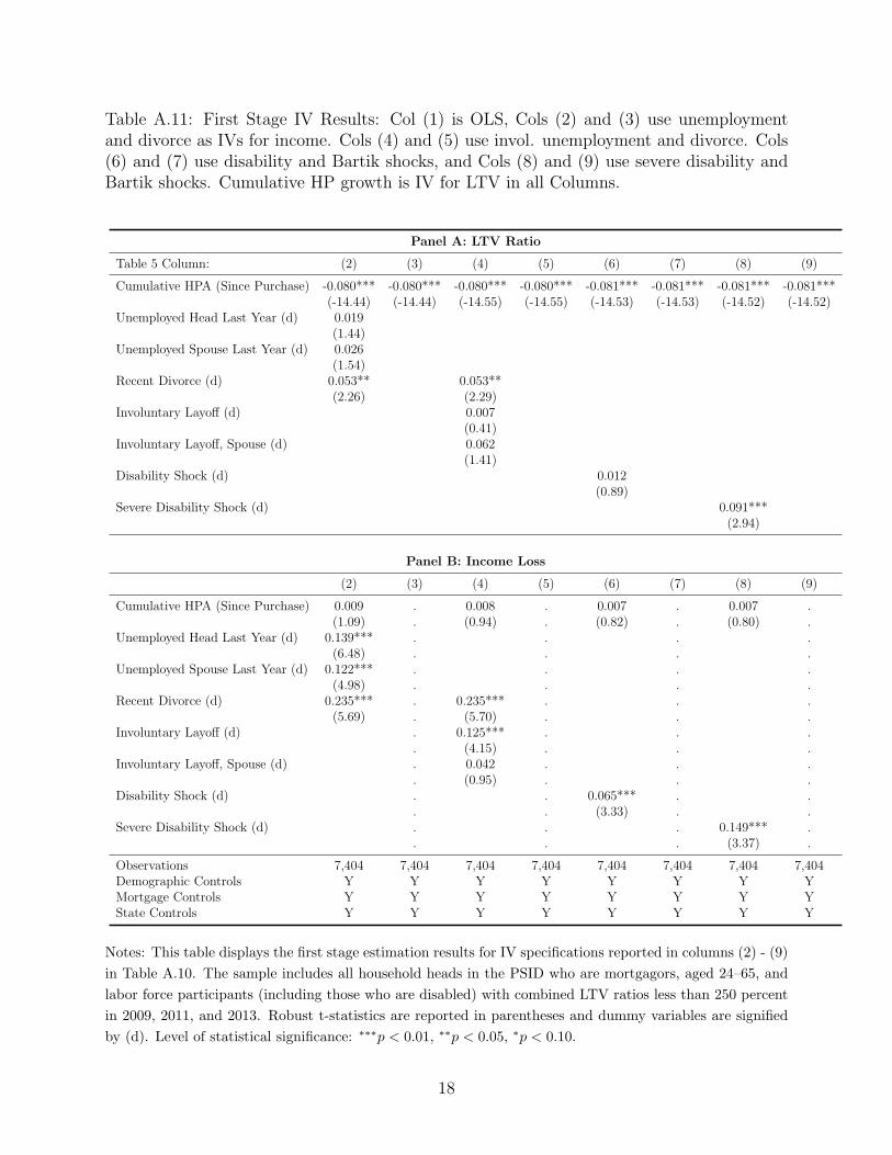
Table A.11: First Stage IV Results: Col (1) is OLS, Cols (2) and (3) use unemploymentand divorce as IVs for income. Cols (4) and (5) use invol. unemployment and divorce. Cols(6) and (7) use disability and Bartik shocks, and Cols (8) and (9) use severe disability andBartik shocks. Cumulative HP growth is IV for LTV in all Columns.

Panel A: LTV Ratio

Table 5 Column: (2) (3) (4) (5) (6) (7) (8) (9)

Cumulative HPA (Since Purchase) -0.080*** -0.080*** -0.080*** -0.080*** -0.081*** -0.081*** -0.081*** -0.081***(-14.44) (-14.44) (-14.55) (-14.55) (-14.53) (-14.53) (-14.52) (-14.52)

Unemployed Head Last Year (d) 0.019(1.44)

Unemployed Spouse Last Year (d) 0.026(1.54)

Recent Divorce (d) 0.053** 0.053**(2.26) (2.29)

Involuntary Layoff (d) 0.007(0.41)

Involuntary Layoff, Spouse (d) 0.062(1.41)

Disability Shock (d) 0.012(0.89)

Severe Disability Shock (d) 0.091***(2.94)

Panel B: Income Loss

(2) (3) (4) (5) (6) (7) (8) (9)

Cumulative HPA (Since Purchase) 0.009 . 0.008 . 0.007 . 0.007 .(1.09) . (0.94) . (0.82) . (0.80) .

Unemployed Head Last Year (d) 0.139*** . . . .(6.48) . . . .

Unemployed Spouse Last Year (d) 0.122*** . . . .(4.98) . . . .

Recent Divorce (d) 0.235*** . 0.235*** . . .(5.69) . (5.70) . . .

Involuntary Layoff (d) . 0.125*** . . .. (4.15) . . .

Involuntary Layoff, Spouse (d) . 0.042 . . .. (0.95) . . .

Disability Shock (d) . . 0.065*** . .. . (3.33) . .

Severe Disability Shock (d) . . . 0.149*** .. . . (3.37) .

Observations 7,404 7,404 7,404 7,404 7,404 7,404 7,404 7,404Demographic Controls Y Y Y Y Y Y Y YMortgage Controls Y Y Y Y Y Y Y YState Controls Y Y Y Y Y Y Y Y

Notes: This table displays the first stage estimation results for IV specifications reported in columns (2) - (9)

in Table A.10. The sample includes all household heads in the PSID who are mortgagors, aged 24–65, and

labor force participants (including those who are disabled) with combined LTV ratios less than 250 percent

in 2009, 2011, and 2013. Robust t-statistics are reported in parentheses and dummy variables are signified

by (d). Level of statistical significance: ∗∗∗p < 0.01, ∗∗p < 0.05, ∗p < 0.10.

18

Table A.12: Robustness Results for Table 7.

(1) (2) (3) (4) (5) (6) (7) (8)

Loan to Value Ratio 0.287*** 0.255*** 0.184*** 0.190*** 0.181*** 0.194***(3.65) (3.67) (3.64) (3.62) (3.60) (3.77)

Log Residual Income -0.242** -0.178* -0.099* -0.124* -0.289** -0.098* -0.094* -0.116*(-2.30) (-1.94) (-1.91) (-1.95) (-2.53) (-1.76) (-1.85) (-1.96)

LTV>100 (d) 0.346*** 0.297***(2.93) (3.30)

IV for LTV: HPA Since HPA Since HPA Since HPA Since HPA Since HPA Since HPA Since HPA SincePurchase Purchase Purchase Purchase Purchase Purchase Purchase Purchase

IV for Income: Invol. Job Loss, Disability, Disability, Disability, Invol. Job Loss, Disability, Combined Disability, Combined Severe Disability,Head & Spouse Bartik Shock Bartik Shock (4yr) Bartik Shock (1yr) Head & Spouse Bartik Shock Bartik Shock Bartik Shock

Observations 7,404 7,404 7,404 7,404 7,339 7,339 7,404 7,404Demographic Controls? Y Y Y Y Y Y Y YMortgage Controls? Y Y Y Y Y Y Y YState Controls? Y Y Y Y Y Y Y YState FEs? Y Y N N N N N NJob Loss FEs? Y N N N Y N N NJtest Pval Null Valid 0.305 0.329 0.155 0.214 0.313 0.107 0.420 0.333Weak ID Pval Null Weak 0.000225 0.00415 1.22e-07 1.83e-05 0.000425 6.81e-07 4.66e-08 2.90e-08

Notes: See Table 7 for additional notes. Col. 1 and Col. 2 include state FEs. Col. 3 and Col. 4 construct Bartik shocks using 4 year and 1 year

employment changes by state and industry, respectively. Col. 5 and Col. 6 use a dummy for negative equity instead of a continuous variable. Col. 7

and Col. 8 combined the head and spouse disability shocks. Level of statistical significance: ∗∗∗p < 0.01, ∗∗p < 0.05, ∗p < 0.10.

19

Table A.13: First Stages of the Robustness Results for Table 7.

A. LTV First Stage (1) (2) (3) (4) (5) (6) (7) (8)

Cumulative State HP Growth from Purchase Date -0.076*** -0.076*** -0.081*** -0.081*** -0.081*** -0.081*** -0.081*** -0.081***(-13.59) (-13.42) (-14.46) (-14.53) (-14.53) (-14.53) (-14.53) (-14.52)

Bartik Instrument (2 Yr. Ch.) 0.933 0.424 0.470(0.74) (0.50) (0.55)

Transition into Disability, Head (d) 0.004 0.003 0.003 0.003(0.20) (0.16) (0.16) (0.16)

Transition into Disability, Spouse (d) 0.012 0.014 0.014 0.014(0.65) (0.80) (0.80) (0.80)

Involuntary Unemployment, Head (d) 0.025(1.21)

Involuntary Unemployment, Spouse (d) 0.000(0.00)

Bartik Instrument (4 Yr. Ch.) -0.070(-0.14)

Bartik Instrument (1 Yr. Ch.) 0.164(0.11)

Transition into Disability Head or Spouse (d) 0.012(0.89)

Transition into Severe Disability Head or Spouse (d) 0.091***(2.96)

Observations 7,404 7,404 7,404 7,404 7,404 7,404 7,404 7,404R-squared 0.372 0.370 0.351 0.351 0.351 0.351 0.351 0.352Demographic Controls? Y Y Y Y Y Y Y YMortgage Controls? Y Y Y Y Y Y Y YState Controls? Y Y Y Y Y Y Y YState FEs? Y Y N N N N N NJob Loss FEs? Y N N N Y N N N

B. Income First Stage (1) (2) (3) (4) (5) (6) (7) (8)

Cumulative State HP Growth from Purchase Date -0.035*** -0.034** -0.026* -0.023* -0.019 -0.022 -0.025* -0.024*(-2.65) (-2.53) (-1.92) (-1.71) (-1.46) (-1.61) (-1.83) (-1.81)

Bartik Instrument (2 Yr. Ch.) 5.605* 10.463*** 10.328*** 10.092***(1.66) (4.64) (4.61) (4.49)

Transition into Disability, Head (d) -0.134*** -0.145*** -0.146*** -0.151***(-2.58) (-2.78) (-2.81) (-2.88)

Transition into Disability, Spouse (d) -0.087** -0.092** -0.091** -0.084**(-2.06) (-2.17) (-2.15) (-2.01)

Involuntary Unemployment, Head (d) -0.198*** -0.217***(-3.85) (-4.16)

Involuntary Unemployment, Spouse (d) 0.094 0.081(1.54) (1.29)

Bartik Instrument (4 Yr. Ch.) 6.240***(4.85)

Bartik Instrument (1 Yr. Ch.) 14.649***(3.66)

Transition into Disability Head or Spouse (d) -0.126***(-3.69)

Transition into Severe Disability Head or Spouse (d) -0.281***(-3.83)

Observations 7,404 7,404 7,404 7,404 7,339 7,339 7,404 7,404R-squared 0.347 0.339 0.321 0.320 0.325 0.319 0.321 0.321Demographic Controls? Y Y Y Y Y Y Y YMortgage Controls? Y Y Y Y Y Y Y YState Controls? Y Y Y Y Y Y Y YState FEs? Y Y N N N N N NJob Loss FEs? Y N N N Y N N N

Notes: See Table 7 and Table A.12 for additional notes.

20

A.10 Comparison of Default Rates in PSID and Mc-

Dash/Equifax

Table A.14 expands the comparison of default rates and LTV ratio distributions between

the PSID and McDash/Equifax (CRISM) datasets performed in Section 2.2 of the paper.

Specifically, it includes results for 2011 and 2013 along with 2009.

For both PSID and CRISM, we break out the LTV ratio distribution into three intervals,

LTV ≤ 80, 80 < LTV < 100, and LTV ≥ 100, and show the fraction of the sample in each

interval and the default rate within each interval. We calculate LTV shares and default rates

for three different CRISM samples. The first sample includes all active first lien mortgages,

and is most comparable to aggregate default rates commonly reported by the Mortgage

Bankers Association and McDash.10 The second sample includes only first liens associated

with owner-occupant properties. The PSID only asks respondents for information on the

loans associated with their principal residence, so this sample of mortgages should be more

comparable to the PSID sample. Finally, the third sample also includes only first lien,

owner-occupants, but also eliminates mortgages that are reported by the servicer as being in

the foreclosure process where the borrower appears to have vacated the property and moved

elsewhere.11 This additional restriction brings the CRISM sample closer to the PSID sample

for comparison purposes because, again, the PSID only asks questions about mortgages

associated with the respondents’ current, principal residence. For example, a respondent

who has moved out of a property that is still in the foreclosure process and is now renting,

would be considered to be a renter in the PSID, and no information on the delinquent

mortgage would be collected.

Focusing on the 2009 statistics in the top panel of the table, the overall default rate in

the PSID is 3.9% while the default rate in the broadest CRISM sample is 8.6%. This is

a large discrepancy and on its face calls into question the representativeness of the PSID

sample on the dimension of mortgage performance. However, when we throw investors

and second homes out of the CRISM sample the aggregate default rate falls from 8.6% to

6.5%. Eliminating mortgages in foreclosure for which the borrower is no longer living in the

property further reduces the CRISM default rate to 5.4%. We see a very similar pattern

for 2011 and 2013. Thus, adjusting the CRISM sample to more closely align with the PSID

sample reduces the default rate discrepancy from 4–5 percentage points to 1.0–1.5 percentage

points.

10Including second liens in the sample has almost no impact on the default rate, so for space considerationswe decided to begin with a sample of only first liens.

11The CRISM data provide the zip codes of each mortgage borrower’s mailing address and the propertyaddress. When the two zip codes differ, we assume that the borrower no longer resides in the property.

21

In addition to the sample differences, Table A.14 shows that there are material differences

between the LTV distributions in the PSID and CRISM. For example, in both 2009 and 2011,

the fraction of high LTV mortgages (≥ 100) is about 10 percentage points higher in CRISM

compared to the PSID. The default rates associated with high LTV mortgages are similarly

high in both datasets, which suggests that the composition of high LTV mortgages is similar

across the two datasets.12 Since the default rates associated with high LTV mortgages are

much higher than those associated with lower LTV loans, the smaller share of high LTV

loans in the PSID sample has a negative effect on the overall default rate and drives some of

the discrepancy in the aggregate default rates between the two datasets. To see this, in the

last column of the table, we recalculate the default rate in the PSID using LTV shares from

CRISM (the shares that correspond to Sample (3)). In both 2009 and 2011 this adjustment

almost completely closes the remaining gap between default rates,13 increasing the PSID

default rate to virtually the same level as the CRISM default rate (5.4% in 2009 and 4.8%

in 2011).

12This is notable because the LTV ratios are calculated in very different ways. In the PSID, we calculateLTV ratios using the self-reported remaining mortgage balance and the self-reported house value at the timeof the survey. In contrast, the LTV ratio in CRISM is based on the actual remaining mortgage balancereported by the servicer and an estimate of the value of the house based on the cumulative change in thezip code-level house price index since the month in which the mortgage was originated. The fact that thedefault rates within each LTV interval are quite similar across both datasets suggests that composition ofloans in each interval is similar.

13In 2013, the adjustment does not make a material difference because the LTV shares are very similar inboth datasets.

22

Table A.14: Comparison of Default Rates in the PSID and McDash/Equifax

2009

LTV Category

McDash/Equifax PSID

Sample (1): Sample (2): Sample (3):First Liens Only First Liens Only First Liens Only

No Investors No Investors, Living in Home Default Rate using

Share Default Rate Share Default Rate Share Default Rate Share Default Rate CRISM Shares

LTV ≥ 100 21.8% 23.1% 21.0% 17.4% 20.7% 14.0% 10.5% 16.0%80 < LTV < 100 24.2% 8.4% 24.1% 6.6% 24.2% 5.7% 18.8% 3.8%LTV ≤ 80 54.0% 2.8% 55.0% 2.2% 55.1% 2.0% 70.7% 2.2%

All 8.6% 6.5% 5.4% 3.9% 5.4%

2011

LTV Category

McDash/Equifax PSID




LTV ≥ 100 23.4% 22.0% 22.4% 14.3% 22.2% 12.4% 12.7% 12.6%80 < LTV < 100 26.3% 7.6% 27.1% 5.1% 27.5% 4.6% 22.1% 3.8%LTV ≤ 80 50.2% 3.1% 50.4% 2.1% 50.3% 1.9% 65.2% 2.0%

All 8.7% 5.7% 5.0% 3.8% 4.8%

2013

LTV Category

McDash/Equifax PSID




LTV ≥ 100 10.4% 24.2% 9.4% 17.8% 9.0% 16.0% 10.1% 12.6%80 < LTV < 100 24.2% 8.4% 26.6% 6.1% 26.5% 5.4% 24.2% 4.9%LTV ≤ 80 64.4% 3.3% 64.1% 2.4% 64.5% 2.2% 65.7% 1.1%

All 6.7% 4.8% 4.3% 3.2% 3.1%

Notes: This table compares mortgage default rates and LTV distributions in the PSID and McDash/Equifax (CRISM) datasets. CRISM is a

proprietary dataset that contains credit bureau data on individual consumers’ credit histories matched to LPS mortgage servicing data.

23

A.11 Strategic Default Estimates using PSID-McDash/Equifax

Weights

To further address concerns regarding representativeness of the PSID, we generate a set of

weights using McDash/Equifax (CRISM) data, which we have made available to the pub-

lic.14 We do so using post-stratification. We split the restricted PSID sample (i.e. prime

age, LTV<2.5, single-family, owner-occupied, 2009-2013) into a set of 225 bins. We impose

the same mortgage criteria on CRISM and split it into the same 225 bins. We then compute

ratios of population shares in those bins. This allows us to produce an identical distribution

of individuals across bins between CRISM and the PSID. For whites, we use 5 LTV bins

{ LTV<.8, .8<LTV<.9, .9<LTV<1, 1<LTV<1.1, 1.1<LTV<2.5 }, 5 Age bins { 24-34,35-

40,41-47,48-55,56-65} (which correspond to age quintiles), and 5 Principal Remaining Bins

{Less than 59k, 59k-100k,101k-148k,149k-216k,216k and more} (which correspond to prin-

cipal remaining quintiles). For non-whites, we collapse non-populated cells, which primarily

include minorities with severe negative equity. We use 4 LTV bins { LTV<.8, .8<LTV<.9,

.9<LTV<1, 1<LTV<2.5 }, 5 Age bins (same as above), and 5 Principal Remaining Bins

(same as above). Of the 225 possible bins for whites, all bins are populated. Of the 225 bins

for non-whites, 223 are populated. Therefore our weights allow us to almost exactly match

the 4-way joint distribution of age, LTV, principal, and race in CRISM.

Table A.15 summarizes the LTV distribution of the PSID under 3 sets of weights: CRISM

weights (Column (2)), raw PSID (Column (3)), family weights applied to the PSID (Column

(4)). By construction, the CRISM weights match the LTV distribution. We also match

the LTV distribution when we split by principal remaining, age, and race (subject to the

collapsed LTV bins for non-whites).

Table A.16 reproduces our main strategic default table using the CRISM shares. In

general, there are economically insignificant differences between the two tables. We find

that the share of strategic defaulters drops from 37.7% in Table A.1 to 37.2% in Table A.16.

Given that the two sets of results are so similar, there are strong reasons to use the PSID

family weights, rather than the CRISM weights, since the PSID weights use many more

post-stratum.

In our baseline OLS regressions, Table A.17, we see nearly identical point estimates to

the unweighted OLS regressions. The coefficient on LTV is 0.078 in Table 5 Column (2)

for the unweighted regressions, and the coefficient on LTV in Table A.17 Column (2) is

.085 for the weighted regression. The coefficient on log residual income is -0.025 in Table

14The data and the code to build the weights are available here:(https://sites.google.com/site/kyleherkenhoff/research)

24

https://sites.google.com/site/kyleherkenhoff/research

Table A.15: Weighted LTV Distribution, CRISM vs PSID (Years: Pooled 2009-2013)

CRISM Shares under PSIDSample Restrictions for Re-gressions

PSID Shares under PSIDSample Restrictions for Re-gressions using CRISMWeights

PSID Shares under PSIDSample Restrictions for Re-gressions, Raw

PSID Shares under PSIDSample Restrictions forRegressions using PSIDFamily Weights

(1) (2) (3) (4)

LTV<.8 51.0 51.0 59.4 63.5.8<LTV<.9 16.6 16.6 14.8 13.8.9<LTV<1 15.3 15.3 15.1 13.11<LTV<1.1 10.3 10.3 6.3 4.81.1<LTV<2.5 6.9 6.9 4.5 4.9

Notes: CRISM and PSID restricted samples (i.e. prime age, LTV<2.5, single-family, owner-occupied,

2009-2013).

Table A.16: Strategic Default, Weighted Using PSID-McDash/Equifax Weights


A. AllDefault 87 0.372 90 0.386 57 0.245 234

Population 5147 0.695 1791 0.242 469 0.063 7404





Default Rate 0.007 0.025 0.060 0.014

Notes: Weighted using PSID-CRISM weights described in the text. CRISM and PSID restricted samples

(i.e. prime age, LTV<2.5, single-family, owner-occupied, 2009-2013).

25

5 Column (1) for the unweighted regressions, and the coefficient on log residual income in

Table A.17 Column (2) is -.026 for the weighted regression. The weights do little to the

point estimates since the post-stratum are controls. In general, if the sample is random and

the post-stratum are controls, i.e. the weighting criteria are being “conditioned-on,” then

the weights are redundant and merely introduce noise.

Table A.17: Baseline Results: Linear Probability Model Cols (1) to (3), Logit CoefficientsCols (4) to (6) (with AME in square brackets, interaction at interquartile range of residualincome), Dependent Variable is 60+ Days Late Indicator.

(1) (2) (3) (4) (5) (6)

Loan to Value Ratio 0.084*** 0.085*** 1.042*** 2.141*** 2.213*** 1.574(7.13) (5.67) (4.80) (10.97) (9.73) (0.65)

[0.059***] [0.059***] [0.059***]Log Residual Income -0.036*** -0.026*** 0.039*** -0.919*** -0.814*** -0.874***

(-6.85) (-4.73) (3.18) (-10.92) (-8.14) (-4.17)[-0.025***] [-0.022***] [-0.022***]

Log Residual Income x Loan to Value Ratio -0.086*** 0.060(-4.55) (0.27)

[-0.0322]***Constant 0.372*** 0.119* -0.612*** 4.721*** 0.616 1.255

(6.22) (1.93) (-4.20) (5.02) (0.41) (0.50)

Observations 7,404 7,404 7,404 7,404 7,404 7,404Demographic Controls? N Y Y N Y YMortgage Controls? N Y Y N Y YState Controls? N Y Y N Y Y

Notes: Weighted using PSID-CRISM weights described in the text. This table displays OLS estimation

results of regressions of default on LTV ratios and residual income in Cols. (1) to (3). Cols (4) to (6)

report logit coefficients, and the square bracketed terms are the average marginal effects. To compute the

interaction we compute the difference in the LTV AME bewteen the interquartile range of residual income.

Residual Income is defined as gross family income less mortgage expenses. Default is defined as 60+ days late

as of survey date (at least two missed payments). The sample includes all household heads in the PSID who

are mortgagors, aged 24–65, and labor force participants (including those who are disabled) with combined

LTV ratios less than 250 percent. Robust t-statistics are reported in parentheses and dummy variables are

signified by (d). Level of statistical significance: ∗∗∗p < 0.01, ∗∗p < 0.05, ∗p < 0.10.

A.12 Unweighted Strategic Default Table

Table A.18 is an unweighted version of the main strategic default table in the text (Table 4).The number of observations in Table 4 is weighted (i.e. there are 196 weighted defaulters).The number of defaulters in unweighted in Table A.18 (i.e. there are 248 unweightedobservations) , hence the total number of defaulters differs between the two tables.

26

Table A.18: Strategic Default, Unweighted


A. AllDefault 103 0.415 82 0.331 64 0.258 248

Population 5093 0.688 1819 0.246 499 0.067 7404





Default Rate 0.011 0.030 0.092 0.021

Notes: Unweighted.

27

can’t pay or won’t pay? unemployment, negative equity, … · naics dummy 5 0.20 0.40 0 1 arm...

Documents