canonical problems - princeton...

CHAPTER 2

CANONICAL PROBLEMS

It helps when learning a field such as optimization under uncertainty to have exampleproblems to relate to. This chapter lists a wide range of problems with which we haveworked on. We encourage readers to at least skim these, and to pay attention to problemcharacteristics. One important problem feature is the dimensionality of the decisions,which are either discrete (sometimes binomial) action spaces, or possibly high-dimensionalvectors.

Another important but more subtle dimension is the nature of the state variable, whichmay consist of some combination of physical state variables, informational state variables,and distributional information (state of knowledge). Different classes of state variablesinclude the following combinations:

Pure learning - These are problems where we are just trying to learn an unknown functionf(x). Examples include:

• The function f(x) = EF (x,W ) where F (x,W ) is known, but either the dis-tribution of W is unknown, or the expectation is not computable (for example,W might be multi-dimensional).

• The function f(x) is unknown. Examples include the behavior of a complex,black box simulation model (for example, of the operations of a company, orthe dynamics of a chemical process), or an actual physical system (for example,estimating the market response to a price, or measuring the reduction in CO2resulting from restrictions on generation from coal plants).

Optimization Under Uncertainty. By Warren B. PowellCopyright c© 2016 John Wiley & Sons, Inc.

29

30 CANONICAL PROBLEMS

What characterizes these problems is that we can choosexn, learn a noisy observationfn, and then try to update our belief Fn(x) about f(x). All we carry from iterationn to n+ 1 is our updated belief Fn+1.

Pure physical state - There are many problems where we are managing resources. Itmight be a single resource such as a vehicle moving over a graph, or an inventorysystem, or even a robot. Typically the decisions we can make at time t depend onthe state of the resource.

Physical plus information state - We may be managing a set of resources (water in areservoir, a fleet of driverless taxis, investments in stock funds) which evolves in a waythat reflects other sources of information such as weather, humidity, or informationabout the economy. There are several important classes of information process:

• Independent of past history - The customers available to a taxi just after shefinishes a trip may be completely independent of past history. These processesmay be called “zeroth order Markov,” i.i.d. (independent and identically dis-tributed, although the key description is independent), or they may be describedas exhibiting “intertemporal independence.”

• First order Markov - These are the most common information processes, anddescribe problems where the information It+1 is conditionally dependent onlyon It.

• History-dependent - This generalizes the first-order Markov process, and ex-presses problems where the distribution of It+1 depends on the entire history.

Physical/information plus learning - There are problems where our distribution of beliefabout functions or processes evolve as information is observed. These generallyapply to problems where we are making observations from an exogenous source (fieldexperiments, laboratory simulations) where the underlying distribution is unknown(this describes all the pure learning problems).

We encourage readers to try to classify each sample problem in terms of the problem typeswe first introduced in section 1.2, as well as the variations listed above.

2.1 THE BASIC STOCHASTIC OPTIMIZATION PROBLEM

As we are going to learn, if there is a single problem that serves as a single umbrella foralmost all stochastic optimization problems (at least, all the ones that use an expectation),it is a problem that we are terming the basic stochastic optimization problem, which iswritten

maxx

EF (x,W ), (2.1)

where x is a deterministic variable (or vector), and where the expectation is over the randomvariable W . Some authors like to make the random variable explicit by writing

maxx

EWF (x,W ).

While probabilists frown on this habit (and it is not a style we use), any notation thatimproves clarity should be encouraged. We are also going to introduce problems where it

THE BASIC STOCHASTIC OPTIMIZATION PROBLEM 31

is useful to express the dependence on an initial state variable S0, which is done by writing

maxx

EF (x,W )|S0. (2.2)

Initial state variables can express the dependence of the problem on either deterministicor probabilistic information (say, a distribution about an unknown parameter). There areproblems where the initial state S0 may change each time we solve a problem (for example,the weather forecast when solving a newsvendor problem). We will sometimes use thestyle in (2.1) for compactness, but as a general style, we are going to use (2.2) as ourdefault style (the motivation for this becomes more apparent when you start working onreal applications).

We assume that the expectation cannot be computed, either because it is computationallyintractable, or because the distribution of W is unknown (but can be observed from anexogenous source). We are going to refer to (2.1) as the asymptotic reward version of ourbasic stochastic optimization problem.

This basic problem class comes in a number of flavors, depending on the following:

• Decision x - x can be binary, discrete (and finite, and not too large), categorical(finite, but a potentially very large number of choices), continuous (scalar or vector),or a discrete vector. Ultimately, we are going to allow x to specify a type of functionwe are going to call a policy.

• Random information W - The distribution of W may be known or unknown, andthe distribution can take on a variety of distributions ranging from nice distributionssuch as the normal or exponential, or one with heavy tails, spikes, and rare events.

• The function F (x,W ) may be characterized along several dimensions:

– Derivative-based or derivative-free - If we can compute gradients ∇xF (x,W )given W , then we have access to derivatives (known as stochastic gradients,since they depend on the informationW ) and can design algorithms accordingly.If we do not have access to derivatives, then we assume that we can observesamples of F (x,W ).

– The cost of a function evaluation - The function F (x,W ) may be easy toevaluate (fractions of a second to seconds), or more expensive (minutes tohours to days to weeks).

– Search budget - May be finite (for example, we are limited to N evaluationsof the function or its gradient), or infinite (obviously this is purely for analysispurposes - real budgets are always finite). There are even problems where arule determines when we stop, which may be exogenous or dependent on whatwe have learned (these are called anytime problems.

– Final-reward vs. cumulative reward - Equation (2.1) is the final-reward version,which means that we only care how well a solution x performs at the end of thesearch. Often, we are going to need to search for the best answer, and we maycare about how well we do while we are searching, in which case we obtain thecumulative reward formulation.

Problem (2.1) is the asymptotic form of the basic stochastic optimization problem. Inboth chapters 5 and 7, we are going to introduce and analyze algorithms that asymptotically


will return deterministic solutions x∗ that solve (2.1) using derivative-based and derivative-free algorithmic strategies, respectively. Eventually we will show that we can also reducesequential decision problems to this format, but this requires learning how to interpret x asa function that serves as a policy for making decisions.

2.1.1 Final reward formulation

For now, let Sn = Kn represent what we know about the function after n iterations, andlet Xπ(Sn) be the rule we use to choose the next point xn = Xπ(Sn) to test, after whichwe observe Wn+1 (we may just be able to observe Fn = F (xn,Wn+1)). We show laterthat our rule Xπ(Sn) may be an algorithm, or what we are going to characterize as apolicy. Regardless of how we describe it, the policy is a function that uses what we knowto determine what point to test x.

Imagine now that we fix our “policy”Xπ(Sn), and then use this to observeW 1,W 2, . . . ,WN , producing a final decision xπ,N (we have no problem if the outcome Wn dependson the previous decision xn−1). For example, we might be looking to find the bestcapacity for a battery or transmission line, the capacity of a dam, or even the strength of anairplane wing, all of which represent decisions that have to be made before any informationbecomes known. Since xπ,N depends on our realizations of W 1,W 2, . . . ,WN , it is arandom variable. Further, our goal now is to find the best rule (or policy) Xπ(S) thatsolves

maxπ

EW 1,...,WNEWF (xπ,N ,W ), (2.3)

where the first expectation is over all the possible sequences W 1,W 2, . . . ,WN that deter-mines xπ,N , while the second expectation is overW so that we can evaluate how well xπ,N

performs. We refer to (2.3) as the final reward version of our basic stochastic optimizationproblem.

A special case of our final reward formulation is when x is limited to a finite set ofalternatives X = x1, x2, . . . , xM. The final reward problem defined over the finite setX is known as the ranking and selection problem, a problem class that has been studiedsince the 1950’s.

2.1.2 Cumulative reward

The second variation is the one where we have to accumulate our rewards as we progress.For example, imagine that F (x,W ) is our newsvendor problem that we first introduced inchapter 1, where

F (x,W ) = pminx,W − cx,

where x is the number of newspapers we have to order before observing our random“demand” W . We sell our newspapers at a price p (the smaller of x and W ), but we haveto buy them at a unit cost c. We assume that we have to determine the amount to order xn

at the end of day n, after which we observe demand Wn+1, giving us a profit (at the end ofday n+ 1) of

Fn+1 = F (xn,Wn+1) = pminxn,Wn+1 − cxn.

INVENTORY/STORAGE PROBLEMS 33

Now, we want to find a policy that optimizes our profits over our horizon of N days ofsales, which we write as

maxπ

EW 1,...,WN

N−1∑n=0

F (Xπ(Sn),Wn+1). (2.4)

We refer to (2.4) as the cumulative reward version of our elementary stochastic optimizationproblem.

We show how we can close the circle if we let

G(x, Z) =

N−1∑n=0

F (Xπ(Sn),Wn+1), (2.5)

where Z = (W 1, . . . ,WN ). This allows us to write (2.4) as

maxπ

EZG(xπ,N , Z). (2.6)

Finally, imagine that we can let our policy π (or Xπ(S)) be represented by a choice offunction f , and any parameters θ that are needed to determine the function, which meanswe can write y = (f, θ). This means we can rewrite (2.6) as

maxy

EZG(xy,N , Z). (2.7)

Comparing (2.7) to (2.1), all we need is a slight change of variables to write (2.7) as (2.1).This little exercise will allow us to reduce virtually all stochastic optimization problems

into the same basic form. This observation hides some serious computational issues, whichis why we will not be able to solve all problems the same way.

2.2 INVENTORY/STORAGE PROBLEMS

Inventory (or storage) problems represent an astonishingly broad class of applications thatspan any problem where we buy/acquire (or sell) a resource to meet a demand, whereexcess inventory can be held to the next time period. Elementary inventory problems (withdiscrete quantities) appear to be the first problem to illustrate the power of a compact statespace, which overcomes the exponential explosion that occurs if you try to formulate andsolve these problems as decision trees.

Inventory problems are a natural extension to the newsvendor problem, where leftovernewspapers are held to the next day. The simplest problem allows us to order new productxt at time t that arrives right away.

Rt = Amount of inventory left over at the end of period t,xt = Amount ordered at the end of period t that will be available at the beginning

of time period t+ 1,

Dt+1 = Demand for the product that arises between t and t+ 1.ct = The unit cost of order product for product ordered at time t,pt = The price we are paid when we sell a unit during the period (t, t+ 1).

Our basic inventory process is given by

Rt+1 = max0, Rt + xt − Dt+1.


We add up our total contribution at the end of each period. Let yt be the sales during timeperiod (t− 1, t). Our sales are limited by the demand Dt as well as our available productRt−1 + xt−1, but we are going to allow ourselves to choose how much to sell, which maybe smaller than either of these. So we would write

yt ≤ Rt−1 + xt−1,

yt ≤ Dt.

We are going to assume that we determine yt at time t after we have learned the demandsDt for the preceding time period. So, at time t, the revenues and costs are given by

Ct(xt, yt) = pt−1yt − ctxt.

If this were a deterministic problem, we would formulate it as

max(xt,yt),t=0,...,T

T∑t=0

(pt−1yt − ctxt).

However, we often want to represent the demands Dt+1 as being random at time t. Wemight even want to allow our prices pt, and perhaps even our costs ct, to vary over timewith both predictable (e.g. seasonal) and stochastic (uncertain) patterns. In this case, weare going to need to define a state variable St that captures what we know at time t beforewe make our decisions xt and yt. Designing state variables is subtle, but for now we wouldassume that it would include Rt, pt, ct, as well as the demands Dt that have arisen duringinterval (t− 1, t).

Now, we are going to introduce the device of a policy, which is a rule for makingdecisions. Let Xπ(St) be our rule for how much we are going to order at time t, and letY π(St) be our rule for how much we are going to sell. For example, we may be in a periodwhere prices are low, and we prefer to hold back on sales so that we can use our inventoryat a later period when we think prices are high. Designing these policies is a major themeof this book, but for now we can write our optimization problem as

maxπ

ET∑t=0

(pt−1Yπ(St)− ctXπ(St)).

Here, our search over policies π means searching over both buying policies Xπ(S) andselling policies Y π(S).

2.3 THE MULTIARMED BANDIT PROBLEM

The classic information acquisition problem is known as the bandit problem which is acolorful name for our cumulative reward problem introduced above. This problem hasreceived considerable attention since it was first introduced in the 1950’s, attracting theattention of many hundreds of papers.

Consider the situation faced by a gambler trying to choose which slot machine x ∈ X =1, 2, ...,M to play. Now assume that the winnings may be different for each machine,but the gambler does not know the distributions. The only way to obtain information is to

THE MULTIARMED BANDIT PROBLEM 35

actually play a slot machine. To formulate this problem, let

xn =

1 The machine we choose to play next after finishing the nth,0 otherwise.

Wnx = Winnings from playing slot machine x = xn−1 during the nth

trial.We choose what arm to play in the nth trial after finishing the n− 1st trial. We let Sn beour state of knowledge after playing n machines. For example, let

µx = A random variable giving the true expected winnings from machine x,µnx = Our estimate of the expected value of µ after n trials,σ2,nx = Our estimate of the variance of µx after n trials.

Now assume that our belief about µ is normally distributed (after n trials) with mean µnxand variance σ2,n

x . We can write our state of knowledge as

Sn = (µnx , σ2,nx )x∈X .

Our challenge is to find a policy Xπ(Sn) that determines which machine xn to play forthe n+ 1st trial. We have to find a policy that allows us to better learn the true means µx,which means we are going to have to sometimes play a machine xn where the estimatedreward µnx is not the highest, but where we acknowledge that this estimate may not beaccurate. However, we may end up playing a machine whose average reward µx actuallyis lower than the best, which means we are likely to incur lower winnings. The problem isto find the policy that maximizes winnings over time.

One way to state this problem is to maximize expected discounted winnings over aninfinite horizon

maxπ

E∞∑n=0

γnWn+1Xπ(Sn),

where γ < 1 is a discount factor. Of course, we could also pose this as a finite horizonproblem (with or without discounting).

An example of a policy that does quite well is known as the interval estimation policy,given by

XIE,n(Sn|θIE) = arg maxx∈X

(µnx + θIE σ2,n

x

),

where σ2,nx is our estimate of the variance of µnx , given by

σ2,nx =

σ2,nx

Nnx

.

This is parameterized by θIE which determines how much weight to put on the uncertaintyin the estimate µnx . If θIE = 0, then we have a pure exploitation policy where we aresimply choosing the alternative that seems best. As θIE increases, we put more emphasison the uncertainty in the estimate. As we are going to see in chapter 7, effective learningpolicies have to strike a balance between exploring (trying alternatives which are uncertain)and exploiting (doing what appears to be best).

The multiarmed bandit problem is an example of an online learning problem (that is,where we have to learn by doing), where we want to maximize the cumulative rewards.Some examples of these problems are


EXAMPLE 2.1

Consider someone who has just moved to a new city and who now has to find thebest path to work. Let Tp be a random variable giving the time he will experienceif he chooses path p from a predefined set of paths P . The only way he can obtainobservations of the travel time is to actually travel the path. Of course, he would liketo choose the path with the shortest average time, but it may be necessary to try alonger path because it may be that he simply has a poor estimate. The problem isidentical to our bandit problem if we assume that driving one path does not teach usanything about a different path (this is a richer form of bandit problem).

EXAMPLE 2.2

A baseball manager is trying to decide which of four players makes the best designatedhitter. The only way to estimate how well they hit is to put them in the batting orderas the designated hitter.

EXAMPLE 2.3

A doctor is trying to determine the best blood pressure medication for a patient. Eachpatient responds differently to each medication, so it is necessary to try a particularmedication for a while, and then switch if the doctor feels that better results can beachieved with a different medication.

Multiarmed bandit problems have long history as a niche problem in applied probability(going back to the 1950’s) and computer science (starting in the mid 1980’s). The banditcommunity (the researchers who use the vocabulary of “bandits” (for a problem) and “arms”(for an alternative) has broadened to consider a much wider range of problems. We revisitthis important problem class in chapter 7.

2.4 DECISION TREES

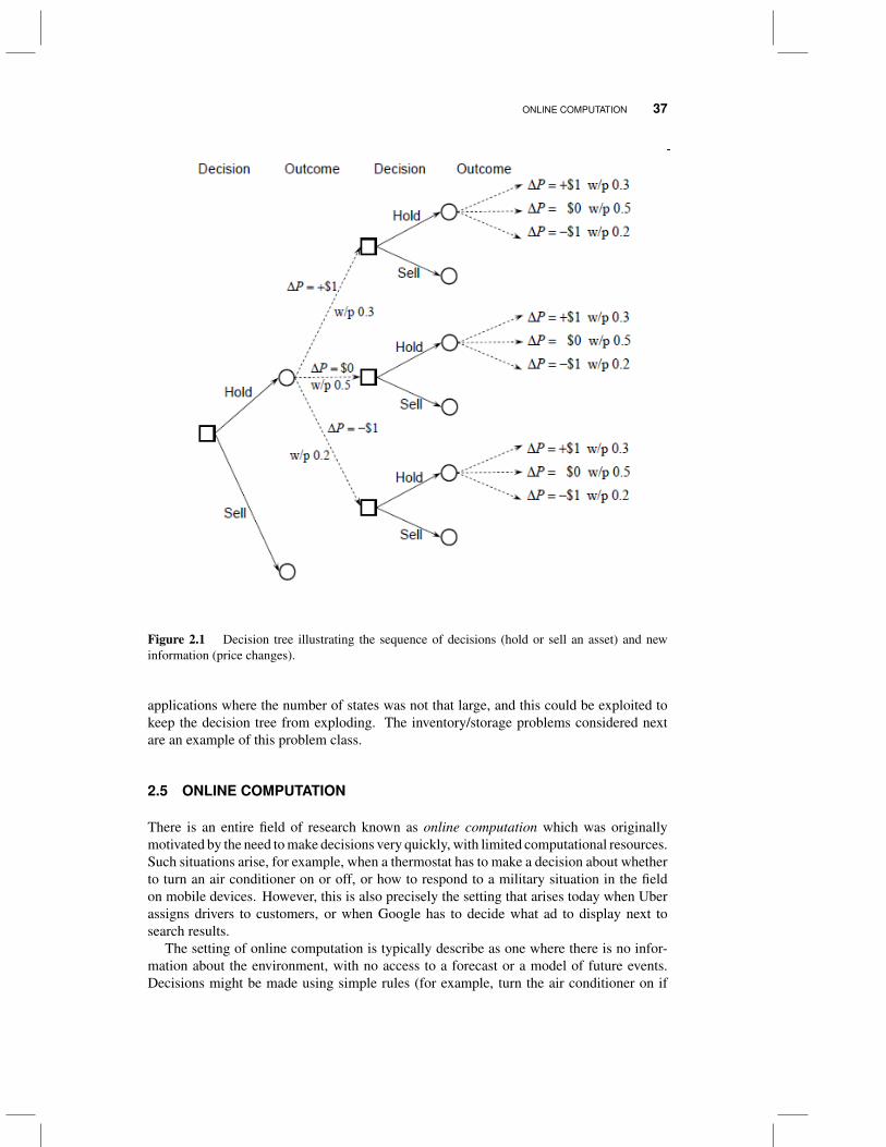
Decision trees are easily one of the most familiar ways to depict sequential decision prob-lems, with or without uncertainty. Figure 2.1 illustrates a simple problem of determiningwhether to hold or sell an asset. If we decide to hold, we observe changes in the price ofthe asset and then get to make the decision of holding or selling.

Figure 2.1 illustrates the basic elements of a decision tree. Square nodes representpoints where decisions are made, while circles represent points where random informationis revealed. We solve the decision tree by rolling backward, calculating the value of beingat each node. At an outcome now, we average across all the downstream nodes (sincewe do not control which node we transition to), while at decision nodes, we pick the bestdecision based on the one-period reward plus the downstream value.

Almost any dynamic program with discrete states and actions can be modeled as adecision tree. The problem is that they are not practical when there are a large numberof states, actions and random outcomes, since the tree grows extremely quickly. Thebreakthrough known as “dynamic programming” was the recognition that there were many

ONLINE COMPUTATION 37

3

Figure 2.1 Decision tree illustrating the sequence of decisions (hold or sell an asset) and newinformation (price changes).

applications where the number of states was not that large, and this could be exploited tokeep the decision tree from exploding. The inventory/storage problems considered nextare an example of this problem class.

2.5 ONLINE COMPUTATION

There is an entire field of research known as online computation which was originallymotivated by the need to make decisions very quickly, with limited computational resources.Such situations arise, for example, when a thermostat has to make a decision about whetherto turn an air conditioner on or off, or how to respond to a military situation in the fieldon mobile devices. However, this is also precisely the setting that arises today when Uberassigns drivers to customers, or when Google has to decide what ad to display next tosearch results.

The setting of online computation is typically describe as one where there is no infor-mation about the environment, with no access to a forecast or a model of future events.Decisions might be made using simple rules (for example, turn the air conditioner on if


the temperature is greater than 72 degrees F, and turn it off when it falls to 70 degrees F).Alternatively, we might look at a section of actions (such as picking Uber drivers to servea customer) where we want to pick the best action. Let C(St, x) be the cost of choosingdriver x in a set Xt (the eight closest drivers), which depends on the state St. We mightchoose the best driver by solving

xt = arg minx∈Xt

C(St, x).

The online computation community will insist that they cannot make decisions thatconsider the impact on the future because they do not know anything about the future. Theresearch community likes to prove bounds on the regret, which quantifies how much betteryou might do with perfect information about the future.

2.6 TWO-STAGE STOCHASTIC PROGRAMMING

Imagine that we have a problem where we have to decide how many Christmas trees toplant which will determine our inventory five years into the future. Call this decisionx0 (we suppress the year we are planning for), which may be a vector determining theplantings at different wholesalers around a region. Then, when we arrive at the sales year(five years later), we see the demand D1 for Christmas trees and the prices p1 that theretailers are willing to pay and then have to make shipping decisions x1 to each retailer. LetW1 = (D1, p1) represent this random information, and let ω refer to a sample realizationofW1, so thatW1(ω) = (D1(ω), p1(ω)) is one possible realization of demands and prices.We make the decision x1 after we see this information, so we have a decision x1(ω) foreach possible realization. Assume that c0 is the costs of producing trees at each location,and c1 are the costs associated with the vector x1.

Assume for the moment that Ω = (ω1, ω2, . . . , ωK) is a (not too large) set of possibleoutcomes for the demand D1(ω) and price p1(ω). A standard way of writing this problemis in the form

maxx0

(−c0x0 +

∑ω∈Ω

p(ω) maxx1:x1(ω)≤b1(ω)−A1x0

((p1(ω)− c1)x1(ω)

)). (2.8)

In the language of stochastic programming, the second state decision variables, x1(ω),are called “recourse variables” since they represent the “recourse” as information becomesknown. Two-stage stochastic programs are basically deterministic optimization problems,but they can be very large deterministic optimization problems, albeit ones with specialstructure.

For example, imagine that we allow the first stage decision x0 to “see” the informationin the second stage, in which case we would write it as x0(ω). In this case, we obtain aseries of smaller problems, one for each ω. However, now we are allowing x0 to cheat byseeing into the future. We can overcome this by introducing a nonanticipativity constraintwhich might be written

x0(ω)− x0 = 0.

Now, we have a family of first stage variables x0(ω), one for each ω, and then a singlevariablex0, where we are trying to force eachx0(ω) to be the same (at which point we wouldsay that x0 is “nonanticipative”). Algorithmic specialists can exploit the nonanticipacity

CHANCE CONSTRAINED PROBLEMS 39

constraint by relaxing it, then solving a series of smaller problems (perhaps in parallel),and then introducing linking mechanisms so that the overall procedure converges toward asolution that satisfies the nonanticipativity constraint.

2.7 CHANCE CONSTRAINED PROBLEMS

There are problems where we have to satisfy a constraint that depends on uncertain infor-mation at the time we make a decision. For example, we may wish to allocate inventorywith the goal that we cover demand 80 percent of the time. Alternatively, we may wish toschedule a flight so that it is on time 90 percent of the time. We can state these problemsusing the general form

minxf(x), (2.9)

subject to the probabilistic constraint (often referred to as a chance constraint)

P[C(x,W ) ≥ 0] ≤ α. (2.10)

The constraint (2.10) is often written in the equivalent form

P[C(x,W ) ≤ 0] ≥ 1− α. (2.11)

Here, C(x,W ) is the amount that a constraint is violated (if positive). Using our examples,it might be the demand minus the inventory which is the lost demand if positive, or thecovered demand if negative. Or, it could be the arrival time of a plane minus the scheduledtime, where positive means a late arrival.

Chance constrained programming is a method for handling a particular class of con-straints that involve uncertainty, typically in the setting of a static problem: make decision,see information, stop. Chance constrained programs convert these problems into deter-ministic, nonlinear programs, with the challenge of computing the probabilistic constraintwithin the search algorithm.

2.8 SHORTEST PATHS

Shortest path problems represent a particularly elegant and powerful problem class, sincea node in the network can represent any discrete state, while links out of the node canrepresent a discrete action.

2.8.1 A deterministic shortest path problem

A classical sequential decision problem is the shortest path problem. Let

I = The set of nodes (intersections) in the network,L = The set of links (i, j) in the network,cij = The cost (typically the time) to drive from node i to node j,

i, j ∈ I, (i, j) ∈ L,

I+i = The set of nodes j for which there is a link (i, j) ∈ L,I−j = The set of nodes i for which there is a link (i, j) ∈ L.


Step 0. Let

v0j =

M j 6= r,0 j = r.

where “M” is known as “big-M” and represents a large number. Let n = 1.

Step 1. Solve for all i ∈ I,

vni = minj∈I+i

(cij + vn−1

j

).

Step 2. If vni < vn−1i for any i, let n = n+ 1 and return to step 1. Else stop.

Figure 2.2 A basic shortest path algorithm.

A traveler at node i needs to choose the link (i, j) where j ∈ I+i is a downstream node

from node i. Assume that the traveler needs to get from an origin node q to a destinationnode r at least cost. Let

vj = The minimum cost required to get from node j to node r.

We can think of vj as the value of being in state j. At optimality, these values will satisfy

vi = minj∈I+i

(cij + vj

).

This fundamental equation underlies all the shortest path algorithms used in our GPSdevices, although these have been heavily engineered to achieve the rapid response wehave become accustomed to. A basic shortest path algorithm is given in 2.2, although thisrepresents just the skeleton of what a real algorithm would look like.

Shortest path problems represent particularly attractive instances of dynamic program-ming problems because the state space is just the set of intersections describing a network.Even though there may be millions of intersections describing large networks such as thosein the U.S., Europe and other major regions, this is still quite manageable (production algo-rithms use different heuristics to restrict the search). Finding the best path across a complextransportation network will seem like a toy after we consider some of the multidimensionalproblems that arise in other applications.

2.8.2 A stochastic shortest path problem

We are often interested in shortest path problems where there is uncertainty in the cost oftraversing a link. For our transportation example, it is natural to view the travel time on alink as random, reflecting the variability in traffic conditions on each link.

There are situations where the costs or times are random. To handle this new dimensioncorrectly, we have to specify whether we see the outcome of the random cost on a linkbefore or after we make the decision whether to traverse the link. If we assume that wesee the cost on a link cij while we are at node i, but before we have decided if we want totraverse to node j, then we would write our dynamic programming recursion using

vni = E

minj∈I+i

(cij(W ) + vn−1

j

).

OPTIMAL STOPPING 41

Here, the expectation is outside of the min operator that chooses the best decision, capturingthe fact that now the decision itself is random.

Note that our notation is ambiguous, in that with the same notation, we have twovery different models. In chapter 9, we are going to refine our notation so that it willbe immediately apparent when a decision “sees” the random information and when thedecision has to be made before the information becomes available.

2.9 OPTIMAL STOPPING

A classical problem in stochastic optimization is known as the optimal stopping problem.Imagine that we have a stochastic process Wt (this might be prices of an asset) whichdetermines a reward f(Wt) if we stop at time t (the price we receive if we stop and sell theasset). Let ω ∈ Ω be a sample path of W1, . . . ,WT (we are going to limit our discussionto finite horizon problems, which might represent a maturation date on a financial option).Let

Xt(ω) =

1 If we stop at time t,0 Otherwise.

Let τ be the time t when Xt = 1 (we assume that Xt = 0 for t > τ ). This notation createsa problem, because ω specifies the entire sample path, which seems to suggest that we areallowed to look into the future before making our decision at time t (don’t laugh - thismistake is not just easy to make, it is actually a fairly standard approximation in the fieldof stochastic programming where.

To fix this, we require that the function Xt be constructed so that it depends only on thehistory W1, . . . ,Wt. When this is the case τ is called a stopping time. The optimizationproblem can then be stated as

maxτ

EXτf(Wτ ), (2.12)

where we require τ to be a “stopping time.” Mathematicians will often express this byrequiring that τ (or equivalently, Xt) be an “Ft-measurable function.” This language isfamiliar to students with training in measure-theoretic probability, which is not necessaryfor developing models and algorithms for stochastic optimization. Later, we are going toprovide an easy introduction to these ideas (in chapter 9, and then explain why we do notneed to use this vocabulary.

More practically, the way we are going to solve the stopping problem in (2.12) is thatwe are going to create a function Xπ(St) that depends on the state of the system at timet. For example, imagine that we need a policy for selling an asset. Let Rt = 1 if we areholding the asset, and 0 otherwise. Assume that p1, p2, . . . , pt is the history of the priceprocess, where we receive pt if we sell at time t. Further assume that we create a smoothedprocess pt using

pt = (1− α)pt−1 + αpt.

At time t, our state variable is St = (Rt, pt, pt). A sell policy might look like

Xπ(St|θ) =

1 If pt > θmax or pt < θmin,0 Otherwise.


Finding the best policy means finding the best θ = (θmin, θmax) by solving

maxθ

ET∑t=0

ptXπ(St|θ).

Our stopping time, then, is the earliest time τ = t where Xπ(St|θ) = 1.Optimal stopping problems arise in a variety of settings. Some examples include:

American options - An American option on a financial asset gives you the right to sellthe asset at the current price on or before a specified date.

Machine replacement - While monitoring the status of a (typically complex) piece ofmachinery, we need to create a policy that tells us when to stop and repair or replace.

Homeland security - The National Security Administration collects information on manypeople. The NSA needs to determine when to start tracking someone, when to stop(if they feel the target is of no risk) or when to act (when they feel the target is ofhigh risk).

Health intervention - Public health officials are continually tracking the presence of dis-ease in a population. They need to make the call when a pattern of occurrencesconstitutes an actionable outbreak.

Optimal stopping may look like a disarmingly easy problem, given the simplicity of thestate variable. However, in real applications there is almost always additional informationthat needs to be considered. For example, our asset selling problem may depend on a basketof indices or securities that greatly expands the dimensionality of the state variable. Themachine replacement problem might involve a number of measurements that are combinedto make a decision. The homeland security application could easily involve a number offactors (places the person has visited, the nature of communications, and recent purchases).Finally, health decisions invariably depend on a number of factors that are unique to eachpatient.

2.10 MARKOV DECISION PROCESSES

Assume that our system is described a set of discrete states s ∈ S = 1, 2, . . . , |S|, anddiscrete actions a ∈ A (which might depend on the state that we are in, in which case wemight write As). Further assume we receive a reward r(s, a) if we take action a while instate s. Finally (and this is the strongest assumption) assume that we are given a set oftransition probabilities

P (s′|s, a) = The probability that state St+1 = s′ given that we are in state St = s and takeaction a.

If we are solving a finite horizon problem, let Vt(St) be the optimal value of being instate St and behaving optimally from time t onward. If we are given Vt+1(St+1), we cancompute Vt(St) using

Vt(St) = maxa∈As

(r(St, a) +

∑s′∈S

P (s′|St, a)Vt+1(s′)). (2.13)

REINFORCEMENT LEARNING 43

Equation (2.13) may seem somewhat obvious, but when first introduced it was actually quitea breakthrough, and is known as Bellman’s optimality equation in operations research andcomputer science, or Hamilton-Jacobi equations in control theory (although this communitytypically writes it for deterministic problems).

Equation (2.13) is the foundation for a major class of policies that we refer to as policiesbased on value function (or VFA policies), recognizing that if we can actually compute(2.13), then the value function is optimal, giving us a rare instance of an optimal policy.

If the one-step transition matrix P (s′|St, a) can be computed (and stored), then equation(2.13) is quite easy to compute starting at time T (when we assume VT (ST ) is given, whereit is fairly common to useVT (ST ) = 0). Perhaps for this reason, there has been considerableinterest in this community on steady state problems, where we assume that as t→∞, thatVt(St)→ V (S). In this case, (2.13) becomes

V (s) = maxa∈As

(r(s, a) +

∑s′∈S

P (s′|s, a)V (s′). (2.14)

Now we have a system of equations that we have to solve to find V (s). We review thesemethods in some depth in chapter 14.

Bellman’s equation was viewed as a major computational breakthrough when it was firstintroduced, because it avoids the exploision of decision trees. Quickly, however, people(including Bellman) realized that there was a problem when the state s is a vector (evenif it is still discrete). The size of the state space grows exponentially with the number ofdimensions, typically limiting this method to problems where the state variable has at mostthree or four dimensions.

Bellman’s equation actually suffers from three curses of dimensionality. In additionto the state variable, the random information (buried in the one-step transition P (s′|s, a))might also be a vector. Finally, the action a might be a vector x. It is common for peopleto dismiss “dynamic programming” (but they mean discrete Markov decision processes)because of “the curse of dimensionality” (they could say because of “the curses of dimen-sionality”), but the real issue is the use of lookup tables. There are strategies for overcomingthe curses of dimensionality, but if it were easy, this would be a much shorter book.

2.11 REINFORCEMENT LEARNING

Reinforcement learning evolved out of efforts to model animal behavior, as with mice tryingto find their way through a maze to a reward (see figure 2.3). Successes were learned overtime by capturing the probability that a path from a particular point in the maze eventuallyleads to a success. This work was started in the early 1980’s by Rich Sutton and hisacademic adviser Andy Barto. At some point, people realized that the central ideas couldall be cast in the language of Markov decision processes, but without the use of backwarddynamic programming that are implied in the calculation of equation (2.13) above. Insteadof stepping backward in time, reinforcement learning proceeds by stepping forward intime, but then performing backward updates. These ideas became the foundation of whatlater became known as approximate (or adaptive) dynamic programming. The process ofstepping forward avoids the need to loop over all possible states, as is required if solvingequation (2.14).

Despite the similarities between reinforcement learning and what we will later introduceas approximate dynamic programming, the reinforcement learning community had its rootsin a particular class of problems. For example, the prototypical reinforcement learning


Figure 2.3 Finding a path through a maze.

problem is “model free” which means that we do not have access to the one-step transitionmatrix P (s′|s, a) which is considered a fundamental input to a Markov decision process.Instead, we assume that if we are in a state St and take an action at, that we would thenobserve St+1 without having access to the equations that describe how we get there.

Instead of learning the value V (s) of being in a state s, the core algorithmic strategy ofreinforcement learning involves learning the value Q(s, a) of being in a state s and thentaking an action a. The basic algorithm, known as Q-learning, proceedings by computing

qn(sn, an) = r(sn, an) + λmaxa′

Qn−1(s′, a′), (2.15)

Qn(sn, an) = (1− αn−1)Qn−1(sn, an) + αn−1qn(sn, an). (2.16)

To compute (2.15), we assume we are given a state sn. We then use some method to choosean action an, which produces a reward r(sn, an). We then randomly sample a downstreamstate s′ that might result from being in a state sn and taking action an. Using our simulateddownstream state s′, we then find what appears to be the best action a′ based on our currentestimates Qn−1(s′, a′) (known as ”Q-factors”). We then update the estimates of the valueof being in states sn and action an. When this logic is applied to our maze in figure 2.3,the algorithm steadily learns the state/action pairs with the highest probability of findingthe exit, but it does require sampling all states and actions often enough.

There are many variations of Q-learning that reflect different rules for choosing thestate sn, choosing the action an, what is done with the updated estimate qn(sn, an), andhow the estimates Qn(s, a) are calculated (equations (2.15) - (2.16) reflect a lookup tablerepresentation). These basic equations would only work for problems with relatively smallstates and actions, which means we could simply use equation (2.13) if we know the one-step transition matrix (hence we see why this community typically assumes that we do notknow the transition matrix).

OPTIMAL CONTROL 45

2.12 OPTIMAL CONTROL

The optimal control community is most familiar with the deterministic form of a controlproblem, which is typically written in terms of the “system model” (transition function)

xt+1 = f(xt, ut),

where xt is the state variable and ut is the control. The problem is to find ut that solves

minu

T∑t=0

L(xt, ut) + JT (xT ), (2.17)

where L(x, u) is a “loss function” and JT (xT ) is a terminal cost (the notation here is notstandard).

A solution strategy which is so standard that it is often stated as part of the model isto view the transition xt+1 = f(xt, ut) as a constraint that can be relaxed, producing theobjective

minu

T∑t=0

(L(xt, ut) + λt(xt+1 − f(xt, ut))

)+ JT (xT ), (2.18)

where λt is a set of Lagrange multipliers known as “co-state variables.” The function

H(x0, u) =

T∑t=0

(L(xt, ut) + λt(xt+1 − f(xt, ut))

)+ φT (xT )

is known as the Hamiltonian.The most common stochastic version would be written

xt+1 = f(xt, ut, wt)

where wt is random at time t. Often, wt is viewed as a form of additive noise that ariseswhen trying to measure the state of the system, which consists of the location and speed ofan aircraft. In this setting, the noise is additive, and would be written

xt+1 = f(xt, ut) + wt.

When we introduce noise, we can still write the objective as (2.17), but now we have tofollow the objective function with the statement “where ut is Ft-measurable” (see section9.10.2 for an explanation of this term). The problem with this formulation is that it doesnot provide an immediate path to computation. As readers will see, the way this problemis solved is to construct a policy, that we denote (using the notation of this example) byUπ(xt), which means the function has to determine a decision ut = Uπ(xt) using onlythe information in the state xt. The search for solution that satisfies the requirement that“ut be Ft-measurable” is the same as finding some function that depends on xt (which inturn can only depend on information that has arrived before time t). A significant part ofthis book is focused on describing methods for finding these functions.


2.13 MULTI-STAGE STOCHASTIC PROGRAMMING

The stochastic programming community, which works primarily with the two-stage for-mulation given in section 2.6, likes to formulate sequential (called “multi-stage”) linearprograms using

minA0x0=b0x0≥0

〈c0, x0〉+ E

minB0x0+A1x1=b1

x1≥0

〈c1, x1〉+ E

· · ·+E

minBT−1xT−1+AT xT=bT

xT≥0

〈cT , xT 〉

. . . . (2.19)

Equation (2.19) captures the nesting of decisions (which are minimized) and information(represented by the expectations). This formulation assumes that xt is a vector which hasto satisfy constraints of the form Atxt = bt, where At, bt and ct are all random (at time 0).

Equation (2.19) is equivalent to

minx0∈X0(S0)

C(S0, x0) + E[

minx1∈X1(S1)

C(S1, x1) + E[· · ·+ E

[min

xT∈XT (ST )C(ST , xT )

]. . .

]],

(2.20)

which is closer to our canonical form. We build on (2.20) in chapter 19 which exploitsthe convexity of each minimization problem. We then return to (2.19) in chapter 20 wherewe show how the stochastic programming community builds approximate policies using alookahead model.

This formulation can look quite frightening. Later, we are going to describe severalsolution strategies that are well suited to providing good solutions (even if they are notoptimal) that work for the setting of vector-valued decisions xt.

2.14 THE NOMADIC TRUCKER

There is an industry called truckload trucking, where a single truck driver will pick up aload at A, drive it from A to B, drop it off at B, and then has to look for a new load (thereare places to call in to get a list of available loads). The driver has to think about how muchmoney he will make moving the load, but he then also has to recognize that the load willmove him to a new city. The driver is characterized at each point in time by his current orfuture location `t (which is a region of the country), his equipment type Et which is thetype of trailer he is pulling (which can change depending on the needs of the freight), hisestimated time of arrival at `t (denoted by τeta), and the time τt that he has been away fromhis home (which is fixed, so we exclude it from the state variable). We roll these attributesinto a vector rt given by

rt = (`t, Et, τeta, τhomet ).

When the driver arrives at the destination of a load, he calls a freight broker and gets a setof loads Lt that he can choose from. This means that his state variable (the informationjust before he makes a decision), is given by

St = (rt,Lt).

STATISTICS AND MACHINE LEARNING 47

The driver has to choose among a set of actionsAt = (Lt, “hold”) that includes the loadsin the set Lt, or doing nothing. Once the driver makes this choice, the set Lt is no longerrelevant. His state immediately after he makes his decision is called the post-decision stateSat = rat , which is updated to reflect the destination of the load, and the time he is expectedto arrive at this location.

The natural way for a driver to choose which action to take is to balance the contributionof the action, which we write asC(St, at), and the value of the driver in his “post-decision”state rat . We might write this policy, which we call Aπ(St), using

Aπ(St) = arg maxa∈At

(C(St, a) + V at (rat )

).

The algorithmic challenge is creating the estimates V at (rat ), which is an example of whatwe will call a value function approximation. If the number of possible values of the driverattribute vector rat was not too large, we could solve this problem using the same way wewould solve the stochastic shortest path problem introduced in section 2.8.2. The hiddenassumption in this problem is that the number of nodes is not too large (even a millionnodes is considered manageable). When a “node” is a multidimensional vector rt, then wemay have trouble manipulating all the possible values this may take (another instances ofthe curse of dimensionality).

2.15 STATISTICS AND MACHINE LEARNING

There are close parallels between stochastic optimization and machine learning. Let:

xn = The data corresponding to the nth instances of a problem (the characteristicsof a patient, the attributes of a document, the data for an image) that we wantto use to predict an outcome yn,

yn = The response, which might be the response of a patient to a treatment, thecategorization of a document, or the classification of an image,

f(xn|θ) = Our model which we use to predict yn given xn,θ = An unknown parameter vector used to determine the model.

We assume we have some metric that indicates how well our model f(x|θ) is performing.For example, we might use

L(xn, yn|θ) = (yn − f(xn|θ))2.

The function f(x|θ) can take on many forms. The simplest is a basic linear model ofthe form

f(x|θ) =∑f∈F

θfφf (x),

where φf (x) is known as a feature, and F is the set of features. There may be just ahandful of features, or thousands. The statistics and machine learning communities havedeveloped a broad array of functions, each of which is parameterized by some vector θ(often designated as weights w). We review these in some depth in chapter 3.

The most typical optimization problem in machine learning is to use a batch dataset tosolve the nonlinear problem

minθ

1

N

N∑n=1

(yn − f(xn|θ))2.


For problems where the dimensionality of θ is in the thousands, this can be a difficultalgorithmic challenge.

There is a separate class of machine learning problems that involve working with datathat arrives over time, a field that is known as online learning. For this setting, weindex our sequence of data and observations as x0, y1, x1, y2, . . . , xn, yn+1. This indexingcommunicates the property that we see xn before observing yn+1. In this case, we wouldlet θn be our estimate of θ based on the data (x0, y1, . . . , xn). There are a variety ofalgorithms that we will later describe as policies Θπ(Sn) which maps what we know asof time n (in theory this could be the entire history, but typically it is more compact) toproduce a parameter estimate θn to be used to predict yn+1. Now we have the problem ofdesigning policies, which is the focus of most of this book.

2.16 A SIMPLE MODELING FRAMEWORK FOR DYNAMIC PROGRAMS

Now that we have covered a number of simple examples, it is useful to briefly review theelements of a dynamic program. We are going to revisit this topic in considerably greaterdepth in chapter 9, but this discussion provides a brief introduction. Our presentationfocuses on stochastic dynamic programs which exhibit a flow of uncertain information.These problems, at a minimum, consist of the following elements:

The state variable - This captures all the information we need to make a decision, as wellas the information that we need to describe how the system evolves over time.

The decision variable - Decisions/actions represent how we control the process.

Exogenous information - This is data that first becomes known each time period (forexample, the demand for product, or the price at which it can be purchased or sold).In addition, we also have to be told the initial state of our system.

The transition function - This function determines how the system evolves from the stateSt to the stateSt+1 given the decision that was made at time t and the new informationthat arrived between t and t+ 1.

The objective function - This function specifies the costs being minimized, or the contri-butions/rewards being maximized, over time horizon.

We can illustrate these elements using the simple asset acquisition problem from section8.3.6.

The state variable is the information we need to make a decision and compute functionsthat determine how the system evolves into the future. In our asset acquisition problem,we need three pieces of information. The first is Rt, the resources on hand before wemake any decisions (including how much of the demand to satisfy). The second is thedemand itself, denoted Dt, and the third is the price pt. We would write our state variableas St = (Rt, Dt, pt).

We have two decisions to make. The first, denoted xDt , is how much of the demand Dt

during time interval t that should be satisfied using available assets, which means that werequire xDt ≤ Rt. The second, denoted xOt , is how many new assets should be acquired attime t which can be used to satisfy demands during time interval t+ 1.

The exogenous information process consists of three types of information. The first isthe new demands that arise during time interval t, denoted Dt. The second is the change

A SIMPLE MODELING FRAMEWORK FOR DYNAMIC PROGRAMS 49

in the price at which we can sell our assets, denoted pt. Finally, we are going to assumethat there may be exogenous changes to our available resources. These might be blooddonations or cash deposits (producing positive changes), or equipment failures and cashwithdrawals (producing negative changes). We denote these changes by Rt. We oftenuse a generic variable Wt to represent all the new information that is first learned duringtime interval t, which for our problem would be written Wt = (Rt, Dt, pt). In additionto specifying the types of exogenous information, for stochastic models we also have tospecify the likelihood of a particular outcome. This might come in the form of an assumedprobability distribution for Rt, Dt, and pt, or we may depend on an exogenous source forsample realizations (the actual price of the stock or the actual travel time on a path).

Once we have determined what action we are going to take from our decision rule,we compute our contribution Ct(St, xt) which might depend on our current state and theaction xt that we take at time t. For our asset acquisition problem (where the state variableis Rt), the contribution function is

Ct(St, xt) = ptxDt − ctxOt .

In this particular model, Ct(St, xt) is a deterministic function of the state and action. Inother applications, the contribution from action xt depends on what happens during timet+ 1.

Next, we have to specify how the state variable changes over time. This is done using atransition function which we might represent in a generic way using

St+1 = SM (St, xt,Wt+1),

where St is the state at time t, xt is the decision we made at time t and Wt+1 is ourgeneric notation for the information that arrives between t and t+ 1. We use the notationSM (·) to denote the transition function, where the superscript M stands for “model” (or“system model” in recognition of vocabulary that has been in place for many years in theengineering community). The transition function for our asset acquisition problem is givenby

Rt+1 = Rt − xDt + xOt + Rt+1,

Dt+1 = Dt − xDt + Dt+1,

pt+1 = pt + pt+1.

This model assumes that unsatisfied demands are held until the next time period.Our final step in formulating a dynamic program is to specify the objective function.

Assume we are trying to maximize the total contribution received over a finite horizont = (0, 1, . . . , T ). If we were solving a deterministic problem, we might formulate theobjective function as

max(xt)Tt=0

T∑t=0

Ct(St, xt). (2.21)

We would have to optimize (2.21) subject to a variety of constraints on the actions(x0, x1, . . . , xT ).

If we have a stochastic problem, which is to say that there are a number of possiblerealizations of the exogenous information process (Wt)

Tt=0, then we have to formulate the

objective function in a different way. If the exogenous information process is uncertain,


we do not know which state we will be in at time t. Since the state St is a random variable,then the choice of decision (which depends on the state) is also a random variable.

We get around this problem by formulating the objective in terms of finding the bestpolicy (or decision rule) for choosing decisions. A policy tells us what to do for all possiblestates, so regardless of which state we find ourselves in at some time t, the policy willtell us what decision to make. This policy must be chosen to produce the best expectedcontribution over all outcomes. If we let Xπ(St) be a particular decision rule indexed byπ, and let Π be a set of decision rules, then the problem of finding the best policy would bewritten

maxπ∈Π

ET∑t=0

Ct(St, Xπ(St)). (2.22)

Exactly what is meant by finding the best policy out of a set of policies is very problemspecific. Our decision rule might be to order Xπ(Rt) = S − Rt if Rt < s and orderXπ(Rt) = 0 if Rt ≥ s. The family of policies is the set of all values of the parameters(s, S) for s < S (here, s and S are parameters to be determined, not state variables). Ifwe are selling an asset, we might adopt a policy of selling if the price of the asset pt fallsbelow some value p. The set of all policies is the set of all values of p. However, policiesof this sort tend to work only for very special problems.

Equation (2.22) states our problem as one of finding the best policy (or decision rule,or function Xπ) to maximize the expected value of the total contribution over our horizon.There are a number of variations of this objective function. For applications where thehorizon is long enough to affect the time value of money, we might introduce a discountfactor γ and solve

maxπ∈Π

ET∑t=0

γtCt(St, Xπ(St)). (2.23)

There is also considerable interest in infinite horizon problems of the form

maxπ∈Π

E∞∑t=0

γtCt(St, Xπ(St)). (2.24)

Equation (2.24) is often used when we want to study the behavior of a system in steadystate.

Equations such as (2.22), (2.23), and (2.24) are all easy to write on a sheet of paper.Solving them computationally is a different matter. That challenge is the focus of this book.

A complete specification of a dynamic program requires that we specify both data andfunctions, as follows:

Data:

– The initial state S0.

– The exogenous information process Wt. We need to know what information isarriving from outside the system, and how it is being generated. For example,we might be given the probability of an outcome, or given a process that createsthe data for us.

Functions:

BIBLIOGRAPHIC NOTES 51

– The contribution function C(St, xt). This may be specified in the formC(St, xt,Wt+1). In this case, we may need to compute the expectation, orwe may work directly with this form of the contribution function.

– The transition function SM (St, xt,Wt+1).

– The family of decision functions (Xπ(S))π∈Π.

This description provides only a taste of the richness of sequential decision processes.Chapter 9 describes the different elements of a dynamic program in far greater detail.

2.17 BIBLIOGRAPHIC NOTES

• Section xx -

canonical problems - princeton...

Documents