Can viewer proximity be a behavioural marker forAutism Spectrum Disorder?

R. Bishain∗, B. Chakrabarti†, J. Dasgupta§, I. Dubey†‡, Sharat Chandran∗[On behalf of the START consortium.]

∗ Department of Computer Science and Engineering, Indian Institute of Technology Bombay, India† Centre for Autism, School of Psychology & Clinical Language Sciences, University of Reading, UK

‡ Division of Psychology, De Montfort University, UK§ Child Development Group, Sangath, Bardez, Goa, India

Abstract—Screening for any of the Autism Spectrum Disordersis a complicated process often involving a hybrid of behaviouralobservations and questionnaire based tests. Typically carried outin a controlled setting, this process requires trained cliniciansor psychiatrists for such assessments. Riding on the wave oftechnical advancement in mobile platforms, several attempts havebeen made at incorporating such assessments on mobile andtablet devices.

In this paper we analyse videos generated using one suchscreening test. This paper reports the first use of the efficacyof using the observer’s distance from the display screen whileadministering a sensory sensitivity test as a behavioural markerfor Autism for children aged 2-7 years. The potential for usinga test such as this in casual home settings is promising.

I. INTRODUCTION

Autism Spectrum Disorders (ASD) are associated [1] withatypical social communicative behaviour, restricted range ofinterests and repetitive behaviour. While the global population-level prevalence of ASD is estimated to be around 1%, thechallenges faced in low and middle income countries (LMIC)are significantly greater than those faced by high incomecountries (HIC) due to the shortage of resources and expertise.Assessment of ASD constitutes the first hurdle in meeting thisimportant global health need.

Patients going to the hospital, even assuming the availabilityof trained professionals is not scalable. In 2018, Egger et al.[2]reported the use of an iPad based method to be used in ahome setting in HIC; from the computer vision perspective,the technology of interest was to automatically obtain headpose based on the method in [3] and emotion and attentionanalysis [4].

These autism screening and diagnostic analyses typicallyfocus on social functioning measures. However, many autisticindividuals show an atypical sensory sensitivity in one or moremodalities [5]. Indeed, recognition of this gap in assessmentsled to sensory symptoms being included within the diagnosticframework for ASD in the latest version [1] of the diagnosticmanual. The sensory sensitivity test in this paper follows ideassimilar to [2] but includes the ‘wheel-task’(Sec. I-A) and isadministered in LMIC on casual Android platforms.

The problem solved in this paper is illustrated in Figure 1(refer next page). To the best of our knowledge, this is the firstevidence of using a computer vision algorithm for the wheel

task for a significant medical condition, with emphasis that thetarget audience is children in a relaxed LMIC home setting.

A. The wheel task

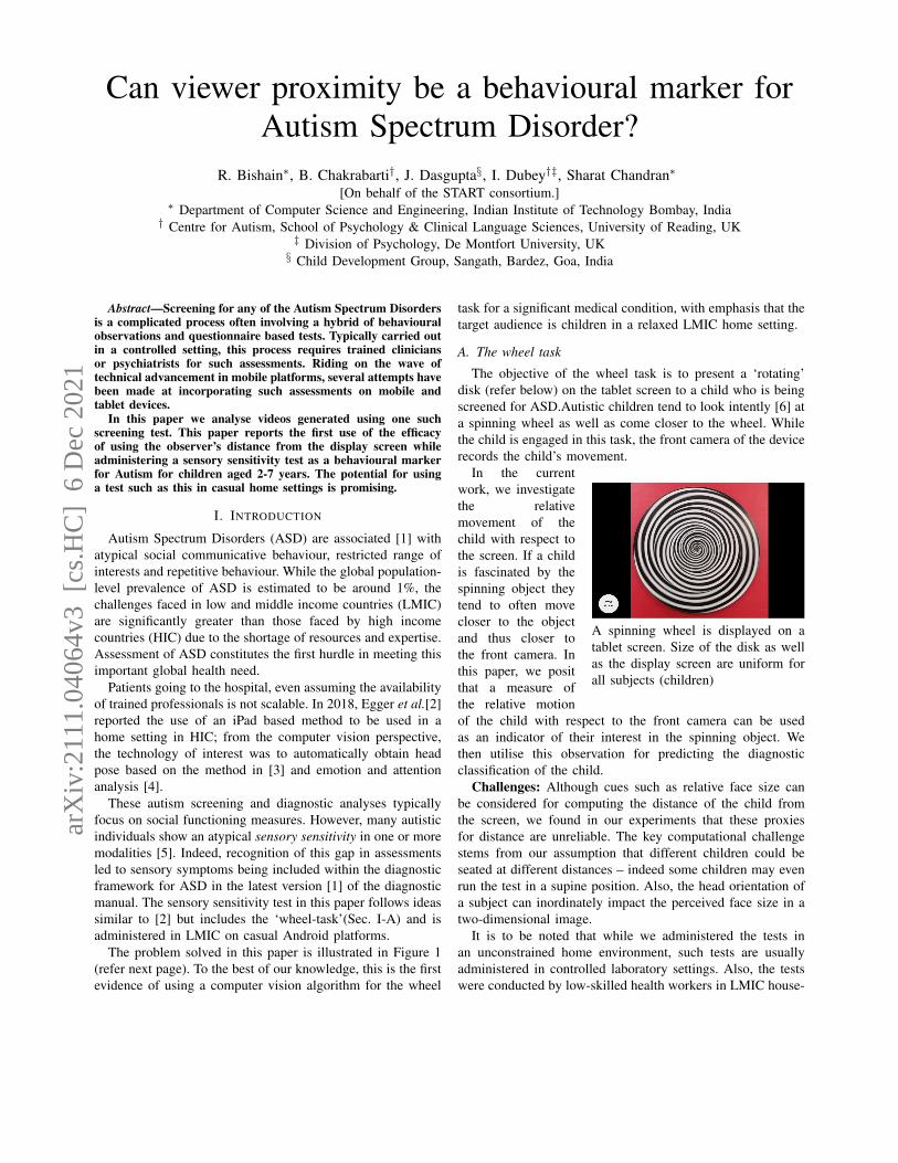
The objective of the wheel task is to present a ‘rotating’disk (refer below) on the tablet screen to a child who is beingscreened for ASD.Autistic children tend to look intently [6] ata spinning wheel as well as come closer to the wheel. Whilethe child is engaged in this task, the front camera of the devicerecords the child’s movement.

A spinning wheel is displayed on atablet screen. Size of the disk as wellas the display screen are uniform forall subjects (children)

In the currentwork, we investigatethe relativemovement of thechild with respect tothe screen. If a childis fascinated by thespinning object theytend to often movecloser to the objectand thus closer tothe front camera. Inthis paper, we positthat a measure ofthe relative motionof the child with respect to the front camera can be usedas an indicator of their interest in the spinning object. Wethen utilise this observation for predicting the diagnosticclassification of the child.

Challenges: Although cues such as relative face size canbe considered for computing the distance of the child fromthe screen, we found in our experiments that these proxiesfor distance are unreliable. The key computational challengestems from our assumption that different children could beseated at different distances – indeed some children may evenrun the test in a supine position. Also, the head orientation ofa subject can inordinately impact the perceived face size in atwo-dimensional image.

It is to be noted that while we administered the tests inan unconstrained home environment, such tests are usuallyadministered in controlled laboratory settings. Also, the testswere conducted by low-skilled health workers in LMIC house-

arX

iv:2

111.

0406

4v3

[cs

.HC

] 6

Dec

202

1

Fig. 1: Overview: The contribution in this paper is to provide (and validate) a method of obtaining viewer distances forchildren whose pictures are taken in a casual home setup with uncalibrated low resolution cameras and utilise it for diagnosticclassification of autism.

holds. The workers were not provided any special training, un-like the clinicians who usually conduct the tests in controlledsettings. Hence, our approach addresses this constrained con-text and aims to capture the viewer’s proximity using imagescaptured from an uncalibrated low resolution camera. Pleasesee the supplementary video on the data capture.

B. Contributions

Tablets recording viewers is becoming increasingly com-mon, to say the least, and face identification is standard. Thekey technical contributions in this work are

• A method that computes in metric units the distancebetween the front camera of a tablet and the face of ahuman being. This measure is often a requirement in suchdiagnostic analyses. (The source code will be provided)

• A method that works– for children as they tend to get distracted quickly

and may not remain stationary in front of the tabletdevice during the task.

– in poorly lit conditions as the study is aimed at chil-dren from less privileged backgrounds. (Methods thatwork in well-lit homes may not generalise across lowresolution, poorly lit environments. In this paper, wedemonstrate evidence that current computer visionmethods are quite robust in home settings.)

• Quantitative evidence that viewer proximity in the wheeltask can be a marker for classification in child develop-ment. (All earlier work on this task were subjective lab-based assessments. We report the first classifier whichutilises this measure for diagnostic classification).

The rest of this paper is organised as follows. We firstdiscuss related work, and follow it up with the methodsuggested and its validation (Section II). Results are presentedin Section III.

C. Related Work

Since ASD is a spectrum of developmental disorders, mostof the diagnostic and screening assessments revolve aroundthe analysis of behavioural symptoms. These can be anal-ysed in dyadic interaction between the subject and others.For instance, in the case of young children, by observing

the interaction between mother and child, psychologists candevise an appropriate intervention plan (i.e., therapy) for betterparental care and child development.

In such assessments [7] the aim is to capture importantbehavioural cues such as shared mutual attention, imitatingother’s actions, etc. Such play interactions are also analysedfor screening and diagnostics [8] purposes and for longitudinalimpact assessments [9] of the selected intervention therapy.

Researchers have tried to employ machine vision techniquesto automate such analysis but they are either dependent on amultimodal setup or analyse a very structured set of actionsunder a constrained paradigm. For instance, Rehg et al.[10]have analysed behaviour of children by creating an indepen-dent Rapid-ABC paradigm. In contrast, Marinoiu et al.[11]have attempted both action and emotion recognition tasks in anunstaged environment. However, they have focused on robotassisted therapy and not on the diagnostic aspect of autismwhich is the focus of our paper.

The analysis of head movement, while children performautism specific assessments, has gained traction in the com-puter vision community in recent years. More specifically,Martin et al.[12] contrasted head movements between ASDand non ASD groups of children when watching videos ofsocial vs non-social stimuli. They have studied group differ-ences vis-a-vis pitch, yaw and roll of the head movements.Ogihara et al.[13] studied specific temporal patterns of headmovements to understand their diagnostic potential.

The studies based on head movement [12] and [13], dis-cussed above, have been carried out in laboratory settings.Children are seated in front of a monitor, with a mountedcamera, which records their movement while they view variousstimuli on the screen. In contrast, our work relies solelyon videos captured at the home of participant children. Thevideos are captured from the relatively weak front camera(0.35 Megapixels) of Android tablet devices while the childrenview the stimuli presented on the tablet screen.

II. METHODOLOGY

The complete process pipeline, from data capture in theform of videos, to the final diagnostic class prediction, isdepicted diagrammatically in Figure 1. The details of each

phase in the process pipeline are elaborated in Sections II-Ato II-C.

A. Data CollectionAs mentioned, several tasks are administered in determining

markers for autism. Typically, the battery of incorporated tasksare carried out in controlled settings in a laboratory withexpensive setups, sensors and trackers. In contrast, we arelimited in our approach due to the requirements of a low-resource setting. Due to this requirement the data collectionwas performed using an economical tablet device with addi-tional limitations of:

• No user dependence is permitted (For example, no taskor user specific calibration was allowed).

• No separate recording – the recording was only via a lowresolution RGB front camera that could be triggered withthe task.

• No additional user sensors or wearable setup was allowed.These limitations are to be contrasted with prior work.

The tasks were conducted by non-specialist community healthworkers on young children at their homes. This was essentialfor the desired scalability and for collecting data on autismrelated symptoms in LMIC. In summary, the task was admin-istered in as natural a setting as possible. In this paper, wehave focused only on one of the several tasks which havebeen incorporated for screening of autism risk.

Diagnostic Category Video Count Videos Used(TD) Typically Developing 39 37(ASD) Autism Spectrum Disorder 43 41(ID) Intellectually Disabled 39 37Total 121 115

TABLE I: Number of wheel task videos collected across thediagnostic categories of TD, ASD and ID children. All datacollected on the same device model. Maximum video durationwas 80 seconds. As per our knowledge this is the largestdataset for such a task captured in home settings

The data is a set of videos of children performing the wheeltask. Prior to the data collection the children were categorisedin one of the three diagnostic groups by experts in a prestigiousmedical school-cum-hospital-cum-medical research universitythat sees a daily footfall of over thousand patients of allages. In contrast, the video data set is collected by minimallytrained workers who have administered these tasks in semi-urban households. A corpus of 121 videos has been created(with 195000 image frames). The videos have been capturedacross the diagnostic categories or classes of TD (TypicallyDeveloping), ASD and ID (Intellectual Disability) children asshown in Table I.

These videos were manually verified for usability in ourtask and some videos were observed to be unusable due toinsufficient length of relevant footage. Finally, after removingsuch videos a total of 115 videos were used for this analysiswith the respective distribution across the three diagnosticclasses as shown in Table I. We have included a sample videofrom this dataset in the supplementary material.

B. Viewer proximity algorithm

As its input, the algorithm receives a video of a userwatching a tablet screen as captured from the front camera.The intrinsic (or extrinsic) camera parameters are unknown. Asits output the algorithm predicts the user’s distance (in metricunits) from the tablet screen in each video frame. There is noexpectation that the user will be in a seated position, or inany fixed position. It is conceivable that the user may not bevisible while the task is going on since children can be easilydistracted.

The length, denoted bythe arrowheads, repre-sent the bitragion breadth([14], page 188).

First we detected the face, andthen landmarks within the faceusing a state-of-the-art deep neu-ral network-based face detector(FAN) [15]. This detector pro-vides, for each frame in the video,a reference 3D value for eachlandmark in a local coordinatesystem. However, these 3D co-ordinates, while valid for eachframe, are incomparable acrossframes. Next, a reference frame istherefore desirable, and we usedthe frame corresponding to the“most frontal”1 face amongst allfaces in the video.

The unifying factor across allthese frames is, of course, the camera. Since the 2D landmarkfor each corresponding 3D landmark is available (indeed,that’s how the 3D is estimated in the first place), we were ableto use these correspondences to find the camera centre. Oncethe camera centre is computed, it is relatively straightforwardto compute the metric distance to one of the landmarks, suchas the left or the right eye. The data from this step is used inablation Scheme 2 described later.

As communicated by domain experts, some child develop-ment studies rely on actual Euclidean distance values. Sincefrom a single camera, we cannot obtain Euclidean (metric)values, we use the concept of “bitragion breadth” – the widthbetween the two tragions (cartilaginous notches at the frontof the ear). Once the head pose is calculated in pixel units,we obtain the average depth in real units using the scalefactor from the bitragion breadth of children. The benchmarkbitragion breadth is taken to be 10.6 cm corresponding tothe 50th percentile bitragion breadth for children, both malesand females (obtained from [14], page 454). While the headsizes do vary across children, the variation is insignificant inchildren in our data set who primarily belong in a narrow agerange.

1) Algorithm Correctness: To validate our approach weneed reliable ground truth values for viewer distance from thetablet screen. This ground truth can then be used for validatingthe results output by our proximity estimation algorithm. Wefollowed two different approaches for validation. The first

1Details provided in the supplementary material

approach relied on manually noting the distances for eachframe while the second approach relied on a Kinect V2 basedannotation setup. Here, we discuss validation using the Kinectdevice based on the setup shown in Figure 2a (both approachesrevealed similar results). In the setup we have placed the tabletdevice at a distance of 90 cm from the Kinect.

Calibrating Kinect: During the validation process we ob-served that Kinect prediction in the near camera range was notreliable (During the wheel task children typically tend to watchthe screen at a range of 20 − 50 cm from the tablet device.Kinect predictions were first manually verified to be stableand reliable in the 60+ cm range (hence the 90 cm distancementioned above). More details about Kinect calibration areincluded in the supplementary material.

(a) Setup

(b) Validation.

Fig. 2: (a) Representative depiction of the Kinect setup tovalidate the correctness of our algorithm. The actual compu-tation does not use the Kinect. (b) Distance in cm vs the framenumber. Our results mimic those of the Kinect. The differencein the estimate in (b) is due to the pixel scaling factor usedin our approach which assumes a small child’s head while thevalidations were performed on adults.

Validating the algorithm: The output of a sample test runon this validation set up is depicted in Figure 2b. In the setup,the viewer is looking at the mobile screen and is initially 30cm away from it. The viewer moves back up to a distance of50 cm away from the mobile before returning to the startingpoint. Note that this translates to a corresponding distance of118.5 and 138.5 cm in the setup, respectively (refer Figure 2a).

Although they follow the same trend, as shown in Figure2b, the distance predicted by our approach do not match the

ground truth (values predicted by Kinect). This is expectedas the predictions are derived from an assumed bitragionbreadth of 10.6 cm which is typically the value for an averagechild (the corresponding size for an average adult would beconsiderably higher. The validation tests were performed byadults). The predicted depth values are filtered (to smoothenout and remove the noise in prediction) before being used fordiagnostic classification.

(a) Typically Developing category

(b) Autism Spectrum Disorder category

Fig. 3: Distance in cm vs frame number of the video. Thesefigures show the motion of a child’s head relative to thetablet screen while performing the wheel task from our viewerproximity estimation algorithm.

C. Training

In this section, we describe the process of analysing theviewer movement data in order to predict the diagnosticclassification. We utilise the data output by our proximityestimation algorithm as described in Section II-B.

Preprocessing: As is evident from Figure 3a and Figure 3bthe movement data is now reduced to a vector containing theestimated distance of the child from the tablet for each frameof the recorded video. The size of the vector depends on howlong the task was undertaken (a stop button is provided on thescreen for the child). It can range from a few hundred datapoints to a maximum of 2400 data points (recall that videosin the task are displayed for no more than 80 seconds).

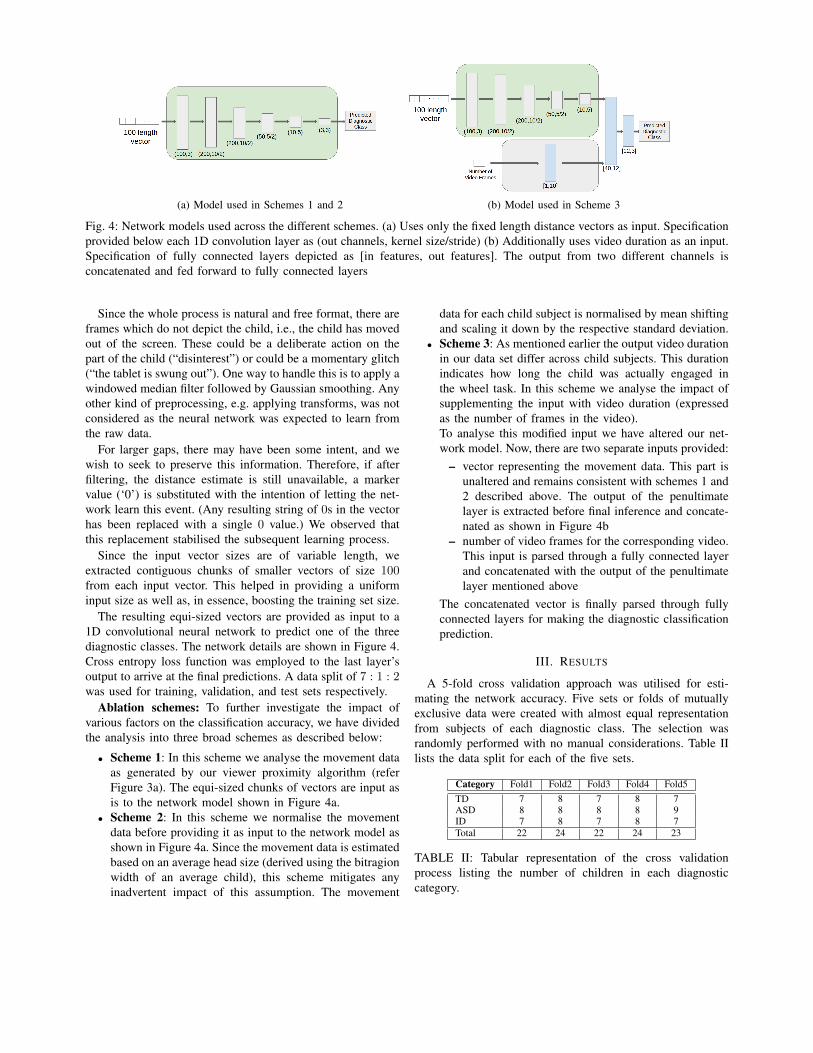
(a) Model used in Schemes 1 and 2 (b) Model used in Scheme 3

Fig. 4: Network models used across the different schemes. (a) Uses only the fixed length distance vectors as input. Specificationprovided below each 1D convolution layer as (out channels, kernel size/stride) (b) Additionally uses video duration as an input.Specification of fully connected layers depicted as [in features, out features]. The output from two different channels isconcatenated and fed forward to fully connected layers

Since the whole process is natural and free format, there areframes which do not depict the child, i.e., the child has movedout of the screen. These could be a deliberate action on thepart of the child (“disinterest”) or could be a momentary glitch(“the tablet is swung out”). One way to handle this is to apply awindowed median filter followed by Gaussian smoothing. Anyother kind of preprocessing, e.g. applying transforms, was notconsidered as the neural network was expected to learn fromthe raw data.

For larger gaps, there may have been some intent, and wewish to seek to preserve this information. Therefore, if afterfiltering, the distance estimate is still unavailable, a markervalue (‘0’) is substituted with the intention of letting the net-work learn this event. (Any resulting string of 0s in the vectorhas been replaced with a single 0 value.) We observed thatthis replacement stabilised the subsequent learning process.

Since the input vector sizes are of variable length, weextracted contiguous chunks of smaller vectors of size 100from each input vector. This helped in providing a uniforminput size as well as, in essence, boosting the training set size.

The resulting equi-sized vectors are provided as input to a1D convolutional neural network to predict one of the threediagnostic classes. The network details are shown in Figure 4.Cross entropy loss function was employed to the last layer’soutput to arrive at the final predictions. A data split of 7 : 1 : 2was used for training, validation, and test sets respectively.

Ablation schemes: To further investigate the impact ofvarious factors on the classification accuracy, we have dividedthe analysis into three broad schemes as described below:

• Scheme 1: In this scheme we analyse the movement dataas generated by our viewer proximity algorithm (referFigure 3a). The equi-sized chunks of vectors are input asis to the network model shown in Figure 4a.

• Scheme 2: In this scheme we normalise the movementdata before providing it as input to the network model asshown in Figure 4a. Since the movement data is estimatedbased on an average head size (derived using the bitragionwidth of an average child), this scheme mitigates anyinadvertent impact of this assumption. The movement

data for each child subject is normalised by mean shiftingand scaling it down by the respective standard deviation.

• Scheme 3: As mentioned earlier the output video durationin our data set differ across child subjects. This durationindicates how long the child was actually engaged inthe wheel task. In this scheme we analyse the impact ofsupplementing the input with video duration (expressedas the number of frames in the video).To analyse this modified input we have altered our net-work model. Now, there are two separate inputs provided:

– vector representing the movement data. This part isunaltered and remains consistent with schemes 1 and2 described above. The output of the penultimatelayer is extracted before final inference and concate-nated as shown in Figure 4b

– number of video frames for the corresponding video.This input is parsed through a fully connected layerand concatenated with the output of the penultimatelayer mentioned above

The concatenated vector is finally parsed through fullyconnected layers for making the diagnostic classificationprediction.

III. RESULTS

A 5-fold cross validation approach was utilised for esti-mating the network accuracy. Five sets or folds of mutuallyexclusive data were created with almost equal representationfrom subjects of each diagnostic class. The selection wasrandomly performed with no manual considerations. Table IIlists the data split for each of the five sets.

Category Fold1 Fold2 Fold3 Fold4 Fold5TD 7 8 7 8 7ASD 8 8 8 8 9ID 7 8 7 8 7Total 22 24 22 24 23

TABLE II: Tabular representation of the cross validationprocess listing the number of children in each diagnosticcategory.

In each of the five rounds, a different hold out set waschosen from among the five sets. The hold out set was usedfor testing the model which was trained (and validated) on theremaining 4 sets. Throughout the five rounds a consistent splitof 7 : 1 was maintained between the training and validationsets.

Note that a naive classifier, which stubbornly outputs onlyone class for any subject, would have achieved a maximumclassification accuracy of 35.65% (= 41/115). A randomscheme would get one out of 3 right (33%).

It is to be noted that the network has been trained forpredicting the label for smaller equi-sized input vectors. Thefinal classification for a subject (child) was arrived at byconsidering the modal value of the predictions for all theconstituent smaller vectors for that subject. The resultingprediction accuracies of the models, for the correspondingschemes, have been noted for each of the five rounds asshown in Figure 5. Please note that the average accuracy isarrived at by weighting the round’s accuracy by the size ofthe corresponding hold out set (i.e., number of subjects in thehold out set).

We observe that Scheme 2 provides better resultscompared to the other schemes. It can be noted thatnormalizing the estimated viewer proximity values en-hances the overall classification accuracy to 68.69%. Fur-ther, we present the confusion matrix for one of the5 folds of the experiment for Scheme 2. Here, thecolumns represent the predicted values for a given class.

Category TD ASD IDTD 6 2 0ASD 0 8 0ID 2 2 4

Similar confusionmatrices for theremaining folds usedfor cross-validationhave been includedin the supplementarymaterial.

IV. CONCLUSION

Finding behavioural markers for ASD is a challengingproposition. Nearly all prior work in this direction have onlybeen experimented in a laboratory or a clinic setup. It isdesirable if the hospital comes to the child but such a setupposes interesting challenges. This process becomes even moredifficult if the hospital comes to the child in the form of amobile device that has “tasks”.

In this paper, we analysed the “wheel task” in which thefront camera of the device is used to record a child watchinga “spinning” wheel. To the best of our knowledge, such ananalysis has not been performed in the casual setting of a semi-urban home in LMIC countries. We used the viewer proximityas a marker for ASD, and we observed that we could correctlyclassify a child solely with this measure with an averageaccuracy of 68.69%. Although this may not seem like a strongresult when compared to classification tasks in other domains,it is the first such attempt for this task. Such tasks are usuallycarried out in lab settings, where the analysis is subjective.

(a) Scheme 1

(b) Scheme 2

(c) Scheme 3

Fig. 5: Accuracy results for the different analysis schemes

Further, our results may be seen as a weak classifier which canassist in such analyses. It is also worth noting that this accuracyis significantly higher than that of a naive classifier. We areable to achieve this through a computer vision algorithm thatmeasures viewer proximity in casual video recordings.

V. ACKNOWLEDGEMENT

The START (Screening Tools for Autism Risk usingTechnology) consortium members are listed alphabetically:Bhismadev Chakrabarti, Debarati Mukherjee, Gauri Divan,Georgia Lockwood-Estrin, Indu Dubey, Jayashree Dasgupta,Mark Johnson, Matthew Belmonte, Rahul Bishain, SharatChandran, Sheffali Gulati, Supriya Bhavnani, Teodora Gliga,Vikram Patel. This work was funded by a Medical ResearchCouncil Global Challenge Research Fund grant to the STARTconsortium (PI: Chakrabarti; Grant ID: MR/P023894/1).

REFERENCES

[1] Diagnostic and statistical manual of mental disorders, 5th ed., AmericanPsychiatric Association, 2013.

[2] H. L. Egger, G. Dawson, J. Hashemi, K. L. Carpenter, S. Espinosa,K. Campbell, S. Brotkin, J. Schaich-Borg, Q. Qiu, M. Tepper, J. P. Baker,R. A. Bloomfield, and G. Sapiro, “Automatic emotion and attentionanalysis of young children at home: a ResearchKit autism feasibilitystudy,” NPJ Digital Medicine, vol. 1, no. 1, pp. 1–10, 2018.

[3] X. Xiong and F. De la Torre, “Supervised descent method and itsapplications to face alignment,” in CVPR, 2013, pp. 532–539.

[4] J. Hashemi, K. Campbell, K. L. Carpenter, A. Harris, Q. Qui, M. Tepper,S. Espinosa1, B. J. S., S. Marsan, R. Calderbank, J. Baker, H. L. Egger,G. Dawson, and G. Sapiro, “A scalable app for measuring autism riskbehaviours in young children,” in MOBIHEALTH, 2015.

[5] S. Baron-Cohen, E. Ashwin, C. Ashwin, T. Tavassoli, andB. Chakrabarti, “Talent in autism: hyper-systemizing, hyper-attentionto detail and sensory hypersensitivity,” Philosophical Transactionsof the Royal Society B: Biological Sciences, vol. 364, no. 1522, pp.1377–1383, 2009.

[6] T. Tavassoli, K. Bellesheim, P. M. Siper, A. T. Wang, D. Halpern,M. Gorenstein, and J. D. Buxbaum, “Measuring sensory reactivity inautism spectrum disorder: application and simplification of a clinician-administered sensory observation scale.” Journal of Autism and Devel-opmental Disorders, vol. 46, no. 1, pp. 287–293, 2016.

[7] S. Freeman and C. Kasari, “Parent–child interactions in autism: Char-acteristics of play,” Autism, vol. 17, no. 2, pp. 147–161, 2013.

[8] J. M. Guercio and A. D. Hahs, “Applied behavior analysis and the autismdiagnostic observation schedule (ADOS): A symbiotic relationship foradvancements in services for individuals with autism spectrum disorders(ASDs),” Behavior analysis in practice, vol. 8, no. 1, pp. 62–65, 2015.

[9] A. Pickles, A. Le Couteur, K. Leadbitter, E. Salomone, R. Cole-Fletcher,H. Tobin, I. Gammer, J. Lowry, G. Vamvakas, S. Byford, and C. Alfred,“Parent-mediated social communication therapy for young children withautism (PACT): long-term follow-up of a randomised controlled trial,”The Lancet, vol. 388, no. 10059, pp. 2501–2509, 2016.

[10] J. Rehg, G. Abowd, A. Rozga, M. Romero, M. Clements, S. Sclaroff,I. Essa, O. Ousley, Y. Li, C. Kim, and H. Rao, “Decoding children’ssocial behavior,” in CVPR, 2013, pp. 3414–3421.

[11] E. Marinoiu, M. Zanfir, V. Olaru, and C. Sminchisescu, “3D humansensing, action and emotion recognition in robot assisted therapy ofchildren with autism,” in CVPR, 2018, pp. 2158–2167.

[12] K. B. Martin, Z. Hammal, G. Ren, J. F. Cohn, J. Cassell, M. Ogihara,J. C. Britton, A. Gutierrez, and D. S. Messinger, “Objective measurementof head movement differences in children with and without autismspectrum disorder,” Molecular Autism, vol. 9, no. 1, p. 14, 2018.

[13] M. Ogihara, Z. Hammal, K. B. Martin, J. F. Cohn, J. Cassell, G. Ren,and D. S. Messinger, “Categorical timeline allocation and alignmentfor diagnostic head movement tracking feature analysis,” in CVPRWorkshops, 2019, pp. 43–51.

[14] R. G. Snyder, L. W. Schneider, L. O. Clyde, M. R. Herbert,D. H. Golomb, and M. A. Schork, “Anthropometry of infants,children, and youths to age 18 for product safety design. finalreport.” 1977, last accessed: Apr 2020. [Online]. Available: https://math.nist.gov/∼SRessler/anthrokids/child77lnk.pdf

[15] A. Bulat and G. Tzimiropoulos, “How far are we from solving the2D & 3D face alignment problem?(and a dataset of 230,000 3D faciallandmarks),” in ICCV, 2017, pp. 1021–1030.

I. SUPPLEMENTARY MATERIAL

A. Sample Videos

Please refer to the attached video files for a demonstration

1) Sample wheel task video: This attached video pro-vides an example of the video of a child performing the wheeltest in a home setting. Please note that the video has beenmodified to protect the privacy of the participant. (For instance,the yellow box is added to detect and subsequently blur thechild’s face).

2) START A field data collection app for autism screening:The wheel test is one of several assessments which are usedfor screening. We collected data on various other tests bytaking a tablet directly to households. Like the wheel test,these assessments too are part of an app which is installed on

the tablet. For context, we provide this attached video

B. Kinect Calibration

Kinect depth prediction values were not in centimeter units.We have arrived at the correlation between the Kinect pre-dicted depth values to the actual distance in cm, as shown inFigure 1. To arrive at this relation both the Kinect device anda plane object were kept on a level surface. The object wasthen kept at various distances in the 90-120 cm range fromthe Kinect. The predicted Kinect depth is plotted against theactual object distance to arrive at the approximation given bythe following formula y = 1.91x+ 581, where y is the depthof the object as predicted by Kinect, and x is the ground truthobserved distance of the object.

Fig. 1: Correlation between Kinect predicted depth values andthe actual distance in cm. The Y-axis represents the depthvalue as predicted by Kinect. The corresponding ground truthobserved distance is plotted on the X-axis. This correlation isused to convert the Kinect predictions to the actual distancein centimetres.

C. Deriving most frontal face

In this section we provide the steps to determine the framewith the most ‘frontal’ face in a video. The intention is to

(a) 2D facial landmarks

(b) 3D facial landmarks

Fig. 2: Plots of (a) 2D and (b) 3D facial landmarks used toarrive at the most frontal face

capture the image frame in which the user’s face tends to bemost upright and parallel to the image plane.

The following steps are performed for arriving at the mostfrontal face:

Input: 68 facial landmarks as shown in Figure 2 for eachframe

Output: Frame number with the most frontal faceCalculation steps:1) For each image frame in the video:

a) Mean shift the landmarks (using mean of thelandmarks in the current frame)

b) Scale each landmark down by its correspondingmagnitude

c) Obtain the (absolute) depth difference for oppositelandmark point pairs on the jaw-line (landmarkpoint pairs – 1:17, 2:16, 3:15, ...8:10). Select themaximum ‘depth difference’ for this image framefrom these values

2) From among the frames having ±4 degree ‘eyelineorientation’, select the min(max(depth difference)). i.e.Note the frame with with minimum of the maximumdepth difference calculated in step 1c above.For calculation of ‘eyeline orientation’ the steps are:

arX

iv:2

111.

0406

4v3

[cs

.HC

] 6

Dec

202

1

a) Obtain centroid of eyes (centroid of landmarkpoints 37-42 and 43-48)

b) Obtain eyeline orientation as the slope of the linejoining the two eye centroids

D. Confusion Matrices

We present the confusion matrix for each of the five foldsbelow (see main paper for description) for Scheme 2 here.Note that the precision and recall value for each fold isindicated in the last row and column, respectively of thecorresponding fold. As before, columns represent the predictedvalues for a given class.

The overall precision and recall values have been depictedin Table VI

Category TD ASD ID RecallTD 5 0 2 0.71ASD 0 7 2 0.78ID 0 3 4 0.57Precision 1 0.7 0.5

TABLE I: Fold 1 confusion matrixCategory TD ASD ID RecallTD 6 2 0 0.75ASD 0 8 0 1ID 2 2 4 0.5Precision 0.75 0.67 1

TABLE II: Fold 2 confusion matrixCategory TD ASD ID RecallTD 5 1 1 0.71ASD 3 5 0 0.63ID 1 1 5 0.71Precision 0.56 0.71 0.83

TABLE III: Fold 3 confusion matrixCategory TD ASD ID RecallTD 4 2 2 0.5ASD 0 7 1 0.88ID 0 4 4 0.5Precision 1 0.54 0.57

TABLE IV: Fold 4 confusion matrixCategory TD ASD ID RecallTD 6 1 0 0.86ASD 0 7 1 0.88ID 1 4 2 0.29Precision 0.86 0.58 0.67

TABLE V: Fold 5 confusion matrixCategory TD ASD ID Average RecallTD 26 6 5 0.7ASD 3 34 4 0.83ID 4 14 19 0.51Average Precision 0.79 0.63 0.68

TABLE VI: Overall Precision and Recall

E. Mean reciprocal rank (MRR)

We report an average MRR of 0.83 for the five folds forScheme 2. The MRR values for individual folds are as shownbelow in Table VII

Fold No. 1 2 3 4 5 OverallMRR 0.826 0.792 0.818 0.854 0.833 0.825

TABLE VII: Mean Reciprocal Rank for Scheme 2