can the total solar days (epoch jan 0, 1980) - sidc.be 4 meteo/dudokdewit_tsi.pdf · can the total...

Can the Total Solar Irradiance be reconstructed from solar activity proxies ?

T. Dudok de Wit1, M. Kretzschmar1, J. Lilensten2, P.-O. Amblard3, S. Moussaoui4, J. Aboudarham5, F. Auchère6

1 LPCE, Orléans, 2 LPG, Grenoble, 3 GIPSAlab, Grenoble, 4 IRCCYN, Nantes, 5 LESIA, Paris, 6 IAS, Orsay

SOLAR IRRADIANCE VARIABILITY 9

Year

1363

1364

1365

1366

1367

1368

1369

So

lar

Irra

dia

nce

(W

m!

2)

78 80 82 84 86 88 90 92 94 96 98 00 02 04 Year

1363

1364

1365

1366

1367

1368

1369

So

lar

Irra

dia

nce

(W

m!

2)

0 2000 4000 6000 8000

Days (Epoch Jan 0, 1980)

HF

AC

RIM

I

HF

AC

RIM

I

HF

AC

RIM

II

VIR

GO

Average minimum: 1365.560 ± 0.009 Wm!2

Difference between minima: !0.016 ± 0.007 Wm!2

Cycle amplitudes: 0.933 ± 0.019; 0.897 ± 0.020; 0.824 ± 0.017 Wm!2

0.1%

Figure 9. Shown is the final version of the PMOD composite. Compared to the earlierversions the maximum of cycle 21 is at about the level as before, but has less noise,especially in the early part. This may indicate that the early HF corrections have indeedbeen improved. Finally, the difference between the minima has also not changed. The datesof the maxima are 26/03/1979 – 25/12/1981, 28/04/1989 – 21/02/1992 and 19/01/2000 –18/02/2003 and of the minima 13/04/1985 – 07/06/1987 and 05/05/1995 – 02/08/1997.

et al., 1995) and is shown in Figure 9. The differences to the earlier versions

have been shown in the Figures 4 and 7 and lie more in the details than in the

overall behaviour. Thus the final result does not change the trend or the amplitudes

significantly. Overall it is a more reliable time series mainly due to the fact that the

corrections of the different records are based on the same type of model.

!1

0

1

2

56

!1

0

1

20 2000 4000 6000 8000

Days (Epoch Jan 0, 1980)

a) PMOD r2 = 0.8324

slope: 0.000 ± 0.0044 µWm!2a!1

difference of minima: !0.0074 ± 0.0387 Wm!2

!1

0

1

2

56

!1

0

1

2

b) ACRIM r2 = 0.6185

slope: 0.242 ± 0.0066 µWm!2a!1

difference of minima: 0.5608 ± 0.0402 Wm!2

Year

!1

0

1

2

56

78 79 80 81 82 83 84 85 86 87 88 89 90 91 92 93 94 95 96 97 98 99 00 01 02 03 Year

!1

0

1

2

r2 = 0.6308

slope: 0.264 ± 0.0064 µWm!2a!1

c) IRMB

difference of minima: 0.2214 ± 0.0421 Wm!2

Diffe

ren

ce

in

Wm

!2 o

f C

om

po

site

! K

itt!

Pe

ak r

eco

nstr

ucte

d

Figure 10. The comparison of the three composites with a reconstruction of TSI fromKitt-Peak magnetograms by Wenzler (2005)

ISSI2005a_CF.tex; 9/03/2006; 21:54; p.9

C. Fröhlich & J. Lean (2006)

ESSW4, Brussels, Nov. 2007

The Sun and the Earth’s Climate 27

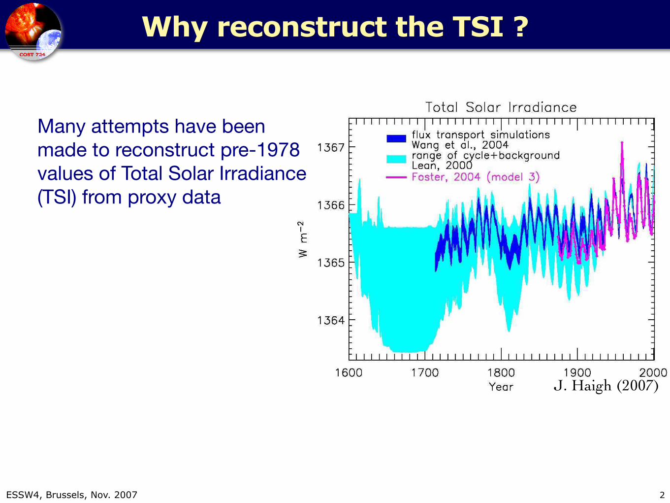
Figure 22: Reconstructions by various authors of total solar irradiance over the past 400 years.From Judith Lean, based on data from Wang et al. (2005); Lean (2000); Foster (2004).

5 Solar spectral irradiance

The interaction of solar radiation with the atmosphere is fundamental in determining its temper-ature structure and in controlling many of the chemical processes which take place there. Thissection outlines the role of solar UV radiation in determining the budget of stratospheric ozone anddiscusses how the composition and thermodynamic structure of the stratosphere are modulated bysolar variability. It goes on to consider how perturbations to the stratosphere may impact solarradiative forcing of tropospheric climate.

5.1 Absorption of solar spectral radiation by the atmosphere

Absorption by the atmosphere of solar radiation depends on the concentrations and spectral prop-erties of the atmospheric constituents. Figure 23 shows a blackbody spectrum at 5750 K, repre-senting solar irradiance at the top of the atmosphere, and a spectrum of atmospheric absorption.Absorption features due to specific gases are clear with molecular oxygen and ozone being themajor absorbers in the ultraviolet and visible regions and water vapour and carbon dioxide moreimportant in the near-infrared.

Clearly the flux at any point in the atmosphere depends on the properties and quantity ofabsorbing gases at higher altitudes and on the path length for the radiation, taking into accountthe solar zenith angle. The heights at which most absorption takes place at each wavelengthcan be seen in Figure 24 which shows the altitude of unit optical depth for an overhead Sun.At wavelengths shorter than 100 nm most radiation is absorbed at altitudes between 100 and200 km by atomic and molecular oxygen and nitrogen, mainly resulting in ionized products. SolarLyman-! radiation at 121.6 nm penetrates to the upper mesosphere where it makes a significantcontribution to heating rates and water vapour photolysis. Between about 80 and 120 km oxygen isphoto-dissociated as it absorbs in the Schumann–Runge continuum between 130 and 175 nm. TheSchumann–Runge bands, 175 – 200 nm, are associated with electronic plus vibrational transitions

Living Reviews in Solar Physicshttp://www.livingreviews.org/lrsp-2007-2

Why reconstruct the TSI ?

Many attempts have been made to reconstruct pre-1978 values of Total Solar Irradiance (TSI) from proxy data

2

J. Haigh (2007)


The Sun and the Earth’s Climate 27

Figure 22: Reconstructions by various authors of total solar irradiance over the past 400 years.From Judith Lean, based on data from Wang et al. (2005); Lean (2000); Foster (2004).

5 Solar spectral irradiance

The interaction of solar radiation with the atmosphere is fundamental in determining its temper-ature structure and in controlling many of the chemical processes which take place there. Thissection outlines the role of solar UV radiation in determining the budget of stratospheric ozone anddiscusses how the composition and thermodynamic structure of the stratosphere are modulated bysolar variability. It goes on to consider how perturbations to the stratosphere may impact solarradiative forcing of tropospheric climate.

5.1 Absorption of solar spectral radiation by the atmosphere

Absorption by the atmosphere of solar radiation depends on the concentrations and spectral prop-erties of the atmospheric constituents. Figure 23 shows a blackbody spectrum at 5750 K, repre-senting solar irradiance at the top of the atmosphere, and a spectrum of atmospheric absorption.Absorption features due to specific gases are clear with molecular oxygen and ozone being themajor absorbers in the ultraviolet and visible regions and water vapour and carbon dioxide moreimportant in the near-infrared.

Clearly the flux at any point in the atmosphere depends on the properties and quantity ofabsorbing gases at higher altitudes and on the path length for the radiation, taking into accountthe solar zenith angle. The heights at which most absorption takes place at each wavelengthcan be seen in Figure 24 which shows the altitude of unit optical depth for an overhead Sun.At wavelengths shorter than 100 nm most radiation is absorbed at altitudes between 100 and200 km by atomic and molecular oxygen and nitrogen, mainly resulting in ionized products. SolarLyman-! radiation at 121.6 nm penetrates to the upper mesosphere where it makes a significantcontribution to heating rates and water vapour photolysis. Between about 80 and 120 km oxygen isphoto-dissociated as it absorbs in the Schumann–Runge continuum between 130 and 175 nm. TheSchumann–Runge bands, 175 – 200 nm, are associated with electronic plus vibrational transitions

Living Reviews in Solar Physicshttp://www.livingreviews.org/lrsp-2007-2

Why reconstruct the TSI ?

Many attempts have been made to reconstruct pre-1978 values of Total Solar Irradiance (TSI) from proxy data

2

J. Haigh (2007)

Such reconstruction are needed to

assess solar effects on past climate changes

understand what causes the weak variability of the TSI


How to reconstruct the TSI

Most reconstructions of the TSI use solar activity indices: sunspot number, MgII index, ...

short-time reconstructions (days) have been quite successful so far...

...but the (presumably important) role of the solar magnetic field is hard to include

3

ESSW4, Brussels, Nov. 2007 4J. Lean, Physics Today, 2005


There is a problem...

before determining HOW to reconstruct the TSI from proxies

we need to

determine IF this reconstruction can be done at all

and

and WHICH proxies are the best model inputs

5

6

AGRICULTURE

APPROPRIATIONS

INTERNATIONAL RELATIONS

BUDGET

HOUSE ADMINISTRATION

ENERGY/COMMERCE

FINANCIAL SERVICES

VETERANS’ AFFAIRS

EDUCATION

ARMED SERVICES

JUDICIARY

RESOURCES

RULES

SCIENCE

SMALL BUSINESS

OFFICIAL CONDUCTTRANSPORTATION

GOVERNMENT REFORM

WAYS AND MEANS

INTELLIGENCE

HOMELAND SECURITY

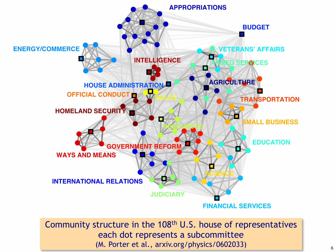
FIG. 4: (Color) Network of committees (squares) and subcommittees (circles) in the 108th

U.S. House of Representatives, color-coded by the parent standing and select committees. (The

depicted labels indicate the parent committee of each group but do not identify the location of

that committee in the plot.) As with Fig. 2, this visualization was produced using a variant of the

Kamada-Kawai spring embedder, with link strengths (again indicated by darkness) determined by

normalized interlocks. Observe again that subcommittees of the same parent committee are closely

connected to each other.

sits, and the other (Fig. 1b) gives the number of Representatives on each committee. We

do not observe a significant trend in Democrat-majority Houses, although a slow increase in

committee sizes is revealed in Fig. 1b. The committee reorganization that accompanied the

formation of the Republican-majority 104th House, however, produced a sharp decline in

the typical numbers of committee and subcommittee assignments per Representative, but

the trend in subsequent Republican-majority Congresses has been a slow increase in both

8

Community structure in the 108th U.S. house of representatives each dot represents a subcommittee

(M. Porter et al., arxiv.org/physics/0602033)


Networks : studying interactions

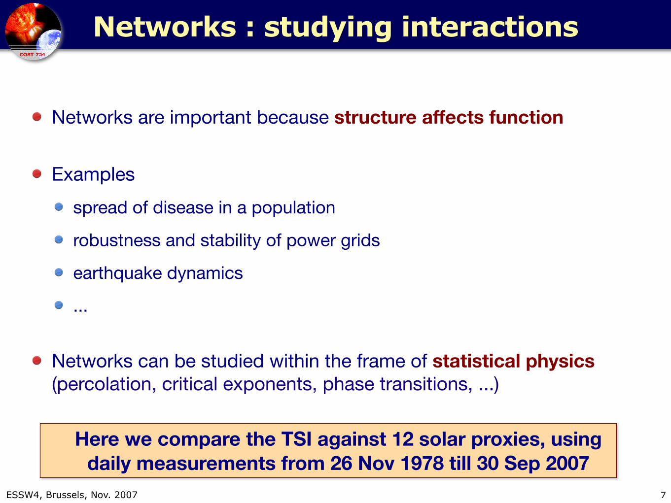
Networks are important because structure affects function

Examples

spread of disease in a population

robustness and stability of power grids

earthquake dynamics

...

Networks can be studied within the frame of statistical physics (percolation, critical exponents, phase transitions, ...)

7


Networks : studying interactions

Networks are important because structure affects function

Examples

spread of disease in a population

robustness and stability of power grids

earthquake dynamics

...

Networks can be studied within the frame of statistical physics (percolation, critical exponents, phase transitions, ...)

7

Here we compare the TSI against 12 solar proxies, using daily measurements from 26 Nov 1978 till 30 Sep 2007


The data

The 12 proxies for solar activity are:

1. ISN : international sunspot number (from SIDC)

2. f10.7 : solar radio flux at 10.7 cm (Penticton Obs.)

3. MgII index : core to wing ratio of Mg II line (R. Viereck, NOAA) —> upper photosphere and chromosphere

4. CaK index : Ca K II equivalent width (Kitt Peak Obs.) —> plages and faculae

5. HeI index : equivalent width of He I line (Kitt peak Obs.) —> plages and faculae

6. Lya index : composite Lyman-α irradiance (T. Woods, LASP)—> upper photosphere up to corona

8


The data

7. MPSI : magnetic plage strength index (Mt. Wilson Obs.) —> contribution from regions with 10 < |B| < 100 G

8. MWSI : Mount Wilson sunspot index (Mt. Wilson Obs.) —> contribution from regions with |B| > 100 G

9. DSA : daily sunspot area (Greenwich Obs.)

10. Mean magnetic field of the Sun (Wilcox Obs.)

11. OFI : optical flare index (Ataç and Özgüç) —> intensity x duration of flares

12. Coronal index (Rybansky) —> total energy emitted by the solar corona in the FeXIV line at 530.3 nm

and

TSI : composite total solar irradiance (PMOD composite)9


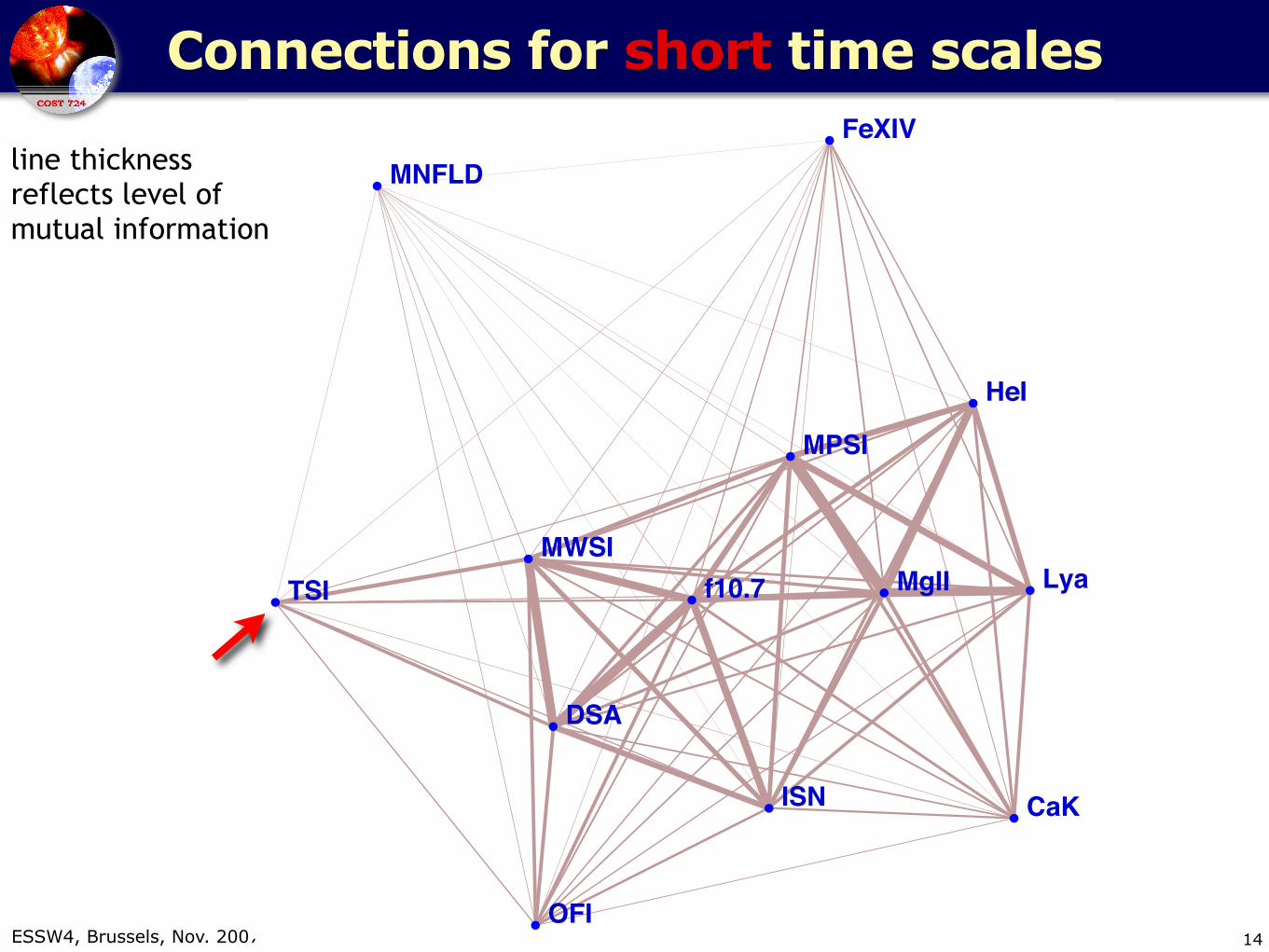
The method

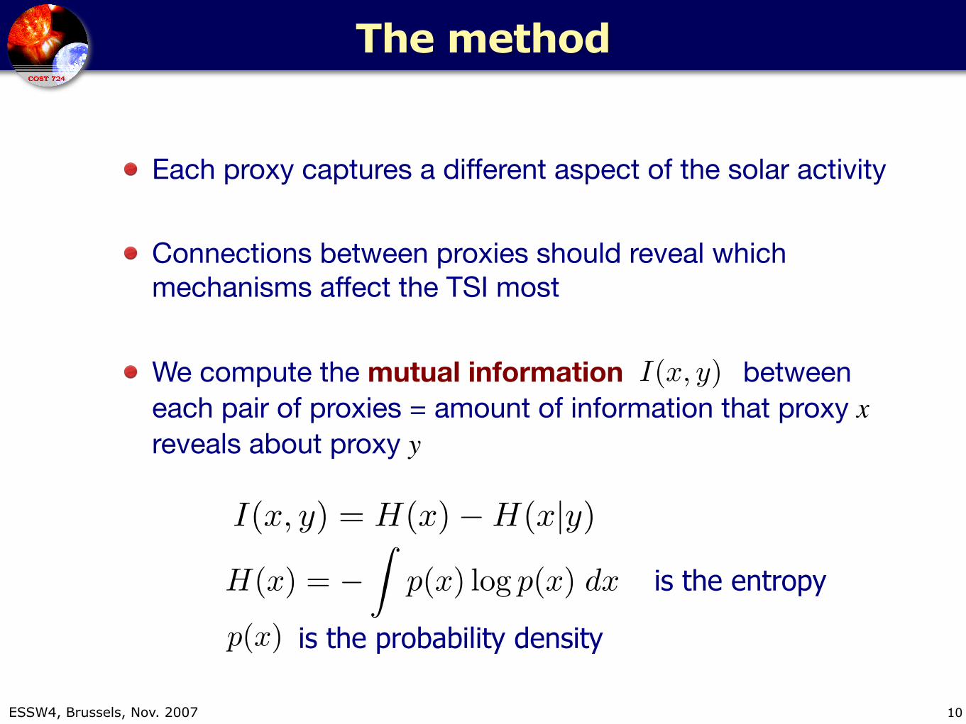
Each proxy captures a different aspect of the solar activity

Connections between proxies should reveal which mechanisms affect the TSI most

We compute the mutual information between each pair of proxies = amount of information that proxy x reveals about proxy y

10

H(x) = !

!p(x) log p(x) dx is the entropy

p(x)

I(x, y)

is the probability density

I(x, y) = H(x) ! H(x|y)


The data

11

0200 ISN

100200300 f10.7

05 MPSI

024

MWSI

0200 MNFLD

05000 DSA

050100 OFI

01020 FeXIV

0.270.280.29

MgII

0.0850.090.0950.10.105

CaK

5060708090

HeI

456 Lya

1975 1980 1985 1990 1995 2000 2005 20101362136413661368

TSI


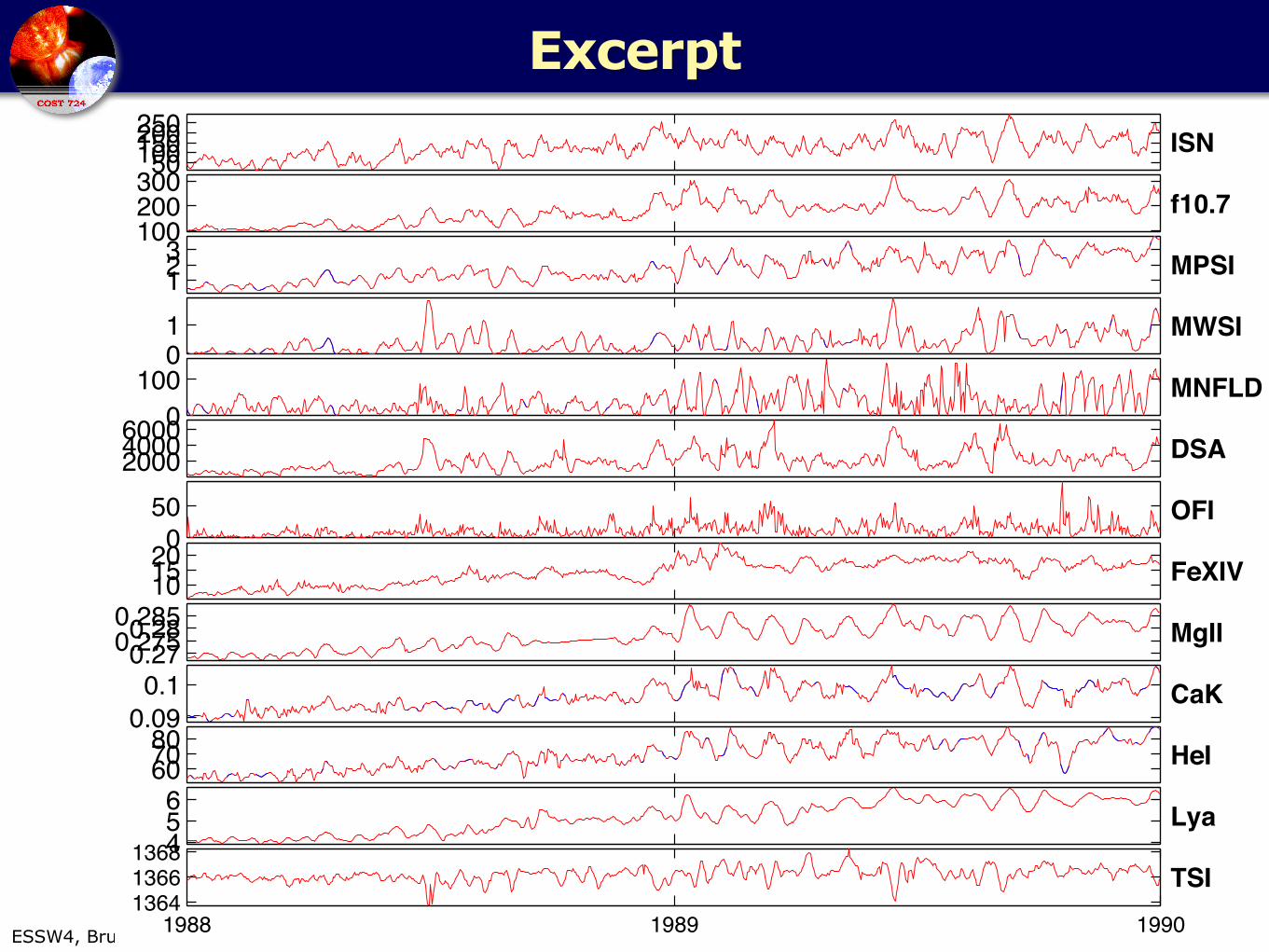
Excerpt

12

50100150200250 ISN

100200300

f10.7

123 MPSI

01 MWSI

0100 MNFLD

200040006000 DSA

050 OFI

101520 FeXIV

0.270.2750.280.285 MgII

0.090.1 CaK

607080 HeI

456 Lya

1988 1989 1990136413661368

TSI


Different scales

The analysis is done separately for

13

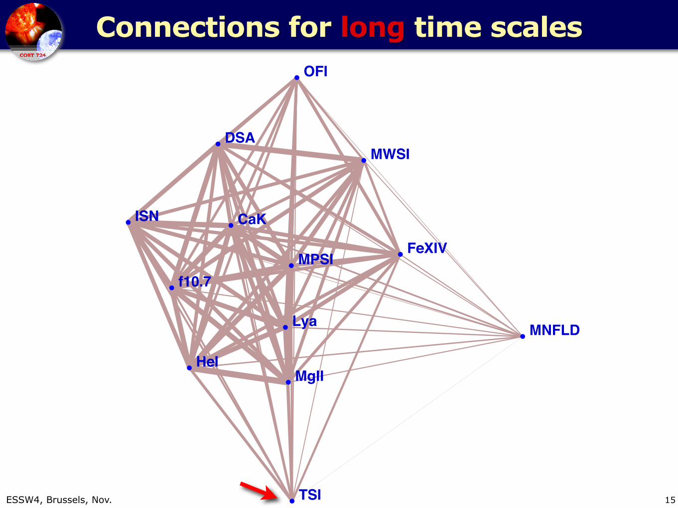
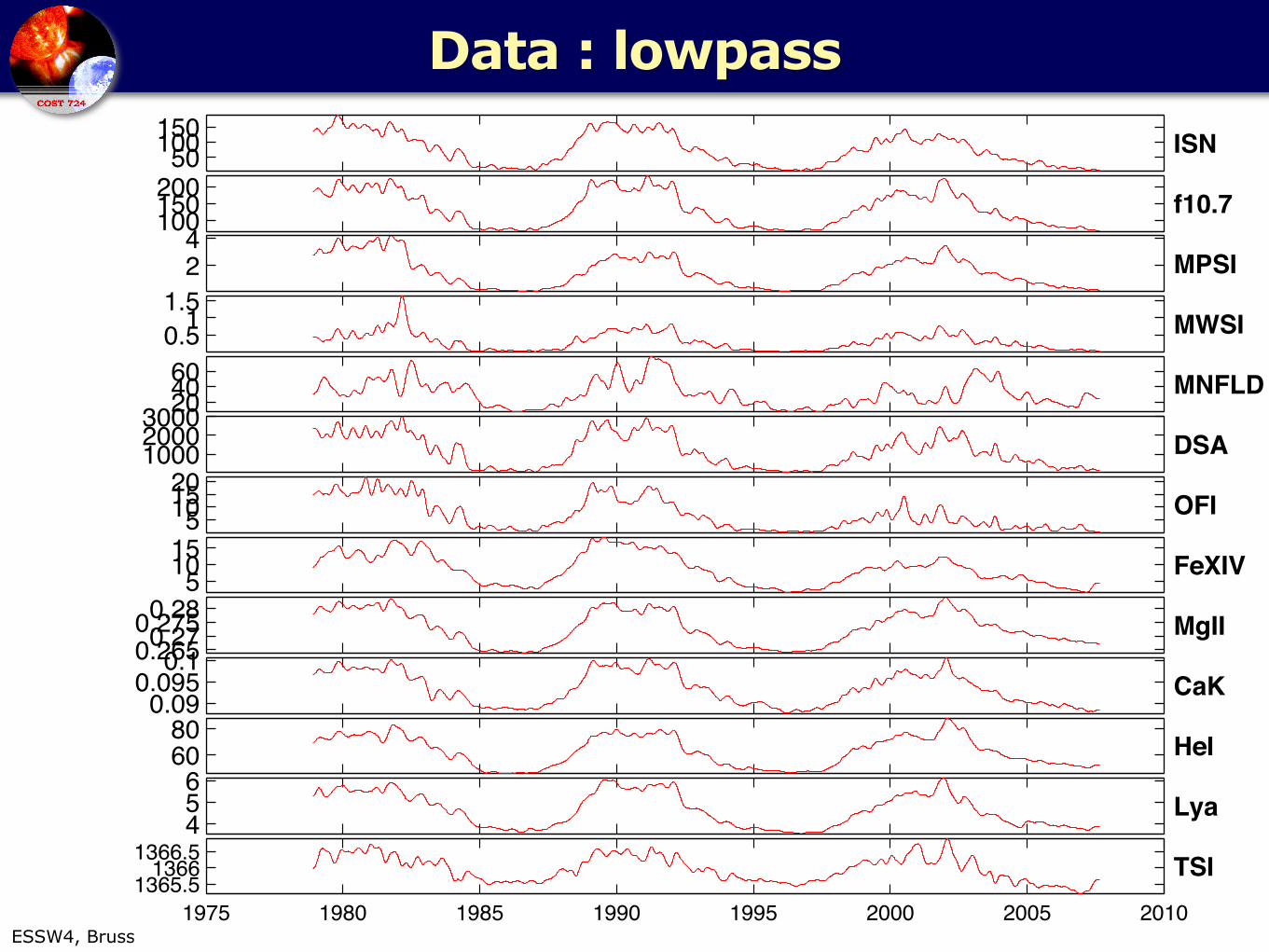
long scale fluctuations> 80 days

effect of solar magnetic cycle + trend

short scale fluctuations< 80 days

effect of solar rotation, center-to-limb effects, ...


ISN

f10.7

MPSI

MWSI

MNFLD

DSA

OFI

FeXIV

MgII

CaK

HeI

Lya TSI

Connections for short time scales

14

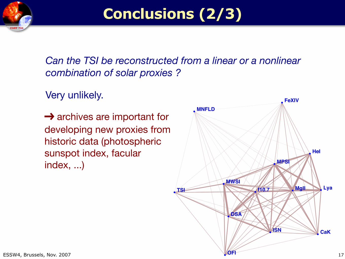
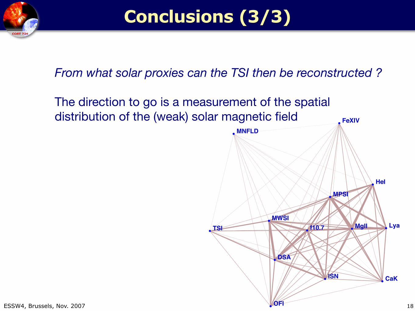
line thickness reflects level of mutual information


ISN

f10.7

MPSI

MWSI

MNFLD

DSA

OFI

FeXIV

MgII

CaK

HeI

Lya TSI

Connections for short time scales

14

Active regions

Plages, faculae, ...

line thickness reflects level of mutual information


ISN

f10.7MPSI

MWSI

MNFLD

DSA

OFI

FeXIV

MgII

CaK

HeI

Lya

TSI

Connections for long time scales

15


ISN

f10.7MPSI

MWSI

MNFLD

DSA

OFI

FeXIV

MgII

CaK

HeI

Lya

TSI

Connections for long time scales

15

Active regions

Plages, faculae, ...


Conclusions (1/3)

16

Which mechanisms contribute to the variability of the TSI ?

for short time scales : regions with intense magnetic fields because they describe the cooling effect of sunspots

for long time scales : ”irradiance” proxies which describe faculae and plages


Conclusions (1/3)

➔ the variability is dominated by the photosphere and the chromosphere

➔ flares do contribute to the variability (poster by M. Kretzschmar)

16

Which mechanisms contribute to the variability of the TSI ?

for short time scales : regions with intense magnetic fields because they describe the cooling effect of sunspots

for long time scales : ”irradiance” proxies which describe faculae and plages


ISN

f10.7

MPSI

MWSI

MNFLD

DSA

OFI

FeXIV

MgII

CaK

HeI

Lya TSI

Conclusions (2/3)

Can the TSI be reconstructed from a linear or a nonlinear combination of solar proxies ?

17


ISN

f10.7

MPSI

MWSI

MNFLD

DSA

OFI

FeXIV

MgII

CaK

HeI

Lya TSI

Conclusions (2/3)


17

Very unlikely.


ISN

f10.7

MPSI

MWSI

MNFLD

DSA

OFI

FeXIV

MgII

CaK

HeI

Lya TSI

Conclusions (2/3)


17

Very unlikely.

➔ archives are important for developing new proxies from historic data (photospheric sunspot index, facular index, ...)


ISN

f10.7

MPSI

MWSI

MNFLD

DSA

OFI

FeXIV

MgII

CaK

HeI

Lya TSI

Conclusions (3/3)

From what solar proxies can the TSI then be reconstructed ?

18


ISN

f10.7

MPSI

MWSI

MNFLD

DSA

OFI

FeXIV

MgII

CaK

HeI

Lya TSI

Conclusions (3/3)


18

The direction to go is a measurement of the spatial distribution of the (weak) solar magnetic field


ISN

f10.7

MPSI

MWSI

MNFLD

DSA

OFI

FeXIV

MgII

CaK

HeI

Lya TSI

Conclusions (3/3)


18

The direction to go is a measurement of the spatial distribution of the (weak) solar magnetic field

➔ include causality: in this coupled system, what causes what ?

19

AB AC

AT AV

AW

BS

BZ

CC

CH

DH

DL

EA

EC

EF

FJ

FS

FZ

GC

HL

HR

IS JL JW

KK

LD

MC

MK ML

MM

MS

PG

PW

RH

RP

RV

TD

WS

YT

Network structure of COST724 team

ESSW4, Brussels, Nov. 2007 20


Data : lowpass

21

50100150 ISN

100150200 f10.7

24

MPSI

0.511.5

MWSI

204060 MNFLD

100020003000DSA

5101520 OFI

51015 FeXIV

0.2650.270.2750.28 MgII

0.090.0950.1

CaK

6080 HeI

456

Lya

1975 1980 1985 1990 1995 2000 2005 20101365.51366

1366.5 TSI

can the total solar days (epoch jan 0, 1980) - sidc.be 4 meteo/dudokdewit_tsi.pdf · can the total...

Documents