Can State and Local Revenue and Expenditure Enhance

Economic Growth? A Cross-State Panel Study of Fiscal Activity

Christopher Arthur Clarke Washington State University

Stephen M. Miller University of Nevada, Las Vegas University of Connecticut

Working Paper 2014-25

September 2014

365 Fairfield Way, Unit 1063

Storrs, CT 06269-1063

Phone: (860) 486-3022

Fax: (860) 486-4463

http://www.econ.uconn.edu/

This working paper is indexed on RePEc, http://repec.org

1

Can State and Local Revenue and Expenditure Enhance Economic Growth?

A Cross-State Panel Study of Fiscal Activity*

Christopher Arthur Clarke Washington State University

Pullman, Washington 99164-4741 christopher.clarke@email.wsu.edu

and

Stephen M. Miller**

University of Nevada, Las Vegas Las Vegas, Nevada 89154-6005

stephen.miller@unlv.edu Abstract The slow economic recovery since the 2008 financial crisis and Great Recession requires state and local governments to continue to make difficult decisions concerning which taxes to raise and which expenditures to decrease in order to maintain a balanced budget. As expenditures usually raise economic growth and taxes generally hinder it, seeking the optimum combination of taxes and expenditures encourages prosperity in a state. In this paper, we study the effects of various expenditures and revenue combinations on growth in real state personal income per capita, using a sample of annual observations from 1977 to 2010 for 49 states and the District of Columbia. We find that state and local governments overfund education and parks, recreation, and natural resources while they underfund hospitals and health spending, once netted for charges and user fees. State and local governments also underutilize corporate income taxes as a source of revenue. Finally, we also estimate non-linear and short- and long-run specifications, which generally support prior findings. JEL: E62, H21, H70, O40, R11 Key Words: Regional growth, state and local finance * The Lee Business School provided a summer grant that supported the research of both

authors. The funding for the first author facilitated the completion his thesis for an MA degree.

** corresponding author

2

1. Introduction

The slow economic recovery since the 2008 financial crisis and Great Recession requires state

and local governments to continue to make difficult decisions concerning which taxes to raise

and which expenditures to decrease in order to maintain a balanced budget. Taxation divorces

the price the seller receives from the price the buyer pays and, thus, causes distortions in market

activity and dead-weight losses in the economy. At the same time, the private economy

underprovides public goods. Higher taxes provide a higher level of public expenditure, which

may foster economic growth. This study considers how the fiscal decisions as to the types of

taxes and expenditures at the state and local level can encourage prosperity in a state.1

This paper analyzes the relationship between fiscal structures, including specific taxes

and specific spending categories, and growth in real per capita personal income, using annual

data from 1977 to 2010. We investigate the effects of specific taxes and specific expenditures on

state and local growth, adding to the literature by considering more disaggregation in the fiscal

variables and by including data from the most recent fiscal crisis and Great Recession. The

inclusion of all sources of revenue, expenditure, as well as the state and local government

surplus, implies that perfect multicollinearity occurs. Thus, we must exclude one of the sources

of revenue, expenditure, or the surplus to estimate our models. We then can interpret the

coefficients as the effect on the growth rate of the economy from an increase in the independent

variable caused by an appropriate offset of the omitted variable. For example, we can compare

the effect of raising corporate taxes or lowering the surplus to fund higher education spending,

and so on. We then do this, in turn, for all offset fiscal variables. Then we can answer the

question of which fiscal revenues and expenditures the state and local government over- or 1 Although this paper investigates how fiscal structure affects economic growth, other factors affect fiscal policy decisions besides enhancing economic growth. For example, the state and local governments provide public goods at the level that the public desires, which need not enhance growth.

3

under-uses for the average state.

We also estimate the short- and long-run effects, adopting the specification of Reed

(2008). Using five-year intervals, we estimate a specification that includes both differenced

variables (i.e., short-run effects) as well as lagged variables (i.e.., long-run effects). His

specification brings added benefits of reducing measurement error and serial correlation.

Finally, Bania, Gray, and Stone (2007) note that focusing on linear incremental effects

does not allow for decreasing returns to expenditure increases. That is, when an expenditure

category (e.g., higher education) first increases, it provides additional public goods or services,

probably enhancing economic growth. Once government sufficiently provides the privately

under-provided public good or service, additional government expenditure will crowd out the

private economy, and therefore reduce growth. We incorporate squared fiscal variables into our

linear specification to estimate the possibility of these “growth hills.”

We find that, on average, reducing state and local government revenue and expenditure

enhances growth. Governments overfund education and transportation while they underfund

police, fire and corrections; utilities, once netted for charges and user fees; and welfare,

unemployment, housing, and community spending. When estimating the long-run effect, we

discover more evidence that additional government spending diminishes growth. Furthermore,

we observe that state and local government underutilizes corporate income taxes as a source of

revenue. We find evidence in support of growth hills, estimating the "optimal level" of growth-

enhancing government revenue to fall between 18 and 30 percent of the economy. Unproductive

government expenditure does not enhance economic growth at any point.

The paper proceeds as follows. Section 2 discusses the relevant literature. Section 3

develops a theoretical framework that generates the specification to estimate the relationship

4

between tax and spending categories and the growth rate of state income. Section 4 discusses the

data and estimation methodology. Section 5 reports and discusses the estimated results. Section 6

concludes.

2. Overview of Previous Research

The literature offers few conclusions as to the effects of taxes on economic growth. Most

conclude that taxes used to fund transfer payments exert small, negative effects on economic

activity. If used for productive purposes, oft times tax increases increase economic growth:

Helms (1985); Phillips and Goss (1995); Miller and Russek (1997), Wasylenko (1997), and

Bania, Gray, and Stone (2007). Other studies, however, show a negative effect on growth:

Mullen and Williams (1994); Besci (1996); and Reed (2008). Even other studies show a weak

effect of taxes on growth: Romans and Subrahmanyan (1979); Wasylenko and McGuire 1985);

Stokey and Rebelo (1995); Lucas Jr. (1990); and Tomljanovich (2004). Most studies focus on the

overall tax burden, they do not study in great detail separate taxes and spending categories.

Helms (1985) recognized the problem of interpreting the coefficient of fiscal variables,

given the government budget constraint. That is, spending must equal revenues plus deficit. This

allows him to separate the effect of overall taxation and expenditure into subcategories. Without

including multiple expenditure options, researchers must interpret the effects on growth as the

effect of raising a tax to finance average expenditures. Helm’s approach allows the analysis of

the different effects from raising a tax to finance, for example, transfer payments or education.

Helms uses the natural logarithm of real state personal income as the dependent variable. The

explanatory variables include both government revenue and expenditure. The revenue

components include property taxes, other taxes, user fees, and federal source revenues. The

expenditure components include health, highways, local schools, higher education, and other

5

expenditures. To avoid perfect multicollinearity, Helms omits transfer payments. He finds, for

example, positive effects from raising public service expenditure financed by lowering transfer

payments, and negative effects of raising taxes to increase transfer payments.

Mofidi and Stone (1990) study the effects of fiscal revenue and expenditure on

investment and employment. Like Helms, they omit transfer payments and find that transfers

exhibit a negative effect. Expenditures on health, education, and infrastructure exert positive

effects. Expanding the decomposition of fiscal variables even further, Miller and Russek (1997),

using fixed effects, investigate the effects of tax and expenditure components on state real GDP

growth GDP from 1978 to 1992. They find that government overuses sales taxes and underuses

corporate income taxes. They also report negative relationships between growth and education,

transportation, and public safety.

Stokey and Rebelo (1995) show that under most circumstances, a consumption tax does

not affect the return on capital and, thus, does not affect investment, output, and productivity.

They also discover that higher property taxes lower the return on reproducible physical capital

and on non-reproducible land. Therefore, increases in property tax rates that lower the return on

capital will reduce growth.

Kneller, Bleaney, and Gemmell (1999) distinguish between distortionary taxes defined as

taxes on income and property, and non-distortionary taxes defined a consumption taxes. They

conclude that while the former reduces growth, the latter does not. Additionally, they find that

productive government spending benefits growth. Similarly, Gemmell, Kneller, and Sanz (2006)

use annual data and include short-run dynamics and confirm the findings of Kneller, Bleaney,

and Gemmell (1999).

Widmalm (2001) discovers that the proportion of tax revenues raised from taxing

6

personal income negatively correlates with growth. Moreover, she documents a tendency for

consumption taxes to enhance growth.

Brown, Hayes, and Taylor (2003) study the effects of taxes and expenditures for state and

local governments across states for the years 1977 to 1997. Using a one-year lag structure for the

fiscal variables, they find that state and local governments underutilize corporate taxes and over

utilize sales and property taxes. They also find welfare spending to enhance growth if funded by

corporate income taxes, but to diminish growth if funded by sales taxes. They also report that

state and local governments overfund both elementary and higher education. Additionally, health

and hospital spending diminish growth in state GDP, if funded by sales or property taxes.

Transportation and housing both grow the economy, if income taxes fund them.

Yamarik (2000), using pooled OLS to estimate the effects of taxes on gross state product

(GSP) from 1977 to 1995, reports that the average tax rate significantly, negatively affects the

growth of GSP. Specifically he concludes that marginal personal income and average property

taxes exhibit a negative relationship with growth. In a later paper, Ojede and Yamarik (2012)

estimate long- and short-run relationships, using the pooled mean-group estimators, leaving out

welfare expenditure. Their short-run findings include a negative effect on growth when increases

in expenditures or property taxes are financed by a reduction in welfare payments. Raising the

deficit to pay for welfare expenditures exhibits a positive effect on growth. In the long run, state

and local expenditures generate a positive effect on growth, if raised by lowering welfare

payments. Deficit, sales tax, and property tax financing of welfare payments all exhibit a

negative effect on growth.

Recently, Reed (2008), in a thorough and robust study, examines growth across states

from 1970 to 1999. Using five-year differences, he consistently finds a negative effect of the tax

7

burden on state economic growth. He estimates under different time periods, different

geographical regions, and various estimation techniques. In imitating Helm’s style, but contrary

to his findings, Reed discovers that raising total taxes to fund non-welfare expenditure exerts a

negative effect on growth both in the long and short run. Reed did not, however, distinguish

between the types of taxes, or the types of non-welfare spending.

3. Theoretical Model

We adapt the Bania, Gray, and Stone (2007) and Bleaney, Gemmell, and Kneller (2001)

presentation of the public-policy endogenous growth model from Barro and Sala-i-Martin

(1992b). In the model, fiscal policy can determine both the level of the output path and the

steady-state growth rate. This differs from the neoclassical growth model, which only allows for

fiscal policy to affect the level of the output path. The production process involves, n producers,

each producing output, y. That is,

𝑦 = 𝐴𝑘1−𝛼[∑ 𝑔𝑖𝑘𝑖=1 ]𝛼, (1)

where A is a positive constant, k is private capital and ( )1,...,ig i k = is a group of publicly

provided inputs, and α is a parameter between zero and one. State and local government funds its

budget with a proportional tax on output at the rate ( )1,...,h h lτ = , a group of tax rates (sales,

property, income, other). This leads to the following state and local government budget

constraint:

𝑛∑ 𝑔𝑖𝑘𝑖=1 + ∑ 𝐶𝑗𝑚

𝑗=1 + 𝑏 = 𝑛𝑦∑ 𝜏ℎ𝑙ℎ=1 , (2)

where ( )1,...,jC j m= is a group of government-provided consumption (or “non-productive”)

goods and b is the budget surplus. The representative, infinite-lived household's utility function

is given as follows:

8

𝑈 = ∫ ((𝑐1−𝜃 − 1) (1 − 𝜃)⁄ )𝑒−𝜌𝑡∞0 𝑑𝑡, 𝜃 > 0, (3)

where -θ is the marginal utility's constant elasticity, c is consumption per person, and ρ>0 is the

constant rate of time preference. Households hold real assets, a(t), with a real rate of return

denoted by r(t). The household’s budget constraint determines saving (i.e., da/dt) or income

minus consumption as follows:

𝑑𝑎 𝑑𝑡⁄ = 𝑟𝑎 − 𝑐. (4)

The first-order condition for maximizing utility subject to the budget constraint requires the

following real rate of return:

𝑟 = 𝜌 + 𝜃 ∙ 𝜅𝑐, (5)

where 𝜅𝑐 is the growth rate of consumption per person.

Firms seek to maximize net revenues. Barro and Sala-i-Martin (1992b) show the first-

order optimization condition includes the relationship

𝑟 = (1 − ∑ 𝜏𝑖𝑘𝑖=1 )(𝑑𝑦 𝑑𝑘)/𝜂⁄ , (6)

where 𝑑𝑦 𝑑𝑘⁄ is the marginal product of capital and η is the constant cost of capital.

We calculate the constant growth rate of per capita consumption by combining equations

(5) and (6) to give

𝜅𝑐 = [�1 − ∑ 𝜏𝑖𝑘𝑖=1 �(𝑑𝑦 𝑑𝑘)⁄ /𝜂 − 𝜌]/𝜃. (7)

The growth rate of c equals the growth rate of y as long as the appropriate transversality

conditions hold. Equation (1) determines the marginal product of capital as follows:

𝑑𝑦 𝑑𝑘⁄ = (1 − 𝛼)𝐴�[∑ 𝑔𝑖𝑘𝑖=1 ] 𝑘⁄ �

𝛼, (8)

which transforms into

𝑑𝑦 𝑑𝑘⁄ = (1 − 𝛼)𝐴(1−𝛼)(1−𝛼)[∑ 𝑔𝑖𝑘

𝑖=1 ]𝛼(1−𝛼)(1−𝛼) 𝑘−𝛼. (9)

Eventually, the equation reduces to

9

𝑑𝑦 𝑑𝑘⁄ = (1 − 𝛼)𝐴1

1−𝛼([∑ 𝑔𝑖𝑘𝑖=1 ] 𝑦⁄ )

𝛼1−𝛼. (10)

Finally, plugging this result into equation (7), we determine the growth rate of the

economy, V, as follows:

𝑉 = 𝑤�1 − ∑ 𝜏ℎ𝑙ℎ=1 �(1 − 𝛼)𝐴1 (1−𝛼)⁄ �[∑ 𝑔𝑖𝑘

𝑖=1 ] 𝑦⁄ �𝛼 (1−𝛼)⁄

− 𝑚, (11)

where 𝑤 = 1 𝜃⁄ and 𝑚 = 𝜌/𝜃. The model determines private capital endogenously and,

therefore, private capital does not appear in equation (11). Output growth in the steady state

depends only on structural parameters for production and utility (w, m, α, and A), the tax rates (

hτ ) and the ratio of productive government expenditures to output, (�∑ 𝑔𝑖𝑘𝑖=1 �/𝑦).

For empirical testing, suppose that the growth rate, 𝑉𝑠𝑡, at time t in state s depends on the

fiscal variables from equation (2), 𝑋𝑖𝑠𝑡, state fixed effects (which control for time-invariant

characteristics such as geography, natural amenities, distance from markets, and time-invariant

government regulation), 𝜑𝑠, time fixed effects (which control for macroeconomic forces and

federal government activity), 𝛾𝑡, and three state control variables – lagged real per capita

personal income, 1sty − , the population growth rate, stn , and the unemployment rate, 𝑢𝑠𝑡. That is,

𝑉𝑠𝑡 = 𝛽0 + 𝛽1𝑦𝑠𝑡−1 + ∑ Β𝑖𝑋𝑖𝑠𝑡𝑘𝑖=1 + 𝛽2𝑛𝑠𝑡 + 𝛽3𝑢𝑠𝑡 + 𝜑𝑠 + 𝛾𝑡 + 𝜔𝑠𝑡, (12)

where 𝛽0, 𝛽1, 𝛽2, 𝛽3, and the vector Β𝑖 are parameters to be estimated. In practice, this equation

is similar to the reduced form equation found in Miller and Russek (1997) and Brown, et al.

(2003).

The linear budget constraint in (2) indicates that

𝑋𝑘𝑠𝑡 = −∑ 𝑋𝑖𝑠𝑡𝑘−1𝑖=1 . (13)

Hence, we must omit one fiscal variable to prevent perfect multicollinearity. Equation (12) then

becomes,

10

𝑉𝑠𝑡 = 𝛽0 + 𝛽1𝑦𝑠𝑡−1 + ∑ (Β𝑖 − Β𝑘)𝑋𝑖𝑠𝑡𝑘−1𝑖=1

+𝛽2𝑛𝑠𝑡 + 𝛽3𝑢𝑠𝑡 + 𝜑𝑠 + 𝛾𝑡 + 𝜔𝑠𝑡. (14)

That is, the fiscal coefficients measure the effect of a unit change in the variable offset by the

corresponding change in the omitted variable from the regression. For example, if we omit

corporate income taxes, then the coefficient for welfare, unemployment, and housing measure

the expected increase in the growth rate due to a one unit increase in welfare, unemployment,

and housing spending funded by an increase in the corporate income tax.

4. Data

Personal income for each state and the District of Columbia, population, and fiscal variables for

each state come from U.S. Department of Commerce, Bureau of the Census’ Government

Finances database. Unemployment rates for each state come from the U.S. Department of Labor,

Bureau of Labor Statistics. We compute real per capita personal income using the national GDP

deflator, since a consistent state level price index does not exist over our sample period.

The Census did not collect data for local finances and consequently state and local

finances for the years 2001 and 2003. It did, however, collect state data for these two years.

Using these data, we interpolate the state and local fiscal variables by estimating the following

equation,

𝑆&𝐿𝑠𝑡 = 𝜎0 + 𝜎1𝑆𝑡𝑎𝑡𝑒𝑠𝑡 + 𝜎2𝑢𝑠𝑡 + 𝜎3𝑡 + 𝜎4𝑡2 + 𝜑𝑠 + 𝑒𝑠𝑡. (15)

where & stS L denotes a state and local fiscal variable, stState denotes the comparable state fiscal

variable, stu is the unemployment rate, t is time, sϕ are state fixed-effects, ste is the error term,

and the elements of the vector σ are parameters to be estimated. We then include the predicted

11

values of for the & stS L variables for the years 2001 and 2003 in the original series.2

We approximate the dependent variable as 𝑉𝑠𝑡 = ln(𝑦𝑠𝑡) − ln(𝑦𝑠𝑡−1), where sty is real

per capita personal income. The use of a per capita measure of output matches the work of Miller

and Russek (1997), Yamarik (2000), Bleaney, Gemmell, and Kneller (2001), Bania, Gray and

Stone (2007), and Reed (2008). Dividing personal income by population allows the coefficients

to measure the effect of differences in growth over and above population increases, and real

personal income per capita measures the standard of living or quality of life.

We examine the fiscal variables both at the aggregate and disaggregated levels. The

aggregate variables include total revenue, total expenditure, net intergovernmental revenue

(intergovernmental revenue minus intergovernmental expenditure), and surplus. Net

intergovernmental revenue captures the net federal taxes brought back to the state. The

disaggregated revenue variables include property taxes, sales taxes (which includes sale of

property, but excludes the public utility sales tax), individual income tax, corporate income tax,

and other revenues. The expenditure variables include police, fire, and correction facilities;

transportation; higher education; secondary education; hospitals and health; parks, recreation,

and natural resources; welfare, housing and community, and unemployment expenditures; and

other expenditures. Finally, we also include net utility expenditures.3 Government Finance

categorizes public transit spending in the total utilities. We move these expenditures to the

transportation section. We also include solid waste and sewerage services, which are self-

classified, in total utilities expenditure.

Because we address the issue of the effects of tax distortion, we net out revenue charges

2 We conduct the regression using level variables rather than natural logarithms because a few of the variables include negative values 3 Positive net expenditure on utilities occurs for 65% of the observations.

12

and fees. For example, parks and recreation charges include revenues gathered from the use of

facilities operated by the government (swimming pools, community recreation centers,

museums, and so on) (see the U.S. Bureau of the Census 2006). These revenue streams are not

distortionary.4 Therefore, in evaluating the effect of tax revenue to supply public services, we

remove the corresponding charges from the expenditure. Different revenue sources cover the

remaining portion of the expenditure not financed by charges and fees. The charges and fees

recorded by the Census include air transportation, highways, water transportation, parking,

education, hospital, parks and recreation, natural resources, housing and community, and other

charges. In addition, we subtract utility revenues and liquor store revenues from their respective

expenditures. Brown, Hayes, and Taylor (2003) incorporate net utilities and subtract tuition from

education, but they do not do this for all applicable variables. They also include total charges and

tuition as separate revenue variables. This specification allows tuition to fund other expenditures.

In reality, if the state did not provide education, it would not collect tuition revenue. Our

approach of netting charges from expenditure provides a differentiation from the existing

literature. The Appendix provides more information on fiscal variable series.

We divide the fiscal variables by state personal income and multiply by 100, giving an

"effective average tax rates” in a state (Helms, 1985). Table 1 reports descriptive statistics for

each variable.

The growth rate averaged 1.94%, ranging from -14.54% (Wyoming in 2009) to 17.64%

(North Dakota in 1981). The unemployment rate averaged 6.61%. Total revenue averaged

18.23% of state personal income. Tennessee experienced the minimum (10.08% in 2009) and

Wyoming experienced the maximum (43.62% in 2001). Total expenditure ranges from 10.71%

4 Here, we must assume that the charge or fee equals the marginal cost of providing the good or service.

13

(North Dakota in 1985) to 32.38% (D.C. in 1977), averaging 17.46%. Sales taxes provide the

largest source of revenue (3.54%) with property taxes a close second (3.11%). Secondary

education receives the largest spending (4.27%). Welfare, unemployment compensation, and

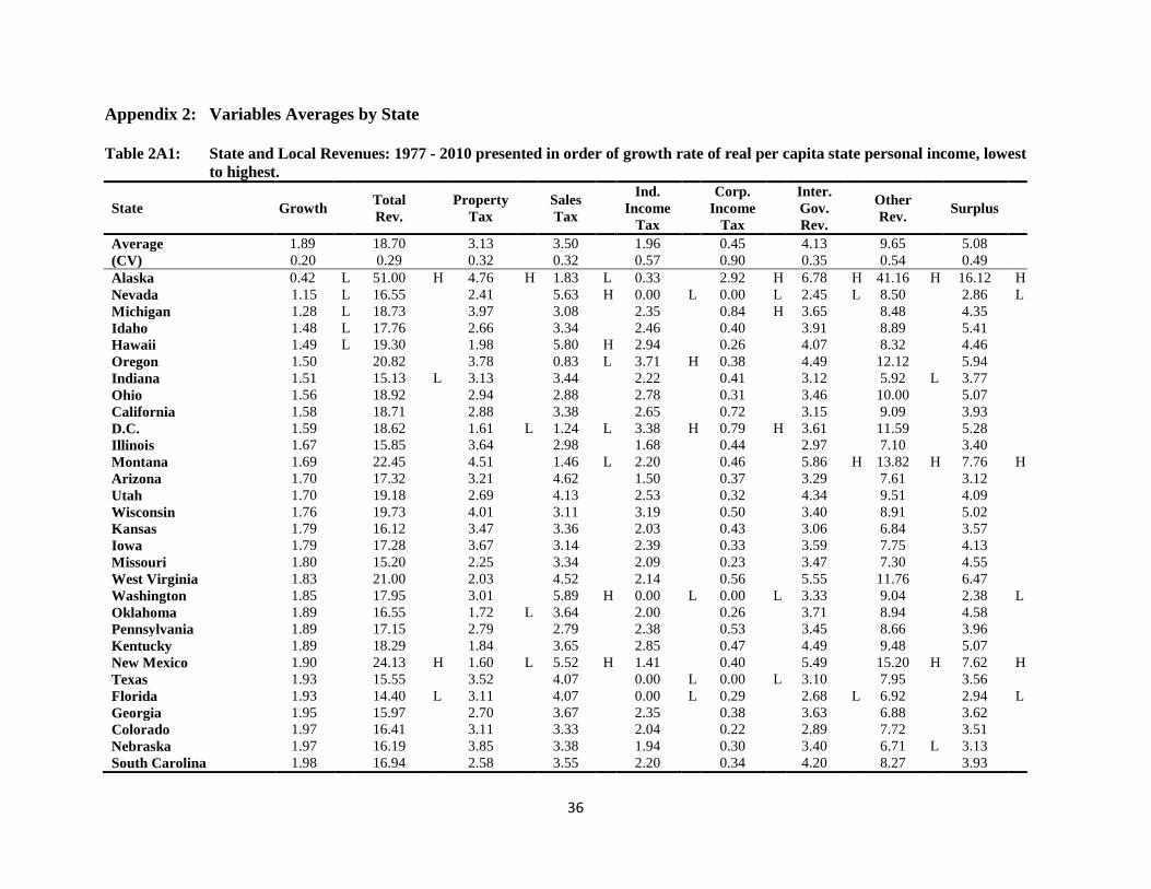
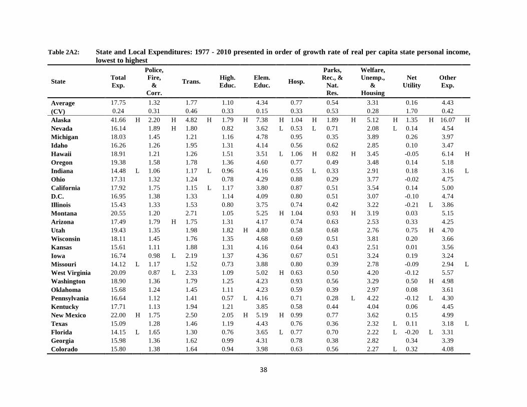
housing and community expenditure comes in second (3.36%). Table A1 and A2 report the

means by state for revenue and expenditure, respectively.

Pre- and post-financial crisis

The Great Recession began with the financial crisis in the autumn of 2008. Table 2 reports the

difference in government fiscal activity from before and after the crisis. The Census

Classification Manual defines a year as follows: “each individual government fiscal year that

ended between July 1 of the previous year and June 30 of the survey year.” Table 2 lists the

average descriptive statistics for 2007 and 2008 as well as 2009 and 2010.

The mean growth rate of real per capita personal income completely reverses from 2.05%

to -2.30%. The unemployment rate doubles from 4.93% to 8.84%. Revenues decrease from

19.41% of personal income to 16.30%. At the same time, expenditures increase from 18.38% to

20.60%. This results in the surplus dropping from 5.48% of state personal income to just 1.11%.

Interestingly, for a recession starting with the bursting of a housing bubble, property taxes rise

from 3.09% to 3.41%, indicating that total property tax revenue fell less than state personal

income. Sales taxes remain mostly unchanged, while the income taxes decrease modestly.

On the expenditure side, net utilities remain constant as a share of personal income.

Police, fire, and correction facilities; transportation; education; and parks, recreation, and natural

resources increase modestly. Health and hospital decrease 76% from a share of 0.84% to 0.20%.

Welfare, unemployment compensation, and housing and community spending increase

dramatically from 3.98% to 5.04%.

14

Estimation

The theoretical model suggests that some revenues and expenditures are distortionary while

others are not. Rather than judging a priori the nature of each variable, we omit each variable, in

turn. Because of collinearity, each of these regressions is, in essence, the same regression.

The study covers 1977 to 2010 over 49 states5 and the District of Columbia, implying

1700 observations in the panel data set. The data for the personal income includes 1976. Because

the personal income data run over the calendar year, and the budget data run over the fiscal year,

an implied six month lag exists in the regressions. We estimate each specification using the two-

way fixed-effect model with robust panel-corrected standard errors. First, we estimate the

equation including aggregated fiscal variables to test the level of overall expenditure and

revenue. Next, we estimate the equation with disaggregated fiscal variables. Then, we estimate

the specification that captures short- and long-run effects using aggregated and disaggregated

fiscal variables. Lastly, we estimate the specification with growth hills using only aggregated

fiscal variables.

The specification for growth hills is as follows:

𝑉𝑠𝑡 = 𝛽0 + 𝛽1𝑦𝑠𝑡−1 + ∑ (𝐵𝑖𝑋𝑖𝑠𝑡 + 𝑆𝑖𝑋𝑖𝑠𝑡2 )𝑘𝑖=1

+𝛽2𝑛𝑠𝑡 + 𝛽3𝑢𝑠𝑡 + 𝜑𝑠 + 𝛾𝑡 + 𝜔𝑠𝑡. (16)

Once again, we leave out each fiscal variable, in turn, for each regression. Since the squared

terms of net intergovernmental revenue and surplus are insignificant and the point estimate close

to zero, we omit them in the regression.

5. Results

Table 3 presents the results from the aggregated estimation. Two of the three state control

5 We omit Alaska due to the extreme nature of their government’s fiscal behavior, most of which reflects the pipeline built in 1977.

15

variables exert significant effects. First, the lagged real personal income per capita produces a

significant negative effect on the growth rate of real personal income per capita at the 1-percent

level. This result conforms to the β-convergence hypothesis at the state and local level (e.g., see

Barro and Sala-i-Martin 1992a). Second, the unemployment rate causes a significant negative

effect on the growth rate at the 1-percent level, the expected finding. For each additional

percentage rise in the unemployment rate, growth is expected to slow by -0.30%. Finally, the

population growth rate, although negative, does not generate a significant effect on the growth

rate.

Higher total revenue and higher total expenditure generally generate significant negative

effects on the growth rate. The exception occurs when revenue is raised to increase the surplus.

This particular fiscal action causes a significant increase in the growth rate. This indicates that

state and local governments raise too much revenue and spend too much, on average. From

theory, this would indicate that the average state spends too much on unproductive expenditures.

Miller and Russek (1997) suggest another possibility. To wit, total expenditure and total revenue

exhibit less cyclical volatility than personal income, implying that cyclical effects may cause the

negative correlation. Finally, we note that raising the fiscal surplus either by raising revenue or

by reducing spending significantly increases the growth rate. Three additional comments provide

some caution about our findings. First, we only consider the effect of fiscal variables on the

economic growth rate in per capita real personal income, and not the public’s demand for public

good provision. Second, these results only inform us in a broad sense. That is, they do not

provide information on which particular type of government spending diminishes growth. Third,

the current specification focuses on short-run effects of fiscal variables. A latter specification

provides some evidence on both the short- and long-run effects of changes in fiscal structure.

16

The coefficients in Tables 3 as well as in Tables 4, 5, and 6 are symmetric. For example,

in the first column of Table 3, when a state raises total expenditure by one percent of state

personal income, it must do so by raising total revenue and the growth rate of the economy

decreases by -0.33 percent, on average. In the second column, when a state increases revenue by

one percent of state personal income, again, it must do so only by raising total expenditure and

again the growth rate changes by -0.33 percent. These two specifications measure the same event

and yield the same coefficient. When considering two revenue or two expenditure variables, the

coefficients exhibit the same magnitude, but the opposite sign. When considering one revenue

variable and one expenditure variable, the magnitudes of the coefficient remain the same but the

sign remains the same.

Table 4 displays the disaggregated results. Again, two of the three state control variables

exhibit significant effects. As before both the lagged real personal income per capita and the

unemployment rate each exert a significant negative effect on the growth rate and the population

growth rate does not exhibit a significant effect, although, once again, the coefficient is negative.

Transportation and higher education expenditures both exhibit a consistent significant

negative effect on economic growth at the 1-, 5-, or 10-percent levels. For both expenditure

variables, 13 out 15 coefficients possess significant effects on growth in state personal income.

Funding it by any source of revenue uniformly yields a negative effect. No significant effect

emerges when each of these two expenditures provides the funding source for the other

expenditure as well as when the funding source in parks, recreation, and natural resource

expenditure. The negative effect consistently proves higher and/or more significant for higher

education expenditure. For higher education expenditure, the significant decreases on the growth

rate range from a low magnitude of -1.38% (secondary education) to a high magnitude of -2.37%

17

(corporate income tax). The significant coefficients for transportation expenditure all fall around

-1.00%. Secondary education expenditure produces 8 significant negative coefficients as well as

significant positive coefficients, if the funding of secondary education comes from transportation

and/or higher education spending. Increasing spending on parks, recreation, and natural

resources produces negative effects on the growth rate, although the coefficients only

occasionally prove significant at the 10-percent level.

Fiscal spending for net utilities; police, fire, and correction facilities; health and hospitals;

welfare, unemployment, housing, and communities sometimes generate significantly positive

effects on the growth rate. At no time do the estimated coefficients for these spending variables

indicate a significant negative effect. For health and hospitals, the significant positive effects

occur only for reductions in transportation and higher education expenditure. For net utilities;

police, fire, and correction facilities; and welfare, unemployment, housing, and communities

spending, other sources of financing that produce significant positive effects on the growth rate,

in addition to reduced transportation and higher education spending, come from increased

individual income tax revenue, and reduced secondary education and parks, recreation, and

environmental spending.

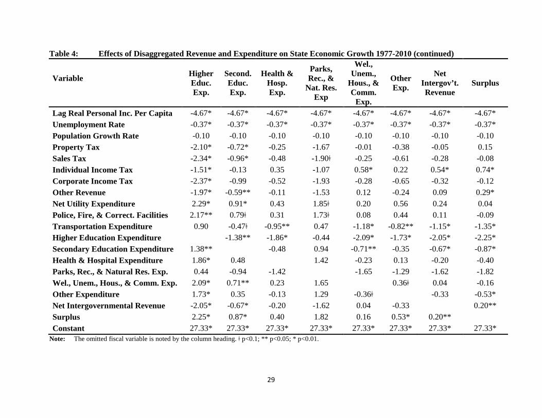
The evidence suggests that states overfund transportation and education for the average

state.6 For education funding, this finding agrees with those of Brown, et al. (2003) and Miller

and Russek (1997), but contradicts those of Mofidi and Stone (1990) and Helms (1985). This

may reflect a lack of correlation between the quality of education and the money spent on

education. Furthermore, Miller and Russek (1997) suggest that it may reflect a disincentive for

states to invest in human capital. “Better to let someone else exhaust resources on education and 6 To test the hypothesis that states “built” too many buildings for education, we also performed the analysis using education minus capital outlays. The coefficients for higher education became slightly less negative, while the coefficients for secondary education became slightly more negative.

18

then hire the improved product away.” Because transportation and education spending may not

affect growth in real personal income per capita in the short run, we consider the short- and long-

run effects of transportation and education spending later in this paper.

Increasing the budget surplus indicates a benefit to growth in state real per capita

personal income. The coefficients for surplus range from 0.20% (net intergovernmental revenue)

to 2.25% (higher education). Increasing the individual income taxes produces significant positive

effects on the growth rate when some other taxes decrease (property, sales, other, and

intergovernmental revenue) as well as when other expenditures increase (net utility and welfare,

unemployment, housing and community spending). An increase in the individual income tax

produces a negative effect on the growth rate for increasing transportation and higher education

spending. Increasing the property or sales tax revenue to finance transportation and higher

education spending also generates a significant negative effect on economic growth.

The evidence suggests that states rely too little on the individual income tax and too

heavily on property and sales taxes.

Long-Run Effects and Measurement Error

Annual data are particularly vulnerable to measurement error bias. Reed and Rogers (2006)

estimate the roughly one-half of the annual variation in tax burden reflects factors other than tax

policy. Evans and Karras (1994) characterize annual state-level income data as containing

substantial serial correlation. To partly address these problems and following Reed (2008), we

use multi-year interval data. Measurement errors more likely cancel over longer time periods and

serial correlation becomes less severe when observations stand further apart in the time

dimension. An additional advantage comes from the fact that the states use different calendar

dates for their fiscal years. Since the state control variables and real personal income per capita

19

use the calendar year, extending the lag back in time ameliorates this timing issue.

In sum, as a further robustness check and to consider longer-term relationships between

revenue, expenditure, and growth, we estimate the regression using 5 year intervals and

incorporating a 5 year lag into the fiscal variables. Consistent with Reed (2008), the data now

include observations for the years 1977-1981, 1982-1986, … , 2002-2006, for 300 observations.

The estimated equation becomes as follows:

𝑉𝑠𝑡 = 𝛽0 + 𝛽1𝑦𝑠𝑡−1 + ∑ [𝐷𝑖(𝑋𝑖𝑠𝑡 − 𝑋𝑖𝑠𝑡−4) + 𝐿𝑖𝑋𝑖𝑠𝑡−4]𝑘𝑖=1

+𝛽2𝑛𝑠𝑡 + 𝛽3𝑢𝑠𝑡 + 𝜑𝑠 + 𝛾𝑡 + 𝜔𝑠𝑡. (16)

Another mathematically equivalent specification of the fiscal variables is

∑ [𝐷𝑖𝑋𝑖𝑠𝑡 + (𝐿𝑖 − 𝐷𝑖)𝑋𝑡−4]𝑘𝑖=1 . (17)

Table 5 reports the results for the aggregate fiscal variables. Lagged real personal income

per capita and the unemployment rate prove significantly negative at the 1-percent level. Now,

however, the population growth rate exerts a significantly negative effect on economic growth at

the 5-percent level.

The estimated coefficients for the fiscal variables continue to tell a similar story as those

found in Table 3. The short-run effects captured by the change in the fiscal variable over the 5-

year interval show the same signs and same significance. The exception is intergovernmental

revenue, which no longer proves significant. as those results reported in Table 3. Moreover, the

coefficients in Table 5 uniformly exceed those in Table 3.

The long-run effects captured by the 5-year lagged levels of the series provide some

significant findings. The positive effect of financing an increase in the fiscal surplus with higher

revenue or lower spending continues in the long run, albeit with smaller coefficients than for the

short run: 0.30 rather than 0.63 for increasing revenue and 0.42 rather than 1.02 for decreasing

20

spending. The short-run significant negative effect of raising revenue by increasing spending or

increasing spending by raising revenue of -0.39% disappears in the long run, That is, the long-

run effect equals -0.12%, but proves insignificant.

Table 6 displays the estimates the long-run effects of disaggregated revenues and

expenditures. Recall that because of perfect multicollinearity, each regression is the same. Since

there are only 300 observations, in contrast to the 1700 observation before, there are less

statistically significant relationships. In general, the coefficients are larger. This could illustrate

the lag in the effect that fiscal activity has on economic growth. It could also reflect correction

for the biases mentioned previously.

The most influential fiscal variables from the analysis displayed in Table 4,

transportation, higher education, and secondary education expenditures, see a largely smaller role

in terms of significant coefficients and a much less influential variable, parks, recreation, and

natural resource expenditure, plays a much more prominent role in terms of significant

coefficients. Consider parks, recreation, and natural resource expenditure. In the long run, 15 of

the 16 coefficients prove significantly negative whereas in the short run, 14 of 16 coefficients

prove significantly negative. Transportation, higher education, and secondary education

expenditures see fewer significantly negative coefficient estimates. The significantly negative

coefficients for higher education generally point to long-run effects whereas for secondary

education generally point to short-run effects. Transportation expenditure does not show a

pattern for long-and short-run coefficients that are significantly negative.

The fiscal surplus shows a pattern in that all significant coefficients are positive,

indicating that growing the surplus leads to economic growth. These effects come in both the

short- and long-run. The individual income tax generally shows positive coefficients when they

21

are significant. Moreover, most of the significant positive coefficients appear in the long-run and

not the short run. The sales tax coefficients when significant are generally negative. Moreover,

the sales tax predominantly exerts its negative effect in the short run and not the long run.

The corporate income tax now exhibits a few significant positive coefficients. These

occur in the short run.

Growth Hills

In an effort to explain the variety of econometric results for the effect of taxation on economic

growth among the literature, Bania, Gray, and Stone (2007) argue that all findings could

accurately reflect outcomes in Barro-style growth models. That is, in such models, taxes can

exert negative, no, or positive effects on growth. The effects rely on the initial level of taxes and

what the tax revenues fund. For relatively low taxes, revenue increases spent on productive

expenditure will exhibit a positive effect on growth. For relatively high taxes, this effect may

turn negative.

The theory differentiates between productive and nonproductive expenditures in their

effect on economic growth. Rather than judging a priori what constitutes productive and

nonproductive expenditures, we incorporate the findings from Tables 4 and 6, defining

nonproductive expenditure as parks, recreation, and natural resources; higher education;

secondary education; welfare, unemployment, and housing and community; and transportation

and defining productive expenditure as hospital; net utility; police, fire, and corrections facilities;

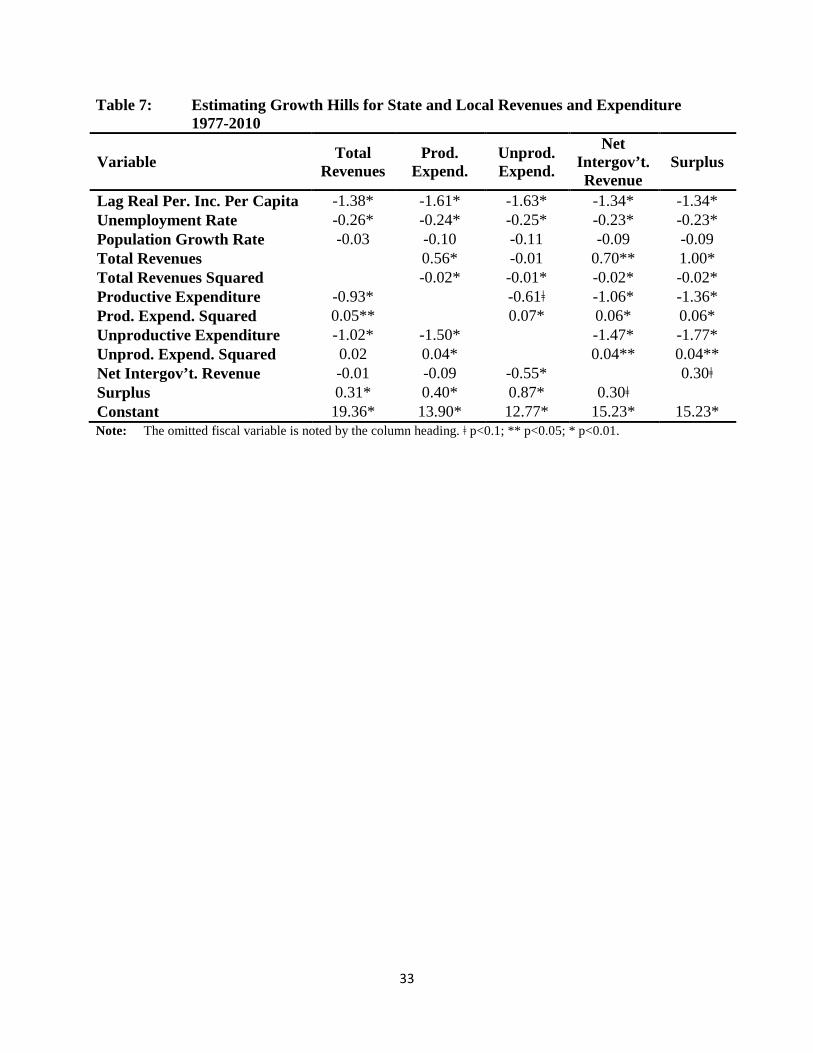
and other expenditures. Table 7 displays the results. From the results, we estimate the peak of a

growth hill for total revenue, where 𝑇𝑜𝑡𝑎𝑙 𝑅𝑒𝑣𝑒𝑛𝑢𝑒 = −𝐵1 2𝑆1⁄ . For the four equations the

estimated growth maximizing share of revenue to personal income are respectively: 17.86, -0.21,

21.29, and 30.30. Revenue that funds nonproductive expenditure diminishes growth at any point

22

for the states in the time period in the sample. Increasing nonproductive expenditures decreases

growth at an increasing rate.. The other three estimates give an estimate as to the ideal revenue to

personal income ratio. The higher point estimate for revenue funding surplus, suggests the

negative effect that state budget deficits impose on the state economy.

6. Conclusion

This paper examines the effect of state and local revenues and expenditures on growth in real per

capita personal income across 49 states and the District of Columbia using a sample from 1977

to 2010. We investigate the issue under the framework of a constant government budget

constraint: revenues equal expenditures plus surplus.

Policy makers consider more goals than simply to grow state personal income. Certain

desirable aspects in policy makers’ objective functions do not reflect the level of real personal

income per capita. Therefore, our findings abstract from other goals besides the growth rate of

real personal income per capita. Readers need to keep this fact in mind when reviewing our

findings.

We find that state and local government collect too much revenue. If revenues increase

by one percent as a share of personal income to finance a similar increase in general expenditure,

the growth rate of the economy shrinks by -0.33%. The same outcome occurs from increasing

general spending by one percent and financing this with the same increase in revenue.

We then disaggregate revenue and spending into subcategories to reinvestigate the

question. In our basic model, we find that transportation, higher education, and secondary

education spending generally reduces economic growth. At the same time, parks, recreation, and

natural resource spending does not exert many significant effects on economic growth, although

the signs and magnitudes of the coefficients seem comparable to the signs and magnitudes of

23

coefficients on transportation, higher education, and secondary education spending. The

coefficients generally prove insignificant in a statistical sense. When we specify the model to

consider both short-run and long-run effects, the results reverse themselves somewhat between

these four variables. Now, parks, recreation, and natural resource spending exhibits many

significantly negative coefficients in both the short and long run. The number of significantly

negative coefficients for transportation, higher education, and secondary education spending

falls, although many significant coefficients still exist. For higher education spending, now the

significantly negative coefficients tend to fall in the long run effects whereas the secondary

education spending possesses significant negative coefficients in the short run. Agreeing with the

later literature Brown, et al. (2003) and Miller and Russek (1997), we find that government

overfunds education spending for the average state.

State and local governments underutilize the corporate income tax. Relying more on a

corporate income tax reduces market distortions caused by property taxes, individual income

taxes, sales taxes, and federal tax sources. Increases in growth occur when some other taxes

decrease (property, sales, other, and intergovernmental revenue) as well as when other

expenditures increase (net utility and welfare, unemployment, housing and community

spending).

Starting at zero, increasing revenue to fund productive expenditure, the surplus, or

replace net intergovernmental revenue increases growth. Eventually, the growth rate starts to

decrease as diminishing returns set in. For spending on these growth enhancing expenditures, we

estimate that the optimal points lie between 17.86 and 30.30. The average level of spending for

the sample falls in this range at 18.23 percent of total state personal income. Yet, recall that this

includes spending on productive as well as unproductive expenditure.

24

Government taxation and expenditure should provide public goods that the private

economy underprovides with minimal tax distortion. As state and local government move from

overprovided expenditures to more underprovided expenditures and implement optimal taxation,

state economies will grow at higher rates.

25

Table 1: Summary Statistics: 1977-2010

Variable Mean Std. Dev. Min Max

Growth Rate of Real Personal Income per Capita 1.94 2.61 -14.54 17.64 Lagged Real Personal Income per Capita 3.29 0.26 2.63 4.18 Unemployment Rate 6.61 2.19 2.30 19.30 Population Growth Rate 1.01 1.08 -5.99 7.32 Total Revenue 18.23 3.56 10.08 43.62 Total Expenditure 17.46 3.16 10.71 32.38 Net Intergovernmental Revenue 4.08 1.64 1.77 17.86 Surplus 4.86 2.74 -3.43 28.70 Property Tax 3.11 1.10 0.97 8.42 Sales Tax 3.54 1.14 0.70 7.47 Individual Income Tax 2.03 1.15 0.00 4.93 Corporate Income Tax 0.41 0.24 0.00 1.36 Other Revenue 9.15 3.09 1.84 36.08 Net Utility Expenditure 0.13 0.42 -0.64 5.50 Police, Fire, & Correction Facilities 1.34 0.45 0.62 4.92 Transportation 1.78 0.79 -0.64 11.07 Higher Education 1.08 0.38 0.16 2.74 Secondary Education 4.27 0.69 2.56 8.65 Health & Hospital 0.79 0.33 -0.21 2.78 Parks, Recreation, & Natural Resources 0.51 0.23 0.13 1.70 Welfare, Unemployment, Housing & Community 3.36 1.23 0.94 8.82 Other Expenditure 4.20 1.10 1.58 9.57

Note: Appendix 1 provides the description of the fiscal variables. We deflate all fiscal variables by personal income and multiply the result by 100. We also express growth rates as percentages. Finally, we take the natural logarithm of lagged real personal income per capita.

26

Table 2: Summary Statistics: Before and After Start of Great Recession

Variable 2007-2008 2009-2010

Mean Std. Dev. Mean Std.

Dev. Growth Rate of Real Personal Income per Capita 2.05 1.92 -2.30 4.28 Lagged Real Personal Income per Capita 3.59 0.16 3.55 0.16 Unemployment Rate 4.93 1.07 8.84 2.12 Population Growth Rate 0.99 0.74 0.85 0.56 Total Revenue 19.41 3.85 16.30 3.08 Total Expenditure 18.38 2.57 20.60 2.80 Net Intergov't. Revenue 4.45 1.62 5.42 1.66 Surplus 5.48 3.56 1.11 2.63 Property Tax 3.09 0.98 3.41 1.06 Sales Tax 3.54 1.18 3.45 1.08 Individual Income Tax 2.30 1.19 2.06 1.10 Corporate Income Tax 0.44 0.27 0.32 0.21 Other Revenue 10.04 3.58 7.05 2.81 Net Utility Expenditure 0.06 0.29 0.05 0.22 Police, Fire, & Correction Facilities 1.50 0.32 1.63 0.38 Transportation 1.61 0.49 1.78 0.60 Higher Education 1.07 0.40 1.15 0.48 Secondary Education 4.43 0.53 4.73 0.62 Health & Hospital 0.84 0.30 0.20 0.18 Parks, Recreation, & Natural Resources 0.51 0.26 0.53 0.27 Welfare, Unemployment, Housing & Community 3.98 1.09 5.04 1.19 Other Expenditure 4.38 0.93 5.49 1.10

Note: See Table 1.

27

Table 3: The Effect of Aggregate Expenditure and Revenue on State Economic Growth 1977-2010

Variable Total Revenue

Total Expenditure

Net Intergov’t. Revenue

Surplus

Lagged Real Per. Inc. Per Cap. -2.30* -2.30* -2.30* -2.30* Unemployment Rate -0.30* -0.30* -0.30* -0.30* Population Growth Rate -0.10 -0.10 -0.10 -0.10 Total Revenue -0.33* 0.13 0.29* Total Expenditure -0.33* -0.46* -0.62* Net Intergovernmental Revenue -0.13 -0.46* 0.16 Surplus 0.29* 0.62* 0.16 Constant 16.35* 16.35* 16.35* 16.35*

Note: The omitted fiscal variable is noted by the column heading. ǂ p<0.1; ** p<0.05; * p<0.01.

28

Table 4: Effects of Disaggregated Revenue and Expenditure on State Economic Growth 1977-2010

Variable

Property Tax

Sales Tax

Individual Income

Tax

Corporate Income

Tax

Other Revenue

Net Utility Exp.

Police, Fire, & Correct. Facilities

Transport. Exp.

Lag Real Person. Inc. Per Capita -4.67* -4.67* -4.67* -4.67* -4.67* -4.67* -4.67* -4.67* Unemployment Rate -0.37* -0.37* -0.37* -0.37* -0.37* -0.37* -0.37* -0.37* Population Growth Rate -0.10 -0.10 -0.10 -0.10 -0.10 -0.10 -0.10 -0.10 Property Tax 0.23 -0.59* 0.27 -0.14 0.19 0.06 -1.20* Sales Tax -0.23 -0.83** 0.04 -0.37 -0.05 -0.17 -1.43* Individual Income Tax 0.59* 0.83** 0.86 0.46* 0.78** 0.66 -0.61** Corporate Income Tax -0.27 -0.04 -0.86 -0.40 -0.08 -0.21 -1.47ǂ Other Revenue 0.14 0.37 -0.46* 0.40 0.32 0.20 -1.06* Net Utility Expenditure 0.19 -0.05 0.78** -0.08 0.32 0.12 1.38* Police, Fire, & Correct. Facilities 0.06 -0.17 0.66 -0.21 0.20 -0.12 1.26** Transportation Expenditure -1.20* -1.43* -0.61** -1.47ǂ -1.06* -1.38* -1.26** Higher Education Expenditure -2.10* -2.34* -1.51* -2.37* -1.97* -2.29* -2.17** -0.90 Secondary Education Expenditure -0.72* -0.96* -0.13 -0.99 -0.59** -0.91* -0.79ǂ 0.47ǂ Health & Hospital Expenditure -0.25 -0.48 0.35 -0.52 -0.11 -0.43 -0.31 0.95** Parks, Rec., & Natural Res. Exp. -1.67 -1.90ǂ -1.07 -1.93 -1.53 -1.85ǂ -1.73ǂ -0.47 Wel., Unem., Hous., & Comm. Exp. -0.01 -0.25 0.58* -0.28 0.12 -0.20 -0.08 1.18* Other Expenditure -0.38 -0.61 0.22 -0.65 -0.24 -0.56 -0.44 0.82** Net Intergovernmental Revenue 0.05 0.28 -0.54* 0.32 -0.09 0.24 0.11 -1.15* Surplus 0.15 -0.08 0.74* -0.12 0.29* -0.04 0.09 1.35* Constant 27.33* 27.33* 27.33* 27.33* 27.33* 27.33* 27.33* 27.33*

Note: The omitted fiscal variable is noted by the column heading. ǂ p<0.1; ** p<0.05; * p<0.01.

29

Table 4: Effects of Disaggregated Revenue and Expenditure on State Economic Growth 1977-2010 (continued)

Variable

Higher Educ. Exp.

Second. Educ. Exp.

Health & Hosp. Exp.

Parks, Rec., &

Nat. Res. Exp

Wel., Unem.,

Hous., & Comm.

Exp.

Other Exp.

Net Intergov’t. Revenue

Surplus

Lag Real Personal Inc. Per Capita -4.67* -4.67* -4.67* -4.67* -4.67* -4.67* -4.67* -4.67* Unemployment Rate -0.37* -0.37* -0.37* -0.37* -0.37* -0.37* -0.37* -0.37* Population Growth Rate -0.10 -0.10 -0.10 -0.10 -0.10 -0.10 -0.10 -0.10 Property Tax -2.10* -0.72* -0.25 -1.67 -0.01 -0.38 -0.05 0.15 Sales Tax -2.34* -0.96* -0.48 -1.90ǂ -0.25 -0.61 -0.28 -0.08 Individual Income Tax -1.51* -0.13 0.35 -1.07 0.58* 0.22 0.54* 0.74* Corporate Income Tax -2.37* -0.99 -0.52 -1.93 -0.28 -0.65 -0.32 -0.12 Other Revenue -1.97* -0.59** -0.11 -1.53 0.12 -0.24 0.09 0.29* Net Utility Expenditure 2.29* 0.91* 0.43 1.85ǂ 0.20 0.56 0.24 0.04 Police, Fire, & Correct. Facilities 2.17** 0.79ǂ 0.31 1.73ǂ 0.08 0.44 0.11 -0.09 Transportation Expenditure 0.90 -0.47ǂ -0.95** 0.47 -1.18* -0.82** -1.15* -1.35* Higher Education Expenditure -1.38** -1.86* -0.44 -2.09* -1.73* -2.05* -2.25* Secondary Education Expenditure 1.38** -0.48 0.94 -0.71** -0.35 -0.67* -0.87* Health & Hospital Expenditure 1.86* 0.48 1.42 -0.23 0.13 -0.20 -0.40 Parks, Rec., & Natural Res. Exp. 0.44 -0.94 -1.42 -1.65 -1.29 -1.62 -1.82 Wel., Unem., Hous., & Comm. Exp. 2.09* 0.71** 0.23 1.65 0.36ǂ 0.04 -0.16 Other Expenditure 1.73* 0.35 -0.13 1.29 -0.36ǂ -0.33 -0.53* Net Intergovernmental Revenue -2.05* -0.67* -0.20 -1.62 0.04 -0.33 0.20** Surplus 2.25* 0.87* 0.40 1.82 0.16 0.53* 0.20** Constant 27.33* 27.33* 27.33* 27.33* 27.33* 27.33* 27.33* 27.33*

Note: The omitted fiscal variable is noted by the column heading. ǂ p<0.1; ** p<0.05; * p<0.01.

30

Table 5: Long-Run and Short-Run Effects of Aggregated Revenues and Expenditures on Growth 1977-2010

Variable Total Revenues

Total Expenditure

Net Intergov’t. Revenue

Surplus

Lag Real Per. Inc. Per Capita -4.65* -4.65* -4.65* -4.65* Unemployment Rate -0.72* -0.72* -0.72* -0.72* Population Growth Rate -0.46** -0.46** -0.46** -0.46** Δ Total Revenue -0.39* 0.60 0.63* Lag Total Revenue -0.12 0.65ǂ 0.30ǂ Δ Total Expenditure -0.39* -0.99 -1.02* Lag Total Expenditure -0.12 -0.77** -0.42** Δ Net Intergov’t. Revenue -0.60 -0.99 0.04 Lag Net Intergov’t. Revenue -0.65ǂ -0.77** -0.35 Δ Surplus 0.63* 1.02* 0.04 Lag Surplus 0.30ǂ 0.42** -0.35 Constant 25.42* 25.42* 25.42* 25.42*

Note: The omitted fiscal variable is noted by the column heading. ǂ p<0.1; ** p<0.05; * p<0.01.

31

Table 6: Long-Run and Short-Run Effects of Disaggregated Revenues and Expenditures on Growth 1977-2010 Variable Property Tax Sales Tax Individual

Income Tax Corporate

Income Tax Other Revenue Net Utility Exp.

Police, Fire, & Correct. Facilities

Transport. Exp.

Lag Real Person. Inc. Per Capita -6.89* -6.89* -6.89* -6.89* -6.89* -6.89* -6.89* -6.89* Unemployment Rate -0.76* -0.76* -0.76* -0.76* -0.76* -0.76* -0.76* -0.76* Population Growth Rate -0.56** -0.56** -0.56** -0.56** -0.56** -0.56** -0.56** -0.56** ∆ Property Tax 0.49 -0.06 -1.71 -0.65 0.76 -1.66ǂ -1.18 Lagged Property Tax. 0.43 -1.13ǂ -0.36 -0.23 0.91 0.75 -0.81 ∆ Sales Tax -0.49 -0.56 -2.20ǂ -1.15ǂ 0.26 -2.15* -1.67ǂ Lagged Sales Tax -0.43 -1.56ǂ -0.79 -0.65 0.48 0.32 -1.23 ∆ Individual Income Tax 0.06 0.56 -1.64 -0.59 0.82 -1.59 -1.11 Lagged Individual Income Tax 1.13ǂ 1.56ǂ 0.78 0.91 2.04** 1.88 0.33 ∆ Corporate Income Tax 1.71 2.20ǂ 1.64 1.05 2.46** 0.05 0.53 Lagged Corporate Income Tax 0.36 0.79 -0.78 0.13 1.27 1.11 -0.45 ∆ Other Revenue 0.65 1.15ǂ 0.59 -1.05 1.41ǂ -1.01 -0.53 Lagged Other Revenue 0.23 0.65 -0.91 -0.13 1.13ǂ 0.97 -0.58 ∆ Net Utility Expenditure 0.76 0.26 0.82 2.46** 1.41ǂ 2.41* 1.94ǂ Lagged Net Utility Expenditure 0.91 0.48 2.04** 1.27 1.13ǂ 0.16 1.71** ∆ Police, Fire, & Correct. Facilities -1.66ǂ -2.15* -1.59 0.05 -1.01 -2.41* -0.48 Lagged Police, Fire, & Correct. Facilities 0.75 0.32 1.88 1.11 0.97 -0.16 1.55 ∆ Transportation Expenditure -1.18 -1.67ǂ -1.11 0.53 -0.53 -1.94ǂ 0.48 Lagged Transportation Expenditure -0.81 -1.23 0.33 -0.45 -0.58 -1.71** -1.55 ∆ Higher Education Expenditure 0.11 -0.39 0.17 1.82 0.76 -0.65 1.77 1.29 Lagged Higher Education Expenditure -2.34** -2.77** -1.21 -1.99 -2.12** -3.25** -3.09** -1.54 ∆ Secondary Education Expenditure. -0.96** -1.45* -0.90 0.75 -0.31 -1.72** 0.70 0.22 Lagged Secondary Education Expenditure -0.19 -0.62 0.94 0.17 0.03 -1.10 -0.94 0.61 ∆ Health & Hospital Expenditure -0.76 -1.26 -0.70 0.94 -0.11 -1.52 0.90 0.42 Lagged Health & Hospital Expenditure -1.35 -1.78 -0.22 -0.99 -1.12 -2.26 -2.10 -0.55 ∆ Parks, Rec., & Natural Res. Expenditure -7.15ǂ -7.65** -7.09** -5.45 -6.50** -7.91** -5.49 -5.97ǂ Lagged Parks, Rec., & Natural Res. Exp. -6.03** -6.46** -4.90ǂ -5.68** -5.81** -6.94** -6.78** -5.23ǂ ∆ Wel., Unem., Hous., & Comm. Exp. -0.26 -0.76 -0.20 1.44 0.39 -1.02ǂ 1.39 0.91 Lagged Wel., Unem., Hous., & Comm. Exp. 0.27 -0.15 1.41 0.63 0.50 -0.63 -0.47 1.08ǂ ∆ Other Expenditure -0.44 -0.93 -0.38 1.27 0.21 -1.20 1.22 0.74 Lagged Other Expenditure -0.35 -0.78 0.78 0.01 -0.13 -1.26 -1.10 0.45 ∆ Net Intergovernmental Revenue -0.71 -0.21 -0.77 -2.42** -1.36 0.05 -2.37** -1.89 Lagged Net Intergovernmental Revenue -1.08 -0.65 -2.21** -1.43 -1.30ǂ -0.17 -0.33 -1.88* ∆ Surplus 0.16 -0.34 0.22 1.87 0.81** -0.60 1.82** 1.34ǂ Lagged Surplus 0.23 -0.20 1.37** 0.59 0.46ǂ -0.67 -0.52 1.04ǂ Constant 38.10* 38.10* 38.10* 38.10* 38.10* 38.10* 38.10* 38.10*

Note: The omitted fiscal variable is noted by the column heading. ǂ p<0.1; ** p<0.05; * p<0.01.

32

Table 6: Long-Run and Short-Run Effects of Disaggregated Revenues and Expenditures on Growth 1977-2010 (continued)

Variable Higher Educ. Exp.

Second. Educ. Exp.

Health & Hosp. Exp.

Parks, Rec., & Nat. Res. Exp

Wel., Unem., Hous., & Comm. Exp. Other Exp. Net Intergov’t.

Revenue Surplus

Lag Real Person. Inc. Per Capita -6.89* -6.89* -6.89* -6.89* -6.89* -6.89* -6.89* -6.89* Unemployment Rate -0.76* -0.76* -0.76* -0.76* -0.76* -0.76* -0.76* -0.76* Population Growth Rate -0.56** -0.56** -0.56** -0.56** -0.56** -0.56** -0.56** -0.56** ∆ Property Tax 0.11 -0.96** -0.76 -7.15ǂ -0.26 -0.44 0.71 0.16 Lagged Property Tax. -2.34** -0.19 -1.35 -6.03** 0.27 -0.35 1.08 0.23 ∆ Sales Tax -0.39 -1.45* -1.26 -7.65** -0.76 -0.93 0.21 -0.34 Lagged Sales Tax -2.77** -0.62 -1.78 -6.46** -0.15 -0.78 0.65 -0.20 ∆ Individual Income Tax 0.17 -0.90 -0.70 -7.09** -0.20 -0.38 0.77 0.22 Lagged Individual Income Tax -1.21 0.94 -0.22 -4.90ǂ 1.41 0.78 2.21** 1.37** ∆ Corporate Income Tax 1.82 0.75 0.94 -5.45 1.44 1.27 2.42** 1.87 Lagged Corporate Income Tax -1.99 0.17 -0.99 -5.68** 0.63 0.01 1.43 0.59 ∆ Other Revenue 0.76 -0.31 -0.11 -6.50** 0.39 0.21 1.36 0.81** Lagged Other Revenue -2.12** 0.03 -1.12 -5.81** 0.50 -0.13 1.30ǂ 0.46ǂ ∆ Net Utility Expenditure 0.65 1.72** 1.52 7.91** 1.02ǂ 1.20 0.05 0.60 Lagged Net Utility Expenditure 3.25** 1.10 2.26 6.94** 0.63 1.26 -0.17 0.67 ∆ Police, Fire, & Correct. Facilities -1.77 -0.70 -0.90 5.49 -1.39 -1.22 -2.37** -1.82** Lagged Police, Fire, & Correct. Facilities 3.09** 0.94 2.10 6.78** 0.47 1.10 -0.33 0.52 ∆ Transportation Expenditure -1.29 -0.22 -0.42 5.97ǂ -0.91 -0.74 -1.89 -1.34ǂ Lagged Transportation Expenditure 1.54 -0.61 0.55 5.23ǂ -1.08ǂ -0.45 -1.88* -1.04ǂ ∆ Higher Education Expenditure 1.07 0.87 7.26** 0.37 0.55 -0.60 -0.05 Lagged Higher Education Expenditure -2.15ǂ -0.99 3.69 -2.62** -1.99ǂ -3.42* -2.58** ∆ Secondary Education Expenditure. -1.07 -0.20 6.19ǂ -0.69 -0.52 -1.67ǂ -1.12** Lagged Secondary Education Expenditure 2.15ǂ 1.16 5.84** -0.47 0.16 -1.27 -0.42 ∆ Health & Hospital Expenditure -0.87 0.20 6.39ǂ -0.50 -0.32 -1.47 -0.92 Lagged Health & Hospital Expenditure 0.99 -1.16 4.68ǂ -1.62 -1.00 -2.43 -1.58 ∆ Parks, Rec., & Natural Res. Expenditure -7.26** -6.19ǂ -6.39ǂ -6.89ǂ -6.71** -7.86ǂ -7.31** Lagged Parks, Rec., & Natural Res. Exp. -3.69 -5.84** -4.68ǂ -6.31** -5.68ǂ -7.11** -6.27** ∆ Wel., Unem., Hous., & Comm. Exp. -0.37 0.69 0.50 6.89ǂ 0.17 -0.97 -0.42 Lagged Wel., Unem., Hous., & Comm. Exp. 2.62** 0.47 1.62 6.31** 0.63 -0.80 0.04 ∆ Other Expenditure -0.55 0.52 0.32 6.71** -0.17 -1.15 -0.60 Lagged Other Expenditure 1.99ǂ -0.16 1.00 5.68ǂ -0.63 -1.43ǂ -0.58 ∆ Net Intergovernmental Revenue -0.60 -1.67ǂ -1.47 -7.86ǂ -0.97 -1.15 -0.55 Lagged Net Intergovernmental Revenue -3.42* -1.27 -2.43 -7.11** -0.80 -1.43ǂ -0.84 ∆ Surplus 0.05 1.12** 0.92 7.31** 0.42 0.60 -0.55 Lagged Surplus 2.58** 0.42 1.58 6.27** -0.04 0.58 -0.84 Constant 38.10* 38.10* 38.10* 38.10* 38.10* 38.10* 38.10* 38.10*

Note: The omitted fiscal variable is noted by the column heading. ǂ p<0.1; ** p<0.05; * p<0.01.

33

Table 7: Estimating Growth Hills for State and Local Revenues and Expenditure 1977-2010

Variable Total Revenues

Prod. Expend.

Unprod. Expend.

Net Intergov’t. Revenue

Surplus

Lag Real Per. Inc. Per Capita -1.38* -1.61* -1.63* -1.34* -1.34* Unemployment Rate -0.26* -0.24* -0.25* -0.23* -0.23* Population Growth Rate -0.03 -0.10 -0.11 -0.09 -0.09 Total Revenues 0.56* -0.01 0.70** 1.00* Total Revenues Squared -0.02* -0.01* -0.02* -0.02* Productive Expenditure -0.93* -0.61ǂ -1.06* -1.36* Prod. Expend. Squared 0.05** 0.07* 0.06* 0.06* Unproductive Expenditure -1.02* -1.50* -1.47* -1.77* Unprod. Expend. Squared 0.02 0.04* 0.04** 0.04** Net Intergov’t. Revenue -0.01 -0.09 -0.55* 0.30ǂ Surplus 0.31* 0.40* 0.87* 0.30ǂ Constant 19.36* 13.90* 12.77* 15.23* 15.23* Note: The omitted fiscal variable is noted by the column heading. ǂ p<0.1; ** p<0.05; * p<0.01.

34

Appendix 1: Fiscal Variable Series Construction

All variables are multiplied by 100 and divided by personal income. For further reading of variable definitions, refer to the Government Finance and Employment Classification Manual U.S. Bureau of the Census (2006).

Total Revenue = property tax + sales tax + individual income tax + corporate income tax + other revenue

Property Tax = property tax

Sales Tax = total sales and gross receipts tax + property sales tax – public utility tax

Individual Income Tax = individual income tax

Corporate Income Tax = corporate income tax

Other Revenue = total revenue - (property tax + sales tax+ individual income tax + corporate income tax) – liquor stores expenditure – total general charges – total utility revenue - publicutilitytaxt15

Net Intergovernmental Revenue = total intergovernmental revenue – total intergovernmental expenditure

Net Utility = total utility expenditure + solid waste management direct expenditure + sewerage direct expenditure – transit utility expenditure – (public utility tax + sewerage charges + solid waste management charges + total utility revenue – transit utility revenue)

Total Expenditure = net utility + police, fire, and corrections facilities + transportation + higher education + secondary education + hospital + parks recreation and natural resources + welfare + other expenditure

Police, Fire, and Corrections Facilities = police and fire protection expenditure + total corrections expenditure

Transportation = air transportation expenditure + total highways expenditure + water transportation expenditure + transit utility expenditure + parking expenditure - (air transportation charges + highways charges + water transportation charges + transit utility revenue + parking charges)

Higher Education = total higher education expenditure – total higher education charges

Secondary Education = elementary education expenditure – elementary school lunch charges

Hospital = health and hospitals expenditure - hospitals and health charges

35

Parks Recreation and Natural Resource = parks and recreation expenditure + total natural resources expenditure - (parks and recreation charges + natural resources charges)

Welfare = public welfare expenditure + unemployment compensation expenditure + housing community expenditure – housing and community charges

Other Expenditure = total expenditure - (police and fire protection expenditure + total corrections expenditure + total higher education expenditure + elementary education expenditure + health and hospital expenditure + total natural resources expenditure + parks and recreation expenditure + public welfare expenditure + housing community expenditure + unemployment compensation expenditure) – liquor stores expenditure – total utility revenue – sanitation expenditure – all other charges - (transit utility expenditure + air transportation expenditure + total highways expenditure + water transportation expenditure + parking expenditure)

Surplus = total revenue – total expenditure + net intergovernmental revenue

36

Appendix 2: Variables Averages by State Table 2A1: State and Local Revenues: 1977 - 2010 presented in order of growth rate of real per capita state personal income, lowest

to highest.

State Growth Total Rev.

Property Tax

Sales Tax

Ind. Income

Tax

Corp. Income

Tax

Inter. Gov. Rev.

Other Rev. Surplus

Average 1.89 18.70 3.13 3.50 1.96 0.45 4.13 9.65 5.08 (CV) 0.20 0.29 0.32 0.32 0.57 0.90 0.35 0.54 0.49 Alaska 0.42 L 51.00 H 4.76 H 1.83 L 0.33 2.92 H 6.78 H 41.16 H 16.12 H Nevada 1.15 L 16.55 2.41 5.63 H 0.00 L 0.00 L 2.45 L 8.50 2.86 L Michigan 1.28 L 18.73 3.97 3.08 2.35 0.84 H 3.65 8.48 4.35 Idaho 1.48 L 17.76 2.66 3.34 2.46 0.40 3.91 8.89 5.41 Hawaii 1.49 L 19.30 1.98 5.80 H 2.94 0.26 4.07 8.32 4.46 Oregon 1.50 20.82 3.78 0.83 L 3.71 H 0.38 4.49 12.12 5.94 Indiana 1.51 15.13 L 3.13 3.44 2.22 0.41 3.12 5.92 L 3.77 Ohio 1.56 18.92 2.94 2.88 2.78 0.31 3.46 10.00 5.07 California 1.58 18.71 2.88 3.38 2.65 0.72 3.15 9.09 3.93 D.C. 1.59 18.62 1.61 L 1.24 L 3.38 H 0.79 H 3.61 11.59 5.28 Illinois 1.67 15.85 3.64 2.98 1.68 0.44 2.97 7.10 3.40 Montana 1.69 22.45 4.51 1.46 L 2.20 0.46 5.86 H 13.82 H 7.76 H Arizona 1.70 17.32 3.21 4.62 1.50 0.37 3.29 7.61 3.12 Utah 1.70 19.18 2.69 4.13 2.53 0.32 4.34 9.51 4.09 Wisconsin 1.76 19.73 4.01 3.11 3.19 0.50 3.40 8.91 5.02 Kansas 1.79 16.12 3.47 3.36 2.03 0.43 3.06 6.84 3.57 Iowa 1.79 17.28 3.67 3.14 2.39 0.33 3.59 7.75 4.13 Missouri 1.80 15.20 2.25 3.34 2.09 0.23 3.47 7.30 4.55 West Virginia 1.83 21.00 2.03 4.52 2.14 0.56 5.55 11.76 6.47 Washington 1.85 17.95 3.01 5.89 H 0.00 L 0.00 L 3.33 9.04 2.38 L Oklahoma 1.89 16.55 1.72 L 3.64 2.00 0.26 3.71 8.94 4.58 Pennsylvania 1.89 17.15 2.79 2.79 2.38 0.53 3.45 8.66 3.96 Kentucky 1.89 18.29 1.84 3.65 2.85 0.47 4.49 9.48 5.07 New Mexico 1.90 24.13 H 1.60 L 5.52 H 1.41 0.40 5.49 15.20 H 7.62 H Texas 1.93 15.55 3.52 4.07 0.00 L 0.00 L 3.10 7.95 3.56 Florida 1.93 14.40 L 3.11 4.07 0.00 L 0.29 2.68 L 6.92 2.94 L Georgia 1.95 15.97 2.70 3.67 2.35 0.38 3.63 6.88 3.62 Colorado 1.97 16.41 3.11 3.33 2.04 0.22 2.89 7.72 3.51 Nebraska 1.97 16.19 3.85 3.38 1.94 0.30 3.40 6.71 L 3.13 South Carolina 1.98 16.94 2.58 3.55 2.20 0.34 4.20 8.27 3.93

37

State Growth Total Rev.

Property Tax

Sales Tax

Ind. Income

Tax

Corp. Income

Tax

Inter. Gov. Rev.

Other Rev. Surplus

North Carolina 2.01 16.31 2.21 3.22 2.83 0.50 3.72 7.55 4.37 Arkansas 2.05 17.09 1.72 4.40 2.12 0.40 4.57 8.46 5.76 Wyoming 2.05 28.82 H 5.15 H 4.01 0.00 L 0.00 L 7.00 H 19.65 H 12.13 H Tennessee 2.06 14.88 L 2.05 4.92 0.11 0.44 4.04 7.38 4.12 Minnesota 2.07 19.50 3.25 3.45 3.31 0.55 3.44 8.94 4.39 Alabama 2.08 15.91 1.25 L 3.88 1.78 0.30 4.47 8.71 4.76 Maine 2.12 20.05 4.35 3.62 2.52 0.36 4.93 9.19 5.72 Maryland 2.13 15.84 2.64 2.48 3.63 H 0.28 2.95 6.81 3.68 Mississippi 2.15 19.58 2.38 4.93 1.33 0.38 6.12 H 10.56 7.29 New Jersey 2.17 16.37 4.68 H 2.44 1.85 0.56 2.63 L 6.84 3.35 Rhode Island 2.18 19.93 4.35 3.03 2.24 0.37 4.58 9.94 5.06 New York 2.19 23.11 H 4.33 3.37 4.15 H 0.94 H 4.38 10.33 5.61 Louisiana 2.24 20.06 1.68 L 5.20 H 1.23 0.42 5.27 11.54 6.08 Virginia 2.26 14.08 L 2.75 2.48 2.51 0.25 2.48 L 6.09 L 3.26 North Dakota 2.30 20.91 3.02 3.74 1.09 0.50 5.49 12.56 7.54 Vermont 2.33 20.08 4.76 H 3.14 2.28 0.37 5.39 9.52 6.27 New Hampshire 2.38 H 13.65 L 5.11 H 1.44 L 0.15 0.71 2.92 6.24 L 3.09 L Connecticut 2.38 H 15.27 4.05 3.25 1.70 0.56 2.64 L 5.70 L 2.98 L South Dakota 2.40 H 18.10 3.51 4.39 0.00 L 0.19 L 4.90 9.99 5.97 Massachusetts 2.50 H 17.11 3.81 2.24 3.38 0.69 3.35 7.00 3.15 Delaware 2.82 H 26.88 H 3.91 3.43 3.80 H 0.76 H 10.86 H 14.98 H 10.83 H

Note: All numbers are percentages and averaged over the years covered. The first row presents the averages over all observations (states and time). The second row is the coefficient of variation (the standard deviation of the column divided by the average of the column). L means one of the lowest five states in this category (the exception of six for individual income tax). H means one of the highest five states in this category.

38

Table 2A2: State and Local Expenditures: 1977 - 2010 presented in order of growth rate of real per capita state personal income, lowest to highest

State Total Exp.

Police, Fire,

& Corr.

Trans. High. Educ.

Elem. Educ. Hosp.

Parks, Rec., &

Nat. Res.

Welfare, Unemp.,

& Housing

Net

Utility Other Exp.

Average 17.75 1.32 1.77 1.10 4.34 0.77 0.54 3.31 0.16 4.43 (CV) 0.24 0.31 0.46 0.33 0.15 0.33 0.53 0.28 1.70 0.42 Alaska 41.66 H 2.20 H 4.82 H 1.79 H 7.38 H 1.04 H 1.89 H 5.12 H 1.35 H 16.07 H Nevada 16.14 1.89 H 1.80 0.82 3.62 L 0.53 L 0.71 2.08 L 0.14 4.54 Michigan 18.03 1.45 1.21 1.16 4.78 0.95 0.35 3.89 0.26 3.97 Idaho 16.26 1.26 1.95 1.31 4.14 0.56 0.62 2.85 0.10 3.47 Hawaii 18.91 1.21 1.26 1.51 3.51 L 1.06 H 0.82 H 3.45 -0.05 6.14 H Oregon 19.38 1.58 1.78 1.36 4.60 0.77 0.49 3.48 0.14 5.18 Indiana 14.48 L 1.06 1.17 L 0.96 4.16 0.55 L 0.33 2.91 0.18 3.16 L Ohio 17.31 1.32 1.24 0.78 4.29 0.88 0.29 3.77 -0.02 4.75 California 17.92 1.75 1.15 L 1.17 3.80 0.87 0.51 3.54 0.14 5.00 D.C. 16.95 1.38 1.33 1.14 4.09 0.80 0.51 3.07 -0.10 4.74 Illinois 15.43 1.33 1.53 0.80 3.75 0.74 0.42 3.22 -0.21 L 3.86 Montana 20.55 1.20 2.71 1.05 5.25 H 1.04 0.93 H 3.19 0.03 5.15 Arizona 17.49 1.79 H 1.75 1.31 4.17 0.74 0.63 2.53 0.33 4.25 Utah 19.43 1.35 1.98 1.82 H 4.80 0.58 0.68 2.76 0.75 H 4.70 Wisconsin 18.11 1.45 1.76 1.35 4.68 0.69 0.51 3.81 0.20 3.66 Kansas 15.61 1.11 1.88 1.31 4.16 0.64 0.43 2.51 0.01 3.56 Iowa 16.74 0.98 L 2.19 1.37 4.36 0.67 0.51 3.24 0.19 3.24 Missouri 14.12 L 1.17 1.52 0.73 3.88 0.80 0.39 2.78 -0.09 2.94 L West Virginia 20.09 0.87 L 2.33 1.09 5.02 H 0.63 0.50 4.20 -0.12 5.57 Washington 18.90 1.36 1.79 1.25 4.23 0.93 0.56 3.29 0.50 H 4.98 Oklahoma 15.68 1.24 1.45 1.11 4.23 0.59 0.39 2.97 0.08 3.61 Pennsylvania 16.64 1.12 1.41 0.57 L 4.16 0.71 0.28 L 4.22 -0.12 L 4.30 Kentucky 17.71 1.13 1.94 1.21 3.85 0.58 0.44 4.04 0.06 4.45 New Mexico 22.00 H 1.75 2.50 2.05 H 5.19 H 0.99 0.77 3.62 0.15 4.99 Texas 15.09 1.28 1.46 1.19 4.43 0.76 0.36 2.32 L 0.11 3.18 L Florida 14.15 L 1.65 1.30 0.76 3.65 L 0.77 0.70 2.22 L -0.20 L 3.31 Georgia 15.98 1.36 1.62 0.99 4.31 0.78 0.38 2.82 0.34 3.39 Colorado 15.80 1.38 1.64 0.94 3.98 0.63 0.56 2.27 L 0.32 4.08

39

State Total Exp.

Police, Fire,

& Corr.

Trans. High. Educ.

Elem. Educ. Hosp.

Parks, Rec., &

Nat. Res.

Welfare, Unemp.,

& Housing

Net

Utility Other Exp.

Nebraska 16.45 1.06 1.99 1.32 4.43 0.48 L 0.59 2.70 0.64 H 3.23 South Carolina 17.21 1.26 1.14 L 1.17 4.56 0.95 0.40 3.31 0.39 4.03 North Carolina 15.66 1.28 1.33 1.45 3.95 0.91 0.45 2.89 0.17 3.24 Arkansas 15.90 1.06 1.67 1.16 4.28 0.54 L 0.43 3.56 0.01 3.19 Wyoming 23.69 H 1.52 3.42 H 1.76 H 6.06 H 0.94 1.26 H 2.37 0.39 H 5.95 H Tennessee 14.81 1.22 1.43 1.01 3.46 L 0.74 0.35 3.33 0.25 3.02 L Minnesota 18.54 1.06 1.88 1.05 4.50 0.69 0.60 4.33 0.18 4.25 Alabama 15.63 1.17 1.54 1.40 3.91 0.86 0.39 3.02 -0.29 L 3.63 Maine 19.25 1.07 1.68 0.80 4.60 0.82 0.50 4.97 H 0.28 4.53 Maryland 15.11 1.43 1.28 0.88 3.75 0.65 0.48 2.69 0.05 3.90 Mississippi 18.41 1.16 2.06 1.47 4.41 0.75 0.54 3.82 0.10 4.11 New Jersey 15.65 1.30 1.04 L 0.63 4.45 0.63 0.24 L 3.09 -0.21 L 4.48 Rhode Island 19.46 1.54 1.20 0.72 4.21 0.84 0.30 4.93 H 0.11 5.60 H New York 21.89 H 1.76 H 1.77 0.79 4.83 1.34 H 0.30 5.07 H 0.22 5.80 H Louisiana 19.25 1.55 1.86 1.00 4.29 1.14 H 0.71 3.57 0.20 4.94 Virginia 13.30 L 1.26 1.42 0.89 3.86 0.59 0.31 2.14 L -0.09 2.93 L North Dakota 18.86 0.85 L 2.76 H 1.56 H 4.46 0.62 0.94 H 3.45 -0.01 4.23 Vermont 19.21 1.04 2.16 0.91 4.92 0.66 0.52 4.44 0.16 4.39 New Hampshire 13.49 L 1.03 L 1.25 0.43 L 3.74 0.52 L 0.23 L 2.91 0.16 3.21 Connecticut 14.92 1.13 1.10 L 0.56 L 3.64 L 0.83 0.20 L 3.01 0.02 4.43 South Dakota 17.03 0.98 L 2.76 H 0.91 4.21 0.71 0.78 2.58 0.32 3.79 Massachusetts 17.32 1.32 1.49 0.52 L 3.67 0.94 0.22 L 4.13 0.34 4.68 Delaware 26.91 H 3.47 H 5.12 H 0.48 L 4.08 2.02 H 0.46 6.76 H 0.19 4.33

Note: All numbers are percentages and averaged over the years covered. The first row presents the averages over all observations (states and time). The second row is the coefficient of variation (the standard deviation of the column divided by the average of the column). L means one of the lowest five states in this category. H means one of the highest five states in this category.

40

Works Cited Bania, Neil, Jo Anna Gray, and Joe A. Stone. "Growth, Taxes, and Government Expenditures: Growth Hills

for U.S. States." National Tax Journal, 2007: 193-204. Barro, Robert J., and Xavier Sala-i-Martin. Economic Growth. New York: McGraw-Hill, 1995. Barro, Robert J., and Xavier Sala-i-Martin. "Convergence." Journal of Political Economy, 1992: 223-51. Barro, Robert J., and Xavier Sala-i-Martin. "Public Finance in Models of Economic Growth." Review of

Economic Studies, 1992: 645-61. Besci, Zsolt. "Do State and Local Taxes Affect Relative State Growth?" Economic Review, 1996: 18-36. Bleaney, Michael, Norman Gemmell, and Richard Kneller. "Testing the Endogenous Growth Model:

Public Expenditure, Taxation, and Growth over the Long Run." Canadian Journal of Economics, 2001: 36-57.

Brown, Stephen P.A., Kathy J. Hayes, and Lori L. Taylor. "State and Local Policy, Factor Markets, and

Regional Growth." The Review of Regional Studies, 2003: 40-60. Evans, Paul, and George Karras. "Are Government Activities Prooductive? Evidence from a Panel of U.S.

States." Review of Economics and Statistics, 1994: 1-11. Gemmell, N., R. Kneller, and I. Sanz. "Fiscal Policy Impacts on Growth in the OECD: Are They Long- or

Short-Term?" Mimeo (University of Notttingham), 2006. Helms, L. Jay. "The Effect of State and Local Taxes on Economic GrowthL A Time Series Cross Section

Approach." The Review of Economics and Statistics, 1985: 574-82. Kneller, R., M.F. Bleaney, and N. Gemmell. "Fiscal Policy and Growth: Evidence from OECD Countries."

Journal of Public Economics, no. 74 (1999): 171-190. Lucas Jr., R. E. "Supply side economics: an analytical review." Oxford Economic Papers, no. 42 (1990):

293-316. McLure, Charles E., Jr. "Taxation, Substitution, and Industrial Location." Journal of Political Economy,

1970: 112-132. Miller, Stephen M., and Frank S. Russek. "Fiscal Structures and Economic Growth at the State and Local

Level." Public Finance Review 225, no. 2 (March 1997): 213-237. Mofidi, Alaeddin, and Joe A. Stone. "Do State and Local Taxes Affect Economic Growth?" The Review of

Economics and Statistics, 1990: 686-691. Mullen, John, and Martin Williams. "Marginal Tax Rates and State Economic Growth." Regional Science

41

and Urban Economics, 1994: 687-705. Neumann, George R., and Robert H. Topel. "Employment Risk, Diversification, and Unemployment."

Quarterly Journal of Economics, 1991: 1341-65. Ojede, Andrew, and Steven Yamarik. "Tax Policy and State Economic Growth: The Long-Run and Short-

Run of It." Economics Letters, 2012: 161-165. Phillips, Joseph, and Ernest Goss. "The Effect of State and Local Taxes on Economic Development: A

Meta-Analysis." Southern Economic Journal, 1995: 320-33. Reed, W. Robert. "The Robust Relationship between Taxes and U.S. State Income Growth." National Tax

Journal, 2008: 57-80. Reed, W. Robert, and Cynthia L. Rogers. "Tax Burden and the Mismeasurement of State Tax Policy."

Public Finance Review, 2006: 404-426. Romans, Thomas, and Ganti Subrahmanyan. "State and Local Taxes, Transfers, and Economic Growth."

Southern Economic Journal, 1979: 435-452. Stokey, N.L., and S.t. Rebelo. "Growth Effects of Flat-Rate Taxes." Journal of Political Economy 103

(1995): 519-550. Tomljanovich, Marc. "The Role of State Fiscal Policy in State Economic Growth." Contemporary Economic

Policy, 2004: 318-330. U.S. Bureau of the Census. Government Finance and Employment Classification Manual. Washington

D.C., 2006. Wasylenko, Michael. "Taxation and Economic Development: The State of the Economic Literature." New

England Economic Review, 1997: 37-52. Wasylenko, Michael, and Therese McGuire. "Jobs and Taxes: The Effect of Business Climate on States'

Employment." National Tax Journal, 1985: 497-511. Widmalm, F. "Tax Structure and Growth: Are Some Taxes Better Than Others?" Public Choice, no. 107

(2001): 199-219. Yamarik, Steven. "Can Tax Policy Help Explain State-Level Macroeconomic Growth?" Economics Letters,

2000: 211-215.