can property taxes reduce house price volatility? evidence from

WP/16/216

Can Property Taxes Reduce House Price Volatility? Evidence from U.S. Regions

by Tigran Poghosyan

© 2016 International Monetary Fund WP/16/216

IMF Working Paper

Fiscal Affairs Department

Can Property Taxes Reduce House Price Volatility? Evidence from U.S. Regions

Prepared by Tigran Poghosyan1

Authorized for distribution by Ruud de Mooij

November 2016

Abstract

We use a novel dataset on effective property tax rates in U.S. states and metropolitan

statistical areas (MSAs) over the 2005–2014 period to analyze the relationship between

property tax rates and house price volatility. We find that property tax rates have a negative

impact on house price volatility. The impact is causal, with increases in property tax rates

leading to a reduction in house price volatility. The results are robust to different measures of

house price volatility, estimation methodologies, and additional controls for housing demand

and supply. The outcomes of the analysis have important policy implications and suggest that

property taxation could be used as an important tool to dampen house price volatility.

JEL Classification Numbers: H71; R21; R31

Keywords: property taxes, house price volatility

Author’s E-Mail Address: [email protected]

1 I would like to thank Michael Keen and Ruud De Mooij for suggesting the topic, as well as Ali Alichi, Ravi

Balakrishnan, Marialuz Moreno Badia, Vitor Gaspar, Shafik Hebous, Philippe Wingender and seminar

participants at IMF’s Fiscal Affairs Department and De Nederlandsche Bank for useful comments and

suggestions. The usual disclaimer applies.

IMF Working Papers describe research in progress by the author(s) and are published to

elicit comments and to encourage debate. The views expressed in IMF Working Papers are

those of the author(s) and do not necessarily represent the views of the IMF, its Executive Board,

or IMF management.

mailto:[email protected]

3

Contents Page

Abstract ......................................................................................................................................2

I. Introduction ............................................................................................................................4

II. Theoretical Framework .........................................................................................................5

III. Data and Descriptive Statistics ............................................................................................7 A. Data ...........................................................................................................................7 B. Descriptive Statistics .................................................................................................8

IV. Empirical Analysis...............................................................................................................9 A. Baseline Specification ...............................................................................................9

B. Instrumental Variables ..............................................................................................9 C. Difference-in-Difference Regressions .....................................................................10

V. Conclusions .........................................................................................................................11

References ................................................................................................................................12

Tables

1. Variables and Data Sources .................................................................................................14

2. Descriptive Statistics ...........................................................................................................15

3. Baseline Regressions ...........................................................................................................16

4. Instrumental Variable Regressions ......................................................................................17 5. Dynamic Panel GMM Regressions ......................................................................................18

6. Difference-in-Difference Regressions: Geographical Supply Restrictions Index ...............19 7. Difference-in-Difference Regressions: Regulatory Restrictions Index ...............................20

Figures

1. Graphical Illustration: Demand Shock and House Prices ....................................................21

2. The Impact of Exogenous Demand Shock on House Prices................................................22 3. House Prices and Property Tax Rates ..................................................................................23

4. Volatility of House Prices ....................................................................................................24 5. House Price Volatility and Property Tax .............................................................................25

6. The Impact of Property Taxes on House Price Volatility ....................................................26

4

I. INTRODUCTION

Housing market has important implications for macroeconomic stability through its impact

on aggregate demand and supply (OECD, 2011).2 On the demand side, housing wealth is an

important part of the net worth of the private sector and housing-related expenses (e.g.,

mortgage payments, rents) represent a major part of household expenditure. Hence, changes

in house prices may affect aggregate demand through various channels, including spending

on residential construction and spending on non-residential consumption (wealth effect). On

the supply side, house prices have implications for labor mobility and property assets of

businesses contribute to the production process. Volatile housing market can also raise

systemic risks due to the high mortgage exposure of the banking sector.

Developments in the housing market have been at the heart of the global crisis, prompting a

debate on alternative policy responses. The discussion so far has mainly focused on

employing monetary policy tools and macro prudential regulation to dampen house price

volatility and prevent the buildup of housing bubbles. However, both have drawbacks

(Crowe et al., 2013). Monetary policy is considered a too blunt instrument, as it affects the

entire economy and may be too costly if the boom is limited to the housing market.

Moreover, this tool is not available for members of a monetary union. Macro prudential

regulation is more targeted and relatively more flexible,3 but it may be too invasive to the

operation of markets and market participants may find ways to circumvent them. A natural

question arises – can tax policy help?

In recent years, a number of countries used tax instruments to curb excessive house price

fluctuations (Lim et al., 2011; He, 2014; Darbar and Wu, 2015). There has been also

increased interest in using property taxation as an efficient tool to bolster public revenues

(IMF, 2013; Norregaard, 2015). While there is large literature assessing the impact of macro

prudential regulation on house prices (Kuttner and Shim, 2013; Claessens, 2014; Cerutti et

al., 2016), evidence on the impact of property taxes is scant.

Van Den Noord (2005) develops a simple theoretical framework showing that demand

shocks to house prices tend to amplify if property taxes are low, inducing excessive

volatility. He supports the theoretical prediction of a negative association between property

tax rates and house price volatility using a simple scatterplot analysis. Crowe et al. (2013)

run cross-sectional regressions using a sample of 243 U.S. metropolitan statistical areas

(MSAs) and show that property taxes are negatively associated with house price volatility.

However, the paper does not assess whether the causality runs from property tax rates to

house price volatility. Using a panel of OECD countries over 1980-2005, Andrews (2010)

also finds that more generous taxation of property (mortgage interest deductibility, recurrent

property taxes) could lead to larger house price volatility. Similarly, OECD (2011) argues

that reducing the tax relief on mortgage debt financing costs from the level observed in

2 Some empirical studies suggest that a significant fall in housing prices is even more important for the

economy than an equivalent fall in stock prices (Case et al., 2001).

3 For instance, the recently created European Systemic Risk Board (ESRB) will be in charge of providing macro

prudential policy recommendations in Europe.

5

Netherlands to the level in Sweden can reduce house price volatility by 11 percent. By

contrast, Aregger et al. (2013) study the impact of transaction and capital gains taxes in 21

Swiss cantons over 1985-2009 but find mixed evidence on their ability to deter speculation

and reduce volatility. Keen et al. (2010) also argue that the ability of transaction taxes to

deter housing speculation in the longer term is ambiguous. Ultimately, the extent to which

house prices adjust to accommodate demand shocks driven by property tax changes is

affected by the responsiveness of housing supply and regulatory arrangements (Saiz, 2010;

Andrews et al., 2011; Gattini and Ganoulis, 2012; Hilber and Vermeulen, 2016).

The purpose of our analysis is to contribute to this literature by providing a more detailed

assessment of the relationship between property tax rates and house price volatility.4 Similar

to Crowe et al. (2013), the analysis employs data on property tax rates from U.S. regions

(states and MSAs),5 but extends it for the period 2005-14. Another difference is that we are

trying to establish a causality in the relationship between property tax rates and house price

volatility.

Estimation results support the theoretical prediction of Van Den Noord (2005) on the

negative impact of property tax rates on house price volatility. A 0.5 percent increase in

property tax rates (one standard deviation in the total sample) leads to 0.5-5.5 percent decline

in house price volatility depending on the empirical specification and the measure of

volatility. Instrumental variable and GMM regressions suggest that this relationship is causal,

which increases in property tax rates leading to a reduction in house price volatility. The

results are supported by the difference-in-difference regressions exploring the exogenous

variation in housing supply due to the geographical location and regulatory constraints and

are are robust to different measures of house price volatility and estimation methodologies.

The key policy implication is that property taxation could usefully complement other tools,

including monetary and macro prudential, in reducing house price volatility.

The remainder of the paper is structured as follows. Section II outlines the theoretical

framework underpinning the empirical analysis. Section III describes the data and provides

descriptive statistics. Section IV presents estimation results. The last section concludes.

II. THEORETICAL FRAMEWORK

Tax policy tools can influence housing markets through affecting demand for housing. There

is a wide range of property taxes and subsidies, with the main being: mortgage rate

deductibility, tax on imputed rents, capital gains tax, recurrent taxes on land and buildings,

4 The paper does not attempt to assess the extent to which higher house price volatility induced by property

taxation can ultimately result in financial instability.

5 An MSA is a geographical region with a relatively high population density and close economic ties throughout

area. Such regions are not legally incorporated (like a city or a town) and not considered legal administrative

divisions (like counties). Some MSAs contain more than one large city (e.g., Norfolk-Virginia Beach,

Minneapolis-Saint Paul). MSAs are used by the Census Bureau and other federal government agencies for

statistical purposes and their definition can vary over time. As of 2014, there have been close to 400 MSAs in

the U.S.

6

wealth tax, inheritance tax, VAT, and stamp duties (or acquisition taxes). These could be

grouped into three broad categories: (i) transaction taxes, (ii) recurrent property taxes, and

(iii) mortgage interest deductibility.

The starting point of the theoretical framework of Van Den Noord (2005) that underpins our

empirical analysis is the assumption of an equilibrium relationship between homeowners’

return on housing investment and on other assets (see also Poterba, 1992; Poterba and Sinai,

2008). This requires an equality between the marginal value of rental services from owner-

occupied housing and marginal user cost of housing capital:

𝑅𝑡(𝐻) = 𝑃𝑡 ∙ [𝑟 ∙ (1 − 𝜏𝑚) + 𝜏𝑝 − 𝜋𝑒(1 − 𝜏𝑐) + 𝛿] (1)

where R is the marginal value of rental services, H is the housing stock, r is the nominal

interest rate, m is the marginal effective tax rate on interest income (normally, marginal

income tax rate), p is the property tax rate, c is the capital gains (transaction) tax rate, is

the property depreciation rate, P is the price of owner-occupied housing, and e is the

expected rate of house price inflation (E[dPt/dt]/Pt). As shown in (1), the user cost of owning

a house is distorted by the favorable tax treatment of owner-occupied housing (transaction

taxes, recurrent property taxes, and mortgage interest deductibility). Given that the marginal

value of rental services is a negative function of the total housing stock H (dR/dH<0),

equation (1) can be interpreted as a downward-slopping demand function for housing.

The supply function relates the total stock of housing to the flow of net construction, which

depends on the ratio of house prices and construction costs (C):

𝐻𝑡 = (1 − 𝛿) ∙ 𝐻𝑡−1 + 𝜑 ∙ (𝑃𝑡

𝐶𝑡) (2)

where is the positive short-run price sensitivity of supply. This sensitivity is typically small

and short-run supply tends to be steep. However, the long-run price sensitivity (/) is

considerably larger than the short-run sensitivity for relatively small values of .

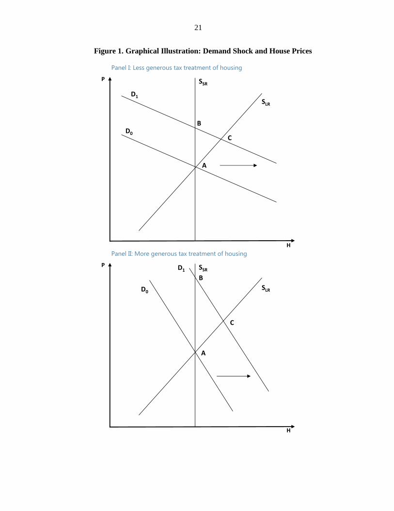
Figure 1 provides graphical illustration of how demand shock affects house prices in the

presence of different property tax systems. Panel I shows the results for less generous tax

treatment of housing (flatter demand curve), while Panel II depicts the case of a more

generous tax treatment (steeper demand curve). Given the inelastic short-term supply curve

(horizontal line SSR), the equilibrium initially moves from A to B. Over time, the supply

would expand (upward-slopping line SLR) and equilibrium would be set at C. Overall, prices

first go up and then come down, settling at a higher level than that prior to the shock. The

key implication is that the volatility of house prices (or overshooting) during this transition is

larger in the presence of a more generous tax treatment.

7

Assuming that the expected house price inflation is a linear function of the observed price

change in the previous period (E[dPt/dt]=a*[Pt-1-Pt-2], with a>0)6 and abstracting away from

capital gains taxes (c=0), equation (1) can be rewritten as:

𝑃𝑡 =𝑎

𝑟∙(1−𝜏𝑚)+𝜏𝑝+𝛿∙ (𝑃𝑡−1 − 𝑃𝑡−2) +

𝑅𝑡

𝑟∙(1−𝜏𝑚)+𝜏𝑝+𝛿 (3)

where r (1-m)+ p + > 0 and a>0.

Specification (3) indicates that after an initial demand shock to R, the accelerator mechanism

sets in assuming unchanged supply. This mechanism will be stronger for lower property tax

rates (smaller m). The equation will produce an oscillating development of the price level

and its rate of change, with the amplitude greater for higher values of the ratio a/[r (1-m)+

p + +].

In sum, this simple theoretical model suggests that lower property tax rates will lead to

higher volatility of house prices following an exogenous demand shock. In the long-run

(equilibrium), the property tax rate itself does not induce the price volatility, but can

exacerbate or dampen the impact of shocks. In the short-run, property tax rate changes can

contribute to house price volatility directly as prices adjust to the new equilibrium.

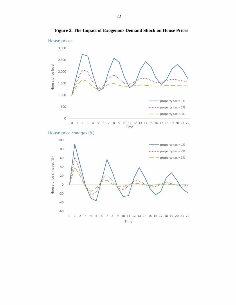
Figure 2 illustrates the dynamics of house prices in response to a permanent demand shock.

As expected, the volatility of house prices in response to a shock is higher for lower levels of

property taxes. We test the empirical validity of this theoretical prediction below.

III. DATA AND DESCRIPTIVE STATISTICS

A. Data

Our database covers the period 2005-2014. We employ separately data on 51 U.S. states and

77 MSAs in two sets of regressions. Table 1 lists variables and their sources.

House price data are taken from the Federal Housing Finance Agency. Annual house prices

are estimated as averages of four quarters within a year. Macroeconomic variables, including

nominal and real GDP, GDP deflator, per capita GDP, and population are taken from the

Bureau of Economic Analysis. Effective property tax rates are measured as the ratio of the

median annual property tax payment to the median property value for owner-occupied

housing units. Both series are taken from the American Community Survey maintained by

the Census. The advantage of this measure is that it accounts for differences in property tax

rates across counties within the state and property tax exemptions/adjustments.

Unfortunately, the survey data do not extend back beyond 2005, so the series are restricted to

the 2005-2014 period.

6 This assumption suggests that after a positive demand shock has produced first-round effect on house prices,

households may anticipate further price increases. It also implies that property taxes do not directly affect

expected house price changes.

(continued…)

8

The volatility of house prices is estimated using 5-year backward moving window. We use

the following alternative measures of real house prices for estimating volatility: (i) annual

growth rates, and (ii) percentage deviations from the HP-filtered value.7

B. Descriptive Statistics

Table 2 presents descriptive statistics of all variables used in the analysis. The panel is

balanced, with 510 state-year and 770 MSA-year observations. The average effective

property tax rate in the sample is 1 percent, with standard deviation of 0.5 percent. The

average volatility of house prices is 5-6 percent, depending on the measure.

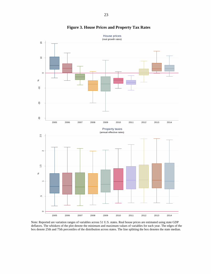
Figure 3 presents the dynamics of house price growth rates and property taxes across 51 U.S.

states over 1995-2014. Two observations are worth noting. First, the median house price

growth rate has switched from positive to negative during the crisis period (2007-11). For

each year, the real growth rates varied widely across states, with 25-75 interquartile range of

up to 8 percent depending on the year. The variation across states was largest at the height of

the crisis in 2009, when some states have experienced positive growth rates despite the

negative median. This suggests that some states managed to weather the demand shock better

than others and property tax rates could have played a role here. Second, the median effective

property tax rate has increased from 0.8 percent before the crisis to 1 percent now. This was

in part driven by the large deficits run by local governments requiring them to look for

alternative revenue sources to meet their balanced budget targets (Gracia et al., 2014).

Similar to house prices, effective property tax rates vary widely across states and this

variation did not change following the crisis. In some states, property tax rates are

approaching 2.5 percent level, with the 25-75 interquartile range reaching up to 1 percent

depending on the year.

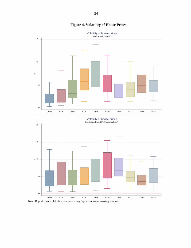
Figure 4 presents the dynamics of house price volatility using both definitions. Both

measures provide a qualitatively similar picture. The median state standard deviation has

increased from below 5 percent to above 5 percent during the crisis. There is wide variation

across states, exceeding 15 percent in some years. The standard deviation has declined back

to pre-crisis levels recently.

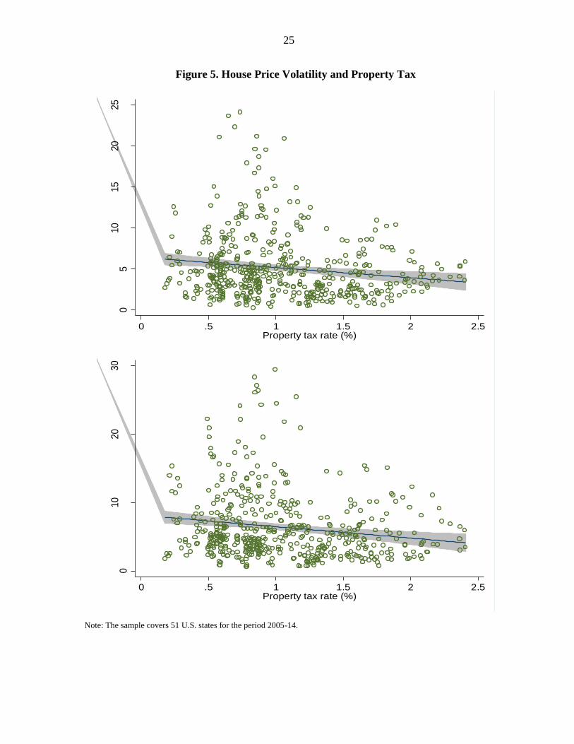
Figure 5 presents simple scatterplots of house price volatility and property tax rates. The

slopes are negative for both definitions of house price volatility, suggesting a lower volatility

in state-years characterized by high property tax rates. There is also some evidence of

heteroscedasticity, with distribution of house price volatility being larger in state-years with

low property tax rates. The latter suggests that robust standard errors should be used in the

regressions to improve inference.

7 Following the established practice for annual series, the smoothing parameter of the HP filter is set to 100.

9

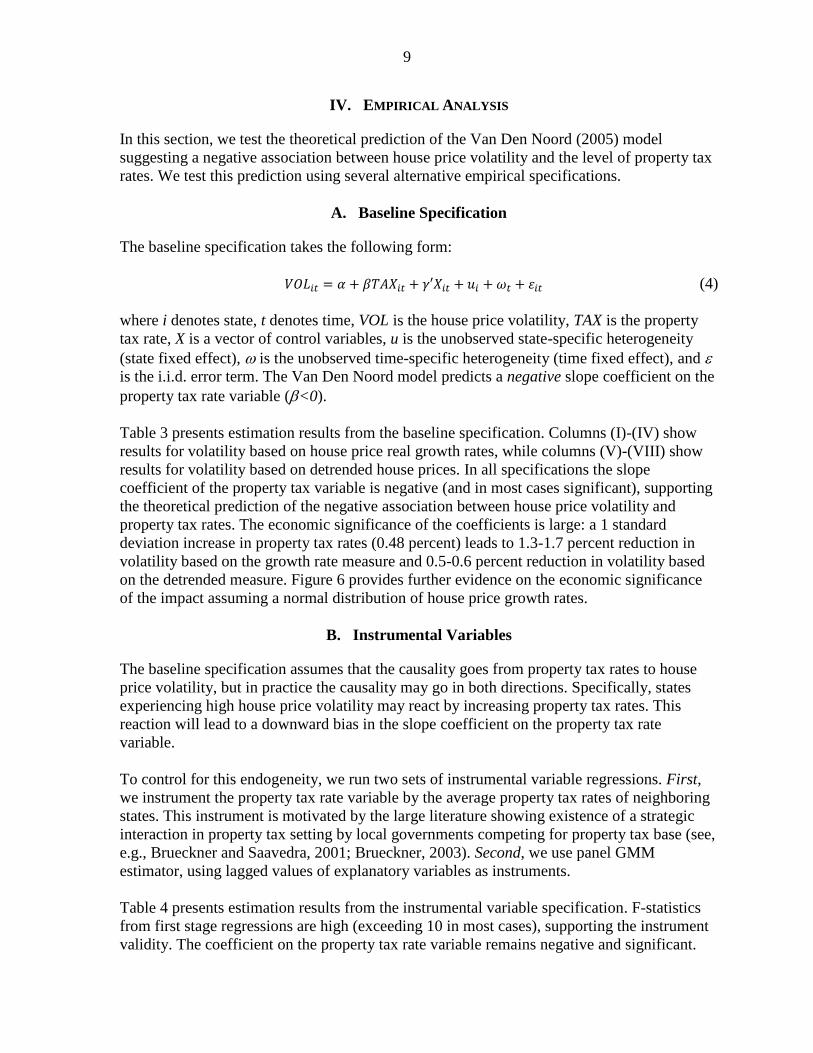
IV. EMPIRICAL ANALYSIS

In this section, we test the theoretical prediction of the Van Den Noord (2005) model

suggesting a negative association between house price volatility and the level of property tax

rates. We test this prediction using several alternative empirical specifications.

A. Baseline Specification

The baseline specification takes the following form:

𝑉𝑂𝐿𝑖𝑡 = 𝛼 + 𝛽𝑇𝐴𝑋𝑖𝑡 + 𝛾′𝑋𝑖𝑡 + 𝑢𝑖 + 𝜔𝑡 + 휀𝑖𝑡 (4)

where i denotes state, t denotes time, VOL is the house price volatility, TAX is the property

tax rate, X is a vector of control variables, u is the unobserved state-specific heterogeneity

(state fixed effect), is the unobserved time-specific heterogeneity (time fixed effect), and is the i.i.d. error term. The Van Den Noord model predicts a negative slope coefficient on the

property tax rate variable (<0).

Table 3 presents estimation results from the baseline specification. Columns (I)-(IV) show

results for volatility based on house price real growth rates, while columns (V)-(VIII) show

results for volatility based on detrended house prices. In all specifications the slope

coefficient of the property tax variable is negative (and in most cases significant), supporting

the theoretical prediction of the negative association between house price volatility and

property tax rates. The economic significance of the coefficients is large: a 1 standard

deviation increase in property tax rates (0.48 percent) leads to 1.3-1.7 percent reduction in

volatility based on the growth rate measure and 0.5-0.6 percent reduction in volatility based

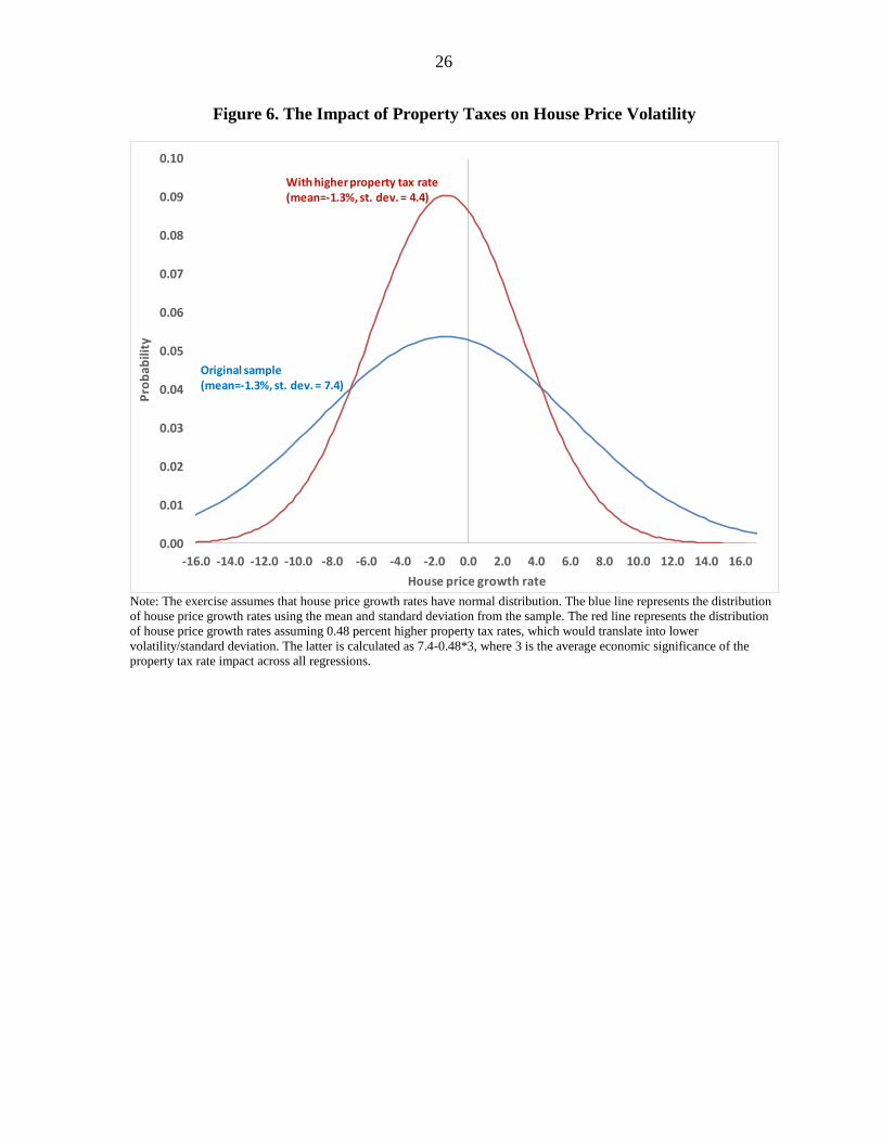
on the detrended measure. Figure 6 provides further evidence on the economic significance

of the impact assuming a normal distribution of house price growth rates.

B. Instrumental Variables

The baseline specification assumes that the causality goes from property tax rates to house

price volatility, but in practice the causality may go in both directions. Specifically, states

experiencing high house price volatility may react by increasing property tax rates. This

reaction will lead to a downward bias in the slope coefficient on the property tax rate

variable.

To control for this endogeneity, we run two sets of instrumental variable regressions. First,

we instrument the property tax rate variable by the average property tax rates of neighboring

states. This instrument is motivated by the large literature showing existence of a strategic

interaction in property tax setting by local governments competing for property tax base (see,

e.g., Brueckner and Saavedra, 2001; Brueckner, 2003). Second, we use panel GMM

estimator, using lagged values of explanatory variables as instruments.

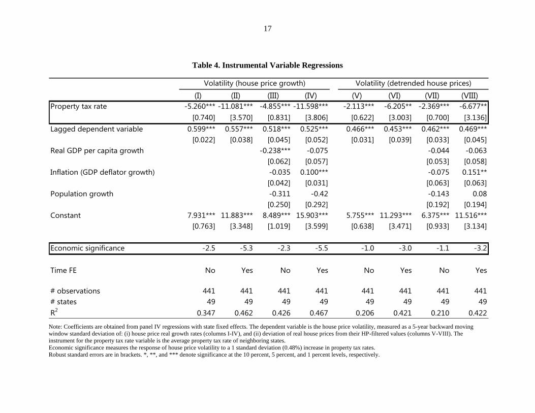
Table 4 presents estimation results from the instrumental variable specification. F-statistics

from first stage regressions are high (exceeding 10 in most cases), supporting the instrument

validity. The coefficient on the property tax rate variable remains negative and significant.

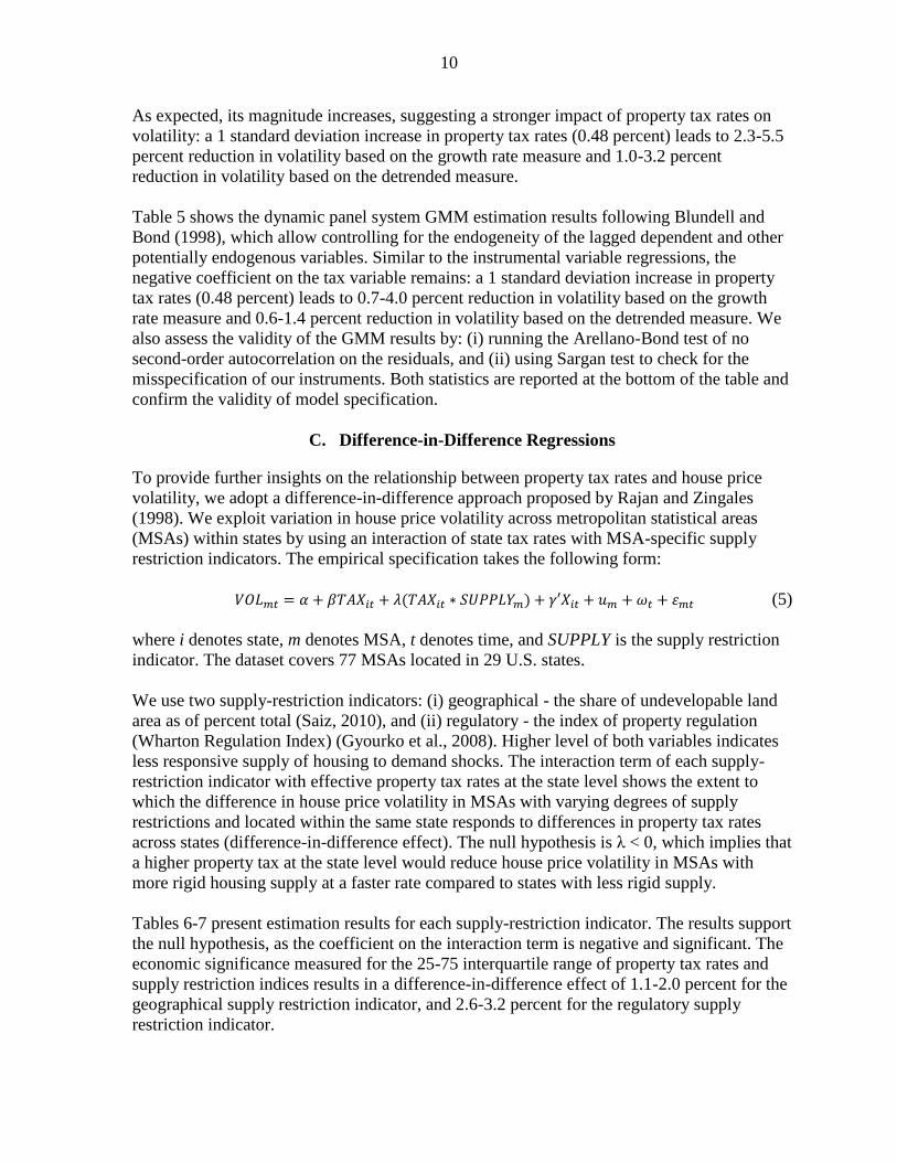
10

As expected, its magnitude increases, suggesting a stronger impact of property tax rates on

volatility: a 1 standard deviation increase in property tax rates (0.48 percent) leads to 2.3-5.5

percent reduction in volatility based on the growth rate measure and 1.0-3.2 percent

reduction in volatility based on the detrended measure.

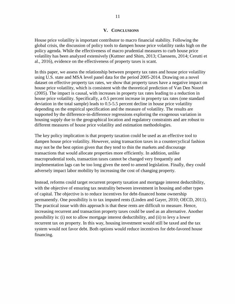
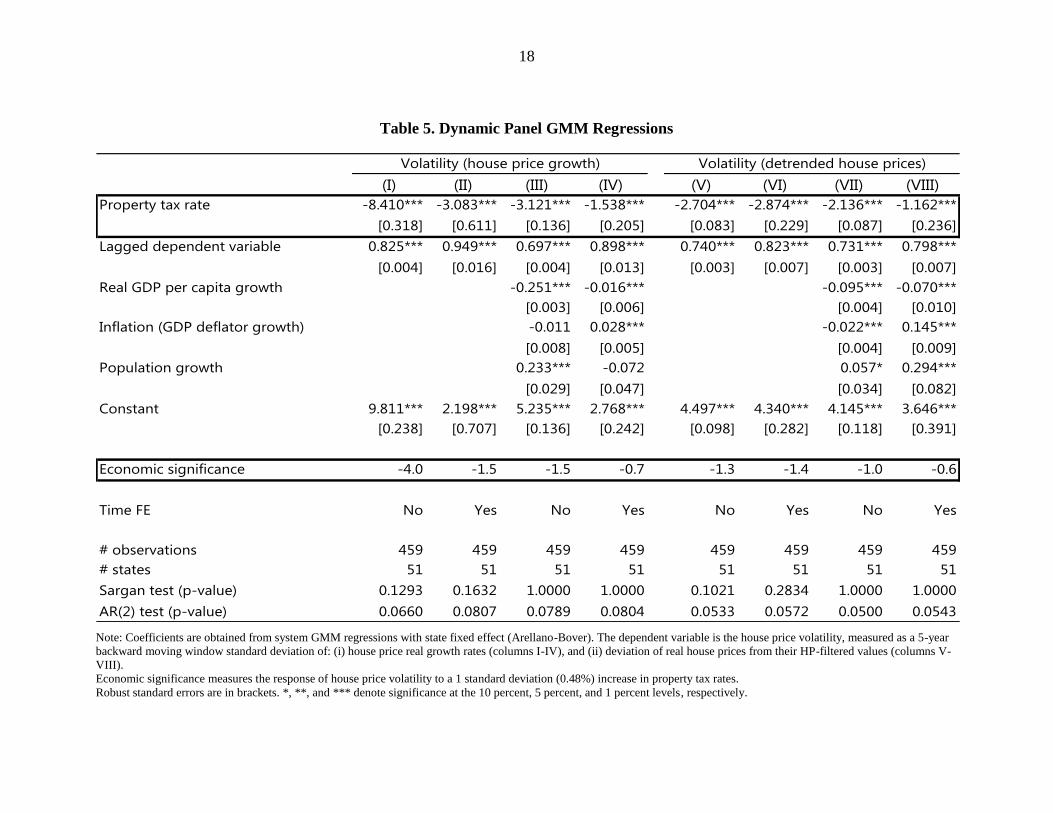
Table 5 shows the dynamic panel system GMM estimation results following Blundell and

Bond (1998), which allow controlling for the endogeneity of the lagged dependent and other

potentially endogenous variables. Similar to the instrumental variable regressions, the

negative coefficient on the tax variable remains: a 1 standard deviation increase in property

tax rates (0.48 percent) leads to 0.7-4.0 percent reduction in volatility based on the growth

rate measure and 0.6-1.4 percent reduction in volatility based on the detrended measure. We

also assess the validity of the GMM results by: (i) running the Arellano-Bond test of no

second-order autocorrelation on the residuals, and (ii) using Sargan test to check for the

misspecification of our instruments. Both statistics are reported at the bottom of the table and

confirm the validity of model specification.

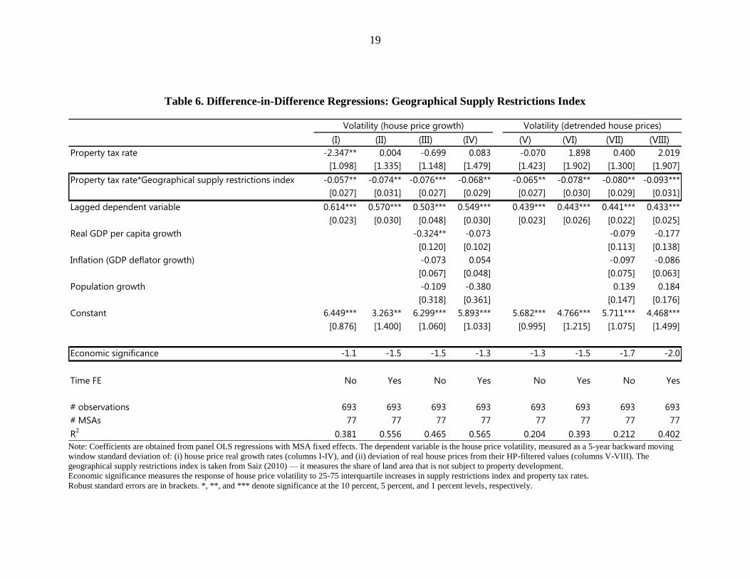
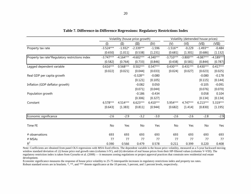
C. Difference-in-Difference Regressions

To provide further insights on the relationship between property tax rates and house price

volatility, we adopt a difference-in-difference approach proposed by Rajan and Zingales

(1998). We exploit variation in house price volatility across metropolitan statistical areas

(MSAs) within states by using an interaction of state tax rates with MSA-specific supply

restriction indicators. The empirical specification takes the following form:

𝑉𝑂𝐿𝑚𝑡 = 𝛼 + 𝛽𝑇𝐴𝑋𝑖𝑡 + 𝜆(𝑇𝐴𝑋𝑖𝑡 ∗ 𝑆𝑈𝑃𝑃𝐿𝑌𝑚) + 𝛾′𝑋𝑖𝑡 + 𝑢𝑚 + 𝜔𝑡 + 휀𝑚𝑡 (5)

where i denotes state, m denotes MSA, t denotes time, and SUPPLY is the supply restriction

indicator. The dataset covers 77 MSAs located in 29 U.S. states.

We use two supply-restriction indicators: (i) geographical - the share of undevelopable land

area as of percent total (Saiz, 2010), and (ii) regulatory - the index of property regulation

(Wharton Regulation Index) (Gyourko et al., 2008). Higher level of both variables indicates

less responsive supply of housing to demand shocks. The interaction term of each supply-

restriction indicator with effective property tax rates at the state level shows the extent to

which the difference in house price volatility in MSAs with varying degrees of supply

restrictions and located within the same state responds to differences in property tax rates

across states (difference-in-difference effect). The null hypothesis is λ < 0, which implies that

a higher property tax at the state level would reduce house price volatility in MSAs with

more rigid housing supply at a faster rate compared to states with less rigid supply.

Tables 6-7 present estimation results for each supply-restriction indicator. The results support

the null hypothesis, as the coefficient on the interaction term is negative and significant. The

economic significance measured for the 25-75 interquartile range of property tax rates and

supply restriction indices results in a difference-in-difference effect of 1.1-2.0 percent for the

geographical supply restriction indicator, and 2.6-3.2 percent for the regulatory supply

restriction indicator.

11

V. CONCLUSIONS

House price volatility is important contributor to macro financial stability. Following the

global crisis, the discussion of policy tools to dampen house price volatility ranks high on the

policy agenda. While the effectiveness of macro prudential measures to curb house price

volatility has been analyzed extensively (Kuttner and Shim, 2013; Claessens, 2014; Cerutti et

al., 2016), evidence on the effectiveness of property taxes is scant.

In this paper, we assess the relationship between property tax rates and house price volatility

using U.S. state and MSA level panel data for the period 2005-2014. Drawing on a novel

dataset on effective property tax rates, we show that property taxes have a negative impact on

house price volatility, which is consistent with the theoretical prediction of Van Den Noord

(2005). The impact is causal, with increases in property tax rates leading to a reduction in

house price volatility. Specifically, a 0.5 percent increase in property tax rates (one standard

deviation in the total sample) leads to 0.5-5.5 percent decline in house price volatility

depending on the empirical specification and the measure of volatility. The results are

supported by the difference-in-difference regressions exploring the exogenous variation in

housing supply due to the geographical location and regulatory constraints and are robust to

different measures of house price volatility and estimation methodologies.

The key policy implication is that property taxation could be used as an effective tool to

dampen house price volatility. However, using transaction taxes in a countercyclical fashion

may not be the best option given that they tend to thin the markets and discourage

transactions that would allocate properties more efficiently. In addition, unlike

macroprudential tools, transaction taxes cannot be changed very frequently and

implementation lags can be too long given the need to amend legislation. Finally, they could

adversely impact labor mobility by increasing the cost of changing property.

Instead, reforms could target recurrent property taxation and mortgage interest deductibility,

with the objective of ensuring tax neutrality between investment in housing and other types

of capital. The objective is to reduce incentives for debt-financed home ownership

permanently. One possibility is to tax imputed rents (Linden and Gayer, 2010; OECD, 2011).

The practical issue with this approach is that these rents are difficult to measure. Hence,

increasing recurrent and transaction property taxes could be used as an alternative. Another

possibility is: (i) not to allow mortgage interest deductibility, and (ii) to levy a lower

recurrent tax on property. In this way, housing investment would still be taxed and the tax

system would not favor debt. Both options would reduce incentives for debt-favored house

financing.

12

REFERENCES

Andrews, D., 2010, “Real House Prices in OECD Countries: The Role of Demand Shocks

and Structural and Policy Factors,” OECD Economics Department Working Papers,

No. 831 (Paris: OECD).

Andrews, D., A. Caldera Sanchez, and A. Johansson, 2011, "Housing markets and structural

policies in OECD countries", OECD Economics Department Working papers, No.

836 (Paris: OECD).

Aregger, N., M. Brown and E. Ross, 2013, “Transaction Taxes, Capital Gains Taxes, and

House Prices,” Swiss National Bank Working Paper No. 2 (Zurich: Swiss National

Bank).

Brueckner, J., 2003, “Strategic Interaction among Governments: An Overview of Empirical

Studies,” International Regional Science Review, 26: pp. 175-188.

Brueckner, J. and L. Saavedra, 2001, “Do Local Governments Engage in Strategic Property-

Tax Competition,” National Tax Journal, 54 (2): pp. 203-30.

Cerutti, E., S. Claessens, and L. Laeven, 2016, “The Use and Effectiveness of

Macroprudential Policies: New Evidence,” Journal of Financial Stability

(forthcoming, also IMF WP 15/61).

Claessens, S., 2015, “An Overview of Macroprudential Policy Tools,” IMF Working Paper

WP/14/214 (Washington, D.C.: International Monetary Fund).

Crowe, C., G. Dell’Ariccia, D. Igan, and P. Rabanal, 2013, “How to Deal with Real Estate

Booms: Lessons from Country Experiences,” Journal of Financial Stability, 9: pp.

300-319.

Darbar, S., and X. Wu, 2015, “Experiences with Macroeconomic Policy – Five Case

Studies,” IMF Working Paper WP/15/123 (Washington, D.C.: International Monetary

Fund).

Gattini, L., and I. Ganoulis, 2012, “House Price Responsiveness of Housing Investments

Across Major European Economies,” ECB Working Paper No. 1461 (Frankfurt:

European Central Bank).

Gracia, B., J. McHugh, and T. Poghosyan, 2014, “Impact of the Crisis and Policy Response

at the Sub-National Level,” in: Cottarelli, C., P. Gerson, and A. Senhadji (eds.), Post-

Crisis Fiscal Policy, (Cambridge: MIT Press).

Gyourko, J., A. Saiz, and A. Summers, 2008, “A New Measure of the Local Regulatory

Environment for Housing Markets: The Wharton Residential Land Use Regulatory

Index,” Urban Studies, 45: pp. 693–729.

13

He, D. 2014. “The Effects of Macroprudential Policies on Housing Market Risks: Evidence

from Hong Kong.” Banque de France, Financial Stability Review No. 18 (April).

Hilber, C. and W. Vermeulen, 2016, “The Impact of Supply Constraints on House Prices in

England,” The Economic Journal (forthcoming).

IMF. 2013. “Fiscal Monitor: Taxing Times”, October.

Lim, C., F. Columba, A. Costa, P. Kongsamut, A. Otani, M. Saiyid, T. Wezel, and X. Wu.

2011. “Macroprudential Policy: What Instruments and How to Use Them?” IMF

Working Paper WP/11/238 (Washington, D.C.: International Monetary Fund).

Linden, A. J. and C. Gayer. 2012. “Possible Reforms of Real Estate Taxation: Criteria for

Successful Policies.” European Economy, Occasional Paper No 119.

Norregaard, J., 2015, “Taxing Immovable Property: Revenue Potential and Implementation

Challenges,” IMF Working Paper WP/13/129 (Washington, D.C.: International

Monetary Fund).

OECD, 2011, “Housing and the Economy: Policies for Renovation,” Chapter 4 in Economic

Policy Reforms 2011: Going for Growth (Paris: OECD).

Poterba, J., 1992, “Taxation and Housing: Old Questions, New Answers,” American

Economic Review, 82 (2): 237-242.

Poterba, J. and T. Sinai, 2008, “Tax Expenditures for Owner Occupied Housing: Deduction

for Property Taxes and Mortgage Interest and the Exclusion of Imputed Rental

Income,” American Economic Review P&P, 98 (2): 84-89.

Keen, M., A. Klemm, and V. Perry. 2010. “Tax and the Crisis.” Fiscal Studies, 31 (1), pp.

43-79.

Kuttner, K. and I. Shim, 2013, “Can Non-Interest Rate Policies Stabilize Housing Markets?

Evidence from a Panel of 57 Economies,” BIS Working Papers No. 433 (Basel: BIS).

Rajan, R., and L. Zingales, 1998, “Financial Dependence and Growth,” American Economic

Review, 88 (3): pp. 559-586.

Saiz, A., 2010, “The Geographic Determinants of Housing Supply,” The Quarterly Journal

of Economics, 125 (3): pp. 1253-96.

Van Den Noord, P., 2005, “Tax Incentives and House Price Volatility in the Euro Area:

Theory and Evidence,” Economie Internationale, 101: pp. 29-45.

14

Table 1. Variables and Data Sources

Variable Definition Frequency Geography Source

House prices Weighted repeated-sales indices of single family house

prices (seasonally adjusted and non-adjusted)

Quarterly State, MSA Federal Housing

Finance Agency

Property tax rate Effective rate = 100*Property taxes paid/Assessed value

of the house (state median)

Annual State, MSA Census bureau

Nominal GDP Value added of all industries (current prices) Annual State Bureau of Economic

Analysis

Real GDP Value added of all industries (constant prices) Annual State Bureau of Economic

Analysis

GDP deflator Ratio of nominal and real GDP Annual State Bureau of Economic

Analysis

Real per capita GDP Value added of all industries (constant prices)/Population Annual State Bureau of Economic

Analysis

Population Number of state residents Annual State Bureau of Economic

Analysis

Geographical restrictions index Share of undevelopable geographical area Annual MSA Saiz (2010)

Regulatory restrictions index Index measuring zoning regulations or project

approval practices that constrain new residential real

estate development

Annual MSA Gyorko et al. (2008)

House prices

Property tax rates

Macro variables

Housing Supply Restrictions

15

Table 2. Descriptive Statistics

Obs. Mean Median St. Dev. 10th percentile 90th percentile 25th percentile 75th percentile

Hose price growth rate (%) 510 -1.30 -0.95 7.42 -9.67 6.94 -5.57 2.98

Effective property tax rate (%) 510 1.04 0.91 0.48 0.52 1.75 0.65 1.35

House price volatility (%, growth-based) 510 5.13 4.18 3.90 1.55 10.28 2.47 6.28

House price volatility (%, HP-based) 510 6.39 4.92 4.93 1.96 12.85 3.16 8.15

Real GDP per capita growth (%) 510 1.27 1.40 2.66 -1.69 4.16 0.16 2.54

GDP deflator growth (%) 510 2.23 2.10 1.88 1.09 3.50 1.67 2.84

Population growth (%) 510 0.84 0.75 0.75 0.11 1.73 0.35 1.24

Supply restrictions index (Saiz, 2010) 770 27.94 23.29 22.32 3.12 64.01 9.28 40.50

Regulatory restrictions index (Wharton) 770 0.10 0.03 0.69 -0.81 0.94 -0.38 0.61

16

Table 3. Baseline Regressions

(I) (II) (III) (IV) (V) (VI) (VII) (VIII)

Property tax rate -3.542*** -2.784*** -3.210*** -2.802*** -1.283** -1.111 -1.347** -1.177

[0.674] [0.884] [0.789] [0.893] [0.610] [0.750] [0.626] [0.746]

Lagged dependent variable 0.579*** 0.551*** 0.497*** 0.526*** 0.466*** 0.462*** 0.465*** 0.474***

[0.022] [0.033] [0.042] [0.046] [0.033] [0.041] [0.035] [0.047]

Real GDP per capita growth -0.239*** -0.048 -0.052 -0.038

[0.064] [0.052] [0.053] [0.057]

Inflation (GDP deflator growth) -0.067 0.023 -0.048 0.091*

[0.050] [0.041] [0.039] [0.049]

Population growth -0.165 -0.363* -0.026 0.069

[0.209] [0.208] [0.160] [0.120]

Constant 6.186*** 4.122*** 6.792*** 6.952*** 4.861*** 5.734*** 5.113*** 5.971***

[0.699] [0.880] [0.976] [1.002] [0.602] [0.895] [0.721] [0.800]

Economic significance -1.7 -1.3 -1.5 -1.3 -0.6 -0.5 -0.6 -0.6

Time FE No Yes No Yes No Yes No Yes

# observations 459 459 459 459 459 459 459 459

# states 51 51 51 51 51 51 51 51

R2

0.365 0.588 0.434 0.598 0.215 0.460 0.219 0.465

Volatility (house price growth) Volatility (detrended house prices)

17

Table 4. Instrumental Variable Regressions

Note: Coefficients are obtained from panel IV regressions with state fixed effects. The dependent variable is the house price volatility, measured as a 5-year backward moving

window standard deviation of: (i) house price real growth rates (columns I-IV), and (ii) deviation of real house prices from their HP-filtered values (columns V-VIII). The

instrument for the property tax rate variable is the average property tax rate of neighboring states.

Economic significance measures the response of house price volatility to a 1 standard deviation (0.48%) increase in property tax rates.

Robust standard errors are in brackets. *, **, and *** denote significance at the 10 percent, 5 percent, and 1 percent levels, respectively.


Property tax rate -5.260*** -11.081*** -4.855*** -11.598*** -2.113*** -6.205** -2.369*** -6.677**

[0.740] [3.570] [0.831] [3.806] [0.622] [3.003] [0.700] [3.136]


[0.022] [0.038] [0.045] [0.052] [0.031] [0.039] [0.033] [0.045]

Real GDP per capita growth -0.238*** -0.075 -0.044 -0.063

[0.062] [0.057] [0.053] [0.058]

Inflation (GDP deflator growth) -0.035 0.100*** -0.075 0.151**

[0.042] [0.031] [0.063] [0.063]

Population growth -0.311 -0.42 -0.143 0.08

[0.250] [0.292] [0.192] [0.194]

Constant 7.931*** 11.883*** 8.489*** 15.903*** 5.755*** 11.293*** 6.375*** 11.516***

[0.763] [3.348] [1.019] [3.599] [0.638] [3.471] [0.933] [3.134]



# observations 441 441 441 441 441 441 441 441

# states 49 49 49 49 49 49 49 49

R2

0.347 0.462 0.426 0.467 0.206 0.421 0.210 0.422


18

Table 5. Dynamic Panel GMM Regressions

Note: Coefficients are obtained from system GMM regressions with state fixed effect (Arellano-Bover). The dependent variable is the house price volatility, measured as a 5-year

backward moving window standard deviation of: (i) house price real growth rates (columns I-IV), and (ii) deviation of real house prices from their HP-filtered values (columns V-

VIII).

Economic significance measures the response of house price volatility to a 1 standard deviation (0.48%) increase in property tax rates.



Property tax rate -8.410*** -3.083*** -3.121*** -1.538*** -2.704*** -2.874*** -2.136*** -1.162***

[0.318] [0.611] [0.136] [0.205] [0.083] [0.229] [0.087] [0.236]


[0.004] [0.016] [0.004] [0.013] [0.003] [0.007] [0.003] [0.007]

Real GDP per capita growth -0.251*** -0.016*** -0.095*** -0.070***

[0.003] [0.006] [0.004] [0.010]

Inflation (GDP deflator growth) -0.011 0.028*** -0.022*** 0.145***

[0.008] [0.005] [0.004] [0.009]

Population growth 0.233*** -0.072 0.057* 0.294***

[0.029] [0.047] [0.034] [0.082]

Constant 9.811*** 2.198*** 5.235*** 2.768*** 4.497*** 4.340*** 4.145*** 3.646***

[0.238] [0.707] [0.136] [0.242] [0.098] [0.282] [0.118] [0.391]



# observations 459 459 459 459 459 459 459 459

# states 51 51 51 51 51 51 51 51

Sargan test (p-value) 0.1293 0.1632 1.0000 1.0000 0.1021 0.2834 1.0000 1.0000

AR(2) test (p-value) 0.0660 0.0807 0.0789 0.0804 0.0533 0.0572 0.0500 0.0543

Volatility (detrended house prices)Volatility (house price growth)

19

Table 6. Difference-in-Difference Regressions: Geographical Supply Restrictions Index

Note: Coefficients are obtained from panel OLS regressions with MSA fixed effects. The dependent variable is the house price volatility, measured as a 5-year backward moving


geographical supply restrictions index is taken from Saiz (2010) — it measures the share of land area that is not subject to property development.

Economic significance measures the response of house price volatility to 25-75 interquartile increases in supply restrictions index and property tax rates.



Property tax rate -2.347** 0.004 -0.699 0.083 -0.070 1.898 0.400 2.019

[1.098] [1.335] [1.148] [1.479] [1.423] [1.902] [1.300] [1.907]

Property tax rate*Geographical supply restrictions index -0.057** -0.074** -0.076*** -0.068** -0.065** -0.078** -0.080** -0.093***

[0.027] [0.031] [0.027] [0.029] [0.027] [0.030] [0.029] [0.031]


[0.023] [0.030] [0.048] [0.030] [0.023] [0.026] [0.022] [0.025]

Real GDP per capita growth -0.324** -0.073 -0.079 -0.177

[0.120] [0.102] [0.113] [0.138]

Inflation (GDP deflator growth) -0.073 0.054 -0.097 -0.086

[0.067] [0.048] [0.075] [0.063]

Population growth -0.109 -0.380 0.139 0.184

[0.318] [0.361] [0.147] [0.176]

Constant 6.449*** 3.263** 6.299*** 5.893*** 5.682*** 4.766*** 5.711*** 4.468***

[0.876] [1.400] [1.060] [1.033] [0.995] [1.215] [1.075] [1.499]



# observations 693 693 693 693 693 693 693 693

# MSAs 77 77 77 77 77 77 77 77

R2

0.381 0.556 0.465 0.565 0.204 0.393 0.212 0.402


20

Table 7. Difference-in-Difference Regressions: Regulatory Restrictions Index

Note: Coefficients are obtained from panel OLS regressions with MSA fixed effects. The dependent variable is the house price volatility, measured as a 5-year backward moving


regulatory restriction index is taken from Gyourko et al. (2008) — it measures zoning regulations or project approval practices that constrain new residential real estate

development.

Economic significance measures the response of house price volatility to 25-75 interquartile increases in regulatory restrictions index and property tax rates.



Property tax rate -3.524*** -1.932* -2.339*** -1.596 -1.516** -0.229 -1.493** -0.484

[0.650] [1.011] [0.538] [1.231] [0.681] [1.301] [0.686] [1.132]

Property tax rate*Regulatory restrictions index -3.747*** -4.164*** -4.602*** -4.340*** -3.710*** -3.800*** -4.087*** -4.189***

[0.582] [0.764] [0.733] [0.846] [0.438] [0.581] [0.844] [0.787]


[0.022] [0.021] [0.044] [0.033] [0.024] [0.027] [0.023] [0.025]

Real GDP per capita growth -0.328** -0.080 -0.080 -0.178

[0.121] [0.105] [0.115] [0.144]

Inflation (GDP deflator growth) -0.082 0.050 -0.105 -0.091

[0.071] [0.044] [0.076] [0.070]

Population growth -0.186 -0.434 0.058 0.104

[0.306] [0.327] [0.134] [0.134]

Constant 6.578*** 4.514*** 6.623*** 6.410*** 5.954*** 4.747*** 6.213*** 5.319***

[0.643] [1.383] [0.811] [0.944] [0.682] [1.414] [0.830] [1.195]



# observations 693 693 693 693 693 693 693 693

# MSAs 77 77 77 77 77 77 77 77

R2

0.390 0.566 0.479 0.578 0.211 0.399 0.220 0.408


21

Figure 1. Graphical Illustration: Demand Shock and House Prices

Panel I: Less generous tax treatment of housing

P

H

Panel II: More generous tax treatment of housing

P

H

A

B

CD0

D1

SSR

SLR

A

B

C

D0

D1 SSR

SLR

22

Figure 2. The Impact of Exogenous Demand Shock on House Prices

House prices

House price changes (%)

0

500

1,000

1,500

2,000

2,500

3,000

0 1 2 3 4 5 6 7 8 9 10 11 12 13 14 15 16 17 18 19 20 21 22

Ho

use

pri

ce le

vel

Time

property tax = 1%

property tax = 2%

property tax = 3%

-60

-40

-20

0

20

40

60

80

100

0 1 2 3 4 5 6 7 8 9 10 11 12 13 14 15 16 17 18 19 20 21 22

Ho

use

pri

ce c

hn

ages

(%

)

Time

property tax = 1%

property tax = 2%

property tax = 3%

23

Figure 3. House Prices and Property Tax Rates

Note: Reported are variation ranges of variables across 51 U.S. states. Real house prices are estimated using state GDP

deflators. The whiskers of the plot denote the minimum and maximum values of variables for each year. The edges of the

box denote 25th and 75th percentiles of the distribution across states. The line splitting the box denotes the state median.

0.5

11

.52

2.5

%

2005 2006 2007 2008 2009 2010 2011 2012 2013 2014

(annual effective rates)

Property taxes

-30

-20

-10

01

02

0

%

2005 2006 2007 2008 2009 2010 2011 2012 2013 2014

(real growth rates)

House prices

24

Figure 4. Volatility of House Prices

Note: Reported are volatilities measures using 5-year backward moving window.

05

10

15

%

2005 2006 2007 2008 2009 2010 2011 2012 2013 2014

(real growth rates)

Volatility of house prices

05

10

15

20

%

2005 2006 2007 2008 2009 2010 2011 2012 2013 2014

(deviation from HP-filtered values)

Volatility of house prices

25

Figure 5. House Price Volatility and Property Tax

Note: The sample covers 51 U.S. states for the period 2005-14.

010

20

30

Ho

use

price

vo

latil

ity (

detr

en

de

d)

0 .5 1 1.5 2 2.5Property tax rate (%)

05

10

15

20

25

Ho

use

price

vo

latil

ity (

gro

wth

ra

te)

0 .5 1 1.5 2 2.5Property tax rate (%)

26

Figure 6. The Impact of Property Taxes on House Price Volatility

Note: The exercise assumes that house price growth rates have normal distribution. The blue line represents the distribution

of house price growth rates using the mean and standard deviation from the sample. The red line represents the distribution

of house price growth rates assuming 0.48 percent higher property tax rates, which would translate into lower

volatility/standard deviation. The latter is calculated as 7.4-0.48*3, where 3 is the average economic significance of the

property tax rate impact across all regressions.

0.00

0.01

0.02

0.03

0.04

0.05

0.06

0.07

0.08

0.09

0.10

-16.0 -14.0 -12.0 -10.0 -8.0 -6.0 -4.0 -2.0 0.0 2.0 4.0 6.0 8.0 10.0 12.0 14.0 16.0

Pro

bab

ility

House price growth rate

Original sample (mean=-1.3%, st. dev. = 7.4)

With higher property tax rate (mean=-1.3%, st. dev. = 4.4)

can property taxes reduce house price volatility? evidence from

Documents