can falling supply explain the rising return to college ... · can falling supply explain the...

Can Falling Supply Explain the Rising Return to College for Younger Men? A Cohort-BasedAnalysisAuthor(s): David Card and Thomas LemieuxSource: The Quarterly Journal of Economics, Vol. 116, No. 2 (May, 2001), pp. 705-746Published by: The MIT PressStable URL: http://www.jstor.org/stable/2696477Accessed: 06/10/2010 11:51

Your use of the JSTOR archive indicates your acceptance of JSTOR's Terms and Conditions of Use, available athttp://www.jstor.org/page/info/about/policies/terms.jsp. JSTOR's Terms and Conditions of Use provides, in part, that unlessyou have obtained prior permission, you may not download an entire issue of a journal or multiple copies of articles, and youmay use content in the JSTOR archive only for your personal, non-commercial use.

Please contact the publisher regarding any further use of this work. Publisher contact information may be obtained athttp://www.jstor.org/action/showPublisher?publisherCode=mitpress.

Each copy of any part of a JSTOR transmission must contain the same copyright notice that appears on the screen or printedpage of such transmission.

JSTOR is a not-for-profit service that helps scholars, researchers, and students discover, use, and build upon a wide range ofcontent in a trusted digital archive. We use information technology and tools to increase productivity and facilitate new formsof scholarship. For more information about JSTOR, please contact [email protected].

The MIT Press is collaborating with JSTOR to digitize, preserve and extend access to The Quarterly Journal ofEconomics.

http://www.jstor.org

http://www.jstor.org/action/showPublisher?publisherCode=mitpress

http://www.jstor.org/stable/2696477?origin=JSTOR-pdf

http://www.jstor.org/page/info/about/policies/terms.jsp

http://www.jstor.org/action/showPublisher?publisherCode=mitpress

CAN FALLING SUPPLY EXPLAIN THE RISING RETURN TO COLLEGE FOR YOUNGER MEN?

A COHORT-BASED ANALYSIS*

DAVID CARD AND THOMAS LEMIEUX

Although the college-high school wage gap for younger U. S. men has doubled over the past 30 years, the gap for older men has remained nearly constant. In the United Kingdom and Canada the college-high school wage gap also increased for younger relative to older men. Using a model with imperfect substitution between similarly educated workers in different age groups, we argue that these shifts reflect changes in the relative supply of highly educated workers across age groups. The driving force behind these changes is the slowdown in the rate of growth of educational attainment that began with cohorts born in the early 1950s in all three countries.

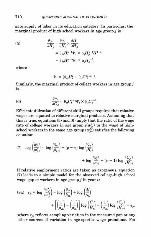
One of the most remarkable trends in the U. S. labor market is the rise in education-related wage differentials [Katz and Autor 1999]. Among men, for example, the gap in average earnings between workers with a college degree and those with only a high school diploma rose from about 25 percent in the mid-1970s to 40 percent in 1998. A less-known fact is that virtually the entire rise is attributable to changes in the relative earnings of younger college-educated workers. The top panel of Figure I, for example, plots the college-high school wage gap for younger (ages 26-35) and older (ages 46-60) men over the period from 1959 to 1996.1 While the earnings gap for young men has roughly doubled since 1975, the gap for older men is only slightly higher today than in the 1960s or 1970s. As a consequence of these divergent trends, the age structure of the college wage premium has shifted. In earlier years the gap between college and high-school educated workers increased steadily with age-as predicted by Mincer's [1974] human

* We are grateful to Alexandre Debs, David Lee, and Gena Estes for out- standing research assistance, and to David Green, Lawrence Katz, and two referees for helpful comments. Special thanks to Paul Beaudry for many helpful discussions. This research was supported by CIRANO, the Center for Labor Economics at the University of California at Berkeley, by SSHRC (Canada), and FCAR (Quebec) grants to Lemieux, and by an NICHD grant to Card through the National Bureau of Economic Research.

1. The data underlying this figure are based on average weekly earnings of full-time workers in the 1960 Census, and in March Current Population Surveys for 1970-1997.

? 2001 by the President and Fellows of Harvard College and the Massachusetts Institute of Technology. The Quarterly Journal of Economics, May 2001

705

706 QUARTERLY JOURNAL OF ECONOMICS

A. United States

0.5 -

0.4 Age 46-60 +- ---- O .4

- -- --- - -- --- --- ---- -- --- --- --

0.3

0.2 _

Age 26-30

0.1 -

0.0

1959 1970 1975 1980 1985 1990 1995

B. United Kingdom

0.5 i

04 - Age46-60

0.3 -

Age 26-30

0.2

0.1

0.0. 1959 1970 1975 1980 1985 1990 1995

C. Canada

0.5

0.4

Age 46-60 +- -. .

0.3

0.2

Age 26-30

0.1

0.0 1959 1970 1975 1980 1985 1990 1995

FIGURE I Estimated College-High School Wage Differentials for Younger and Older Men

CAN FALLING SUPPLY EXPLAIN THE RISING RETURN? 707

capital earnings function.2 Currently, however, the college premium is highest for men in their early thirties. As shown in the other panels of Figure I, a similar phenomenon has also occurred in the United Kingdom and Canada. In both countries the college-high school wage gap for younger men has risen, while the gap for older men has been stable or declining.

In this paper we explore a simple explanation for the trends in Figure I. We argue that the shifting structure of the returns to college in the United States, the United Kingdom, and Canada is a reflection of intercohort shifts in the relative supply of highly educated workers. The driving force behind these shifts is the slowdown in the rate of growth of educational attainment that began with cohorts born in the early 1950s. While conventional models of education-related wage differentials ignore differences in the age distribution of educational attainment, a simple exten- sion that incorporates imperfect substitutability between younger and older workers yields the prediction that a slowdown in the intercohort trend in educational attainment will lead to a relative rise in the college wage premium for younger workers that will slowly work its way through the age distribution as the cohort ages.

We evaluate this hypothesis using U. S. data on the college- high school wage gap for five year birth cohorts over the period from 1959 to 1996. As a check on our findings we also consider similar data from the United Kingdom over the period 1974- 1996, and from Canada over the period from 1980 to 1995. Al- though the three countries have very different levels of average educational attainment, all three show similar intercohort trends, with steadily rising educational attainments for cohorts born up to 1950, and relative stagnation for the baby-boom cohorts. Moreover, as suggested by the patterns in Figure I, the age structure of the college wage premium shows similar "twisting" in the three countries. Thus, there is prima facie evidence that the age structure of the college wage gap is related to the changing relative supply of more highly educated workers in different age

2. Mincer [19741 posited that the log of earnings depends on years of education and a quadratic function of labor market experience (age minus education minus five). This formulation implies that the difference in log wages between college and high school workers of the same age rises linearly with age. Recent research (e.g., Murphy and Welch [1990]) has allowed more flexible functions of experience, for example, log w = 3S + g(A - S - 5), where S = education and A = age. As long as g is concave and increasing, the implied college-high school wage gap is increasing with age.


groups. Indeed, our estimates of the elasticity of substitution between workers with the same education in different age groups are very similar for the three countries. Our findings suggest that shifts in cohort-specific supplies of highly educated workers, coupled with steadily increasing relative demand for educated workers, provide a unifying explanation for the observed changes in education-related wage differentials in all three countries.

I. THEORETICAL FRAMEWORK

A. A Model of Aggregate Production with Age-Group Specific Supplies

Although existing research on the rising return to higher education has emphasized the role of supply variation, most previous studies have focused on the average return to schooling, rather than differences by age or cohort (e.g., Freeman [1976], Freeman and Needels [1993], and Katz and Murphy [1992]).3 These studies analyze the evolution of the return to schooling under the assumption that different age groups with the same level of education are perfect substitutes in production. This assumption means that the aggregate supply of each "type" of education can be obtained by simply summing the total numbers of workers in each education category.4 A further simplification- which we will also invoke-is that there are only two education groups: "college equivalent" workers, and "high school equivalent" workers.5 Under these assumptions, all education-related wage differentials in the labor market in any given year are proportional to the average college-high school wage gap in that

3. One important exception is Murphy and Welch [1992] who develop and implement an alternative framework to analyze wage structure change allowing for factor supplies by experience and education group. They show that factor supply changes (by experience-education group) and demand changes (trend, unemployment, trade deficit) can explain the different evolution of wages in the United States by experience and education group for males from the early 1960s to late 1980s.

4. In practice, different age groups may be allowed to supply different efficiency units of labor, in which case a weighted average of the supply of workers in each age group is appropriate, with a weight equal to the relative wage of the group [Katz and Murphy 19921.

5. Following the literature (e.g., Johnson [1997]), we assume that workers with exactly a high school degree supply 1 high school equivalent; workers with exactly a college degree supply 1 college equivalent; workers with less than high school education supply some fraction of a high school equivalent; workers with an advanced degree supply more than 1 college equivalent; and workers with education qualifications between a high school and college degree supply oL high school equivalents and (1 - ot) college equivalents. See Section II for more details.


year. Moreover, the college wage gaps for different age groups will expand or contract proportionally over time, a prediction that is clearly inconsistent with recent movements in the United States, the United Kingdom, and Canada (see Figure I).

A natural way of relaxing the hypothesis of perfect substitution across age groups is to assume that aggregate output depends on two CES subaggregates of high-school and college labor:

vn

(1) [z=E (HaH ]t)j

and

(2) Ct=E(1jcit)

where -oo < q c 1 is a function of the partial elasticity of substitution UA between different age groups j with the same level of education (-q = 1 - 1/CA), and oj and 13j are relative efficiency parameters (assumed to be fixed over time). In principle, -r could be different for the two education groups, although we ignore this possibility for now to simplify our presentation of the model.6 We will relax this assumption in subsection III.C. In the limiting case of perfect substitutability across age groups, 'q is equal to 1 and total high-school (or college) labor input is just a weighted sum of the quantity of labor supplied by each age group.

Aggregate output in period t, Y, is a function of high school labor, college labor, and the technological efficiency parameters Oht and Oct:

(3) Yt = f(H,Ct;OhtAt)-

Following the existing literature, we assume that the aggregate production function is also CES:

(4) Yt = (OhtHtp + OatCp)llp,

where -oo < p _ 1 is a function of the elasticity of substitution UE

between the two education groups (p = 1 - 1hUE). In this setting, the marginal product of labor for a given age-education group depends on both the group's own supply of labor and the aggre-

6. Welch [1979] relaxes this assumption in his study on the impact of cohort size on the relative wages of different age groups.


gate supply of labor in its education category. In particular, the marginal product of high school workers in age group j is

(5) a'jt =Yat x aHjt

= OhtHtp-lAt X oHt-'Ht-9

= OhtHtP qt X tjHjt-

where

Tt = (OhtHtp + OctCtP)"1.

Similarly, the marginal product of college workers in age group j is

(6) ayt = 0 CNp-'Tt x jCnt-1 ac ct t jj

Efficient utilization of different skill groups requires that relative wages are equated to relative marginal products. Assuming that this is true, equations (5) and (6) imply that the ratio of the wage rate of college workers in age group j(W4t) to the wage of high- school workers in the same age group (wit) satisfies the following equation:

(7) lg (h) = IC I- I

(p 9) lg (t

+(7 log (t g + O - 1) log (t))

If relative employment ratios are taken as exogenous, equation (7) leads to a simple model for the observed college-high school wage gap of workers in age group j in year t:

(8a) rjt log (Wh) log ( lto) g

[((7A) (E ;log ) (1)log ( ejt

where ejt reflects sampling variation in the measured gap or any other sources of variation in age-specific wage premiums. For


some purposes it is convenient to rearrange this expression in an alternative form:

(8b) j = log() t+log () (Ht)

-((5)log () log ) + ejt-

According to this model, the college-high school gap for a given age group depends on both the aggregate relative supply of college labor (CWIHt) in period t, and on the age-group specific relative supply of college labor (CjtlHjt). This nests the more conventional specification (used by Freeman [1976], Katz and Murphy [1992], and others) which assumes perfect substitution across age groups with the same level of education (CA = +??)-

Since lAITA = 0 when age groups are perfect substitutes, in the limiting case the college-high school wage gap for any specific age group depends only on the aggregate relative supply of college workers and the relative technology shock OctlOht. More gener- ally, the college-high school wage gap for a given age group also depends on the age group-specific relative supply of college labor. Any change in age-group-specific relative supplies would be expected to shift the age profile of the college-high school wage gap, with an effect that depends on the size of lAYA.

Nevertheless, there is an interesting special case in which the age structure of the college wage gap will be constant over time, even if l/UA> 0. Equation (8b) shows that this will happen if log (CtlHjt) - log (CtIH,) is approximately constant over time, which in turn will be true if the relative supplies of college labor in each age group are growing at a constant rate. While at first glance this may seem like a highly restrictive condition, we will show below that it was satisfied during the 1960s and 1970s in the United States, and during the 1970s in the United Kingdom and Canada. The source of this constancy was a roughly constant trend in the rate of growth of educational attainment across cohorts which continued until midcentury in all three countries.

A closely related observation is that when log (CjtIHjt) - log (CfIHt) varies over time, observed data on age-group specific relative returns to education will contain significant cohort effects, in addition to components that vary by age and year. This is because the relative supply of highly educated labor in a cohort is


roughly constant over time, apart from an age profile that reflects rising educational attainment over the life cycle. Formally, sup- pose that the log supply ratio for workers who are age j in year t consists of a cohort effect for the group, Xt_j (dated by their year of birth), and an age effect > that is common across cohorts:

(9) log (CjtlHjt) = At-j + j In this case equation (8a) implies that

(10) ri, = log (Oct) + log Pi- (1)

[ (A ()Vlog ] (H\ (C)j iet +LUA! - (X)1 H!-\UA/~

According to this equation, the observed college-high school wage gaps for a set of age groups j = 1, . . . , J in a sample period t = 1, .. . , T will depend on a set of year-specific factors that are common across age groups (log (OCtlOht) + [(1/CA) - (1/CE)] log (CtIHt)), a set of age-group specific factors that are common across years (log (Pj3lj) - (CIuA)+J), and a set of cohort-specific constants ((lI/ArAt_j). This implies that the observed college wage premiums will be decomposable into year, age, and cohort effects. The cohort effects will be ignorable if (1/UA) is approximately 0 (i.e., if different age groups are perfect substitutes in production) or if Xt_j is a linear function of birth year (in which case the cohort effects can be written as a linear combination of age and year effects).7

B. Implementation

Our primary interest in this paper is in estimating the effect of age-group specific relative supplies of highly educated labor on age-group specific returns to college, and in evaluating the role that changes in age-group specific supplies have played in explaining the relative rise in returns to college for young workers. Assuming that data on age-group-specific wages and supplies of labor for college and high school equivalent workers are available, a problem still arises in attempting to estimate equation (8a) or (8b) because the aggregate supplies of the two types of labor (Ct and Ht) depend on the elasticity of substitution across age groups.

7. The latter condition will also imply that log (CjtIHjt) - log (C,IItI) is approximately constant over time.


Inspection of equation (8a), however, suggests a simple two-step estimation procedure that provides a method for identifying both UA and UE. In the first step, cA is estimated from a regression of age-group specific college wage gaps on age-group specific relative supplies of college educated labor, age effects (which absorb the relative productivity effect log (Pjlotj)), and time effects (which absorb the combined relative technology shock and any effect of aggregate relative supply):

(11) rj, = bj + d, - (1/UA) log (Cj/lHj,) + ej, where bj and d, are the age and year effects, respectively. Given an estimate of 1/A, the relative efficiency parameters oj and j are easily computed by noting that equations (5) and (6) imply

(12a) log (wjh) + lhJAHjt = log (OhtHPt T) + log (Ot)

and

(12b) log (wjt) + l/UACjt

= log (O,tCP-"Pt) + log (1j), for allj and t.

The left-hand sides of these equations can be computed directly using the first-step estimate of 1IuA, while the leading terms on the right-hand sides can be absorbed by a set of year dummies. Thus, the age-group specific productivity factors (log (otj) and log (1j)) can be estimated as the age effects in a pair of regression models based on equations (12a) and (12b) that also include unrestricted year dummies. Given estimates of the otj's and ,j's, and of -q, it is then straightforward to construct estimates of the aggregate supplies of college and high school labor in each year (Ct and Ht). With these estimates in hand, and some assumption about the time series path of the relative productivity term log (0ctlOht), equation (8b) can be estimated directly. In our implementation below we follow the existing literature and assume that log (OCtlOht) can be represented as a linear trend.8

The second step of our procedure is directly analogous to the estimation method used by Freeman [1976] and Katz and Mur- phy [1992] to recover the elasticity of substitution between education groups. The key difference is that our estimates of the aggregate supplies of different education groups incorporate a

8. Although this is a standard assumption, it is restrictive and may not be innocuous.


nonzero estimate of 1iuA. A less important difference is that we estimate our models over a set of age-group specific college wage premiums, rather than over a set of aggregate premiums for all age groups. Finally, our second-stage models include both the aggregate relative supply index (log (CfIHt)) and the deviation between the age-group specific relative supply of college workers and the aggregate supply index (i.e., log (Cj,lHjt) - log (CfIHl)). The coefficient associated with this variable provides another estimate of 1IaA, which in principle should be similar to the estimate obtained from the first stage.

II. COLLEGE WAGE PREMIUMS AND RELATIVE SUPPLIES OF COLLEGE WORKERS BY AGE

In this section we present a descriptive overview of trends in the college wage premium for different age groups in the United States, the United Kingdom, and Canada. We also summarize data on the relative supplies of college-educated workers by age group. Our estimated college wage premiums are based on the earnings of men ages 26 to 60, while our data on relative supplies of different education groups are based on data for men and women in all age ranges. Our U. S. data cover the period from 1959 to 1996 and are drawn from the 1960 Census and the March Current Population Surveys (CPS) from 1970 to 1997. Our U. K. data cover a shorter period (1974-1996) and are drawn from the 1974 to 1996 General Household Surveys (GHS). Finally, our Canadian data cover the shortest sample period (1981-1996) and are drawn from the 1981, 1986, 1991, and 1996 Censuses. (Com- parable data from earlier Canadian censuses are unavailable).

A. Wage Premiums by Age

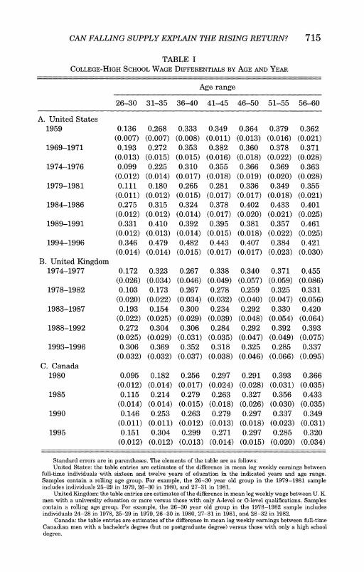
Table I presents our estimates of the "college wage premiums" for five-year age groups, taken at five-year time intervals over our sample period (with the exception of the first observation for the United States).9 Note that to improve the precision of our estimates we have pooled three CPS samples and five GHS sam-

9. Since cohort composition may change over time because of immigration (and mortality), it would be preferable to compute the college wage premium (and the relative supply measures) for native workers only. This is not possible, however, since immigrant status was not identified until recently in the CPS. Fortunately, evidence from the U. S. Census presented in Borjas, Freeman, and Katz [1997] suggests that changes in U. S. educational differentials are similar whether or not immigrants are included.


TABLE I COLLEGE-HIGH SCHOOL WAGE DIFFERENTIALS BY AGE AND YEAR

Age range

26-30 31-35 36-40 41-45 46-50 51-55 56-60

A. United States 1959 0.136 0.268 0.333 0.349 0.364 0.379 0.362

(0.007) (0.007) (0.008) (0.011) (0.013) (0.016) (0.021) 1969-1971 0.193 0.272 0.353 0.382 0.360 0.378 0.371

(0.013) (0.015) (0.015) (0.016) (0.018) (0.022) (0.028) 1974-1976 0.099 0.225 0.310 0.355 0.366 0.369 0.363

(0.012) (0.014) (0.017) (0.018) (0.019) (0.020) (0.028) 1979-1981 0.111 0.180 0.265 0.281 0.336 0.349 0.355

(0.011) (0.012) (0.015) (0.017) (0.017) (0.018) (0.021) 1984-1986 0.275 0.315 0.324 0.378 0.402 0.433 0.401

(0.012) (0.012) (0.014) (0.017) (0.020) (0.021) (0.025) 1989-1991 0.331 0.410 0.392 0.395 0.381 0.357 0.461

(0.012) (0.013) (0.014) (0.015) (0.018) (0.022) (0.025) 1994-1996 0.346 0.479 0.482 0.443 0.407 0.384 0.421

(0.014) (0.014) (0.015) (0.017) (0.017) (0.023) (0.030) B. United Kngdom

1974-1977 0.172 0.323 0.267 0.338 0.340 0.371 0.455 (0.026) (0.034) (0.046) (0.049) (0.057) (0.059) (0.086)

1978-1982 0.103 0.173 0.267 0.278 0.259 0.325 0.331 (0.020) (0.022) (0.034) (0.032) (0.040) (0.047) (0.056)

1983-1987 0.193 0.154 0.300 0.234 0.292 0.330 0.420 (0.022) (0.025) (0.029) (0.039) (0.048) (0.054) (0.064)

1988-1992 0.272 0.304 0.306 0.284 0.292 0.392 0.393 (0.025) (0.029) (0.031) (0.035) (0.047) (0.049) (0.075)

1993-1996 0.306 0.369 0.352 0.318 0.325 0.285 0.337 (0.032) (0.032) (0.037) (0.038) (0.046) (0.066) (0.095)

C. Canada 1980 0.095 0.182 0.256 0.297 0.291 0.393 0.366

(0.012) (0.014) (0.017) (0.024) (0.028) (0.031) (0.035) 1985 0.115 0.214 0.279 0.263 0.327 0.356 0.433

(0.014) (0.014) (0.015) (0.018) (0.026) (0.030) (0.035) 1990 0.146 0.253 0.263 0.279 0.297 0.337 0.349

(0.011) (0.011) (0.012) (0.013) (0.018) (0.023) (0.031) 1995 0.151 0.304 0.299 0.271 0.297 0.285 0.320

(0.012) (0.012) (0.013) (0.014) (0.015) (0.020) (0.034)

Standard errors are in parentheses. The elements of the table are as follows: United States: the table entries are estimates of the difference in mean log weekly earnings between

full-time individuals with sixteen and twelve years of education in the indicated years and age range. Samples contain a rolling age group. For example, the 26-30 year old group in the 1979-1981 sample includes individuals 25-29 in 1979, 26-30 in 1980, and 27-31 in 1981.

United Kingdom: the table entries are estimates of the difference in mean log weekly wage between U. K. men with a university education or more versus those with only A-level or 0-level qualifications. Samples contain a rolling age group. For example, the 26-30 year old group in the 1978-1982 sample includes individuals 24-28 in 1978, 25-29 in 1979, 26-30 in 1980, 27-31 in 1981, and 28-32 in 1982.

Canada: the table entries are estimates of the difference in mean log weekly earnings between full-time Canadian men with a bachelor's degree (but no postgraduate degree) versus those with only a high school degree.

716 QUA!?RTERLY JOURNAL OF ECONOMICS

ples for each time period. Our estimates for the United States are based on differences in mean log average weekly wages between full-time workers with exactly a college degree (i.e., sixteen years of education) and those with exactly a high school degree (i.e., twelve years of education).10 Similarly, our estimates for Canada are based on differences in mean log average weekly wages between full-time workers with a university degree and those with a high school diploma.11 Finally, our estimates for the United Kingdom represent differences in mean log weekly wages between men with a university degree and those with only A-level or 0-level qualifications.'2 The Data Appendix contains more details on the construction of our samples, and the procedures used to obtain the estimated wage gaps.

An important feature of the wage gaps in Table I is that they are based on differences in earnings between individuals of the same age with a college degree or a high school diploma. An advantage of this measure is that it compares individuals who attended elementary and secondary schooling together, and were subject to the same influences on their decision as to whether to attend college. A potential disadvantage is that it ignores any differences in labor market experience between people of the same age who have different levels of schooling. Under the tra- ditional human capital earnings function, for example, one would expect the college-high school earnings gap for people of the same age to rise over the life cycle. Since our econometric models will account for systematic age effects in the structure of the college wage premium, and in view of our interest in cohort-based expla- nations for changes in college wage premiums for different

10. Our use of weekly wages for full-time workers follows Katz and Murphy [1992] and is meant to eliminate variation associated with hours per week or weeks per year. Note that our "college" group excludes those with any postgraduate education. An alternative that is sometimes used in the literature is to compare wages for workers with a college degree or higher with those with a high school degree. As discussed in subsection III.B, however, our main results are not substantially affected by the choice.

11. In Canada the number of years of schooling required to obtain a high school degree varies from eleven to thirteen years depending on the province, while the number of years of schooling required to obtain a bachelor's degree varies from fifteen to seventeen years.

12. We follow Schmitt [19951 in using average weekly wages from the GHS. We pooled people with A-level and at least one 0-level qualification together to form a "high school graduate" group, although only those with A-level qualifications are fully qualified to enter university. This decision was made to increase our sample sizes, since the fraction of people with exactly A-level qualifications is low. Comparisons of wage rates for those with A-level and 0-level qualifications showed that the groups move together very closely over our sample period.


groups, we believe it is appropriate to compare college and high school earnings for men of the same age. As a check on the validity of our conclusions, however, we have conducted many of our analyses using "experience cohorts" (see subsection III.B).

The entries in Table I provide a variety of information on the evolution of the college-high school wage gap. Comparisons down a column of the table show the changing college premium for a specific age group (as in Figure 1). Among 26-30 year olds in the United States, for example, the college wage gap rose somewhat from 1959 to 1970, fell back to its earlier level by the mid-1970s, and then rose sharply throughout the 1980s. For older men in the United States returns also tended to fall in the 1970s and rise in the 1980s, although for groups over age 45 the changes are small.

Comparisons across the rows of Table I reveal the age profile of the college-high school wage gap at a point in time. These profiles are graphed in Figure II and show a surprising degree of similarity across the three countries."3 As shown by the averaged profile for 1959, 1969-1971, and 1974-1976, the college-high school wage gap in the United States in the 1960s and early 1970s was an increasing and slightly concave function of age. Between 1975 and 1980 the entire profile shifted down, with the exception of the youngest age group, whose gap remained constant. By the mid-1980s the gaps for older workers were back to their levels in the mid-1970s, but the gaps for the two youngest age groups were much higher. Moving to 1989-1991, the gaps for the three youngest age groups were substantially higher than those in the mid- 1970s, while those for the older cohorts were not too different. Finally, in 1994-1996, the gaps for the four youngest age groups were well above the levels of the mid-1970s, but the gaps for older age groups were still comparable to those twenty years earlier. A very similar "twisting" of the age profiles is evident for the United Kingdom, although unlike the United States the college wage premiums for older workers in the United Kingdom actually fell in the 1990s. Canada also exhibits a twisting age profile, although the changes are smaller than in the United States or United Kingdom.

The shifting age profiles in Figure II suggest that there are at least two separate forces underlying the evolution of the college wage premium over time. On the one hand, the overall set of wage premiums can rise or fall over time (as they appear to have done

13. The profiles graphed in Figure II are smoothed using a moving average.


A. United States

0.5

1 994-9\s X - -X . , -

00.41~~~~. 8 0-4 - ---- =X.

0.3

z ! 1984 88 -.

19981

o 0.2 -

Average of 1959, 1989-70, 1974-78

0.1 .

26-30 31-35 36-40 41-45 46-50 51-55 56-60 Age Group

B. United Kingdom

0.5 -

(D

CD 0 -4 >

-X~~98---- ......... ~

10.2 -9

- 1978-82

0.1 26-30 31-35 36-40 41-45 46-50 51-55 56-60

C. Canada Age Group

0.2

0.4

0) 0.3

C .~~~~ - ~~1980

1985

0.1iI 26-30 31-35 36-40 41-45 46-50 51-55 56-60

Age Group

FIGURE II Age Profiles of the College-High School Wage Gap


in the United States and the United Kingdom between 1975 and 1980). On the other hand, the relative wage premiums for specific age groups can rise or fall independently of the wage gaps for other groups. In the United States and United Kingdom, the rises in returns for younger workers seem to follow a distinct cohort pattern, with higher returns at each age for the cohorts that entered the U. S. sample after 1980, and for those that entered the U. K. sample after 1985.

B. Cohort Effects in the College Premium?

As noted in Section I, one potential indicator of the presence of age-group specific supply effects in the structure of the college wage gap is the presence of cohort effects. Under the assumption that different age groups are perfectly substitutable, one would expect the college wage premiums for different age groups to rise and fall proportionally over time, with a structure that is fully captured by age and year effects. Under the alternative assumption that different age groups are imperfect substitutes, and that the relative supplies of different age groups are not all trending at the same rate, however, one would expect cohort effects to play some role in explaining the pattern of wage gaps across age groups and over time.

Table II presents a simple investigation of the potential role of cohort effects in explaining the wage gaps shown in Table I. The regression models presented in Table II are of the form

(13) rjt = bj + c tj + dt + eit, where rjt is the estimated college premium for age group j in year t, bj represents a set of age effects (for five-year age bands), ct_j are cohort effects (for five-year birth cohorts), dt are year effects (for time periods five years apart), and ejt represents a combination of sampling error and specification error. Since the sampling variances of the estimated rjt's are known, it is straightforward to construct goodness-of-fit tests for the null hypothesis of no specification error, conditional on the included effects.14

14. Specifically, let r represent the vector of estimated gaps, and let ff represent the true gaps. Given our estimation procedures, r - , is normally distributed with mean 0 and a diagonal covariance matrix E. Let S represent a consistent estimate of S. Under the null that V - f[Cx), where u is a vector of parameters (e.g., cohort, age, and year effects), (r - f(,fT))'S-'(r - f([l)) is asymptotically distributed as x2 with degrees of freedom equal to the number of elements of r minus the number of linearly independent columns of the matrix of derivatives of


TABLE II DECOMPOSITIONS OF COLLEGE-HIGH SCHOOL WAGE DIFFERENTIALS BY AGE AND

YEAR INTO COHORT, AGE, AND TIME EFFECTS

United States United Kingdom Canada

No 10 oldest 10 oldest No 7 oldest 7 oldest No 6 oldest 6 oldest

cohort cohorts coh. eff. cohort cohorts coh. eff. cohort cohorts coh. eff. effects only same effects only same effects only same

Year effects 1970 0.026 0.020 0.020 - - - - - -

(0.021) (0.010) (0.009) 1975 -0.020 -0.024 -0.024 0.000 0.000 0.000 - - -

(0.021) (0.010) (0.009) 1980 -0.049 -0.060 -0.062 -0.077 -0.086 -0.076 0.000 0.000 0.000

(0.019) (0.011) (0.009) (0.026) (0.021) (0.018) 1985 0.058 0.017 0.015 -0.045 -0.057 -0.069 0.020 0.007 -0.004

(0.020) (0.013) (0.010) (0.027) (0.025) (0.021) (0.019) (0.017) (0.013) 1990 0.099 0.022 0.022 0.021 -0.041 -0.037 0.031 -0.011 -0.025

(0.020) (0.015) (0.011) (0.028) (0.028) (0.025) (0.017) (0.018) (0.016) 1995 0.141 0.024 0.034 0.051 -0.060 -0.039 0.043 -0.038 -0.039

(0.021) (0.019) (0.014) (0.030) (0.038) (0.031) (0.017) (0.021) (0.021) Cohort

effects: 1950-1954 - - 0.040 - - -0.009 - - 0.028

(0.011) (0.019) (0.015) 1955-1959 - - 0.124 - - 0.075 - - 0.076

(0.013) (0.025) (0.021) 1960-1964 - - 0.178 - - 0.134 - - 0.133

(0.016) (0.032) (0.027) 1964-1969 - - 0.175 - - 0.162 - - 0.142

(0.024) (0.046) (0.036) Degrees of

freedom 36 26 32 24 14 20 18 9 14

x2 (p-value) 295.01 48.84 51.09 48.31 10.76 15.33 66.06 12.00 20.51 (0.00) (0.00) (0.02) (0.00) (0.70) (0.76) (0.00) (0.21) (0.11)

R2 0.87 0.97 0.98 0.77 0.85 0.92 0.89 0.90 0.97

Standard errors are in parentheses. Models are fit by weighted least squares to the age-group by year college-high school wage gaps shown in Table I. Weights are inverse sampling variances of the estimated wage gaps. All models include age effects. For the United States and the United Kingdom, the years indicated when reporting the estimated year effects are the midpoints of the year intervals shown in Table I. The base (omitted) year is 1959 for the United States, 1975-1977 for the United Kingdom, and 1980 for Canada.

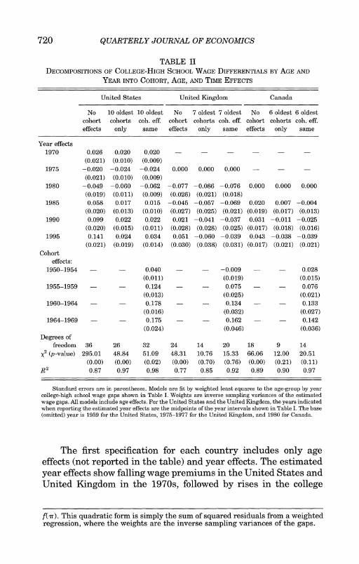
The first specification for each country includes only age effects (not reported in the table) and year effects. The estimated year effects show falling wage premiums in the United States and United Kingdom in the 1970s, followed by rises in the college

f('n-). This quadratic form is simply the sum of squared residuals from a weighted regression, where the weights are the inverse sampling variances of the gaps.


premium for all three countries over the 1980s and 1990s. As might be expected given the patterns in Figure II, the specifications without cohort effects fit very poorly, as indicated by the x2 test statistics at the bottom of the table. The second model for each country reports the same specification, fit to data for only the oldest cohorts in each country (specifically, for cohorts born before 1950). When the models are limited to these older cohorts, the fits improve substantially, and the estimated patterns of year effects are also quite different. In the United States the year effects for the oldest cohorts show a larger decline in the college premium over the 1970s, and a much smaller rise during the 1980s and 1990s. For the United Kingdom, the year effects show a decline in the college premium from 1975 to 1980 and relative stability thereafter. For Canada the year effects show a small decline over the 1980s. Finally, the third model for each country is fit to data for all available cohorts, but includes unrestricted cohort effects for those born after 1950. These models fit relatively well, and yield a set of year effects that are very similar to the year effects from the second specification. Interestingly, for all three countries most of the apparent rise in relative returns to college over the 1980s and 1990s is attributable to the labor market entry of cohorts with permanently higher returns to college, rather than to a general rise in returns for all age groups. These results confirm the impression conveyed by the age profiles in Figure II, and suggest that cohorts who entered the labor market after the mid-1970s had a very different structure of college wage premiums than earlier cohorts.

C. Relative Supplies

We turn next to an overview of our estimates of the relative supplies of college-educated labor by age group and year. Follow- ing Katz and Murphy [19921, we estimate relative supplies from a very broad sample of workers in each year (we include all wage and salary and self-employed workers age 20 to 65). To account for differences in the effective supply of labor by different groups, we count the number of annual hours supplied by each worker and weight these hours by the average wage (over all periods) of his or her education group. We define the amount of "high-school labor" of age group j in year t (Hjt) as the total annual hours worked by high school graduates in that age range, plus the total hours of high school dropouts (weighted by their wage relative to high school graduates), plus a share of the hours worked by


workers with some college.15 This share is the implicit "high school weight" used to express the wages of workers with some college as a weighted mean of high school and college wages. (For example, the share is equal to two-thirds if workers with some college earn 10 percent more than high school workers and 20 percent less than workers with exactly a college degree). Simi- larly, the amount of "college labor" of age group j in year t (Ct) is defined as the total annual hours worked by college graduates in age group j, plus the total hours of those with over sixteen years of education (weighted by their wage relative to college graduates), plus the appropriate share of the hours worked by workers with some college.

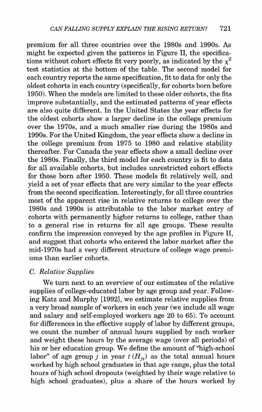
Figure III shows the evolution of our estimates of the log of the relative fraction of college versus high school labor in two representative age groups: 26-30 year olds (in Panel A) and 46-50 year olds (in Panel B). The graphs indicate an important difference between the trends in the relative supply of college labor for younger versus older workers. For older workers, relative supplies trended upward fairly steadily over our entire sample period. For younger workers, however, relative supplies stagnated throughout the 1980s and 1990s.

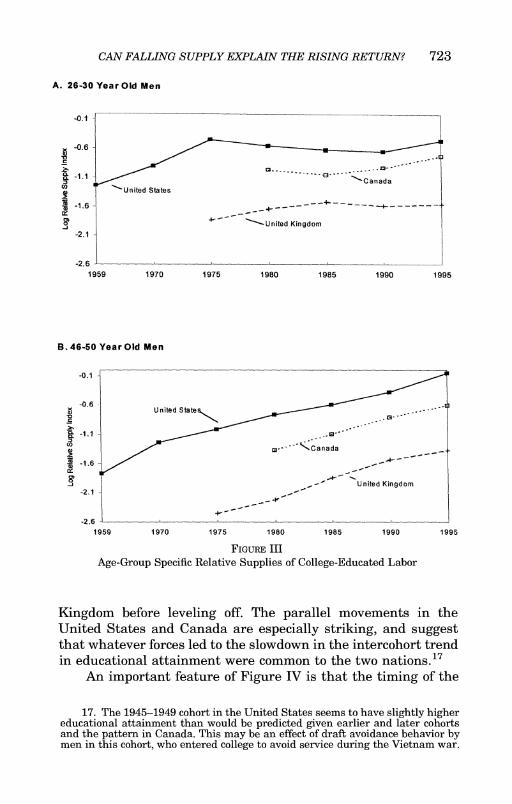
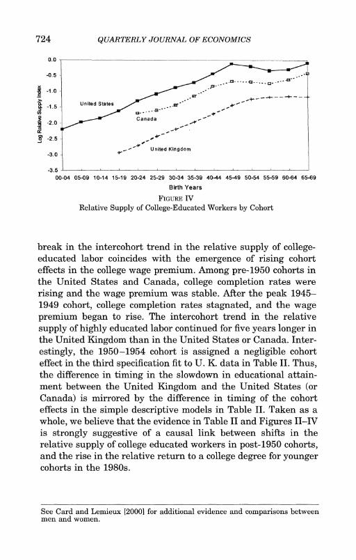
To further investigate the trends in Figure III, we fit models with cohort and age effects to data on the relative fraction of college workers by age group and year for each country. Consis- tent with the hypothesis that educational attainment of a cohort is fixed over time (apart from a common aging effect), these models fit very well, with R2 coefficients exceeding 98 percent. The estimated cohort effects for the three countries are plotted in Figure IV.16 In all three countries there was a positive intercohort trend in the relative fraction of college educated workers for cohorts born before 1950. After the 1945-1949 cohort educational attainments actually declined somewhat in the United States and Canada, but continued to rise for five more years in the United

15. In the United Kingdom an important fraction of workers report vocational training as their highest level of education. Since workers with the lowest level of vocational training earn less than high school graduates ("O" or "A" level degrees), we classify them as "high school" and weight them by their average wage. Workers with higher levels of vocational training have wages in between those of high school and college graduates. We treat them like the "some college" group in the United States (and divide them between high school and college). Workers with vocational training in Canada are also treated like the "some college" group since their wages are in between those of high school and college graduates.

16. The cohort effects are standardized to age 41-45.


A. 26?30 Year Old Men

-0.1I

X. -0.6

.......... .l .. , - - - ' - '

CO) X F nited States

g -1.6

: + ~-V-United Kingdom -2.1

-2.6 - .

1959 1970 1975 1980 1985 1990 1995

B. 46-50 Year Old Men

-0.1I

IXV -0.6

. Unitd States

a -1.1 X+-

<-~ Canada-

.~-1.6

2.1 _- United Kingdom -2.1

-2.6 1959 1970 1975 1980 1985 1990 1995

FIGURE III

Age-Group Specific Relative Supplies of College-Educated Labor

Kingdom before leveling off. The parallel movements in the United States and Canada are especially striking, and suggest that whatever forces led to the slowdown in the intercohort trend in educational attainment were common to the two nations.17

An important feature of Figure IV is that the timing of the

17. The 1945-1949 cohort in the United States seems to have slightly higher educational attainment than would be predicted given earlier and later cohorts and the pattern in Canada. This may be an effect of draft avoidance behavior by men in this cohort, who entered college to avoid service during the Vietnam war.


o.o

0 15j=.0... a - ' . . __ __ t -- + l _ _ __ __ __ _

-0.5

-1.0 - C e-r

-1. United States -r= r a, 'a- ---

Canada tg -2.0 -14

-2.5

-3.- _- United Kingdom

-3.5 g t , , _ S | , ; 00-04 05-09 10-14 15-19 20-24 25-29 30-34 35-39 40-44 45-49 50-54 55-59 60-64 65-69

Birth Years

FIGURE IV Relative Supply of College-Educated Workers by Cohort

break in the intercohort trend in the relative supply of college- educated labor coincides with the emergence of rising cohort effects in the college wage premium. Among pre-1950 cohorts in the United States and Canada, college completion rates were rising and the wage premium was stable. After the peak 1945- 1949 cohort, college completion rates stagnated, and the wage premium began to rise. The intercohort trend in the relative supply of highly educated labor continued for five years longer in the United Kingdom than in the United States or Canada. Inter- estingly, the 1950-1954 cohort is assigned a negligible cohort effect in the third specification fit to U. K. data in Table II. Thus, the difference in timing in the slowdown in educational attainment between the United Kingdom and the United States (or Canada) is mirrored by the difference in timing of the cohort effects in the simple descriptive models in Table II. Taken as a whole, we believe that the evidence in Table II and Figures II-IV is strongly suggestive of a causal link between shifts in the relative supply of college educated workers in post-1950 cohorts, and the rise in the relative return to a college degree for younger cohorts in the 1980s.

See Card and Lemieux [20001 for additional evidence and comparisons between men and women.


TABLE III ESTIMATED MODELS FOR THE COLLEGE-HIGH SCHOOL WAGE GAP,

By COHORT AND YEAR

United States United Kingdom Canada

(1) (2) (3) (4) (5) (6)

Age-group specific -0.203 -0.265 -0.233 -0.261 -0.165 -0.161 relative supply (0.019) (0.026) (0.058) (0.071) (0.042) (0.040)

Trend 0.012 0.013 - 0.006 (0.001) (0.003) (0.001)

Year effects: 1970 0.104 -

(0.012) 1975 0.124 0.0 -

(0.017) 1980 0.129 -0.032 - 0.0

(0.019) (0.023) 1985 0.255 0.060 - 0.029

(0.020) (0.034) (0.014) 1990 0.301 0.149 - 0.054

(0.021) (0.039) (0.014) 1995 0.365 0.199 - 0.089

(0.023) (0.044) (0.017) Degrees of freedom 35 40 23 26 17 19 x2 (p-value) 66.62 209.34 25.78 52.03 35.00 35.68

(0.00) (0.00) (0.31) (0.00) (0.01) (0.01) R 2 0.97 0.91 0.86 0.72 0.94 0.94

Standard errors are in parentheses. Models are fit by weighted least squares to the age-group by year college-high school wage gaps shown in Table I. Weights are inverse sampling variances of the estimated wage gaps. All models include age effects. For the United States and the United Kingdom, the years indicated when reporting the estimated year effects are the midpoints of the year intervals shown in Table I.

III. THE EFFECT OF COHORT-SPECIFIC SUPPLIES ON THE COLLEGE WAGE PREMIUM

A. Basic Estimates

We now turn to the estimation of the effects of the relative supply of college-educated workers on the college-high school wage gap. Table III presents a set of models for the first stage of our two-step estimation procedure. The first specification for each country regresses the age-group specific relative wage premium on age and year effects, and the age-group specific relative supply index. The estimated effects of the relative supply index are very similar across countries (in the range of -0.23 to -0.17) and are


fairly precise. The estimates imply an elasticity of substitution between different age groups in the range of 4 to 6. Moreover, for the United Kingdom and Canada the models provide a relatively good fit. The estimated year effects, which absorb both the relative technology shock (log (0Ct10ht)) and any effect of changing aggregate supply ([(1/CTA) - (1IcrE)] log (CtlHt)) show a pattern of steeply rising relative returns in all three countries. The second specification for each country takes out the unrestricted year effects and replaces them with a linear trend. Although the models with a linear trend term do not fit the data as well as the models with unrestricted year effects, the estimates of the critical coefficient relating age-group specific relative supplies to age- group specific college wage premiums remain relatively unchanged.

Table IV presents estimates of the second-stage models (based on equation (8b)) that include both age-group specific relative supplies of college labor, and the aggregate relative supply index. The first specification for each country ignores imperfect substitutability across age groups in the construction of the aggregate supply index, and simply uses the weighted hours index developed by Katz and Murphy [1992], including both men and women in the construction of the index.18 The relative technology shock variable (log (0ctlOht)) is assumed to follow a linear trend. The results from this specification are very similar for the United States and United Kingdom, and suggest that the elasticity of substitution between college and high school labor equivalents is in the range of 2 to 2.5.19 For Canada, on the other hand, the aggregate supply variable has no significant effect. It is also interesting to note that the estimates of 1/AA from the second- stage procedure are very close to the first-stage estimates. The second specification for each country uses an aggregate relative supply index that assumes imperfect substitution across age groups.20 Perhaps because the estimated elasticities of substitution across age groups are relatively high, results based on this

18. We obtain similar results when the index is constructed using men only. 19. By comparison, Katz and Murphy [1992] report an estimate of 1lcE equal

to 0.71 (for men and women), implying that SE = 1.4. Their results are very similar, however, to those we obtain when we also use men and women (see Table VI).

20. This supply index includes men only. We present results for men and women combined in the next section. The estimates of 1hA are taken from the first specification for each country reported in Table III.


0 cl ~o t o C. LO co O )O o . N 00 O 00A

I

s I , I v Z H

~~~CO: > b02

Q0 di CY cs

cz 44 C. ,o,o to I X,. >o ,

00~~~~~~~~~~~~~~~~~ ~ '-00 4

0 66 oo cSoo S

O~~~~~~~~~~~~~O~r . CYD C2 LO O O O O 00 1 - I0j 0

r Hz<- ~oo oi) oo

00I000 00 0 C00i000

q n e > O > H H m m z Q tq c

b.0

00 C.0 ~~~~~~~~~~~~~~~~~~~~~~~~00 L /O Ol O OOOO /bO O-

' N'0 0 0 -00 p

00 t- C.0 Q0 ~~~~~~~~~~~00

00

000 6

D~~~~~~~C r-qriC Xr- cq LO O Q0 CdO W

o c 0 0 o o O I

co000 0

0000 00 000L -1C 4 4

c a)

~~~~~~~~~~~~~m CD I'd

0! n4O~4j 00 Ot'- oo

< nON~~~~0 C9 t-n

0 -O -4 O0 ?O- 0 10 i-400 o O

D~~~~~~~c)C tg

:~0100000 000 %000 d

666ooo 66 00~~~mC66 s.

o 0)

012~~~~~~~~~~~~~~~~-

Q 000 00 11 D m N O e 0N 00 % nT > 00 c

W~~~~I- "- 0000"- 0) O0t

00

0 C9C9>N C~0.~l ooo

a)0

0 on0U

-4 Q 00~~~~~~~~~~~00

On a) EE 2 E-) 02 "0 0)0


0-

-0.5-. Q 05

13)

2r 25

1955 1960 1965 1970 1975 1980 1985 1990 1995

ME US --v UK Canada

FIGURE V Aggregate Relative Supply Index for Men

index are very similar to results based on a simpler aggregate index that assumes perfect substitutability.

Although the estimates of 1/cA from the second-stage procedure are very close to the first-stage estimates shown in Table III, the fit of the second-stage models is relatively poor, especially for the United States and United Kingdom. Inspection of the year effects in the unrestricted models in columns (1) and (3) of Table III hints at the source of the difficulty: controlling for age-group relative supplies and age effects, aggregate returns to college in the United States increased by about one percentage point a year between 1959 and 1975, stagnated between 1975 and 1980, and jumped by twelve percentage points between 1980 and 1985 before returning to a steady growth rate of 1 percent a year after 1985. In the United Kingdom (column (3) of Table III), aggregate returns to college dropped between 1975 and 1980 before increasing sharply between 1980 and 1985. Thus, in both countries, returns to college were sharply lower in 1980 than would be predicted by a smooth upward trend, controlling for age-group- specific relative supplies of college labor. Unless the aggregate supply variable exhibits a sharp surge in 1980 relative to its trend, the second-stage model cannot account for the relative dip in returns to college in 1980.

Figure V plots the aggregate relative supply indexes for the three countries used in the second-stage models. While the U. S. aggregate supply index grew at a relatively faster pace between 1970 and 1975, the growth between 1975 and 1980 is close to the


average growth rate from 1959 to 1995. In the United Kingdom the relative supply index grew relatively quickly between 1975 and 1980, but even more quickly between 1980 and 1985. Thus, there is no indication of an unusual surge in the aggregate supply of college labor in the late 1970s in either country. Based on this evidence, we conclude that shifts in the aggregate supply of college workers cannot fully account for the dip in returns to college in 1980 in the United States and the United Kingdom, explaining some of the poor fit of the models in columns (2) and (5) of Table IV.

The third set of models in Table IV (columns (3), (6), and (9)) addresses the goodness of fit of the 1980 data more directly by including a dummy variable for this year. The addition of a 1980 year effect improves the fit of the U. S. model, but also reduces the estimated effect of the aggregate supply index by 30 percent. For the United Kingdom the model with a 1980 year effect passes the goodness-of-fit test at standard significance levels and yields a slightly larger estimate of the effect of the aggregate supply index. Overall, however, the estimated elasticities of substitution between age and education groups are surprisingly stable across countries and across specifications, with the exception of the estimate of l/crE for Canada, which is very imprecisely estimated.21

B. Alternative Specifications

We have investigated the robustness of the findings in Tables III and IV to several specification choices. For the sake of brevity, we present the results of these specification checks only for the United States.

A first specification issue is the definition of the education groups used to compute the college-high school wage gap. We believe that the earnings gap between workers with exactly a college degree and those with exactly a high school degree is a relatively accurate gauge of the college premium because these two groups have a fixed four-year difference in schooling. An alternative measure that is sometimes used in the literature is the wage gap between workers with sixteen or more years of education and those with exactly a high school degree. A potential advantage of this alternative measure is that it includes all

21. Since aggregate relative supply essentially follows a linear trend in Canada (see Figure V), its effect cannot separately be identified from the effect of the linear time trend. The large standard errors reflect this identification problem.


college graduates, and not just those who obtained exactly a bachelor's degree. A disadvantage is that the mean level of schooling among those with sixteen or more years of education varies over time: this introduces an added source of variation in the measured college wage gap.22

An even broader measure of the college-high school wage gap is obtained by computing average wages for standardized units of "college labor" and "high school labor." In subsection II.C we estimated the supplies of the two education groups by combining weighted sums of the hours worked by different education groups. Corresponding wage indexes can be obtained by dividing the total "high school wage bill" (the earnings of high school graduates, high school dropouts, and an appropriate fraction of workers with some college) by the total number of units of "high school labor," and the total college wage bill by the number of units of "college labor."

Columns (1) and (2) of Table V show second-stage estimation results for our models using these alternative measures of the college high-school wage gap. The estimated effects of age group relative supplies are somewhat smaller than when we use the narrower definition based on exactly college and exactly high school workers (see Table IV). In all cases, however, the estimated effect is negative and highly significant.

A second specification issue is the choice of sample period. Since our U. S. sample period is so much longer, the results may not be comparable to those based on shorter sample periods for the United Kingdom and Canada. We investigate this issue in columns (3) and (4) of Table V, which present some alternative specifications fit to U. S. data for 1975-1995. Column (3) shows estimates for the base specification (column (2) of Table IV) re- stricted to the 1975-1995 period. The estimated effect of age- group specific relative supplies is similar in the two sample periods (-0.209 for 1959-1995 versus -0.237 for 1975-1995).

Limiting the analysis to the 1975-1995 has another advantage. Starting with the March 1976 survey (earnings for 1975), the CPS collected information on weeks worked and usual hours per week during the previous year. This information can be used

22. See Card and Lemieux [1999] for evidence that the fraction of college graduates who hold a postgraduate degree has changed dramatically over time. For example, 41 percent of college graduates age 26 to 30 had postgraduate training in 1975. By 1995 this fraction had fallen to 22 percent for the same age group.


TABLE V ROBUSTNESS OF THE RESULTS TO ALTERNATrVE MEASURES OF THE COLLEGE-HIGH

SCHOOL WAGE GAP, UNITED STATES

Wage gap by age group

1959-1995 1975-1995 Wage gap by

AWE of Experience Coll + Coll "labor" FT Av. hourly Group, vs. HS vs. HS "labor" wkrs earnings 1959-1995

(1) (2) (3) (4) (5)

Age-group rel. supply -0.157 -0.125 -0.237 -0.218 -0.107

(0.023) (0.020) (0.033) (0.035) (0.048) Aggregate supply

index -0.562 -0.426 -0.355 -0.400 -0.618 (0.056) (0.042) (0.135) (0.146) (0.103)

Trend 0.026 0.020 0.017 0.017 0.024 (0.002) (0.002) (0.004) (0.004) (0.004)

Degrees of freedom 39 39 25 25 39 R2 0.96 0.95 0.93 0.91 0.73

Standard errors are in parentheses. Models are fit by weighted least squares. In column (4) the wage gap is measured using average hourly earnings for all workers; in all other models, the wage gap is measured using average weekly earnings for full-time workers. The wage gap measure used in column (1) is the log wage difference between workers with a college or a postgraduate degree, and workers with exactly a high school degree. The wage gap measure used in column (2) is obtained from the ratio of the average wage of all "college" workers (wage bill of college workers divided by the number of units of college labor) to the wage of all "high school" workers (see the text for more detail). The wage gap used in columns (3) and (4) is the log wage difference between workers with exactly a college degree and workers with exactly a high school degree. The wage gaps in column (5) represent the wage difference between college and high school workers with the same level of potential labor market experience. Only workers with 3 to 37 years of experience (grouped in five-year categories) are used in the estimation. In all other columns the wage gaps represent the wage difference between college and high school workers of the same age. Seven age groups (26-30 to 56-60) are used in the estimation (seven experience groups in column (5)).

to compute average hourly earnings for all workers (not just full-time workers), providing a broader wage index. Column (4) report estimated models fit to the college high school wage gaps in hourly wages for all male workers. A comparison with the results in column (4) shows very similar estimates of the substitution elasticities.

A third specification issue is the use of age, rather than potential labor market experience, to define cohorts. To investigate the effect of this choice, we reestimated the college-high school wage gaps by experience cohort, assuming that college-


educated men enter the labor market on average about five years later than men with only a high school degree.23

Column (5) reports estimates of second-step models in which the dependent variable is the college-high school wage gap for workers in different experience groups (relative supplies are defined accordingly) for workers with 3 to 37 years of potential experience (ages 21 to 55 for high school graduates and 26 to 60 for college graduates). The estimated effect of experience-group specific supplies of college-educated labor is smaller and less precise than for corresponding age-group models. It is not statistically different, however, from the "typical" estimate of -0.2 obtained with the age models.24 Overall, the specification checks in Table V give us reasonable confidence that the elasticity of substitution across age groups is in the range from 4 to 6.

Up to this point, we have focused exclusively on the evolution of the college wage gap for men. On the one hand, we believe that this focus is appropriate, given intercohort changes in female labor supply that have presumably affected the age profiles of earnings for women in different education groups over the past 30 years. In the standard human capital earnings model, the college- high school wage gap at a given age is equal to the true college premium plus the effect of the difference in labor market experience between high school and college graduates of the same age. If women in younger cohorts accumulate more actual experience per year of potential experience than older cohorts, this will increase the measured college-high school wage even if the true college premium is fixed. Secular changes in the age profile of the college-high school wage gap may, therefore, be contaminated by these composition effects.

On the other hand, our focus on men only is only valid if men and women with similar age and education are not substitutes in production. This is clearly a very strong assumption that war- rants further investigation, especially in light of the relative rise in the educational attainments of women over the 1980s. A natural check on the robustness of the results is to reestimate the

23. Thus, college-educated men age 26-30 are in the same experience cohort as high-school-educated men age 21-25. The assumption of a five-year gap was made mainly for convenience, to correspond to the five-year observation intervals we use throughout this paper.

24. When the model for experience groups is estimated for the 1975-1995 period only (not reported in the table), the estimated inverse substitution elasticity is -0.232 (standard error of 0.094), which is very similar to the estimates from the same period for age groups.


TABLE VI MODELS FOR THE COLLEGE-HIGH SCHOOL WAGE GAP FOR MEN AND WOMEN IN THE

UNITED STATES, By COHORT AND YEAR

(1) (2) (3) (4) (5)

Age-group specific relative - -0.221 -0.230 -0.223 supply (0.020) (0.031) (0.022)

Aggregate supply index - - - -0.865 -0.628 (men and women) (0.091) (0.074)

Time trend - - 0.035 0.027 (0.003) 0.003

Year effects: 1970 0.037 0.033 0.034 - -

(0.019) (0.009) (0.009) 1975 -0.009 -0.010 -0.001 -

(0.019) (0.008) (0.009) 1980 -0.035 -0.045 -0.028 -0.057

(0.017) (0.008) (0.008) (0.009) 1985 0.061 0.025 0.058

(0.017) (0.009) (0.008) 1990 0.124 0.058 0.112 -

(0.017) (0.009) (0.008) 1995 0.174 0.087 0.161 -

(0.018) (0.011) (0.009) Cohort effects:

1950-1954 0.033 (0.009)

1955-1959 0.106 -

(0.011) 1960-1964 0.145 - - -

(0.013) 1965-1969 - 0.133 -

(0.019) Degrees of freedom 36 32 35 39 38 x2 (p-value) 331.80 56.31 73.91 194.42 93.46

(0.00) (0.01) (0.00) (0.00) (0.00) R 2 0.89 0.98 0.98 0.94 0.97

Standard errors are in parentheses. Model are fit by weighted least squares to the age-group by year college-high school wage gaps. Weights are inverse sampling variances of the estimates wage gaps. All models include age effects.

models under the polar assumption that men and women with similar age and education are perfect substitutes in production.

Table VI presents the results from a few key models in which both male and female workers are used to construct the college-


high school wage gaps and the relative supply measures.25 Col- umn (1) presents a model that includes only age and year effects. As in the case for a similar specification fit to data for men only (column (1) of Table II), the fit of this model is poor. The fit improves substantially when cohort dummies (for post-1950 cohorts) are included in column (2). The addition of these cohort dummies also reduces by about one-half the estimated upward trend in the average college-high school wage gap captured by the year effects.

The results from models that include relative supply vari- ables are reported in columns (3) to (5).26 The estimated effect of the age-group specific relative supply variable is stable at around -0.22 in all three models, very close to the estimated effects for men only. The only substantial difference between these results and those for men is that the effect of the aggregate relative supply index is larger for men and women (in the -0.6 to -0.9 range) than for men only (range of -0.3 to -0.5 in Table IV). The results for a combined sample of men and women suggest an elasticity of substitution between college and high school graduates in the range of 1.1 to 1.6, which is similar to the estimate reported by Katz and Murphy [1992] who also pool men and women together.

We have performed several other specification checks that are not reported in the tables for the sake of brevity. In one set of results we examined the effect of changing unionization on measured wage differentials between college and high school workers.27 Historically, trade unions have exerted an important influ- ence on the wage structure of adult male workers.28 Over the past two decades union coverage rates-especially for younger, less well-educated men-have fallen sharply in the United States (see, e.g., Card [1998]). Since union coverage is typically associated with a 15-20 percent wage premium for less well-educated men, recent shifts in unionization may have raised the college- high school wage gap among younger workers.

25. Katz and Murphy [1992] also rely implicitly on the assumption of perfect substitution to pool men and women together in their analysis of the effect of aggregate relative supply on the college-high school wage gap.

26. In all three models, age-group specific relative supply is expressed in deviations relative to aggregate relative supply, as in equation (8b).

27. See Fortin and Lemieux [1997] for a review of the effect of labor market institutions on the wage structure.

28. Another potentially important labor market institution-the minimum wage-has relatively little impact on male workers over age 25 with at least twelve years of education.


Consistent with this prediction, we find that the college-high school differential in union coverage has a positive effect on the college-high school wage gap (see Card and Lemieux [19991 for more details). We also find, however, that including this variable in specifications like those in Table IV only marginally changes the estimated effect of age-group specific relative supplies on the college-high school wage gap.29

C. Freeing Up the Elasticity of Substitution by Education Groups A limitation of the model of subsection II.A is that the elas-

ticity of substitution across age groups (UA) is assumed to be the same for college and high school workers. The model is easily generalized by introducing separate elasticities of substitution crAH and OrAc for high school and college workers, respectively. Under the assumption that relative wages are equated to relative marginal products, equations (5) and (6) can be used to derive a pair of wage determination equations:

(14a) log (Wyhl) = log (Oht) + log (ji)

[((JH) (JE)|g ( ) ((AH)log (Hjt) + eht [(1~ 1 ~jlog (Ht) - jt

1

LUOAH/ (E I] AH / jt

and

(14b) log (wjt) = log (O,t) + log (fl)

+(1A - log (C) log (Cjt) + ejc, L\AC/ \UE/Jog \UAcI rAC

where H' and C' are the same labor aggregates as in equations (1) and (2) except that the parameter -q is now specific to each education group, and e4?t and eit are error terms that include a function of Pt plus any specification or sampling errors.

Equations (14a) and (14b) can be estimated separately to test whether the effect of the age-group specific supplies (Hjt and Cjt) are the same for college and high school graduates. The test is

29. Interestingly, the same pattern of de-unionization among young and less-educated men holds in Canada, despite the fact that the overall unionization rate has declined much more slowly than in the United States (see DiNardo and Lemieux [19971 and Riddell [1993]). Because of data limitations, however, it is difficult to estimate precisely the effect of changes in union coverage on the college-high school wage gap in Canada.


TABLE VII MODELS WITH DIFFERENT ELASTICITIES OF SUBSTITUTION BY EDUCATION LEVEL,

UNITED STATES

Fixed Fixed OLS GLS effects effects

Estimation method: (1) (2) (3) (4)

Effect of HS supply on HS -0.183 -0.178 -0.211 -0.201 wages (0.030) (0.026) (0.028) (0.027)

Effect of college supply on -0.119 -0.176 -0.210 -0.204 college wages (0.035) (0.030) (0.030) (0.023)

Weighted by inverse sample No No No Yes variance of college-hs wage gap

Standard errors are in parentheses. All the models are estimated for 98 age x year X education groups from 1959 to 1995 (seven age groups, 26-30 to 56-60, seven years, 1959 to 1995, and two education groups, high school and college). The dependent variable is the mean log average weekly wage for full-time workers in the group. Only workers with exactly a high school degree or exactly a college degree are used to construct mean wages. All models also include a set of age and year effects fully interacted with a dummy variable for college status. In the OLS estimates reported in column (1) the regression error is assumed to be uncorrelated across age x year x college groups. In column (2) a possible correlation is introduced between the error terms of age x year groups with a high school and a college degree. In columns (3) and (4) a full set of age x year dummies is included in the models.

easily implemented by noting that age and year effects absorb all the terms in these equations except the final ones. OLS estimates of equations (14a) and (14b) based on this idea are reported in column (1) of Table VII. As expected, age-group specific supplies have a negative and significant effect on the level of both high school and college wages. The inverse elasticity of substitution across age groups is smaller for college than high school graduates (implying a higher degree of substitution across age groups for more highly educated workers), although the difference is not statistically significant.

More efficient estimates are obtained by allowing for a possible correlation between the error terms e t and e t. The resulting generalized least squares (GLS) estimates are reported in column (2) of Table VII. As in column (1), the estimates are negative and significant. Unlike the results in column (1), however, the implied elasticities are quite close, and both in the 5-6 range. Interest- ingly, the magnitude of these estimates is fairly similar to estimates obtained by Welch [1979] who finds that the effect of age-group specific supplies on wages is -0.10 and -0.22 for high

CAN FALLING SUPPLY EXPLAMN THE RISING RETURN? 737

school and college graduates, respectively.30 More recent work by Juhn, Kim, and Vella [1999] also finds that the age-group specific relative supply of college-educated workers has a negative effect on college wages.31

Column (3) presents the results from another specification that includes age x year fixed effects. These are introduced to control for unobserved factors that are common to both high school and college graduates in the same year, and may be correlated with the age-specific supplies. For example, cohorts born after 1950 may have experienced unusually low levels of earnings even after controlling for other factors. If these cohort effects in the level of wages are correlated with supplies, the OLS and GLS estimates will be inconsistent.

The fixed effects estimates of the inverse substitution elasticity reported in column (3) are almost identical for college and high school graduates, with implied elasticities of substitution around 5. Note that these estimates are equivalent to the estimates that would be obtained by running OLS on the difference between equations (14a) and (14b):

(15) rjt = bj + dt - (IIUAC) log (Cjt) + (IIUAH) log (Hjt) + eJt -ejt

where the terms other than age-group specific supplies are absorbed by the age (bj) and year (dt) dummies. The models that we reported in subsections IIL.A and IIL.B can, therefore, be inter- preted as fixed effects models for the wage levels. In our earlier estimates we used the inverse sampling variances of the estimated returns as weights. When we use a similar weighting procedure for a model that allows different coefficients on the relative supplies of college and high school labor we obtain the results reported in column (4) of Table VII. Once again, the

30. These estimates are the "persistent" effects (Welch finds larger effects for entry cohorts) of cohort size on weekly earnings of white males, controlling for part-time status. See Table 8 in Welch [1979].

31. It is difficult to compare our estimated elasticities with those of Juhn, Kim, and Vella [1999] since, for each cohort, they include both the relative supply of college workers and the share of the population that has a college degree in their wage equations. The latter variable is included in an attempt to control for changes in the "quality" of college workers induced by changes in the proportion of the population that holds a college degree. In a related paper Rosenbaum [2000] concludes that part of the increase in the college premium is attributable to changes in the skill composition of educational groups across cohorts. These composition effects cannot, however, explain why the college premium increased faster for younger than older workers, which is the main focus of our paper (see Appendix Tables 1 and 2 in Rosenbaum [2000]).


estimated substitution effects are almost identical for college and high school workers. The results also show that weighting has little effect on our estimates. In summary, we believe that there is compelling evidence that the elasticity of substitution across age groups is about 5 for both college and high school workers.

IV. WHAT CAUSED THE SLOWDOWN IN THE INTERCOHORT TREND IN

EDUCATIONAL ATTAINMENT?

An important question raised by our findings is what caused the slowdown in the intercohort trend in college graduation rates that seems to have affected all three countries in our analysis? One possible explanation that is suggested by the timing of the slowdown is that cohorts at the peak of the baby boom were "crowded out" of college. In the United States, for example, the 1950-1954 cohort was about 13 percent bigger than the 1945-1949 cohort, while the 1955- 1959 cohort was 27 percent bigger. These comparisons suggest that the U. S. college system would have had to continue expanding in the early 1970s if the peak baby boom cohorts were to attend college at higher rates than the 1945-1949 cohort (and maintain the rising trend set by earlier cohorts). Moreover, female college attendance rates were rising, leading to even greater competition for college slots in the 1970s. A potentially attractive feature of the "cohort crowding" hypothesis is that the United States, Canada, and the United Kingdom all experienced baby booms in the 1950s-thus, this hypothesis may be able to explain the similarity of the slow- downs in all three countries.

The baby booms were not exactly the same, however, in the three countries. In particular, although the patterns of births were very similar in the United States and Canada, the baby boom peaked about five years later in the United Kingdom.32 Interest- ingly, the slowdown in educational attainment also occurred five years later in the United Kingdom (see Figure IV). The coincidence of timing between the peak of the baby boom and the break in the intercohort trend in educational attainment highlights the potential role of cohort size as an explanation for intercohort trends in relative supply.

We have explored this explanation in more detail for the United States in Card and Lemieux [2000]. Using interstate

32. The post-1950 baby boom peaked in the late 1950s in Canada and the United States, but only in 1964 in the United Kingdom.


variation in the growth rates of the population of different age groups, we find that the cohort size effects can explain as much as one-quarter of the intercohort slowdown in educational attainment. We have also explored the role of other factors linked to family background such as intercohort changes in parents' education but found that these factors cannot explain much of the slowdown.

Another possible explanation for the slowdown in the educational attainment of post-1950 U. S. cohorts is that the return to college was low in the 1970s when these cohorts had to decide whether to attend college (see Freeman [1976]). The problem with this explanation is that, in light of the extremely high returns to college of the late 1980s, college attendance rates should have increased dramatically for cohorts born in the late 1960s. Figure IV shows, however, that the education attainment for this cohort is the same as for men born twenty years earlier.33 The prolonged stagnation in the educational attainment of U. S. men remains a puzzle in light of the dramatic rise in returns to college for young men in the 1980s and 1990s.

V. CONCLUDING COMMENTS

This paper is motivated by the observation that the college- high school wage gaps of different age groups have not moved together over the past two decades. In particular, the college premium for younger workers in the United States and the United Kingdom has risen substantially, while the premium for older workers is about the same today as it was in the mid-1970s. The college-high school wage gap for young workers did not rise as dramatically in Canada, but the gap for older Canadian men declined substantially over the 1980s. In all three countries the relative age structure of the college premium has thus shifted in the same direction.

Using a model that incorporates imperfect substitution between similarly educated workers in different age groups, we argue that this shifting structure can be largely explained by a combination of cohort-specific relative supplies of college-equivalent labor and steady rises in the relative productivity of college workers (i.e., a constant rate of skill-biased technical change).

33. In Card and Lemieux [2000] we show that college entry rates among male high school seniors are about the same today as in the late 1960s.


Within this framework, the increase in the college-high school wage gap over the past two decades is attributable to steadily rising relative demand for college-educated labor, coupled with a dramatic slowdown in the rate of growth of the relative supply of college-educated workers. This very simple model provides a unifying explanation for the observed changes in the college wage premium in all three countries. Moreover, estimates of the underlying technology parameters for the three countries are gen- erally similar. The success of this explanation is remarkable in view of the very different levels of educational attainment in the three countries, and the fact that the average college wage premium has trended differently in the United States, Canada, and the United Kingdom.

A key issue for future research is to understand the sources of the slowdown in the intercohort trend in educational attainment that has affected the post-1950 cohorts in all three countries. Our results suggest that if cohorts born after 1950 had been able to maintain the trend set by earlier cohorts, educational levels would be higher today, and the college wage premium would be lower.

DATA APPENDIX

A. Wage Data

United States

The wage gaps in Table I are based on samples of men in the 1960 Census and the March CPS. The 1959 data are drawn from the 1960 Census; the 1969-1971 data are drawn from the March 1970- 1972 CPS; the 1974-1976 data are drawn from the March 1975- 1977 CPS; the 1979-1981 data are drawn from the March 1980- 1982 CPS; the 1984-1986 data are drawn from the 1985-1987 CPS; the 1989-1991 data are drawn from the March 1990-1992 CPS; and the 1994-1996 data are drawn from the 1995-1997 CPS. The CPS samples for "year t" (t = 1970,1975,1980,1985,1990,1995) include men who were age 26-60 in t, plus men who were 25 to 59 in t - 1; plus men who were 27 to 61 in t + 1. Weekly wages of full-time workers are formed by dividing annual wage and salary earnings by an imputed measure of weeks worked during the previous year for individuals who worked full-time in the week prior to the survey (or census) week.


This choice of a wage measure is dictated by the need to have a measure as close as possible to an hourly price of labor that is consistently measured between 1959 and 1996. We use an imputed measure of weeks worked (10 for 1-13 weeks category; 22 for 14-22 weeks category; 35 for 27-39 weeks category; 45 for 40-47 weeks category; 48.5 for 48-49 weeks category; 52 for 50-52 weeks category) since the exact number of weeks worked is not available in the 1960 Census or in the CPS prior to 1976. We use hours worked in the week prior to the survey (or census) week as a filter for full-time work in the previous year because the 1960 Census does not contain information on hours of work (or full- time status) during the previous year. We use the CPI to deflate all wages to 1989 dollars. Individuals whose earnings are less than $50.00 per week in 1989 dollars are excluded.

The wage gaps are estimated in separate regression models for each cohort in each "year," using samples of men with exactly a high school or exactly a college degree. For the 1960 Census and the CPS prior to 1992, workers with twelve years of completed education are classified as high school graduates, while workers with exactly sixteen years of completed education are classified as college graduates. For the 1992 and 1995-1997 CPS samples, workers with either a twelfth grade and no diploma, or a high school diploma or equivalent (GED) are classified as high school graduates; workers with a bachelor's degree are classified as college graduates. Each model includes a dummy for college graduates, a linear age term, an indicator for nonwhite race, and dummies for which CPS sample the observation was drawn from. For the 1960 Census sample, each model includes a dummy for college graduates, a linear age term, and an indicator for nonwhite race. The inverse of the estimated variance of the coefficient on the dummy for college graduates is used as weight in the models reported in the paper. An identical procedure is used to compute the wage gaps for women. The wage gaps for men and women together (used in Table VI) are weighted averages of the gaps for men and for women, where the weights used are the inverse of the estimated variances.

A similar procedure is used to compute the wage gaps by experience groups, except that the regression models for each experience group include a linear experience instead of a linear age term. In the case where hourly wages are used (Table V), hourly wages are formed by dividing annual wage and salary earnings by the product of weeks worked during the year and


usual hours per week. Individuals whose wages are less than $2.00 per hour or more than $150 per hour in 1989 dollars are excluded.

Canada

The wage gaps in Table I are based on samples of men in the 1981, 1986, 1991, and 1996 Censuses. The Census samples for "year t" (t = 1980,1985,1990,1995) include men who were age 26-60 in that year. Weekly wages of full-time workers are formed by dividing annual wage and salary earnings by weeks worked during the previous year for individuals who worked full-time in the previous year. This is a slightly more precise measure of wages than in the United States since we are using the actual number of weeks (as opposed to an imputed measure) and part- time status during the previous year (as opposed to a filter based on hours worked in the previous week). We obtain very similar results, however, when we construct a measure of weekly wages for full-time workers more directly comparable to the one used for the United States. We use the Canadian CPI to deflate all wages to 1989 dollars. Individuals whose earnings are less than CAN$50.00 per week in 1989 dollars are excluded.

The wage gaps are estimated in separate regression models for each cohort in each "year," using samples of men with exactly a "high school degree" or exactly a university bachelor's degree (equivalent of U. S. workers with exactly a college degree). Each model includes a dummy for "college graduates" and a linear age term. The inverse of the estimated variance of the coefficient on the dummy for college graduates is used as weight in the models reported in the paper.

United Kingdom

The wage gaps in Table I are based on samples of men in the 1974-1996 GHS. Because of the relatively small size of the GHS samples (compared with the CPS or the U. S. and Canadian censuses), all the years of data are used to increase the precision of the estimates. The samples used for the five time periods are the 1974-1977, 1978-1982, 1983-1987, 1988-1992, and 1993-1996 GHS. The GHS samples for "year " (t = 1975,1980,1985,1990,1995) include men who were age 26-60 in t, plus men who were 25-59 in t - 1; plus men who were 24-58 in t - 2; plus men who were 27-61 in t + 1; plus men who were 28-62 in t + 2. We use average weekly wages reported in the GHS as our measure of earnings. We use the


CPI for the United Kingdom to deflate all wages to 1989 pounds. Individuals whose earnings are less than ?15.00 per week in 1989 pounds are excluded.

The wage gaps are estimated in separate regression models for each cohort in each "year," using samples of men with a university degree (equivalent of U. S. college graduates) and an A- or 0-level degree. We include as 0-level qualifications those with 5 or more 0-level exams, plus those with 1-4 0-level exams. Unlike the case of the United States and Canada, we pool all university graduates together (those with exactly or more than a university degree) to get larger samples. Sample size is a critical issue in the United Kingdom given the small fraction of university graduates and the relative small size of the GHS samples. Each model includes a dummy for university graduates, a linear age term, and dummies for which GHS sample the observation was drawn from. The inverse of the estimated variance of the coefficient on the dummy for college graduates is used as weight in the models reported in the paper.

B. Relative Supply Measures

United States

U. S. workers are divided into five education groups for the purpose of computing the relative supply measures: high school dropouts, high school graduates, workers with some college, college graduates, and workers with a postgraduate degree. The definitions of high school and college graduates are the same as in the case of the wage gaps above. In the 1960 Census and the CPS before 1992, workers with eleven years or less of completed education are classified as "high school dropouts;" workers with thirteen to fifteen years of completed education are classified as "some college;" workers with seventeen years or more of education are classified as "college post-graduates." In the CPS after 1991, workers with an eleventh grade completed or less are classified as "high school dropouts;" workers with some college and no degree, or with an associate degree (occupationallvoca- tional or academic program) are classified as "some college;" workers with master's, professional school, or doctorate degrees are classified as "college postgraduates."

As mentioned in the text, we construct the relative supplies by summing up yearly hours of work of all workers (self-employed and wage and salary earners). Yearly hours of work are obtained


by multiplying (imputed) weeks of work by 40 for full-time workers, and by 20 for part-time workers. Total supply of high-school and college labor are weighted sums of hours worked by the different groups. Workers with "some college" are split between the "high school" and "college" categories on the basis of their relative wages, while "high school dropouts" are included in the "high school" category (with their hours weighted by their wage relative to high school graduates), and "college postgraduates" are included in the "college" category (with their hours weighted by their wage relative to college graduates).

Canada

Canadian workers are divided into six education groups for the purpose of computing the relative supply measures. The four education groups other than "high school" and "college" graduates defined above are workers who report no degree, certificate, or diploma in the Census (classified as "high school dropouts"); workers with a trade certificate or diploma (classified as "vocational degree"); workers with a university certificate or diploma below bachelor level or workers with non-university certificate or diploma other than trade (classified as "some college"); workers with any university degree, certificate, or diploma above bachelor level (classified as "college postgraduates"). As in the United States, relative supplies are obtained by summing up yearly hours of work of all workers (self-employed and wage and salary earners). Yearly hours of work are obtained by multiplying (imputed) weeks of work by 40 for full-time workers, and by 20 for part-time workers. Total supply of high-school and college labor are weighted sums of hours worked by the different groups. Workers with "some college" or with a "vocational degree" are split between the "high school" and "college" categories on the basis of their relative wages, while "high school dropouts" are included in the "high school" category (with their hours weighted by their wage relative to high school graduates), and "college postgraduates" are included in the "college" category (with their hours weighted by their wage relative to college graduates).

United Kingdom

U. K. workers are divided into six education groups for the purpose of computing the relative supply measures. In addition to the "high school" and "college" graduates defined above, we class sify workers with no degree as "high school dropouts." We also


classify workers with vocational training into three education groups: those with "higher," "medium," and "lower" level vocational training.

We construct the relative supplies by summing up weekly hours of work of all workers (self-employed and wage and salary earners). Total supply of "high-school" and "college" labor are weighted sums of hours worked by the different groups. Workers with "higher" level vocational training are split between the "high school" and "college" categories on the basis of their relative wages, while "high school dropouts" and workers with lower and medium levels of vocational training are treated as "high school graduates" (with their hours weighted by their wage relative to high school graduates).

UNIVERSITY OF CALIFORNiA, BERKELEY, AND NATIONAL BUREAU OF ECONOMIC RESEARCH UNIVERSITY OF BRITISH COLUMBIA AND NATIONAL BUREAU OF ECONOMIC RESEARCH

REFERENCES

Borjas, George, Richard B. Freeman, and Lawrence H. Katz, "How Much Do Immigration and Trade Affect Labor Market Outcomes?" Brookings Papers on Economic Activity, 1 (1997), 1-67.

Card, David, "Falling Union Membership and Rising Wage Inequality: What's the Connection?" NBER Working Paper No. 6520, 1998.

Card, David, and Thomas Lemieux, "Can Falling Supply Explain the Rising Return to College for Younger Men? A Cohort-Based Analysis," Center for Labor Economics, University of California Berkeley Working Paper No. 13, 1999.

Card, David, and Thomas Lemieux, "Dropout and Enrollment Trends in the Post-war Period: What Went Wrong in the 1970s?" NBER Working Paper No. 7658, 2000.

DiNardo, John, and Thomas Lemieux, "Changing Male Wage Inequality in Can- ada and the United States: Do Institutions Explain the Difference?" Indus- trial and Labor Relations Review, L (1997), 629-651.

Fortin, Nicole M., and Thomas Lemieux, "Institutional Changes and Rising Wage Inequality: Is There a Linkage?" Journal of Economic Perspectives, XI (1997), 75-96.

Freeman, Richard B., The Overeducated American (San Diego: Academic Press, 1976).

Freeman, Richard B., and Karen Needels, "Skill Differentials in Canada in an Era of Rising Labor Market Inequality," in David Card and Richard B. Freeman, eds., Small Differences that Matter (Chicago: University of Chicago Press, 1993).

Johnson, George, "Changes in Earnings Inequality: The Role of Demand Shifts," Journal of Economic Perspectives, XI (1997), 41-54.

Juhn, Chinhui, Dae-Il Kim, and Francis Vella, "The Expansion of College Educa- tion in the U. S. 1940-1990: Is There Evidence of Declining Cohort Quality?" unpublished manuscript, University of Houston, 1999.

Katz, Lawrence F., and David H. Autor, "Inequality in the Labor Market," in Orley Ashenfelter and David Card, eds., Handbook of Labour Economics (Amsterdam and New York: North-Holland, 1999).

Katz, Lawrence F., and Kevin M. Murphy, "Changes in Relative Wages, 1963-


1987: Supply and Demand Factors," Quarterly Journal of Economics, CVII (1992), 35-78.

Mincer, Jacob, Schooling, Experience and Earnings (New York: Columbia Univer- sity Press, 1974).

Murphy, Kevin M., and Finis Welch, "Empirical Age-Earnings Profiles," Journal of Labor Economics, VIII (1990), 202-229.

Murphy, Kevin M., and Finis Welch, "The Structure of Wages," Quarterly Journal of Economics, CVII (1992), 285-326.

Riddell, W. Craig, "Unionization in Canada and the United States: A Tale of Two Countries," in David Card and Richard B. Freeman, eds., Small Differences that Matter (Chicago: University of Chicago Press, 1993).

Rosenbaum, Dan T. "Ability, Educational Ranks, and Labor Market Trends: The Effect of Shifts in the Skill Composition of Educational Groups," unpublished manuscript, University of North Carolina at Greensboro, 2000.

Schmitt, John, "The Changing Structure of Male Earnings in Britain, 1974-88," in Richard B. Freeman and Lawrence F. Katz, eds., Differences and Changes in Wage Structures (Chicago: University of Chicago Press, 1993).

United States Department of Education, Digest of Education Statistics (Washing- ton DC: USGPO, 1997).

Welch, Finis, "Effects of Cohort Size on Earnings: The Baby Boom Babies' Finan- cial Bust," Journal of Political Economy, LXXXVII (1979), S65-S98.

can falling supply explain the rising return to college ... · can falling supply explain the...

Documents