ORNL/TM-2012/591

Campbell Creek Research Homes

FY 2012 Annual Performance Report

Test Results October 1, 2011—September 30, 2012

VA Contract No. 0035916

December 2012

Prepared by

Anthony C. Gehl

Jeffery D. Munk

Philip R. Boudreaux

Roderick K. Jackson

Gannate Khowailed, SRA International

DOCUMENT AVAILABILITY

Reports produced after January 1, 1996, are generally available free via the U.S. Department of

Energy (DOE) Information Bridge.

Web site http://www.osti.gov/bridge

Reports produced before January 1, 1996, may be purchased by members of the public from the

following source.

National Technical Information Service

5285 Port Royal Road

Springfield, VA 22161

Telephone 703-605-6000 (1-800-553-6847)

TDD 703-487-4639

Fax 703-605-6900

E-mail info@ntis.gov

Web site http://www.ntis.gov/support/ordernowabout.htm

Reports are available to DOE employees, DOE contractors, Energy Technology Data Exchange

(ETDE) representatives, and International Nuclear Information System (INIS) representatives from

the following source.

Office of Scientific and Technical Information

P.O. Box 62

Oak Ridge, TN 37831

Telephone 865-576-8401

Fax 865-576-5728

E-mail reports@osti.gov

Web site http://www.osti.gov/contact.html

This report was prepared as an account of work sponsored by an

agency of the United States Government. Neither the United States

Government nor any agency thereof, nor any of their employees,

makes any warranty, express or implied, or assumes any legal

liability or responsibility for the accuracy, completeness, or

usefulness of any information, apparatus, product, or process

disclosed, or represents that its use would not infringe privately

owned rights. Reference herein to any specific commercial product,

process, or service by trade name, trademark, manufacturer, or

otherwise, does not necessarily constitute or imply its endorsement,

recommendation, or favoring by the United States Government or

any agency thereof. The views and opinions of authors expressed

herein do not necessarily state or reflect those of the United States

Government or any agency thereof.

ORNL/TM-2012/591

Energy and Transportation Science Division

Campbell Creek Research Homes

FY 2012 Annual Performance Report

Test Results October 1, 2011—September 30, 2012

December 2012

Anthony C. Gehl

Jeffery D. Munk

Philip R. Boudreaux

Roderick K. Jackson

Gannate Khowailed, SRA International

Prepared by

OAK RIDGE NATIONAL LABORATORY

Oak Ridge, Tennessee 37831-6283

managed by

UT-BATTELLE, LLC

for the

U.S. DEPARTMENT OF ENERGY

under contract DE-AC05-00OR22725

v

CONTENTS

LIST OF FIGURES ..................................................................................................................................... vi

LIST OF TABLES ...................................................................................................................................... vii

ABBREVIATIONS, ACRONYMS, and INITIALISMS ............................................................................ ix

1. INTRODUCTION AND PROJECT OVERVIEW ............................................................................... 1

2. REVIEW OF THE TECHNOLOGY PROGRESSION ........................................................................ 2

3. OVERALL PERFORMANCE OF HOUSES FROM OCTOBER 1, 2011,

THROUGH SEPTEMBER 30, 2012 .................................................................................................... 5

3.1 ANNUAL DASHBOARDS .......................................................................................................... 5

3.2 ENERGY USE .............................................................................................................................. 9

3.3 ENERGY COSTS ....................................................................................................................... 10

3.4 SOLAR AND GENERATION PARTNER CREDIT ................................................................. 11

4. PERFORMANCE EVALUATION .................................................................................................... 12

4.1 HVAC COMPARISON—RETROFIT HOUSE CC2 ................................................................. 12

4.1.1 Heating Data ..................................................................................................................... 12

4.1.2 Cooling Data ..................................................................................................................... 14

4.1.3 Annual Performance ......................................................................................................... 16

4.1.4 Hourly Peak Power ........................................................................................................... 16

4.2 HVAC COMPARISON—HIGH-PERFORMANCE HOUSE CC3 ........................................... 17

4.2.1 Heating Data ..................................................................................................................... 17

4.2.2 Cooling Season ................................................................................................................. 18

4.3 WATER HEATER COMPARISON ........................................................................................... 20

5. LESSONS LEARNED AND CONCLUSIONS ................................................................................. 26

6. PUBLICATIONS ................................................................................................................................ 28

7. REFERENCES .................................................................................................................................... 29

APPENDIX A ............................................................................................................................................. 31

PAST ANNUAL DASHBOARDS ..................................................................................................... 31

MONTHLY DASHBOARDS ............................................................................................................. 33

FACT SHEET ..................................................................................................................................... 45

vi

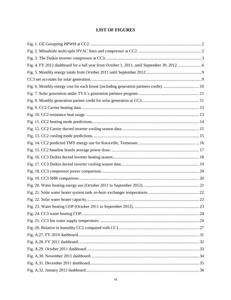
LIST OF FIGURES

Fig. 1. GE Geospring HPWH at CC2. .......................................................................................................... 2

Fig. 2. Mitsubishi multi-split HVAC lines and compressor at CC2. ............................................................ 2

Fig. 3. The Daikin inverter compressor at CC3. ........................................................................................... 3

Fig. 4. FY 2012 dashboard for a full year from October 1, 2011, until September 30, 2012. ...................... 6

Fig. 5. Monthly energy totals from October 2011 until September 2012. .................................................... 9

CC3 net accounts for solar generation. ......................................................................................................... 9

Fig. 6. Monthly energy cost for each house (including generation partners credit). .................................. 10

Fig. 7. Solar generation under TVA’s generation partners program. .......................................................... 11

Fig. 8. Monthly generation partner credit for solar generation at CC3. ...................................................... 11

Fig. 9. CC2 Carrier heating data. ................................................................................................................ 13

Fig. 10. CC2 resistance heat usage. ............................................................................................................ 13

Fig. 11. CC2 heating mode predictions. ...................................................................................................... 14

Fig. 12. CC2 Carrier ducted inverter cooling season data. ......................................................................... 15

Fig. 13. CC2 cooling mode predictions. ..................................................................................................... 15

Fig. 14. CC2 predicted TMY energy use for Knoxville, Tennessee. .......................................................... 16

Fig. 15. CC2 baseline hourly average power draw. .................................................................................... 17

Fig. 16. CC3 Daikin ducted inverter heating season. .................................................................................. 18

Fig. 17. CC3 Daikin ducted inverter cooling season data. .......................................................................... 19

Fig. 18. CC3 compressor power comparison. ............................................................................................. 20

Fig. 19. CC3 SHR comparison.................................................................................................................... 20

Fig. 20. Water heating energy use (October 2011 to September 2012). ..................................................... 21

Fig. 21. Solar water heater system tank–to-heat–exchanger temperatures. ................................................ 22

Fig. 22. Solar water heater capacity. ........................................................................................................... 22

Fig. 23. Water heating COP (October 2011 to September 2012). .............................................................. 23

Fig. 24. CC3 water heating COP................................................................................................................. 24

Fig. 25. CC3 hot water supply temperature. ............................................................................................... 24

Fig. 26. Relative in humidity CC2 compared with CC1. ............................................................................ 27

Fig. A.27. FY 2010 dashboard. ................................................................................................................... 31

Fig. A.28. FY 2011 dashboard. ................................................................................................................... 32

Fig. A.29. October 2011 dashboard. ........................................................................................................... 33

Fig. A.30. November 2011 dashboard. ....................................................................................................... 34

Fig. A.31. December 2011 dashboard......................................................................................................... 35

Fig. A.32. January 2012 dashboard............................................................................................................. 36

vii

Fig. A.33. February dashboard.................................................................................................................... 37

Fig. A.34. March dashboard. ...................................................................................................................... 38

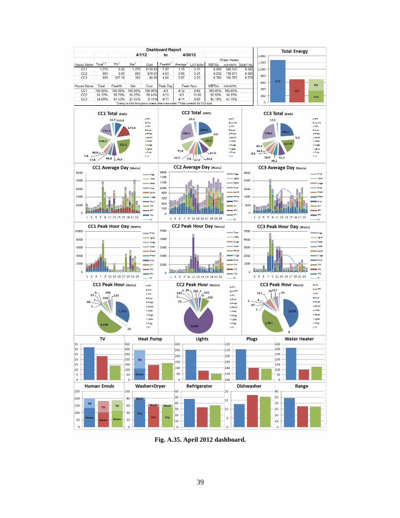
Fig. A.35. April 2012 dashboard................................................................................................................. 39

Fig. A.36. May 2012 dashboard. ................................................................................................................. 40

Fig. A.37. June 2012 dashboard. ................................................................................................................. 41

Fig. A.38. July 2012 dashboard. ................................................................................................................. 42

Fig. A.39. August 2012 dashboard. ............................................................................................................ 43

Fig. A.40. September 2012 dashboard. ....................................................................................................... 44

LIST OF TABLES

Table 1. FY 2012 annual kilowatt-hour usage by equipment for the three houses ....................................... 7

Table 2. Comparison of Appliance and WH System Energy Savings Potential in kWh. ............................. 8

Table 3. Heating degree days at 65 and departure from normal ................................................................ 10

ix

ABBREVIATIONS, ACRONYMS, and INITIALISMS

CC1 Builder House

CC2 Retrofit House

CC3 High-performance House

CDD cooling degree days

COP coefficient of performance

DHW domestic hot water

EF energy factor

EPRI Electric Power Research Institute

ERV energy recovery ventilators

GFX gravity-film heat exchanger

HDD heating degree days

HP heat pump

HPWH heat pump water heater

HVAC heating, ventilation, and air-conditioning

HSPF heating seasonal performance factor

kWh kilowatt-hour

LCUB Lenoir City Utilities Board

LED light-emitting diode

NOAA National Oceanic and Atmospheric Administration

OAT outdoor air temperature

ORNL Oak Ridge National Laboratory

PV photovoltaic

RH relative humidity

SEER seasonal energy efficiency ratio

SHR sensible heating ratio

TMY typical meteorological year

TVA Tennessee Valley Authority

1

1. INTRODUCTION AND PROJECT OVERVIEW

The Campbell Creek project is funded and managed by the Tennessee Valley Authority (TVA)

Technology Innovation, Energy Efficiency, Power Delivery and Utilization Office. Technical

support is provided under contract by the Oak Ridge National Laboratory (ORNL) and the

Electric Power Research Institute (EPRI). The project was designed to determine the relative

energy efficiency of typical new home construction, energy efficiency retrofitting of existing

homes, and high-performance new homes built from the ground up for energy efficiency.

This project will compare three houses that represented the current construction practices: a base

case (Builder House—CC1); a modified house that could represent a major energy-efficient

retrofit (Retrofit House—CC2); and a house constructed from the ground up to be a high-

performance home (High Performance House—CC3). To enable a valid comparison, it was

necessary to simulate occupancy in all three houses and heavily monitor the structural

components and the energy usage by component.

All three houses are two story, slab on grade, framed construction. CC1 and CC2 are

approximately 2,400 ft2. CC3 has a pantry option, primarily used as a mechanical equipment

room, that adds approximately 100 ft2. All three houses are all-electric (with the exception of a

gas log fireplace that is not used during the testing) and use air-source heat pumps for heating

and cooling. The three homes are located in Knoxville in the Campbell Creek Subdivision. CC1

and CC2 are next door to each other and CC3 is across the street and a couple of houses down.

The energy data collected will be used to determine the benefits of retrofit packages and high-

performance new home packages. There are over 300 channels of continuous energy

performance and thermal comfort data collection in the houses (100 for each house). The data

will also be used to evaluate the impact of energy-efficient upgrades on the envelope, mechanical

equipment, and demand-response options. Each retrofit will be evaluated incrementally, by both

short-term measurements and computer modeling, using a calibrated model.

This report is intended to document the comprehensive testing, data analysis, research, and

findings within the January 2011 through October 2012 timeframe at the Campbell Creek

research houses. The following sections will provide an in-depth assessment of the technology

progression in each of the three research houses. A detailed assessment and evaluation of the

energy performance of technologies tested will also be provided. Finally, lessons learned and

concluding remarks will be highlighted.

2

2. REVIEW OF THE TECHNOLOGY PROGRESSION

The following is a description of changes to equipment and technologies used in the three homes

from the initial design and construction.

Furniture was moved into the homes on March 31, 2009,

to provide a thermal mass more appropriate for testing

than an empty house.

A prototype GE heat pump water heater (HPWH) was

installed at CC2 on April 15, 2009, replacing the original

standard electric model (Fig. 1).

The dryer at CC1 was changed by GE on December 2009

to one of the same model used at the other two houses

(because of issues with the control board in the originally

installed dryer).

The prototype GE HPWH in CC2 was taken out of service

on March 22, 2010, and replaced with a commercially-

available version that had a more efficient compressor.

The change resulted in a unit with a higher field

coefficient of performance (COP) than the prototype.

A light-emitting diode (LED) lighting upgrade package was installed on September 30, 2010, at

CC3, an operation that involved replacing several of the compact fluorescent light fixtures in the

home with more efficient LED fixtures (The equipment and the cost of this package were

detailed in the May 2011 TVA Progress

Report).

A Moen thermostatic shower control

valve was installed in the master bath

of CC3 on November 16, 2011, to

reduce variation in the shower

temperatures (caused by inconsistent

delivery temperatures from the solar

thermal system). In addition, a new

Taco mixing valve was installed on the

solar thermal hot water system at CC3 a

week later, November 22, 2011, to

provide a more consistent hot water

delivery temperature to the home.

On December 21, 2010, a Mitsubishi

multi-split heating, ventilation, and air-

conditioning (HVAC) system with one 4-ton outdoor unit and eight indoor units began operation

at CC2 (Fig. 2). Refrigerant lines for the individual units were run through exterior walls and

Fig. 1. GE Geospring HPWH at CC2.

Fig. 2. Mitsubishi multi-split HVAC lines and compressor

at CC2.

3

along either the garage or the backside of the house to the branch boxes on the back wall of the

garage. The unit remained in service until January 2012, when it was shut down (a Carrier

Greenspeed system was installed - see related item later in this section). The Mitsubishi

equipment was removed from the home in May of

2012 and salvaged by TVA.

On November 19, 2010, a Daikin ducted inverter

HVAC system was installed at CC3 to replace the

baseline two-stage zoned system (Fig. 3). On

January 12, 2011, a 5 kW electric heat unit was

installed; and on January 28, 2012, that 5 kW unit

was replaced with a 3 kW heat unit.

Televisions were added to each house on March 8,

2011. At CC1, a 50 inch plasma TV was added that

had an average daily energy consumption of 1.04

kilowatt-hours (kWh) (with 8.5 hours per day of on

time). At CC2, a 55 inch liquid crystal diode (LCD)

TV was installed that had an average daily energy consumption of 0.77 kWh. At CC3, a 55 inch

LED/LCD TV was added with an average daily kWh consumption of 0.46 kWh.

A Mitsubishi Lossnay energy recovery ventilator (ERV) went into service at CC2 on March 25,

2011, to provide the required fresh air to that house. The Lossnay unit replaced the original Air

Cycler fresh air system initially installed at CC2.

Human emulators were installed in each house by the EPRI in 2011 and began running on May

12, 2011. There are two in each house: one in the kitchen provides sensible and latent load to

represent people spending time and cooking in the living space, and a second one in the master

bathroom represents the load from occupants in the bedroom space. The profile used is based on

the DOE Building America benchmark.

A heat recovery system was installed at CC3 in May 2011 to allow evaluation of a system

designed to capture waste heat from the shower, clothes washer, and dryer, and to use this waste

heat to offset some of the hot water energy needs of the house. The system included a gravity-

film heat exchanger (GFX) installed on a vertical section of drain line, a dryer exhaust heat

exchanger, a preheat tank for storing the captured heat, and a recirculation pump with associated

controls. After the 6-week test period concluded, the equipment remained in place; however, the

dryer heat exchanger and the recirculating pump use were discontinued and only the GFX

remains in use. Currently, only waste heat from the shower is still being captured.

On December 31, 2011, an attempt was made to drill for a potential geothermal system in CC2;

however, problems with geology forced the attempt to be aborted after only about a third of the

required depth was reached. The hole was grouted and capped according to code in

January 2012.

On January 16, 2012, a Carrier Greenspeed heat pump HVAC system with an inverter

compressor and variable-speed indoor blower went into service in CC2 to replace the Mitsubishi

Fig. 3. The Daikin inverter compressor at

CC3.

4

multi-split system. The Carrier system uses the existing zoned ductwork installed for the baseline

system.

A Sanden Integrated EcoCute CO2 HPWH was installed at CC2 on June 14, 2012, but it failed

because of damage incurred in shipping the unit from France. A replacement installed on August

10, 2012, was successfully tested. That unit was put into service heating the water for the house

on August 28, 2012.

5

3. OVERALL PERFORMANCE OF HOUSES FROM OCTOBER 1, 2011,

THROUGH SEPTEMBER 30, 2012

3.1 ANNUAL DASHBOARDS

Figure 4 shows the dashboard for a full year of performance from October 1, 2011, through

September 30, 2012. The annual energy consumption savings of CC2 and CC3 compared with

CC1 are 40% and 48%, respectively. The net energy savings of CC3 over CC1, accounting for

photovoltaics (PV) generation, is 66%. The peak hourly demand occurred on January 19, 2012,

at CC1 and CC2 and on September 5 at CC3. The peak demand in September was due to the

precooling study that occurred during that month. CC2 had a 50% lower absolute peak and CC3

a 51% lower peak. The load factors for the entire year are 0.17, 0.21, and 0.19 for CC1, CC2,

and CC3, respectively. The pie charts in Fig. 4 show the full-year energy demands for various

loads in each of the houses. Bar charts are provided to show the relative energy uses in all three

houses of the heat pumps, lights, plug loads, water heating, washer/dryer (combined),

refrigerator, dishwasher, human emulators, television, and range. The actual Lenoir City Utilities

Board (LCUB) residential rates and monthly hookup fee were used to calculate the costs.

Figure 4 also contains a pie chart showing the pieces that make up the total annual kilowatt-hours

used in the builder, retrofit, and high-performance house. In the builder house, the space heating

load makes up the largest fraction of energy usage, 21% of the total. The cooling load was 19%

and water heating energy another 19% of the total. The annual plug loads (including TV)

represent 15% and the lights also represent 15%. The dryer was 5% of the total builder house

load. In the retro house, heating is the largest piece at 32%, followed by plug loads 20%, cooling

13%, water heating 10%, lights 8%, and dryer 6%. In CC3, plug load were the largest piece at

22%, cooling 20%, heating 15%, water heating 15%, and the electric dryer 7%.

The FY 2012 annual energy consumption for the heat pump, water heater, lights, plug loads,

refrigerator, dishwasher, range, clothes washer, and dryer for all three houses is shown in

Table 1. The rightmost column shows the percentage of annual energy savings resulting from

each major energy user. The heat pump in CC2 used 33% less energy and the heat pump in CC3

used 55% less than the one in CC1 over the entire one year period. The energy savings for water

heating reflect not only the more efficient HPWH in CC2 and the solar water heater in CC3 but

also the measured 14 gallon reduction in hot water needed to wash clothes and dishes with the

ENERGY STAR® appliances in CC2 and CC3 that are not in CC1. The more efficient lighting in

CC2 and CC3 saved 69% and 79%, respectively, compared with the 100% incandescent lighting

installed by the builder in CC1. The energy for the ERVs that provide fresh air ventilation in

CC2 and in CC3 is included in the “HP” energy columns.

6

Fig. 4. FY 2012 dashboard for a full year from October 1, 2011, until September 30, 2012.

7

Table 1. FY 2012 annual kilowatt-hour usage by equipment for the three houses

Equipment/ appliances House Total % Savings

HP

CC1 7977

CC2 5384 33%

CC3 3601 55%

Water heater

CC1 3839

CC2 1241 68%

CC3 1528 60%

Lights

CC1 2930

CC2 916 69%

CC3 615 79%

Plug load

CC1 2504

CC2 2147 14%

CC3 2087 17%

Refrigerator

CC1 554

CC2 404 27%

CC3 445 20%

Dishwasher

CC1 162

CC2 211 30%

CC3 216 34%

Range

CC1 585

CC2 443 24%

CC3 444 24%

Washer

CC1 68

CC2 97 43%

CC3 98 45%

Dryer

CC1 1009

CC2 748 26%

CC3 751 26%

The refrigerators in CC2 and CC3 used 27% and 20% less energy than the refrigerator in CC1

over the one year period. The electric ranges in CC2 and CC3 used the smaller of the two ovens

available in the installed models, which led to a 26% percent energy savings compared with the

single larger oven in CC1 under the same simulated cooking load in all three houses.

The ENERGY STAR dishwasher in CC2 and CC3 actually used over 30% more energy than the

standard (non-ENERGY STAR) model in CC1. The ENERGY STAR model did save on hot

water consumption: CC2 used 113 fewer gallons and CC3 used 139 fewer gallons of hot water.

Based on 157 Wh/gal, the measured electrical energy required to heat water with the standard

electric water heater in CC1, the ENERGY STAR dishwashers realized an annual hot water

energy savings of only 15 and 18.5 kWh, respectively, for CC2 and CC3. Adjusting the numbers

8

in Table 1 to account for the energy used to heat the water supplied, the three dishwashers used

335, 367, and 368 kWh, respectively, in CC1, CC2, and CC3. Thus even with hot water savings,

the ENERGY STAR model used ~10% more energy annually than the non-ENERGY STAR

dishwasher model in CC1.

The ENERGY STAR front-load clothes washers in CC2 and CC3, which have a much higher-

speed spin cycle, used more energy than the conventional top-load clothes washer in CC1, as

shown in Table 1. However, the savings from reduced hot water demand and their capability to

force more water from the washed clothes resulted in dryer energy savings. The annual hot water

use by the CC1, CC2, and CC3 clothes washers was 4784, 1499, and 1558 gallons, respectively.

That is a savings of over 3200 gallons of hot water per year for the ENERGY STAR models. The

total kilowatt-hours required for washing clothes when energy to heat water is included is 819,

332, and 342 kWh respectively, a ~58% savings for the ENERGY STAR front-load machine

over the top-load machine. Considering both washer and dryer loads and the electrical energy to

heat water gives a combined savings of about 40% for laundry in CC2 and CC3 compared with

CC1.

Table 2 illustrates the savings potential for different appliance “suites” paired with different WH

systems and provides an interesting comparison of the energy use given any of the three WH

systems and any of the appliance “suites”. The months of August and September 2012 were

excluded from the CC2 efficiency averages due to installation of the Sanden water heater in that

house. Those values were replaced with linearly interpolated values from the July and

November data; and, since the performance of the HPWH didn’t vary too much from month to

month, this method provides a reasonable estimate. Estimated values are shaded in Table 2.

Table 2. Comparison of Appliance and WH System Energy Savings Potential in kWh.

HW Energy

Delivered

CC1

Standard Electric

CC2

HPWH

CC3

Solar Thermal

kWh (thermal) 157 Wh/gal 55 Wh/gal 84 Wh/gal

CC1

Standard Appliances 3261 3839 1358 2053

CC2

Energy Star Appliances 2862 3369 1192 1801

CC3

Energy Star Appliances +

GFX Shower Heat Recovery

2663 3135 1109 1676

Shaded areas denotes estimated values

Figure 5 shows the monthly whole house energy data. The annual whole house energy savings

for CC3 after accounting for onsite solar PV generation is 66%. The 2.5 kW peak solar PV

fraction is about 31% of the total kilowatt-hour demand of CC3.

A Carrier Greenspeed system was installed in CC2 on January 16 to replace the Mitsubishi

multi-split system. Since the Carrier system has a higher heating seasonal performance factor

(HSPF) and seasonal energy efficiency ratio (SEER) than the multi-split system, a reduction in

9

the total energy consumption of CC2 was expected. The impact of this retrofit can be seen in

Fig. 5. In January, CC2 energy use was 66% relative to CC1. However, in February CC2, energy

use dropped to only 54% relative to CC1. This drop in energy use is mainly attributed to the

installation of the Carrier Greenspeed.

Fig. 5. Monthly energy totals from October 2011 until September 2012.

CC3 net accounts for solar generation.

3.2 ENERGY USE

Heating degree days (HDD) and cooling degree days (CDD) were calculated for the entire year

using 60 minute data and a base of 65F. They are compared in Table 3 with the 30 year normal

data for the Knoxville area published by the National Oceanic and Atmospheric Administration

(Comparative Climatic Data–NOAA). Although the weather was cooler than normal in October

2011 and September 2012, the 12 month period of this report was the hottest October–September

period on record for the contiguous United States (NOAA, 2012). June and July, particularly,

were hotter than average, with July being the 10th warmest July recorded for Knoxville

(Knoxville New Sentinel, 2012). The period overall had 6.5% fewer HDDs at 65 and 11.7%

more CDDs than has been normal over the past 30 years.

10

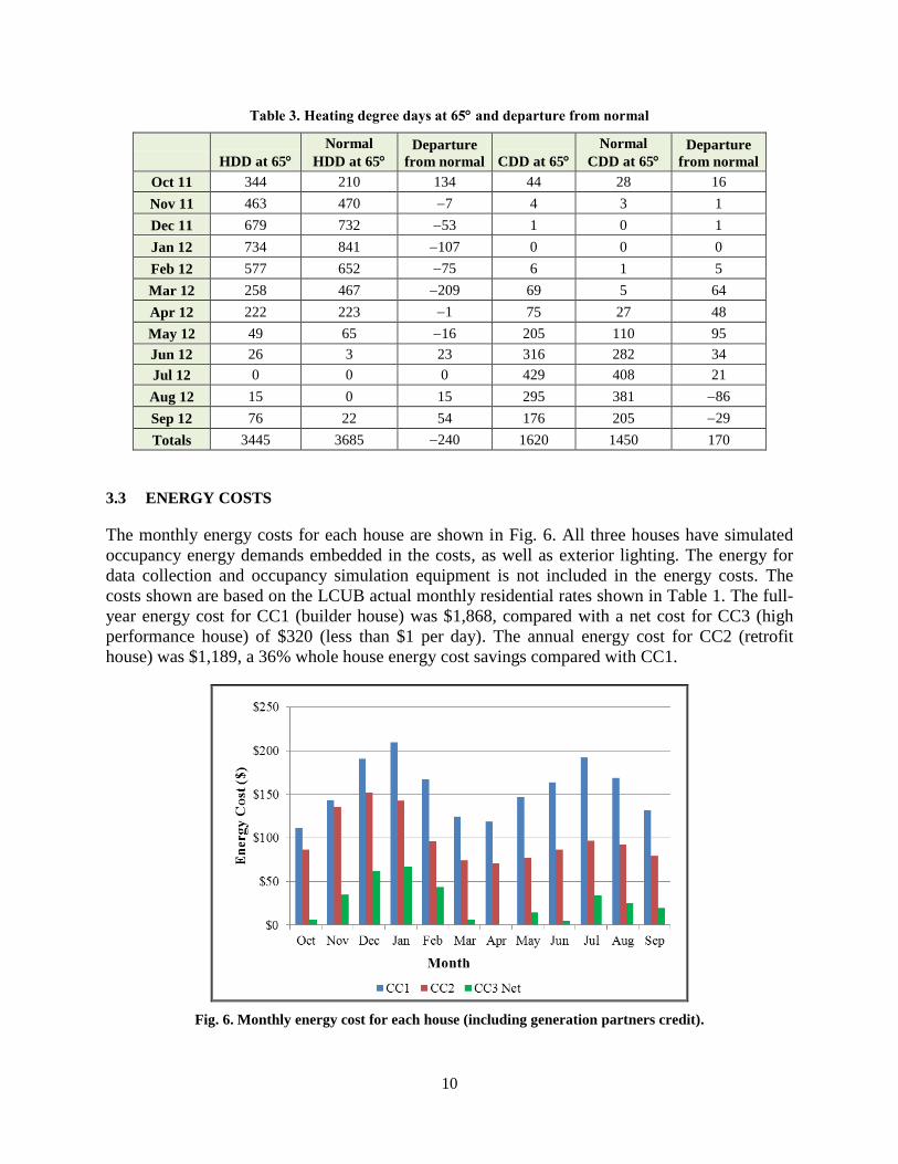
Table 3. Heating degree days at 65 and departure from normal

HDD at 65

Normal

HDD at 65

Departure

from normal CDD at 65

Normal

CDD at 65

Departure

from normal

Oct 11 344 210 134 44 28 16

Nov 11 463 470 7 4 3 1

Dec 11 679 732 53 1 0 1

Jan 12 734 841 107 0 0 0

Feb 12 577 652 75 6 1 5

Mar 12 258 467 209 69 5 64

Apr 12 222 223 1 75 27 48

May 12 49 65 16 205 110 95

Jun 12 26 3 23 316 282 34

Jul 12 0 0 0 429 408 21

Aug 12 15 0 15 295 381 86

Sep 12 76 22 54 176 205 29

Totals 3445 3685 240 1620 1450 170

3.3 ENERGY COSTS

The monthly energy costs for each house are shown in Fig. 6. All three houses have simulated

occupancy energy demands embedded in the costs, as well as exterior lighting. The energy for

data collection and occupancy simulation equipment is not included in the energy costs. The

costs shown are based on the LCUB actual monthly residential rates shown in Table 1. The full-

year energy cost for CC1 (builder house) was $1,868, compared with a net cost for CC3 (high

performance house) of $320 (less than $1 per day). The annual energy cost for CC2 (retrofit

house) was $1,189, a 36% whole house energy cost savings compared with CC1.

Fig. 6. Monthly energy cost for each house (including generation partners credit).

11

3.4 SOLAR AND GENERATION PARTNER CREDIT

The 2.5 kW peak solar system on CC3 generated 9.7 kWh/day average for the complete one year

test period. Generation averaged 11.4 kWh per day for the 6 month period of April through

September. The total annual energy cost savings for CC2 compared with CC1 is $1,549, an 83%

whole house energy cost savings compared with CC1. Savings from solar generation accounted

for $727, or 47% of the $1,549. The balance of the savings, $821 (53%), is due to energy

efficiency improvements. Figure 7 shows the monthly generation from the PV system, which

averaged 29 kWh/month. Figure 8 shows the monthly credit from solar energy production. The

monthly average for the complete year is $61, an average daily solar credit of $1.99.

Fig. 7. Solar generation under TVA’s generation partners program.

Fig. 8. Monthly generation partner credit for solar generation at CC3.

12

4. PERFORMANCE EVALUATION

4.1 HVAC COMPARISON—RETROFIT HOUSE CC2

In January 2012, a Carrier Greenspeed ducted inverter heat pump with zoning was installed in

CC2. The system is rated at 3-tons of cooling with an Air-Conditioning, Heating, and

Refrigeration Institute rated SEER of 20.5 and HSPF of 13.0. The fan coil was installed in the

sealed attic and connected to the existing ductwork. The system was split into two zones, with

one serving the upstairs and the other the downstairs.

Two prior systems have been installed at CC2, a single-stage, 16 SEER, 9.75 HSPF 3-ton heat

pump (which will be referred to as the baseline system) and a multi-split heat pump consisting of

a 15 SEER, 8.7 HSPF, 4-ton outdoor unit with an inverter-driven compressor and 8 high-wall

indoor units rated at either 0.75 ton (3 units) or 0.5 ton (5 units).

4.1.1 Heating Data

Previous reports (Munk, 2012) have detailed the performance of the Mitsubishi multi-split heat

pump. For this report, only the heating season performance of the Greenspeed system is

discussed; therefore, energy use prior to January 18, 2012, is not included in the following

analysis. The winter was fairly mild, but the system still did a very good job of minimizing the

need for resistance heat. In Fig. 9, the daily energy use is plotted against the average outdoor air

temperature (OAT). Because the Carrier system has a variable-speed compressor that can run at

higher speeds when the OAT is lower, it can significantly reduce the need for resistance heat as

supplemental heat. Most of the resistance heat use for the Carrier system was during defrost

cycles, when the resistance heat was used to prevent cold air from being blown into the house.

Figure 10 shows the resistance heat usage, in terms of energy and runtime, of the Carrier system

and the baseline system. Because of the mild winter, the data do not provide a complete picture

of the very-low-temperature resistance heat use of the Carrier system, but curve fits imply that

there would be roughly a 75–80% reduction compared with the baseline system. Figure 10 shows

the total energy use of the Carrier ducted inverter system compared with the baseline system; the

Carrier system shows significant energy savings. When these data are normalized by applying

them to typical meteorological year (TMY) data for Knoxville, Tennessee, the ducted inverter

system is predicted to save 1519 kWh (32%) compared with the baseline heat pump over a

typical heating season (Fig. 11). This is slightly more than the 25% savings than the HSPF

ratings would indicate.

13

0

10

20

30

40

50

60

70

10 15 20 25 30 35 40 45 50 55 60 65 70 75

Daily E

ner

gy U

se (kW

∙h)

Avg OAT ( F)Measured Predicted 95% Prediction Interval Resistance Heat

Fig. 9. CC2 Carrier heating data.

0

1

2

3

4

5

6

0

9

18

27

36

45

54

10 15 20 25 30 35 40 45 50 55 60 65 70

Da

ily

Ru

nti

me

(h)

Da

ily

En

erg

y U

se (

kW

-h)

Avg OAT ( F)

Carrier 20.5 SEER, 13.0 HSPF Amana 16.0 SEER, 9.5 HSPF

Poly. (Carrier 20.5 SEER, 13.0 HSPF) Poly. (Amana 16.0 SEER, 9.5 HSPF)

Fig. 10. CC2 resistance heat usage.

14

0

10

20

30

40

50

60

70

80

90

100

110

10 15 20 25 30 35 40 45 50 55 60 65 70 75

Daily E

ner

gy U

se (kW

∙h)

Avg OAT ( F)

Amana 9.75 HSPF Carrier 13.0 HSPF

Fig. 11. CC2 heating mode predictions.

4.1.2 Cooling Data

The cooling energy use through September 30, 2012, is plotted in Fig. 12. The cooling data show

very low energy use, with about a $2/day energy cost for cooling at $0.10/kWh during the hottest

days. Figure 13 shows the energy use compared with the two prior systems. The new ducted

inverter system also showed significant energy savings during the cooling season. Normalizing

the data to the TMY data for Knoxville predicts that the ducted inverter system will save 681

kWh (36%) compared with the baseline system. This is significantly more than the 22% savings

predicted by comparing the SEER ratings of the two units.

15

0

10

20

30

40

50

50 55 60 65 70 75 80 85 90

Daily E

ner

gy U

se (kW

∙h)

Avg OAT ( F)

Measured Predicted 95% Prediction Interval

Fig. 12. CC2 Carrier ducted inverter cooling season data.

0

5

10

15

20

25

30

35

40

45

50

55

60

50 55 60 65 70 75 80 85 90 95

Daily E

ner

gy U

se (kW

∙h)

Avg OAT ( F)

Amana 16.0 SEER Carrier 20.5 SEER

Fig. 13. CC2 cooling mode predictions.

16

4.1.3 Annual Performance

The TMY predictions for the heating and cooling season energy use are combined for an annual

energy use comparison in Fig. 14. Heating energy use was between 2.5 and 3 times more than

the cooling season energy use for all systems. The ducted inverter system shows an annual

savings of 2200 ±144 kWh, or 33%, over the baseline system.

1,9071,211

4,754

3,235

0

1000

2000

3000

4000

5000

6000

7000

Amana 16.0 SEER, 9.75

HSPF

Carrier 20.5 SEER, 13.0

HSPF

kW

-h

Heating Cooling

Fig. 14. CC2 predicted TMY energy use for Knoxville, Tennessee.

4.1.4 Hourly Peak Power

Of particular interest to utilities is reducing the peak power consumption of HVAC systems. The

ducted inverter system is capable of providing much higher heating capacities at lower

temperatures compared with traditional single- or two-speed heat pumps. This can allow the heat

pump to avoid the use of inefficient resistance heat and reduce the peak power draw. Figure 15 is

a plot of hourly power consumption regressions of the baseline system from 2010 and the ducted

inverter system for 2012. Because 2012 had such a mild winter, there is little very cold weather

data for the ducted inverter system; but at an OAT of 20°F, the system shows about a 25%

reduction in peak power draw while heating. The peak power reduction in cooling is more

significant, with the data showing an average 47% reduction at an OAT of 95°F.

17

0

1000

2000

3000

4000

5000

6000

7000

8000

0 10 20 30 40 50 60 70 80 90 100 110 120

Wa

tts

Average OAT ( F)

Amana

Carrier

Fig. 15. CC2 baseline hourly average power draw.

4.2 HVAC COMPARISON—HIGH-PERFORMANCE HOUSE CC3

The Daikin ducted inverter 18.0 SEER, 8.89 HSPF, 2-ton heat pump has been installed since

December 2010. The fan coil in CC3 is installed in a utility closet on the first floor instead of in

the attic as in CC2. There was no compatible zone control for the Daikin system, so it is set up as

a single zone with the thermostat located centrally on the first floor. The baseline system in this

house was an Amana two-stage, 15.0 SEER, 9.5 HSPF, 2-ton heat pump with zoning.

4.2.1 Heating Data

The heating energy use for the Daikin system from 2011 and 2012 is plotted in Fig. 16. The new

data match very well with the older data and indicate that the unit performance has not changed

significantly. Late in February, representatives from Daikin visited to investigate concerns that

the unit was not modulating as expected. This concern was documented in a prior report (Munk

2012), in which the unit was shown to run at near constant power throughout each cycle. During

the visit, the refrigerant charge was checked and an additional 14 ounces was added to the

system. No other issues were discovered during the visit. Given the limited heating data

following the visit, there was not sufficient data to determine if the charge adjustment had any

impact on the heating performance. Unlike the Carrier system at CC2, the Daikin system does

not use resistance heat during defrost cycles. Therefore, the Daikin system did not use any

resistance heat between October 2011 and September 2012.

18

0

5

10

15

20

25

30

35

40

45

50

10 15 20 25 30 35 40 45 50 55 60 65 70 75

Daily E

ner

gy U

se (kW

∙h)

Avg OAT ( F)

Measured Heating Data 1/9/2011 to 1/6/2012 Prediction (2011 Data)

95% Prediction Interval New Measured Data 1/7/2012 to 4/1/2012

Fig. 16. CC3 Daikin ducted inverter heating season.

4.2.2 Cooling Season

Since the Daikin system does not have zoning capability, the existing zoning dampers and room

registers are adjusted seasonally to maintain similar temperatures on the first and second levels.

During the summer, the downstairs requires significantly less cooling than the upstairs; so to

achieve a reasonable temperature balance, the downstairs damper was closed completely.

Although the arrangement provided consistent temperatures, it had the unintended effect of

reducing the system airflow. The fan coil does have a variable-speed brushless permanent

magnet motor; however, closing the downstairs damper increased the external static pressure

enough that the motor was no longer able to maintain the desired airflow. When the issue was

discovered, the reduced airflow was measured and the damper was opened enough to allow the

motor to reach the target airflow. For analysis, the data were separated into two sets, one with the

downstairs damper partially open and the other with the downstairs damper closed, as seen in

Fig. 17. These two data sets from the 2012 cooling season were compared with the data from the

2011 heating season. The 2012 data indicate slightly worse performance at lower average OATs

and slightly better performance at higher OATs. The data do all fall within the 95% confidence

prediction intervals that were generated from the 2011 data.

19

0

5

10

15

20

25

30

35

50 55 60 65 70 75 80 85 90 95

Daily E

ner

gy U

se (kW

∙h)

Avg OAT ( F)2011 Data Predicted (2011) 95% Prediction Interval (2011)

2012 Data (Damper Open) Predicted (2012 Damper Open) 2012 Data (Damper Closed)

Predicted (2012 Damper Open)

Fig. 17. CC3 Daikin ducted inverter cooling season data.

The damper-open and damper-closed data sets were analyzed and predictions were generated for

the entire 2012 cooling season for both sets. These were compared in order to determine if the

difference in the data sets was statistically significant and, if so, the magnitude of the difference.

The predicted energy difference indicated that with the downstairs damper closed, the system

would have used 137 ± 40 kWh more energy (with 95% confidence) than if the damper was only

partially open and the blower could reach the target airflow. This translates into a 7.6% ± 2.2%

increase in energy use. This is only a modest penalty for what was a significant, ~38%, reduction

in airflow. Figures 18 and 19 show a comparison between the compressor power and sensible

heat ratio (SHR) plotted versus OAT for periods when the downstairs damper was partially open

and periods when it was fully closed. The plots show a significant decrease in compressor power

when the damper was closed, but the SHR was virtually the same. For the SHR to be the same,

the total cooling capacity had to have been reduced by approximately the same percentage that

the airflow was reduced. The drop in compressor power indicates that the reduced capacity was

likely a result of the variable-speed compressor running at lower speeds. It is likely that the

system reduced the compressor operating speed in response to the reduced airflow caused by the

downstairs damper being closed. The net result was reduced capacity and only slightly reduced

performance.

20

Fig. 18. CC3 compressor power comparison.

Fig. 19. CC3 SHR comparison.

4.3 WATER HEATER COMPARISON

Three types of water heating systems have been installed at the Campbell Creek homes. CC1 has

a 0.9 energy factor (EF), 40 gallon electric water heater installed in the garage. CC2 had an R-

134a HPWH with a 2.35 EF rating installed until August 2012. In September 2012, a CO2

HPWH was installed, and it operated for the remaining timeframe studied in this report. Both

units were installed in the garage. CC3 has a solar thermal water heating system. This system

uses a secondary fluid to pick up heat from the solar absorbers and a brazed plate heat exchanger

to transfer the heat to the domestic hot water. An 80 gallon storage tank with backup resistance

heat installed in a utility room is used to store the heated water, and a mixing valve is used to

temper the water down to a target temperature of 120°F.

The past 12 months of energy use for water heating at all three homes is plotted in Fig. 20. As

expected, the standard electric water heating in CC1 used the most energy for all months and had

higher use in the winter months when the incoming water temperature was lower. The water

heating energy use for CC2 is more consistent throughout the year and is a quarter to a third of

the energy use at CC1. The energy use of the solar system at CC3 follows a similar trend but

deviates from past energy use data. The next section presents an in-depth look at these

deviations.

21

0

50

100

150

200

250

300

350

400

450

En

erg

y U

se (

kW

-h)

CC1 CC2 CC3

Fig. 20. Water heating energy use (October 2011 to September 2012).

Since the solar system draws water from the bottom of the tank for water heating, adjusting the

lower element thermostat also increased the temperature of the water entering the solar system’s

heat exchanger (Fig. 21). This reduced the opportunities for solar heating and reduced the

efficiency of the heat transfer. Although the tank temperature sensor was moved to a better

position, the more frequent use of the bottom element also led to more cycles in which the solar

system was not actually capable of heating the water, as can be seen in Fig. 22.

The water heating COP has been calculated for the system by dividing the amount of heat

delivered from the storage tank by the total energy use of the system Fig. 23. Therefore, this

number includes the effect of heat loss from the storage tank. The COP of the standard electric

water heater in CC1 is very consistent and varied only between 0.84 and 0.86. This indicates that

the seasonal difference in tank losses have minimal impact on the system efficiency, despite the

fact that the average garage temperature varied by more than 20°F between winter and summer

months. The R-134a HPWH installed in CC2 showed very good performance throughout the

year with COPs ranging from 2.2 to 2.6. The installation of the CO2 HPWH was taking place in

August, and there were some operational issues at startup that caused the low COP. September

was a whole month of good data for the CO2 HPWH though, and it showed very promising

performance with a COP of 2.7.

22

Fig. 21. Solar water heater system tank–to-heat–exchanger temperatures.

-6000

-4000

-2000

0

2000

4000

6000

8000

10000

1/1/11 1/31/11 3/2/11 4/2/11 5/2/11 6/2/11 7/2/11 8/1/11 9/1/11 10/1/11 11/1/11 12/1/11

Ca

pa

cit

y (

Btu

/h)

Lower element thermostat adjusted to heat tank up to 120°F

Fig. 22. Solar water heater capacity.

23

0

1

2

3

4

5

6

CO

P (

W/W

)

CC1 CC2 CC3

Fig. 23. Water heating COP (October 2011 to September 2012).

The solar thermal system in CC3 shows a wide range of COPs throughout the year. To fully

explain the operational performance of the system, the COP of the unit was plotted from data

over the last three years in Fig. 24. As seen in the plot, the performance was significantly higher

in 2010 than in most of the corresponding months in later years. It was observed in June 2011

that the resistance heating element in the storage tank was not heating the water up to the 120°F

setpoint. This was being masked by the fact that the tempering valve was set too high, causing

the system to supply water hotter than 120°F to the house soon after the solar system had run and

water cooler than 120°F when the solar system had not been running. This phenomenon can be

seen in Fig. 25, which plots the hot water temperature to the house during water draws for the

year of 2011. In June 2011 the water heater thermostats were adjusted to heat the tank to the

desired 120°F set point, and the tempering valve was adjusted downward to limit the hot water

supply temperature to 120°F. The result was a much tighter band of hot water supply

temperatures.

In June 2011, the temperature sensor for the solar system was securely attached to the lower

element nut. Previously, it was sitting loosely in the lower element/thermostat compartment. The

solar system compares the temperature at the solar collector with the tank temperature; when a

12°F temperature difference is sensed, the solar system turns on. With the tank temperature

sensor more securely attached to the lower element nut, it probably read a higher temperature

than before; therefore, a comparatively higher temperature at the solar collector would be

required to turn the solar system on.

24

Fig. 24. CC3 water heating COP.

Fig. 25. CC3 hot water supply temperature.

25

In February 2012 it was observed that the solar system was shutting off even while the domestic

hot water was still picking up significant heat from the heat exchanger. The temperature

differential was adjusted downward to force the solar thermal system to run longer before

shutting off. The net effect of this change is not fully apparent in the data, however, because the

May 2012 data seem to be on the low end, whereas the June 2012 data are quite good when

compared with the 2011 data. In June 2011 the flow rate on the source side was adjusted to

match the sink side in the heat exchanger in an attempt to increase the efficiency. June had a

period when the power to the resistance heat was removed, which allowed the lower tank

temperature to drop below the typical level. This allowed the solar thermal system to run more

and at higher efficiencies. The July to September 2012 data indicate that the adjustment did not

have a significant impact on the water heating energy use.

The lower element thermostat setting from 2010 to June 2011 was not high enough to guarantee

that the water leaving the tank was kept near 120°F; however, this typically was not an issue

because of the higher degree of stratification seen in the tank as a result of the solar system. A

typical electric water heater may see only a 15°F difference between the upper tank temperature

and lower tank temperature before the lower element turns on. Since the solar system can heat

the water in the tank to temperatures well above the 120°F setpoint, the tank may still have

plenty of hot water in the upper half when the lower half drops below the thermostat close

temperature.

There is great potential for savings by optimizing the resistance heat use of a solar thermal

system, as shown by the performance difference between the system in 2010 compared with that

in the latter half of 2011 and 2012. With the current control mechanism for the resistance heating

element, a compromise must be made between ensuring the availability of hot water and

increased efficiency.

26

5. LESSONS LEARNED AND CONCLUSIONS

CC1 consumed 19,883 kWh of total energy during FY 2012; CC2 used approximately 40% less

and CC3 approximately 48% less. However, since PV supplied 3,535 kWh of the total load, CC3

required 66% less energy from the grid for FY 2012. In addition to the valuable insight provided

by the reduction in energy consumption afforded by the various combinations of energy

conservation measures in the three homes, other key points of interests and lessons gleaned from

over the past year are described below.

HVAC: It is very difficult to maintain consistent temperature levels between the first and second

levels of a home without some sort of zoning. If zoning is employed, then the ducts should be

sized with this in mind. Zoning will likely require that the ducts be larger in order to handle

additional airflow when the other damper(s) are closed while avoiding performance penalties due

to reduced airflow or increased blower power.

A system with a variable-speed compressor is more likely to mask inherent system problems

unless it has a sufficiently sophisticated control system to communicate issues with the

homeowner. In trying to balance the temperatures of the first and second floors, we had to close

the downstairs damper completely. Doing so increased the external static pressure of the duct

system enough to reduce indoor cooling airflow by 37%, which in a typical system would

probably lead to a frozen evaporator coil. However, the variable-speed compressor was able to

compensate for the reduced airflow with only a minor penalty in performance. It is good that the

system can stay running with only a minor efficiency penalty; however, its ability to do so could

lead to problems going undiagnosed and result in systems running at less than peak efficiencies.

Water Heater: The method of controlling the backup heat in a solar thermal system can have

large impacts on energy consumption. There is a balance between guaranteeing enough hot water

and unnecessarily using resistance heat. The solar system is attached to an 80 gallon storage

tank, whereas the other houses have only 40–50 gallon tanks. In the future, we may be able to

disable the lower element thermostat on the solar system and set the upper element to come on at

around 120°F and still ensure that there is hot water available without using the resistance heat

excessively. This will allow the water in the bottom of the tank to get much colder, which will

provide more favorable temperatures for the solar water heating system.

The HPWH has provided very consistent COPs, between 2.2 and 2.6, compared with the solar

water heating system. This is particularly true in light of the variability possible as a result of the

different backup heating control methods in solar water heating systems. The solar system

definitely has the potential to provide higher efficiencies, but it will probably require some

tweaking and experimentation to reach optimal performance. The performance of the solar

system will also be more dependent on the hot water use patterns of the occupants. Water draws

late in the evening and early in the morning often deplete the hot water generated during the day

and require the use of backup heat. If occupants could tailor their hot water use to better coincide

with the availability of solar heating, then performance would be improved further.

High Relative Humidity (RH) at CC2: Higher indoor RH at CC2 compared with CC1 was

observed during the summers of 2010, 2011, and 2012 (Fig. 26). A different HVAC unit was

used in CC2 during each summer. Although some of the RH difference between the summers

27

Fig. 26. Relative in humidity CC2 compared with CC1.

might be due to the difference in HVAC units at CC2, that does not explain the consistent higher

level of summer RH at CC2 than at CC1.

Based on analysis of temperature/RH sensors on the roof deck, in the attic air, on the attic floor,

and in the second level of the retrofit home, it is possible that the source of moisture in the

conditioned space might be the attic. Experiments are ongoing, focused on the roof as a possible

moisture infiltration point, to understand the high RH levels in CC2.

Precooling for Peak Energy Shaving: ORNL investigated the impact of precooling a home and

letting it coast through the on-peak time (12–8 p.m.) using a calibrated model of CC1. Model

analysis showed that precooling used 13% more cooling energy than a flat 78°F schedule for the

whole summer. However, on sunny days with high outdoor temperatures, the on-peak (12–8

p.m.) energy savings resulting from a precooling schedule compared with a flat 78°F schedule

were as high as 60%. The precooling schedule that was modeled was programmed in the

thermostats at all the Campbell Creek homes on September 4 and continued until September 25;

it can be used for further analysis of precooling strategies.

28

6. PUBLICATIONS

Biswas, Kaushik, Anthony Gehl, Roderick Jackson, Philip Boudreaux, and Jeffrey Christian.

2012. Comparison of Two High-Performance Energy Efficient Homes: Annual Performance

Report, December 1, 2010–November 30, 2011, ORNL/TM-2011/539. Oak Ridge, TN: Oak

Ridge National Laboratory.

Boudreaux, Philip, Anthony Gehl, and Jeffrey Christian. 2012. Occupancy Simulation in Three

Residential Research Houses, ASHRAE Transactions, vol. 118. Pt. 2.

Boudreaux, Philip, Timothy Hendrick, Jeffrey Christian, and Roderick Jackson. 2012. Deep

Residential Retrofits in East Tennessee, ORNL/TM-2012/109. Oak Ridge, TN: Oak Ridge

National Laboratory.

Munk, Jeffrey D., Anthony C.Gehl, and Roderick K. Jackson. 2012. Performance of Variable

Capacity Heat Pumps in Mixed Humid Climates, ORNL/TM-2012/17. Oak Ridge, TN: Oak

Ridge National Laboratory.

Tomlinson, John, Jeffrey Christian, and Anthony Gehl. 2012. Evaluation of Waste Heat

Recovery and Utilization from Residential Appliances and Fixtures, ORNL/TM-2012/243, Oak

Ridge, TN: Oak Ridge National Laboratory.

Christian, Jeffrey, Anthony Gehl, Philip Boudreaux, Joshua New, and Rex Dockery. 2010.

Tennessee Valley Authority’s Campbell Creek Energy Efficient Homes Project: 2010 First Year

Performance Report July 1, 2009–August 31, 2010, ORNL/TM-2010/206. Oak Ridge, TN: Oak

Ridge National Laboratory.

29

7. REFERENCES

Knoxville News Sentinel. 2012, “Ouch! July in US was hottest ever in history books,” (August 8,

2012), retrieved November 11, 2012, from Knoxnews.com,

http://www.knoxnews.com/news/2012/aug/08/ouch-july-in-us-was-hottest-ever-in-

history/?print=1.

“Comparative Climatic Data (n.d.),” retrieved November 1, 2012, from National Climatic Data

Center, “Normal Monthly Heating Degree Days (Base 65),”

http://www.ncdc.noaa.gov/oa/climate/online/ccd/nrmhdd.html

Munk, J. D. 2012. Performance of Variable Capacity Heat Pumps in Mixed Humid Climates.

Oak Ridge National Laboratory, April.

NOAA (National Oceanographic and Atmospheric Administration. 2012, NOAA National

Climatic Data Center, State of the Climate: National Overview for September 2012, published

online October 2012, retrieved on November 2, 2012,

http://www.ncdc.noaa.gov/sotc/national/2012/9.

31

APPENDIX A

PAST ANNUAL DASHBOARDS

Fig. A.27. FY 2010 dashboard.

32

Fig. A.28. FY 2011 dashboard.

33

MONTHLY DASHBOARDS

Fig. A.29. October 2011 dashboard.

34

Fig. A.30. November 2011 dashboard.

35

Fig. A.31. December 2011 dashboard.

36

Fig. A.32. January 2012 dashboard.

37

Fig. A.33. February dashboard.

38

Fig. A.34. March dashboard.

39

Fig. A.35. April 2012 dashboard.

40

Fig. A.36. May 2012 dashboard.

41

Fig. A.37. June 2012 dashboard.

42

Fig. A.38. July 2012 dashboard.

43

Fig. A.39. August 2012 dashboard.

44

Fig. A.40. September 2012 dashboard.

45

FACT SHEET

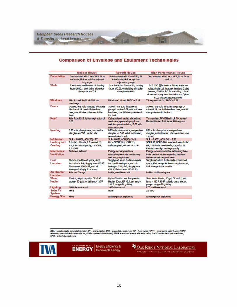
46