camera calibration and light source orientation from solar...

www.elsevier.com/locate/cviu

Computer Vision and Image Understanding 105 (2007) 60–72

Camera calibration and light source orientation from solar shadows

Xiaochun Cao *, Hassan Foroosh

Computational Imaging Laboratory, University of Central Florida, Orlando, FL 32816-2362, USA

Received 2 March 2006; accepted 10 August 2006Available online 26 September 2006

Abstract

In this paper, we describe a method for recovering camera parameters from perspective views of daylight shadows in a scene, givenonly minimal geometric information determined from the images. This minimal information consists of two 3D stationary points andtheir cast shadows on the ground plane. We show that this information captured in two views is sufficient to determine the focal length,the aspect ratio, and the principal point of a pinhole camera with fixed intrinsic parameters. In addition, we are also able to compute theorientation of the light source. Our method is based on exploiting novel inter-image constraints on the image of the absolute conic andthe physical properties of solar shadows. Compared to the traditional methods that require images of some precisely machined calibra-tion patterns, our method uses cast shadows by the sun, which are common in natural environments, and requires no measurements ofany distance or angle in the 3D world. To demonstrate the accuracy of the proposed algorithm and its utility, we present the results onboth synthetic and real images, and apply the method to an image-based rendering problem.� 2006 Elsevier Inc. All rights reserved.

Keywords: Camera calibration; Solar shadow; Light source orientation estimation; Planar homology

1. Introduction

Camera calibration is an essential step in computervision for 3D Euclidean reconstruction and motion estima-tion. It also plays a crucial role in applications such as aug-mented reality, and production of special effects.Techniques from augmented reality and inverse renderingnow permit the rendering of synthetic models within imag-es or video sequences. However, in order for these tech-niques to be successful, cameras need to be calibrated toensure that real and computer generated objects blend ina geometrically correct fashion in their mixed environment.On the other hand, to create realistic and seamless images,virtual objects have to be shaded consistently under the realillumination condition of the target scene, which in partic-ular requires the knowledge of the light source direction.There is, therefore, an increasing need for calibration and

1077-3142/$ - see front matter � 2006 Elsevier Inc. All rights reserved.

doi:10.1016/j.cviu.2006.08.003

* Corresponding author.E-mail addresses: [email protected] (X. Cao), [email protected]

(H. Foroosh).

light source estimation directly by using minimal informa-tion from the images of the target scene.

Traditional camera calibration methods use a calibra-tion object with a fixed 3D geometry [10,15,44]. Recently,more flexible plane-based approaches [11,12,23,26,40,50]have been proposed that use the orthonormal propertiesof the rotation matrix, which represents the relative rota-tion between the 3D world and the camera coordinate sys-tem. Zhang [50] has shown that it is possible to calibrate acamera using a planar pattern viewed at a few different ori-entations. Sturm and Maybank [40] extended this tech-nique, and obtained the solution for the case when thecamera intrinsic parameters can vary. Gurdjos et al. [11]formulated the plane-based calibration problem in a moreintuitive geometric framework according to Poncelet’s the-orem, which makes it possible to give a Euclidean interpre-tation to the plane-based calibration techniques. Otherspecial objects (see Fig. 1), e.g. balls or spheres [1,41,49],surfaces of revolution [8,46], circles [7,18,28,47], non-tex-tured Lambertian surfaces [19], fixed stars in the nightsky [20] and 1D objects [51], have also been used in the past

mailto:[email protected]

mailto:[email protected]

Fig. 1. A summary list of previous camera calibration objects. (a) 3D square grid [44]. (b) 3D circular grid [15]. (c) 2D square grid [40,50]. (d) Architecturalbuildings [23]. (e) Balls or spheres [1,41,49]. (f) Coplanar circles [7,18,28,47]. (g) Surfaces of revolution [8,46]. (h) Fixed stars in the night sky [20]. Note thatthis figure is by no means complete and only representative work is listed.

X. Cao, H. Foroosh / Computer Vision and Image Understanding 105 (2007) 60–72 61

as alternative calibration objects. Although the recentauto-calibration techniques [14,27,33,38] avoid the oneroustask of using special calibration objects, they mostlyrequire more than three views and also assume a simplifiedcamera model.

The calibration technique introduced in this paper,namely, calibration from shadows, is closely related tothe existing methods [6,8,21,23,25,40,46,50] that explorethe constraints provided by vanishing points along orthog-onal directions, or the pole–polar relationship in terms ofthe geometry of the image of the absolute conic (IAC).However, it relaxes some of the constraints found in previ-ous calibration algorithms such as [23], which requires fourviews to obtain four intrinsic parameters from a pair of 3Dstationary points and their cast shadows. Our method isbased on exploiting some novel inter-image constraintson the camera intrinsic parameters. We show that two cor-responding image projections of the same 3D line on theground plane provide two additional constraints on thecamera intrinsic parameters. Consequently, two views areenough to determine the aspect ratio, the focal length,and the principal point.

Shadows are important in our perception of the world[32], because they provide important visual cues for depthand shape. They are also useful for computer vision appli-cations such as building detection [24], surveillance systems[16,17,29,30,34,39] and inverse lighting [31,37]. However,shadows are not frequently exploited in 3D vision. Somefew examples include the work on the relationship betweenthe shadows and object structure by Kriegman and Bel-humeur [22], the work on object recognition by Van Goolet al. [45], and the work on weak structured lighting byBouguet and Perona [3]. Shadows are interesting for cam-era calibration since the shadows of two parallel lines caston a planar surface by an infinite point light source (e.g. thesun), are also parallel, which together with the vertical van-ishing point provide orthogonal constraints on the imageof the absolute conic.

This paper extends the work in [4] by providing a solu-tion to a more general and flexible geometric configura-tion, where the requirement for vertical objects iseliminated, with full performance evaluation and the anal-ysis of degenerate cases. Our geometric constructions are

close to the ones in [36] and [2]. However, our work is dif-ferent from Reid and North’s work [36] in three respects:First, we estimate the camera parameters and the lightsource orientation, while they focus on the problem ofaffine reconstruction of a ball out of the ground plane.Second, their main input is the image of the groundplane’s horizon line, whereas in our case we assumeinstead the knowledge of the vertical vanishing point.Third, our major contribution is the inter-image con-straints on the IAC, which lead to the use of only twoimages. Although Antone and Bosse [2] used shadowsfor camera calibration and a setup similar to ours, theyrequire world-to-camera correspondences. Different fromtheir techniques, the contribution of our method lies onrelaxing the requirement of knowing 3D quantities, andon calibrating the camera from the informationdetermined only from the images.

The remainder of this paper begins with an introductionto the theoretical background in Section 2. We thendescribe our calibration method in Section 3, followed byimplementation details in Section 4, and the discussion ofthe degenerate configurations in Section 5. Finally, in Sec-tion 6 we present our results for both synthetic data andreal images, and demonstrate applications to image-basedrendering.

2. Theoretical background

2.1. Pinhole camera model and the image of the absolute

conic

A 3D point M = [X Y Z 1]T and its corresponding imageprojection m = [u v 1]T are related via a 3 · 4 matrix P by

m � K½r1r2r3t�|fflfflfflfflffl{zfflfflfflfflffl}PM;K ¼f c u0

0 kf v0

0 0 1

264

375; ð1Þ

where � indicates equality up to multiplication by a non-zero scale factor, ri are the columns of the rotation matrixR, t is the translation vector, and K is a non-singular 3 · 3upper triangular matrix known as the camera calibrationmatrix including five parameters, i.e. the focal length f,

v

zv

2t

1sπ

2s

1t1π

sv

1v

∞l

a

Fig. 2. Basic geometry of a scene with two stationary points t1 and t2

casting shadows s1 and s2 on the ground plane p by the distant light sourcev, i.e. the sun. p1 is the plane perpendicular to the ground plane that ispassing through the two points t1 and t2. l1 is the horizon line of theground plane p, where the any parallel lines in the ground plane throughthe two shadow points would meet, e.g. the point vs.

62 X. Cao, H. Foroosh / Computer Vision and Image Understanding 105 (2007) 60–72

the skew c, the aspect ratio k and the principal point at(u0,v0).

The IAC, denoted by x, is an imaginary point conicdirectly related to the camera internal matrix K in Eq. (1)via x = K�T K�1, which can be expanded up to a non-zeroscale as

x �

1 � cf k

cv0�kfu0

f k

� f 2þc2

f 2k2 � c2v0�ckfu0þv0f 2

f 2k2

� � v20ðf 2þc2Þ�2cv0kfu0

f 2k2 þ f 2 þ u20

26664

37775; ð2Þ

where the lower triangular elements are replaced by ‘‘*’’ tosave space, since x is symmetric. Instead of directly deter-mining K, it is possible to compute the symmetric matrix x

or its inverse (the dual image of the absolute conic), andthen compute the calibration matrix uniquely using eitherCholesky decomposition [35] or the following set ofequations as described in [4,50]:

k ¼ffiffiffiffiffiffiffiffiffiffiffiffiffiffiffiffiffiffiffiffiffiffiffiffiffiffiffiffi1=ðx22 � x2

12Þq

;

v0 ¼ðx12x13 � x23Þ=ðx22 � x212Þ;

u0 ¼� ðv0x12 þ x13Þ;

f ¼ffiffiffiffiffiffiffiffiffiffiffiffiffiffiffiffiffiffiffiffiffiffiffiffiffiffiffiffiffiffiffiffiffiffiffiffiffiffiffiffiffiffiffiffiffiffiffiffiffiffiffiffiffiffiffiffiffiffiffiffix33 � x2

13 � v0ðx12x13 � x23Þq

;

c ¼� f kx12; ð3Þ

where xij denotes the element in ith row and jth column ofx.

2.2. Calibration from vanishing points

In [23], Liebowitz and Zisserman formulated the calibra-tion constraints provided by vanishing points of mutuallyorthogonal directions in terms of the geometry of x. Theorthogonality relations provide linear constraints in termsof the elements of x, which can be readily used to calibratea camera [8,23,40,46,50]. The earlier result reported byCaprile and Torre in [6] is a special case where the camerahas zero skew and unit aspect ratio. Zhang’s flexible cali-bration method [50] uses the orthogonal property of thecolumns r1 and r2 of the rotation matrix R in Eq. (1), i.e.pT

1 xp2 ¼ 0, where pi (hi in [50], i = 1,2) denotes the ith col-umn of the projection matrix P. This is actually equivalentto the constraint vT

x xvy ¼ 0, where vx and vy are the vanish-ing points along the world X- and Y-axis, respectively,because p1 is the scaled vanishing point vx of the ray alongthe direction [100]T, and similarly p2 is the scaled vanishingpoint vy of the ray along the direction [010]T. It is impor-tant to mention that the above derivation does not apply tothe normal property of r1 and r2, i.e. pT

1 xp1 � pT2 xp2 ¼ 0

used in [40,50], since in general vx and vy have differentscales, which the authors in [40,50] determine by assumingknown world-to-image homographies. In [8,46], the pole–polar relationship with respect to x is exploited, whichstates that the vanishing line l of a plane is related to thevanishing point v of the normal direction to the plane via

l = xv. This is because any vanishing point x that isorthogonal to v must satisfy xTxv = 0. The importantpoint now is that this is true for any point x satisfying xT

l = 0, from which it follows that l = xv.These intra-image orthogonal constraints, together with

the novel inter-image constraints that we refer to as the‘‘weak pole–polar’’ relationship introduced in this paper,will be used later in Section 3 to derive a simple techniquefor camera calibration from shadows. The weak pole–polar

relationship here means that the two independent constraints

on x arising from the pole–polar relationship can not be

identified from a single view.

3. The method

In this section, we first examine the geometry of thescene and then introduce novel inter-image constraintsassociated with the weak pole–polar relationship for cameracalibration. Finally, we show how to compute the orienta-tion of the light source.

3.1. Scene geometry

The basic geometry of a scene containing two stationarypoints and their shadows on the ground plane cast by aninfinite point light source is shown in Fig. 2. Note that thisfigure shows the image projections of the 3D world pointsdenoted by corresponding lower-case characters. Forexample, the world point T1 (not shown in Fig. 2) ismapped to t1 in the image plane.

It is important to point out here that our configurationshown in Fig. 2 is different from [2,4,36], which requiredtwo vertical objects and their shadows. Although, similarto [2,4,36], we assume known vertical vanishing point vz

and known ground plane inter-image homography Hp,our configuration does not assume the use of verticalobjects. In other words as shown in Fig. 2 any pair ofobject points in 3D space and their shadows would be suf-

2b

1s π

2s

1bsv

∞l

xv

1v

2v

Fig. 3. The inter-image constraints in Eq. (12) can be applied to anycorresponding ground lines between two views (except for bisi). Forexample, we have the image correspondences, b1b2 and b 01b 02, of the 3Dline B1B2 between two views, and thus have the inter-image constraints onthe vanishing point vx, which is the intersection of the line b1b2 and l1.


ficient to perform calibration from two views. Let us nowdenote the orthogonal projections of the 3D points t1 andt2 in the ground plane as b1 and b2, which we shall hereafterrefer to as the footprints of the 3D points. In [2,4,36], theassumption is that the footprints are available and hencethe vanishing point vs as shown in Fig. 3 can be directlyidentified in each image. In our case, since we do not limitourselves to vertical objects, i.e. b1 and b2 are unknown, thevanishing point vs can not be directly identified in eachimage. This new configuration is of course more practicalsince even when we deal with vertical objects it is notalways trivial to detect the footprints due to occlusion orthe thickness of the vertical objects, while it is typically pos-sible to compute vertical vanishing point vz from all avail-able vertical directions in the image. Moreover, shadowscast by not necessarily vertical objects can also be usedfor calibration, in which case the vanishing point vs is notavailable.

In this setup, we can also compute the imaged sun’sposition v as

v � ðt1 � s1Þ � ðt2 � s2Þ: ð4ÞClearly, any two parallel lines in the ground plane throughthe two shadow points s1 and s2 would meet on the vanish-ing line of the ground plane. However, if in addition thetwo parallel lines pass through the footprints b1 and b2,then their intersection point vs on the vanishing line wouldbe collinear with vz, and v. This collinearity allows us torecover vs even without the knowledge of the footprintsas shown below. The planes passing through (vz, t2, s2)and (vz, t1, s1) are parallel and intersect at the vanishing linevz · v. On the other hand, the vanishing line vz · v intersectsthe ground plane at vs. Therefore, the point vs in the firstimage can be computed as

vs ¼ ðHTp ðv0z � v0ÞÞ � ðvz � vÞ; ð5Þ

where all primed variables indicate the correspondingpoints in the second image. Of course, v0s in the second im-age is then readily computed as Hp vs, and hence the foot-prints bi can be recovered using

bi ¼ ðvs � siÞ � ðvz � tiÞ: ð6ÞOur configuration now reduces to the one used in [2,4,36].

Since the vertical vanishing point vz and the horizon linel1 of the ground plane p have a pole-polar relationshipwith respect to the image of the absolute conic x, we have

v1 � vs � l1 � xvz; ð7Þwhere v1 is the intersection of the line s1 s2 and the horizonline l1, i.e. another vanishing point on the ground plane.Eq. (7) can be rewritten, equivalently, as two constraintson x:

vTs xvz ¼ 0; ð8Þ

vT1 xvz ¼ 0: ð9Þ

In our case, we only have the constraint in Eq. (8) since wecan not determine v1 from a single view. Without furtherassumptions, it is unlikely that we can extract more con-straints on the camera internal parameters from a singleview of such a scene as shown in Fig. 2. Therefore, weuse two images and introduce the weak pole–polar con-straint on the IAC to solve the camera calibration.

Before we move further, we mention some possible con-figurations that may provide more constraints, although wewill not make use of such constraints. One possibility is touse the ratio between the heights h1 and h2 of the twopoints t1 and t2 from the ground plane since

h1

h2

¼ ða� s1Þðv1 � s2Þða� s2Þðv1 � s1Þ

; ð10Þ

\where a � (t1 · t2) · (s1 · s2). Eq. (10) can be directly usedto recover the second vanishing point v1 on the horizon linel1. One special case is that t1 and t2 have the same heights,in which case the vanishing point v1 coincides with theintersection a. Other possibilities include using the knowl-edge of the orientation of the light source v as shown in[2]. All these cases provide more constraints than the onewe have in Eq. (8), and therefore it is possible to calibratethe camera using one view by assuming a simplified cameramodel [6,23]. However, we keep our problem more generalto extend the applicability of the solution.

3.2. Inter-image constraints

The second view can be easily used to obtain anotherconstraint vT

s xvz ¼ 0 from Eq. (8). Beyond that, we explorehere the inter-image constraints associated with the weak

pole–polar relationship as described below. Geometrically,vT

1 xvz ¼ 0 in Eq. (9) can be interpreted as the statementthat the vanishing point v1 of the line s1s2 lies on the hori-zon line xvz of the ground plane. Considering also that v1

lies on the imaged line s1s2, we can express v1 as a functionof x:

v1 � ½s1 � s2��xvz; ð11Þ

where [Æ]x is the usual notation for the skew symmetric ma-trix characterizing the cross product. We call this relation-ship the weak pole–polar relationship in the sense that wecan not identify the polar, l1 = xvz, to the pole vz with


respect to x from a single view, since we only have one con-straint vT

s l1 ¼ 0 on l1.The weak pole–polar relationship provides inter-image

constraints on the image of the absolute conic, and hencecan be exploited for calibration. For this purpose, note thatthe ground plane homography Hp and the fundamentalmatrix F, which define the inter-image relations, can berecovered in practice by a set of point correspondences.We then have the following inter-image constraints interms of x,

v01 � Hpv1; and v01TFv1 ¼ 0; ð12Þ

where v01 is the corresponding vanishing point of v1 in thesecond image that can also be expressed as a function ofx using Eq. (11).

One interesting observation is that the inter-image con-straints in Eq. (12) can also be applied to any correspond-ing lines on the ground plane between two views, except fors1b1 and s2b2 in Fig. 3, because the concurrency of all suchlines at the point vs on the ground plane has already beenenforced in Eq. (8). For example, we have the image corre-spondences, b1b2 and b01b02, of the 3D line B1B2 between twoviews, and thus have the inter-image constraints on thevanishing point vx, which as shown in Fig. 3 is the intersec-tion of the line b1b2 and l1

vx � ½b1 � b2��xvz: ð13ÞConsequently, we can obtain the correct solution for x byminimizing the following symmetric transfer errors of thegeometric distances and epipolar distances of the vanishingpoints on the line l1, which are in terms of the elements ofx:X

i

fd1ðv0i;HpviÞ2 þ d2ðv0i;FviÞ2g; ð14Þ

where d1(x,y) is the geometric image distance between thetwo homogeneous image points represented by x and y,and d2(x, l) is the geometric image distance from an imagepoint x to an image line l.

Generally, the inter-image relations in (14) provide twoconstraints on x. As a result, under the assumption of fixedintrinsic parameters and zero skew, it is possible to cali-brate a camera from two or more views of a scene contain-ing two stationary points and their cast shadows. Theassumption of zero skew is reasonable both theoreticallyand practically. As pointed out in [14], the skew will be zerofor most normal cameras and can take non-zero valuesonly in certain unusual instances, e.g. taking an image ofan image. This argument also confirms some previousobservations, e.g. [4,23,40,51].

Different from the linear orthogonal constraints in Eq.(8), the inter-image constraints in Eq. (14) are not linearin the elements of x, and hence need a non-linear optimi-zation process. The starting point can be obtained as fol-lows. As shown in Fig. 2, the four points v1, s2, s1, and a,are collinear. Therefore, their cross-ratio is preserved underperspective projection, i.e.

fv1; s2; s1; ag1 ¼ fv1; s2; s1; ag2; ð15Þ

where {Æ,Æ;Æ,Æ} denotes the cross-ratio of four points, andthe superscripts indicate the images in which the cross-ra-tios are taken. This provides a third constraint on x,which can be defined by a 6D vector with fiveunknowns:

w � ½1;x12;x22;x13;x23;x33�T: ð16Þ

Assuming that the camera has zero skew and unit aspectratio (resulting in x12 = 0 and x22 = 1), these three knownconstraints (two from the orthogonality constraintsvT

s xvz ¼ 0 in (8) and one from (15)) are sufficient to solvefor the three unknowns: x13, x23 and x33. Note that, (15)is quadratic in terms of the elements of x, leading to a two-fold ambiguity in the starting point. This ambiguity is elim-inated during the minimization of the cost function in (14),leading to the correct solution.

3.3. Estimation of light source orientation

After calibrating the camera, we have no difficulty inestimating the light source position and orientation pro-vided that the corresponding feature points along thelighting direction can be identified from two views. Forexample, we can compute the orientation of the lightsource in 3D by using the optimal triangulation method[13] as follows. Without loss of generality, we choosethe world coordinate frame of the scene shown in Fig. 2as follows: origin at B2 (which is not visible but whoseprojection can be computed using Eq. (6)), Z-axis alongthe line B2 T2 with the positive direction towards T2,X-axis along the line B1B2 with the negative directiontowards B1, and the Y-axis given by the right-hand rule.Then, we use the triangulation method to compute the3D locations of B1 and S1, and the orientation of the lightsource is then given by n = B1 � S1.

Alternatively, since in our case the light source is faraway, we only need to measure the orientation of the lightsource, which can be expressed by two angles: the polarangle / between the lighting direction and the verticalZ-axis, and the azimuthal angle h in the ground plane fromthe X-axis (the line B1B2). Note that the imaged lightsource v is the vanishing point along lighting direction sincethe light source is on p1, and vs is the projection of v on theground plane. Consequently, / and h can be measuredfrom the corresponding vanishing points using

/ ¼ cos�1 vTz xvffiffiffiffiffiffiffiffiffiffi

vTxvp ffiffiffiffiffiffiffiffiffiffiffiffi

vTz xvz

p ; ð17Þ

h ¼ cos�1 vTx xvsffiffiffiffiffiffiffiffiffiffiffiffi

vTs xvs

p ffiffiffiffiffiffiffiffiffiffiffiffivT

x xvx

p : ð18Þ

In our experiments, we used (17) and (18) to compute /and h for each view and averaged the results.

t1

t2

s1s2

b1

t1

b2

t2

s1

s2

a

i1

i2

Fig. 5. Maximum likelihood estimation of the feature points: (Left) Theuncertainty ellipses are shown. These ellipses are specified by the user, andindicate the confidence region for localizing the points. (Right) Estimatedfeatures points are satisfying the alignment constraints in Eq. (19, (21) andthe invariance constraint in Eq. (20).


4. Implementation details

4.1. Feature extraction

Features, extracted either automatically, e.g. using acorner detector, or interactively, are subject to errors.The features are mostly the image locations ti and si thatare extracted directly from images. In our implementation,we use a maximum likelihood estimation method similar to[9] with the uncertainties in the locations of points ti and si

modeled by the covariance matrices Kti and Ksi

respectively.In the error-free case, imaged shadow relations (illumi-

nated by a point light source) are modeled by a planarhomology [14] (see Fig. 4 and also Fig. 5). The light sourcehas to be a point light source, i.e. all light rays are concur-rent. A planar homology is a special case of a planarhomography which has a line of fixed points, called theaxis, and a distinct fixed point v, not on the line, calledthe vertex of the homology. In our case, the axis is the lineb1b2 and the vertex v is the image of the light source, locat-ed outside the image frames in Fig. 5 but illustrated inFig. 4. Under this transformation, points on the axis aremapped to themselves. Each point off the axis, e.g. t2, lieson a fixed line t2s2 through v intersecting the axis at i2and is mapped to another point s2 on the line. Note thati2 is the intersection in the image plane, although the lightray t2s2 and the axis, b1b2, are unlikely to intersect in the3D world. Consequently, corresponding point pairs,ti M si, and the vertex v are collinear.

One important property of a planar homology is thatthe corresponding lines, i.e. lines through pairs of corre-sponding points, intersect on the axis. For example, thelines t1t2 and s1s2 satisfy

b1b2 � ðt1t2 � s1s2Þ ¼ 0: ð19ÞAnother important property of a planar homology is thatthe cross ratio defined by the vertex, v, the correspondingpoints, ti and si, and the intersection, ii, of their join tisi withthe axis, is the characteristic invariant of the homology,and is the same for all corresponding points. For example,the cross-ratios of the four points {v, t1; s1, i1} and {v, t2; s2,i2} are equal,

v

a

1π

π

1t

2t

1s

2s1i

2i

l

1b

Fig. 4. Geometrically, a planar object, p1, and its shadow (cast on aground plane p) are related by a planar homology.

fv; t1; s1; i1g ¼ fv; t2; s2; i2g: ð20ÞIn addition, the four points s1, s2, b1, and b2 should lie onthe ground plane,

x0j ¼ Hpxj; where j ¼ 1; 2 and x ¼ t; s: ð21Þ

Therefore, we determine the maximum likelihood esti-mates of the true locations of the features by minimizingthe following sum of Mahalanobis distances between theinput points and their MLE estimates subject to thealignment constraints in (19), (21) and the invariant con-straint in (20):

arg minxj

Xj¼1;2

Xx¼t;s

ðxj � xjÞTK�1xjðxj � xjÞ: ð22Þ

The covariance matrices Kti and Ksi are not necessarily iso-tropic or equal. For example, in our experiments for theimage shown in Fig. 5, the second view of the first real im-age set shown in Fig. 9, we set Kt1

¼ diagð½202; 102�Þ andKt2¼ Ks1

¼ Ks1¼ 82I2�2. The image is of size

2272 · 1704. In our implementation, we assumed theuncertainties in the locations of points ti and si are similarbetween views, and hence we used the same Kti and Ksi forall images. Note that, in order to obtain more robust solu-tions, we also computed point correspondences other thanthe four feature points ti and si, i = 1,2, for the computa-tion of inter-image planar homographies and the funda-mental matrix in Eq. (14).

4.2. Algorithm outline

The complete algorithm will now be summarized. Inaddition to the vertical vanishing point and the inter-imageplanar homography induced by the ground plane, the inputincludes a pair of images of a scene containing two station-ary points and their shadows on the ground plane cast byan infinite light (e.g. the sun). The footprints of the two sta-tionary points are not necessarily visible in any of the imag-es. The outputs are the camera parameters and theorientation of the light source. A top-level outline of thealgorithm is as follows:

(1) Identify a seed set of image-to-image matches between
the two images. At least four points, ti and si (i = 1,2),


are needed, though more are preferable. The featurepoints can be refined as shown in Section 4.1.

(2) Obtain the initial closed form solution(a) Compute the sun position v using (4) and shadow

vanishing point vs using (5) for each view, and thusobtain two linear constraints on x using (8).

(b) Compute the third constraint using (15).(c) Solve the two linear constraints in (8) and one qua-

dratic constraint in (15) by assuming x12 = 0 andx22 = 1. This gives us x13, x23 and x33 up to anambiguity.

(3) Obtain the refined solution(a) Compute the fundamental matrix F (when enough

point correspondences are available) as describedin Section 3.2.

(b) Minimize the cost function in (14) using the abovex13, x23, and x33 as starting points. The ambiguityin (c) is eliminated during the minimization process,leading to the correct solution.

(4) Use bundle adjustment [43] to refine further the
solution.
(5) Compute the orientation of the light source using (17)and (18).

5. Degenerate configurations

The proposed algorithm, like almost any algorithm, hasdegenerate configurations for which the parameters can notbe estimated. In practice, it is important to be aware ofsuch singularities in order to obtain reliable results byavoiding them.

Generally, as an approach based on vanishing points,our method degenerates if the vanishing points along somedirections are at infinity. Geometrically, vanishing pointsgo to infinity when the perspective transformation degener-ates to affine transformation, in which case parallel lines inthe 3D space remain also parallel in the image plane. Thisoccurs when the direction of the vanishing point is parallelto the image plane, since the vanishing point of a line isobtained by intersecting the image plane with a ray parallelto the world line and passing through the camera center.Algebraically, this means that the third component of thehomogeneous vanishing point coordinates becomes equalto zero. In practice, if conditions are near degenerate, thenthe solution is ill-conditioned, and the particular memberof the family of solutions is determined by ‘‘noise’’. There-fore, for calibration algorithms based on vanishing points,when possible, it is important to work with images thathave large perspective distortions.

In our paper, we mainly employ the orthogonality rela-tionship in (8) of the vanishing points, vz and vs, and theinter-image constraints (14) and (15) associated with vanish-ing points other than vs on the horizon line l1. Therefore, weare aware of the vanishing point, vz, along the verticaldirection, and other vanishing points of world lines thatare perpendicular to the vertical direction, i.e. vanishing

points on the line l1, as shown in Fig. 2. We first derive thesingularities of our method with geometric explanations.Then, we give algebraic analysis on the situations wherethe inter-image constraints fail. For this analysis, we usethe vanishing point v1 (Eq. (11)) as an example, but the der-ivation can be easily extended to others.

5.1. Vanishing point at infinity

Liebowitz and Zisserman [23] demonstrate an easybut efficient method to identify the degeneracies thatoccur when linear constraints on x are not independent.However, our calibration method introduces some non-linear constraints in (14) and (15), which make it moredifficult to identify degenerate configurations. Although itis still possible to apply the approach proposed in [23]to the linear constraints in (8), we derive all possiblesingularities with geometrical explanations.

The following analyses are mostly related to [40] bySturm and Maybank but different mainly in three respects.First, although both their and our approaches use theorthogonality constraints in Eq. (8), they have additionalconstraints arising from the normal properties of r1 andr2 as described in Section 2.2, while we derive new inter-im-age constraints in (14) and (15). Notice that in their casethe use of normal properties of r1 and r2 is viable becausethey have the world to image planar homography. Second,the two planes p and p1 (See Fig. 2) in our case are perpen-dicular to each other, which is a special case of the config-urations addressed in [40]. Third, only a subset of theirdegenerate cases apply to our setup.

Our method degenerates in the following cases: (i) theimage plane is parallel to the plane p1, (ii) the imageplane is parallel to the ground plane p, and (iii) theimage plane is perpendicular to both p1 and p. In case(i), both vx and vz go to infinity. In case (ii), all the van-ishing points on the line l1 will be infinite. The case (ii)is different from case (i) in that the principal point canbe recovered in case (ii), but not in case (i). In case(ii), the vanishing points on the ground plane p, e.g. vx

and vs, are the vanishing points for directions parallelto the image plane. Therefore, the vertical direction,which is perpendicular to the ground plane p, must beorthogonal to the image plane, and parallel to the prin-cipal axis of the camera. The vanishing point of thisprincipal axis is thus the principal point, which is givenby the finite vanishing point vz. The same derivation isvalid for case (i) only if vs is orthogonal to vx, whichis not necessarily true. Note that the result in [40] thatthe aspect ratio k can be recovered when one plane isparallel to the image plane does not apply to our case,since we have no Euclidean information about the worldcoordinates. In case (iii), if the degenerate situation hap-pens for both views, we are able to intersect the twolines b1b2 in two views to obtain the principal point asanalyzed above. Partial analyses are validated in Section6.1.


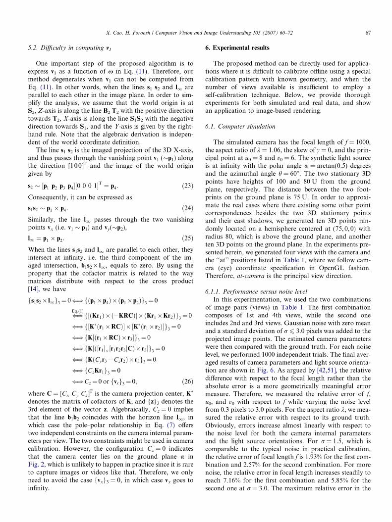
5.2. Difficulty in computing v1

One important step of the proposed algorithm is toexpress v1 as a function of x in Eq. (11). Therefore, ourmethod degenerates when v1 can not be computed fromEq. (11). In other words, when the lines s1 s2 and l1 areparallel to each other in the image plane. In order to sim-plify the analysis, we assume that the world origin is atS2, Z-axis is along the line B2 T2 with the positive directiontowards T2, X-axis is along the line S1S2 with the negativedirection towards S1, and the Y-axis is given by the right-hand rule. Note that the algebraic derivation is indepen-dent of the world coordinate definition.

The line s1 s2 is the imaged projection of the 3D X-axis,and thus passes through the vanishing point v1 (�p1) alongthe direction [10 0]T and the image of the world origingiven by

s2 � ½p1 p2 p3 p4�½0 0 0 1�T ¼ p4: ð23ÞConsequently, it can be expressed as

s1s2 � p1 � p4: ð24ÞSimilarly, the line l1 passes through the two vanishingpoints vx (i.e. v1 � p1) and vy(�p2),

l1 ¼ p1 � p2: ð25ÞWhen the lines s1s2 and l1 are parallel to each other, theyintersect at infinity, i.e. the third component of the im-aged intersection, b1s2 · l1, equals to zero. By using theproperty that the cofactor matrix is related to the waymatrices distribute with respect to the cross product[14], we have

fs1s2� l1g3¼ 0()fðp1�p4Þ�ðp1�p2Þg3¼ 0

()Eq:ð1Þf½ðKr1Þ�ð�KRCÞ��ðKr1�Kr2Þg3¼ 0

()f½K�ðr1�RCÞ�� ½K�ðr1� r2Þ�g3¼ 0

()fK½ðr1�RCÞ� r3�g3¼ 0

()fK½ð½r1��½r1r2r3�CÞ� r3�g3¼ 0

()fKðCyr3�Czr2Þ� r3g3¼ 0

()fCzKr1g3¼ 0

()Cz¼ 0 or fvxg3¼ 0; ð26Þ

where C = [Cx Cy Cz]T is the camera projection center, K*

denotes the matrix of cofactors of K, and {z}3 denotes the3rd element of the vector z. Algebraically, Cz = 0 impliesthat the line b1b2 coincides with the horizon line l1, inwhich case the pole–polar relationship in Eq. (7) offerstwo independent constraints on the camera internal param-eters per view. The two constraints might be used in cameracalibration. However, the configuration Cz = 0 indicatesthat the camera center lies on the ground plane p inFig. 2, which is unlikely to happen in practice since it is rareto capture images or videos like that. Therefore, we onlyneed to avoid the case {vx}3 = 0, in which case vx goes toinfinity.

6. Experimental results

The proposed method can be directly used for applica-tions where it is difficult to calibrate offline using a specialcalibration pattern with known geometry, and when thenumber of views available is insufficient to employ aself-calibration technique. Below, we provide thoroughexperiments for both simulated and real data, and showan application to image-based rendering.

6.1. Computer simulation

The simulated camera has the focal length of f = 1000,the aspect ratio of k = 1.06, the skew of c = 0, and the prin-cipal point at u0 = 8 and v0 = 6. The synthetic light sourceis at infinity with the polar angle / = arctan(0.5) degreesand the azimuthal angle h = 60�. The two stationary 3Dpoints have heights of 100 and 80 U from the groundplane, respectively. The distance between the two foot-prints on the ground plane is 75 U. In order to approxi-mate the real cases where there existing some other pointcorrespondences besides the two 3D stationary pointsand their cast shadows, we generated ten 3D points ran-domly located on a hemisphere centered at (75, 0,0) withradius 80, which is above the ground plane, and anotherten 3D points on the ground plane. In the experiments pre-sented herein, we generated four views with the camera andthe ‘‘at’’ positions listed in Table 1, where we follow cam-era (eye) coordinate specification in OpenGL fashion.Therefore, at-camera is the principal view direction.

6.1.1. Performance versus noise level

In this experimentation, we used the two combinationsof image pairs (views) in Table 1. The first combinationcomposes of 1st and 4th views, while the second oneincludes 2nd and 3rd views. Gaussian noise with zero meanand a standard deviation of r 6 3.0 pixels was added to theprojected image points. The estimated camera parameterswere then compared with the ground truth. For each noiselevel, we performed 1000 independent trials. The final aver-aged results of camera parameters and light source orienta-tion are shown in Fig. 6. As argued by [42,51], the relativedifference with respect to the focal length rather than theabsolute error is a more geometrically meaningful errormeasure. Therefore, we measured the relative error of f,u0, and v0 with respect to f while varying the noise levelfrom 0.3 pixels to 3.0 pixels. For the aspect ratio k, we mea-sured the relative error with respect to its ground truth.Obviously, errors increase almost linearly with respect tothe noise level for both the camera internal parametersand the light source orientations. For r = 1.5, which iscomparable to the typical noise in practical calibration,the relative error of focal length f is 1.93% for the first com-bination and 2.57% for the second combination. For morenoise, the relative error in focal length increases steadily toreach 7.16% for the first combination and 5.85% for thesecond one at r = 3.0. The maximum relative error in the

Table 1External parameters of four different viewpoints

View 1st 2nd 3rd 4th

Camera position (10,�100,40) (�150,�100,40) (10,�100,100) (�150,�100,100)‘‘at’’ position (�100,0,0) (�100,0, 0) (�100,0,0) (�100,0,0)

0 1 2 30

0.02

0.04

0.06

0.08

Noise Level (pixels)

Rel

ativ

e E

rror

using 1st and 4th views

using 2nd and 3rd views

0 1 2 30

0.02

0.04

0.06

0.08

0.1

0.12

0.14

Noise Level (pixels)R

elat

ive

Err

or



focal length aspect ratio

0 1 2 30

0.01

0.02

0.03

0.04

0.05

0.06

0.07


Rel

ativ

e E

rror



0 1 2 30

0.02

0.04

0.06

0.08

0.1


Rel

ativ

e E

rror



of principal point of principal point

0 1 2 30

0.5

1

1.5

2

2.5


Abs

olut

e E

rror



0 1 2 30

0.5

1

1.5

2

2.5


Abs

olut

e E

rror



Polar angle Azimuthal angle

Fig. 6. The performance of our method under different noise levels (in pixels).


aspect ratio is 13.96% for the first combination, and 5.22%for the second combination. The maximum relative errorsin the coordinates of the principal point are around

6.51% for u0 and about 9.74% for v0. Finally, the computedorientation of the light source is within ±2.5� for bothpolar and azimuthal angles.


6.1.2. Performance versus the orientation of the image plane

Another experiment performed was to examine theinfluence of the relative orientation between the verticalplane p1 (see Fig. 2) and the image plane. Two views wereused. The orientation of the image planes of two views werechosen as follows: the image planes were initially parallel tothe vertical plane; a rotation axis was randomly chosenfrom a uniform sphere; the image planes were then rotatedaround that axis with angle w. Considering the fact thatextracted feature points will in practice be affected by noise,we also added a typical noise level of r = 1.0 pixels to allprojected image points. We repeated this process 1000times and computed the average errors. The angle w is var-ied from 5� to 85�, and the results are shown in Fig. 7. Sev-eral important observations are made immediately. First,the results validate the partial analysis of degenerate casesin Section 5.1. In case (i) where the image plane is parallelto the vertical plane, i.e. w = 0�, our method degenerates.In case (iii), i.e. w = 90�, our method is also degenerate,but is able to recover the principal point since in our exper-iments the image planes of both views are also approxi-mately perpendicular to the ground plane. The secondobservation is that the best performance seems to beachieved with an angle around 45�. Third, the minima ofthe curve is sufficiently broad so that in practice acceptableresults can be found from a wide range of viewing angles.Note that, when w increases, foreshortening makes the fea-ture detection less accurate, which is not considered inthese experiments.

6.1.3. Performance versus orthogonality errors

This last experiment was carried out to evaluate howsensitive the algorithm is to errors in estimating the foot-prints bi, which enforce the fact that tibi must be orthogo-nal to the ground plane. For each direction tibi, we addedindependent Gaussian noise with zero mean and a standarddeviation of r 6 3.0�. Considering the fact that the extract-ed feature points will in practice be affected by noise, we alsoadded a typical noise level of r = 1.0 pixels to all projectedimage points. We repeated this process 1000 times, and thefinal averaged results of camera parameters and light sourceorientation are shown in Fig. 8. The errors in both cameraparameters and light source orientation increase almost

0 20 40 60 800

0.2

0.4

0.6

0.8

1

1.2

Relative Orientation (degrees)

Rel

ativ

e E

rror

focal lengthaspect ratio

0 20 400

0.5

1

1.5

2

Relative Orie

Rel

ativ

e E

rror

Fig. 7. The performance of our method with respect to the relativ

linearly with respect to the orthogonality errors. Notice thatthe errors do not go to zero as orthogonality errors tendtowards zero due to the added noise in image projections.For example, the relative errors of focal lengths are around1.8% under orthogonality error r = 0.3� and pixel noiser = 1.0 pixels (Fig. 8 top left), while the focal length errorsare around 1.4% when there is same pixel noise r = 1.0pixels but no orthogonality error (Fig. 6 top left).

6.2. Real data

We also applied our method to real images. The firstimage set consisted of three views of a standing personand a lamp (see Fig. 9). For each pair of images, we appliedour algorithm independently, and the results are shown inTable 2. In order to evaluate our results, we used themethod in [23] to obtain an over-determined least-squaressolution for our camera internal parameters from the noisymeasurements. Results from this method are listed in thelast column of Table 2 as the ground truth for comparison.The largest relative error in the focal length, in our method,is less than 4.5%. The maximum relative error of principalpoint is around 5.4%. In addition, the computed polarangle / and the azimuthal angle h are 44.54� and 33.22�,respectively, while they are 45.09� and 32.97� by usingthe intrinsic parameters in the last column of Table 2. Toverify how these constraints can be used to increase theoverall accuracy when more images are used, we appliedour method on all the three views and compared with theground truth as shown in Table 2. As expected, the moreimages are used, the better is the performance. The errorscould be attributed to several sources. Besides noise, non-linear distortion, and errors in the extracted features, onesource is the casual experimental setup using minimalinformation, which is deliberately targeted to demonstratea wide spectrum of applications. Despite all these factors,our experimentations indicate that the proposed algorithmprovides good results.

6.3. Application to image-based rendering

To demonstrate the strength and the utility of the pro-posed algorithm, we show two examples for augmented

60 80

ntation (degrees)

u0

v0

0 20 40 60 800

5

10

15

20

25

30

Relative Orientation (degrees)

Abs

olut

e E

rror

(de

gree

s) Polar angleAzimuthal angle

e orientation between the vertical plane and the image plane.

0 1 2 30

0.02

0.04

0.06

0.08

0.1

0.12

Orthognoal Errors (degrees)

Rel

ativ

e E

rror

using 1st and 4th viewsusing 2nd and 3rd views

0 1 2 30

0.02

0.04

0.06

0.08

0.1


Rel

ativ

e E

rror


0 1 2 30

0.02

0.04

0.06

0.08

0.1

0.12

0.14


Rel

ativ

e E

rror


focal length aspect ratio of principal point

0 1 2 30

0.05

0.1

0.15

0.2


Rel

ativ

e E

rror


0 1 2 30.5

1

1.5

2

2.5


Abs

olut

e E

rror

(de

gree

s) using 1st and 4th viewsusing 2nd and 3rd views

0 1 2 30

0.5

1

1.5

2


Abs

olut

e E

rror

(de

gree

s) using 1st and 4th viewsusing 2nd and 3rd views

of principal point Polar angle Azimuthal angle

Fig. 8. The performance of our method with respect to the orthogonality errors. The orthogonality errors here refer to errors in estimating the footprintsbi, which enforce the constraint that tibi must be orthogonal to the ground plane.

Fig. 9. Three images of a standing person and a lamp. The circle marks in the images are the minimal data computed by the method described in Section 4.

Table 2Calibration results for the first real image set

Relative error Test images [23]

(1,2) (1,3) (2,3) (1–3)

f 3200.8 (1.44%) 3137.1 (�0.58%) 3211.1 (1.77%) 3173.2 (0.57%) 3155.3kf 3206.1 (�3.21%) 3171.0 (�4.27%) 3216.4 (�2.90%) 3267.8 (�1.35%) 3312.5u0 1172.4 (0.28%) 1334.9 (5.43%) 1170.1 (0.21%) 1168.2 (0.15%) 1163.6v0 895.8 (�0.57%) 902.7 (�0.35%) 901.5 (�0.39%) 906.1 (�0.24%) 913.8


reality by making use of the camera and light source orien-tation information computed by our method. Given twoviews as shown in Fig. 10a and b, the computed K is

K ¼2641:11 0 991:70

0 2783:97 642:28

0 0 1

264

375;

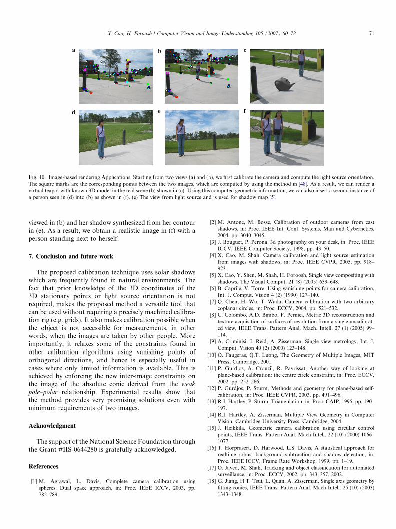
and the computed polar angle / and azimuthal angle h are47.99� and 54.91�, respectively. As a result, we can render avirtual teapot with known 3D model in the real scene (b) asshown in (c), where the color characteristics are estimatedusing the method presented in [5]. Alternatively, we canalso follow the method presented in [5] to composite thestanding person extracted from (d) with the same person

a b c

d e f

Fig. 10. Image-based rendering Applications. Starting from two views (a) and (b), we first calibrate the camera and compute the light source orientation.The square marks are the corresponding points between the two images, which are computed by using the method in [48]. As a result, we can render avirtual teapot with known 3D model in the real scene (b) shown in (c). Using this computed geometric information, we can also insert a second instance ofa person seen in (d) into (b) as shown in (f). (e) The view from light source and is used for shadow map [5].


viewed in (b) and her shadow synthesized from her contourin (e). As a result, we obtain a realistic image in (f) with aperson standing next to herself.

7. Conclusion and future work

The proposed calibration technique uses solar shadowswhich are frequently found in natural environments. Thefact that prior knowledge of the 3D coordinates of the3D stationary points or light source orientation is notrequired, makes the proposed method a versatile tool thatcan be used without requiring a precisely machined calibra-tion rig (e.g. grids). It also makes calibration possible whenthe object is not accessible for measurements, in otherwords, when the images are taken by other people. Moreimportantly, it relaxes some of the constraints found inother calibration algorithms using vanishing points oforthogonal directions, and hence is especially useful incases where only limited information is available. This isachieved by enforcing the new inter-image constraints onthe image of the absolute conic derived from the weak

pole–polar relationship. Experimental results show thatthe method provides very promising solutions even withminimum requirements of two images.

Acknowledgment

The support of the National Science Foundation throughthe Grant #IIS-0644280 is gratefully acknowledged.

References

[1] M. Agrawal, L. Davis, Complete camera calibration usingspheres: Dual space approach, in: Proc. IEEE ICCV, 2003, pp.782–789.

[2] M. Antone, M. Bosse, Calibration of outdoor cameras from castshadows, in: Proc. IEEE Int. Conf. Systems, Man and Cybernetics,2004, pp. 3040–3045.

[3] J. Bouguet, P. Perona. 3d photography on your desk, in: Proc. IEEEICCV, IEEE Computer Society, 1998, pp. 43–50.

[4] X. Cao, M. Shah. Camera calibration and light source estimationfrom images with shadows, in: Proc. IEEE CVPR, 2005, pp. 918–923.

[5] X. Cao, Y. Shen, M. Shah, H. Foroosh, Single view compositing withshadows, The Visual Comput. 21 (8) (2005) 639–648.

[6] B. Caprile, V. Torre, Using vanishing points for camera calibration,Int. J. Comput. Vision 4 (2) (1990) 127–140.

[7] Q. Chen, H. Wu, T. Wada, Camera calibration with two arbitrarycoplanar circles, in: Proc. ECCV, 2004, pp. 521–532.

[8] C. Colombo, A.D. Bimbo, F. Pernici, Metric 3D reconstruction andtexture acquisition of surfaces of revolution from a single uncalibrat-ed view, IEEE Trans. Pattern Anal. Mach. Intell. 27 (1) (2005) 99–114.

[9] A. Criminisi, I. Reid, A. Zisserman, Single view metrology, Int. J.Comput. Vision 40 (2) (2000) 123–148.

[10] O. Faugeras, Q.T. Luong, The Geometry of Multiple Images, MITPress, Cambridge, 2001.

[11] P. Gurdjos, A. Crouzil, R. Payrissat, Another way of looking atplane-based calibration: the centre circle constraint, in: Proc. ECCV,2002, pp. 252–266.

[12] P. Gurdjos, P. Sturm, Methods and geometry for plane-based self-calibration, in: Proc. IEEE CVPR, 2003, pp. 491–496.

[13] R.I. Hartley, P. Sturm, Triangulation, in: Proc. CAIP, 1995, pp. 190–197.

[14] R.I. Hartley, A. Zisserman, Multiple View Geometry in ComputerVision, Cambridge University Press, Cambridge, 2004.

[15] J. Heikkila, Geometric camera calibration using circular controlpoints, IEEE Trans. Pattern Anal. Mach Intell. 22 (10) (2000) 1066–1077.

[16] T. Horprasert, D. Harwood, L.S. Davis, A statistical approach forrealtime robust background subtraction and shadow detection, in:Proc. IEEE ICCV, Frame Rate Workshop, 1999, pp. 1–19.

[17] O. Javed, M. Shah, Tracking and object classification for automatedsurveillance, in: Proc. ECCV, 2002, pp. 343–357, 2002.

[18] G. Jiang, H.T. Tsui, L. Quan, A. Zisserman, Single axis geometry byfitting conies, IEEE Trans. Pattern Anal. Mach Intell. 25 (10) (2003)1343–1348.


[19] S. Kang, R.S. Weiss, Can we calibrate a camera using an image of aflat, textureless lambertian surface? in: Proc. ECCV, 2000, pp. 640–653.

[20] A. Klaus, J. Bauer, K. Karner, P. Elbischger, R. Perko, H. Bischof,Camera calibration from a single night sky image, in: Proc. IEEECVPR, 2004, pp. 151–157.

[21] N. Krahnstoever, P.R.S. Mendonca, Bayesian autocalibration forsurveillance, in: Proc. IEEE ICCV, 2005, pp. 1858–1865.

[22] D. Kriegman, P. Belhumeur, What shadows reveal about objectstructure, in: Proc. ECCV, 1998, pp. 399–414.

[23] D. Liebowitz, A. Zisserman, Combining scene and auto-calibrationconstraints, in: Proc. IEEE ICCV, 1999, pp. 293–300.

[24] C. Lin, A. Huertas, R. Nevatia, Detection of buildings usingperceptual groupings and shadows, 1994, 62–69.

[25] F. Lv, T. Zhao, R. Nevatia, Self-calibration of a camera from video ofa walking human, in: Proc. ICPR, 2002, pp. 562–567.

[26] E. Malis, R. Cipolla, Camera self-calibration from unknownplanar structures enforcing the multi-view constraints betweencollineations, IEEE Trans. Pattern Anal. Mach. Intell. 24 (9)(2002) 1268–1272.

[27] P.R.S. Mendonca, Multiview Geometry: Profiles and Self-Calibra-tion. Ph.D. thesis, University of Cambridge, Cambridge, UK, May2001.

[28] X. Meng, Z. Hu, A new easy camera calibration technique based oncircular points, Pattern Recogn. 36 (5) (2003) 1155–1164.

[29] I. Mikic, P. Cosman, G. Kogut, M. Trivedi, Moving shadow andobject detection in traffic scenes, in: Proc. ICPR, vol. 1, 2000,pp. 321–324.

[30] S. Nadimi, B. Bhanu, Physical models for moving shadow and objectdetection in video, IEEE Trans. Pattern Anal. Mach. Intell. 26 (8)(2004) 1079–1087.

[31] T. Okabe, I. Sato, Y. Sato, Spherical harmonics vs. haarwavelets:basis for recovering illumination from cast shadows, in: IEEEConference on CVPR, 2004, pp. 50–57.

[32] L. Petrovic, B. Fujito, L. Williams, A. Finkelstein, Shadows for celanimation, in: Proc. ACM SIGGRAPH, 2000, pp. 511–516.

[33] M. Pollefeys, R. Koch, L.V. Gool, Self-calibration and metricreconstruction in spite of varying and unknown internal cameraparameters, Int. J. Comput. Vision 32 (1) (1999) 7–25.

[34] A. Prati, I. Mikic, M. Trivedi, R. Cucchiara, Detecting movingshadows: algorithms and evaluation, IEEE Trans. Pattern Anal.Mach. Intell. 25 (7) (2003) 918–923.

[35] W. Press, B. Flannery, S. Teukolsky, W. Vetterling, NumericalRecipes in C, Cambridge University Press, Cambridge, 1988.

[36] I. Reid, A. North,3D trajectories from a single viewpoint usingshadows, in: Proc. of BMVC, 1998.

[37] I. Sato, Y. Sato, K. Ikeuchi, Illumination from shadows, IEEE Trans.Pattern Anal. Mach Intell. 25 (3) (2003) 290–300.

[38] S. Sinha, M. Pollefeys, L. McMillan, Camera network calibrationfrom dynamic silhouettes, in: Proc. IEEE CVPR, 2005, pp. 195–202.

[39] J. Stauder, R. Mech, J. Ostermann, Detection of moving cast shadowsfor object segmentation, IEEE Trans. Multimedia 1 (1) (1999) 65–76.

[40] P. Sturm, S. Maybank, On plane-based camera calibration: a generalalgorithm, singularities, applications, in: Proc. IEEE CVPR, 1999, pp.432–437.

[41] H. Teramoto and G. Xu. Camera calibration by a single image ofballs: from conic to the absolute conic, in: Proc. ACCV, 2002, pp.499–506.

[42] B. Triggs, Autocalibration from planar scenes, in: Proc. ECCV, 1998,pp. 89–105.

[43] B. Triggs, P. McLauchlan, R.I. Hartley, A. Fitzgibbon, Bundleadjustment—a modern synthesis, in: Vision Algorithms: Theory andPractice, 1999, pp. 298–373.

[44] R.Y. Tsai, A versatile camera calibration technique for high-accuracy3D machine vision metrology using off-the-shelf tv cameras andlenses, IEEE J. Robotics Autom. 3 (4) (1987) 323–344.

[45] L. Van Gool, M. Proesmans, A. Zisserman, Planar homologies as abasis for grouping and recognition, Image Vision Comput. 16 (1998)21–26.

[46] K.-Y. Wong, R.S. P Mendonca, R. Cipolla, Camera calibration fromsurfaces of revolution, IEEE Trans. Pattern Anal. Mach Intell. 25 (2)(2003) 147–161.

[47] Y. Wu, H. Zhu, Z. Hu, F. Wu, Camera calibration from the quasi-affine invariance of two parallel circles, in: Proc. ECCV, 2004, pp.190–202.

[48] J. Xiao, M. Shah, Two-frame wide baseline matching, in: Proc. IEEEICCV, 2003, pp. 603–609.

[49] H. Zhang, G. Zhang, K.-Y.K. Wong, Camera calibration withspheres: linear approaches, in: Proc. IEEE ICIP, vol. II, 2005, pp.1150–1153.

[50] Z. Zhang, A flexible new technique for camera calibration, IEEETrans. Pattern Anal. Mach Intell. 22 (11) (2000) 1330–1334.

[51] Z. Zhang, Camera calibration with one-dimensional objects, IEEETrans. Pattern Anal. Mach Intell. 26 (7) (2004) 892–899.

camera calibration and light source orientation from solar...

Documents