23rd Computer Vision Winter WorkshopZuzana Kukelova and Julia Skovierova (eds.)Cesky Krumlov, Czech Republic, February 5–7, 2018

Camera-based vehicle velocity estimation from monocular video

Moritz Kampelmuhler1 Michael G. Muller2 Christoph Feichtenhofer1

1Institute of Electrical Measurement and Measurement Signal Processing2Institute of Theoretical Computer Science

Graz University of Technologykampelmuehler@student.tugraz.at, mueller@igi.tugraz.at, feichtenhofer@tugraz.at

Abstract. This paper documents the winning entry atthe CVPR2017 vehicle velocity estimation challenge.Velocity estimation is an emerging task in au-tonomous driving which has not yet been thoroughlyexplored. The goal is to estimate the relative veloc-ity of a specific vehicle from a sequence of images. Inthis paper, we present a light-weight approach for di-rectly regressing vehicle velocities from their trajec-tories using a multilayer perceptron. Another contri-bution is an explorative study of features for monoc-ular vehicle velocity estimation. We find that light-weight trajectory based features outperform depthand motion cues extracted from deep ConvNets, espe-cially for far-distance predictions where current dis-parity and optical flow estimators are challenged sig-nificantly. Our light-weight approach is real-time ca-pable on a single CPU and outperforms all compet-ing entries in the velocity estimation challenge. Onthe test set, we report an average error of 1.12 m/swhich is comparable to a (ground-truth) system thatcombines LiDAR and radar techniques to achieve anerror of around 0.71 m/s.

1. Introduction

Camera sensors provide an inexpensive yet pow-erful alternative to range sensors based on LiDAR orradar. While LiDAR systems can provide very accu-rate measurements, they may also malfunction underadverse environmental conditions such as fog, snow,rain or even exhaust gas fumes [30, 14]. Arguably vi-sion based sensing is more closely related to how hu-mans engage in driving situations and it should thusbe possible to solve any task in autonomous drivingbased on visual input.

This work addresses monocular vehicle velocityestimation, an emerging task in autonomous driving

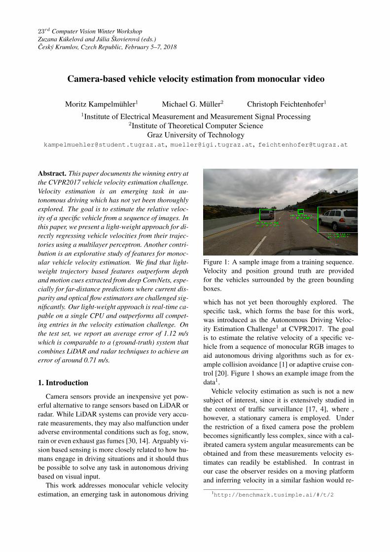
Figure 1: A sample image from a training sequence.Velocity and position ground truth are providedfor the vehicles surrounded by the green boundingboxes.

which has not yet been thoroughly explored. Thespecific task, which forms the base for this work,was introduced as the Autonomous Driving Veloc-ity Estimation Challenge1 at CVPR2017. The goalis to estimate the relative velocity of a specific ve-hicle from a sequence of monocular RGB images toaid autonomous driving algorithms such as for ex-ample collision avoidance [1] or adaptive cruise con-trol [20]. Figure 1 shows an example image from thedata1.

Vehicle velocity estimation as such is not a newsubject of interest, since it is extensively studied inthe context of traffic surveillance [17, 4], where ,however, a stationary camera is employed. Underthe restriction of a fixed camera pose the problembecomes significantly less complex, since with a cal-ibrated camera system angular measurements can beobtained and from these measurements velocity es-timates can readily be established. In contrast inour case the observer resides on a moving platformand inferring velocity in a similar fashion would re-

1http://benchmark.tusimple.ai/#/t/2

quire additional information such as camera pose,ego-motion and foreground-background segmenta-tion. Very recent research [41] shows that estimatingego-motion as well as disparity maps from monocu-lar camera images by means of structure from motionis indeed possible, but still limited. Semantic seg-mentation of scenes, which is a fundamental prob-lem in computer vision, has also more recently beentackled using deep neural networks [6, 24].

In a more general sense the given task can beseen as a lightweight version of object scene flowas for example provided in the KITTI benchmark[11, 28]. Object scene flow aims at estimating dense3D motion fields, which in their temporal evolutioncarry highly valuable information about the geomet-ric constellation of a given scene. Recent approaches[36, 35] yield impressive results, but they rely on theavailability of stereo image data. Furthermore, theycome at the price of very high computational cost,such that the estimation for a temporal frame pairmight take 5-10 minutes on a single CPU core. In au-tonomous driving scenarios computational resourcesare in general highly limited [13], which makes ob-ject scene flow currently not practically feasible.

In this work we adopt recent deep learning archi-tectures [18, 12] for depth and motion estimation toleverage a mapping of the video input into a bene-ficial feature space for learning from the few train-ing samples provided. Our approach employs a two-stage process for monocular velocity estimation. Ina first step we extract vehicle tracks as well as densedepth and optical flow information, followed by lo-cally aggregating these depth and motion cues at thetracked vehicle locations and concatenating over thetemporal dimension. After this feature extractionprocedure we use the spatiotemporal depth, flow andlocation features to train a fully connected regressionnetwork for velocity estimation of the respective ve-hicles.

Further on we conduct an extensive ablation studyto investigate the impact of the individual featuresand combinations thereof on the regression perfor-mance as well as on the runtime of the estimation.We show that a light weight implementation canachieve excellent results, and that leveraging deepmotion and depth cues does not necessarily improveperformance for this task on the given data.

2. Related Work

Tracking. Object tracking is one of the fundamen-tal problems in computer vision and has been ex-tensively studied [40] and applied in many differenttasks.

Median Flow [21] is a method building on top ofthe Lucas-Kanade [25] method, which is an earlyoptical flow algorithm operating on local intensitychanges. This method is extended by a Forward-Backward error, which denotes the deviation be-tween the trajectories obtained by tracking fromIt−1 → It and It → It−1. Using Forward-Backwarderror, robust predictions can be identified.

The Multiple Instance Learning tracker [2] firsttransforms the image into an appropriate featurespace, and uses a classifier as well as a motion modelto determine the presence of an object in a frame,which is referred to as tracking by detection.

More recent methods like [15] employ convolu-tional neural networks to learn motion and appear-ance of objects. The feature maps of higher convolu-tional layers provide robust and accurate appearancerepresentations, but lack spatial resolution. Lowerlayers on the other hand provide higher spatial res-olution and less refined appearance representations.This hierarchical structure is used in [26] by inferringresponses of correlation filters on each correspondinglayer pair.

Monocular Depth Estimation. Estimating thedepth information of a scene seen from a given an-gle using only a single camera is not a well-posedproblem. Some of the methods tackling this problem[31, 39] apply supervised learning regimes requiringground truth depth data. Since acquiring such groundtruth data with sufficient accuracy requires immenseeffort, several methods are being developed that re-quire little to no supervision.

In [23] a semi-supervised approach is describedthat provides a fusion between using sparse groundtruth data from a LiDAR sensor and stereo view syn-thesis, i.e. estimating one image in a stereo pair fromthe other, to infer dense depth maps. Others [12, 38]in turn rely solely on stereo as a supervision signal,which comes with the benefit of easily available orobtainable data.

Some recent work [41, 10] shows the capability ofinferring single image depth from monocular videoonly. This is achieved by leveraging the (small) tem-poral motion of the camera and its thus changingpose to learn from multiple views of the scene. Via

Tracker

FlowNet

DepthNet

RGB

Input frames

stack

Backward propagation

Forward propagation

pool

*

MLP

width

depth

height

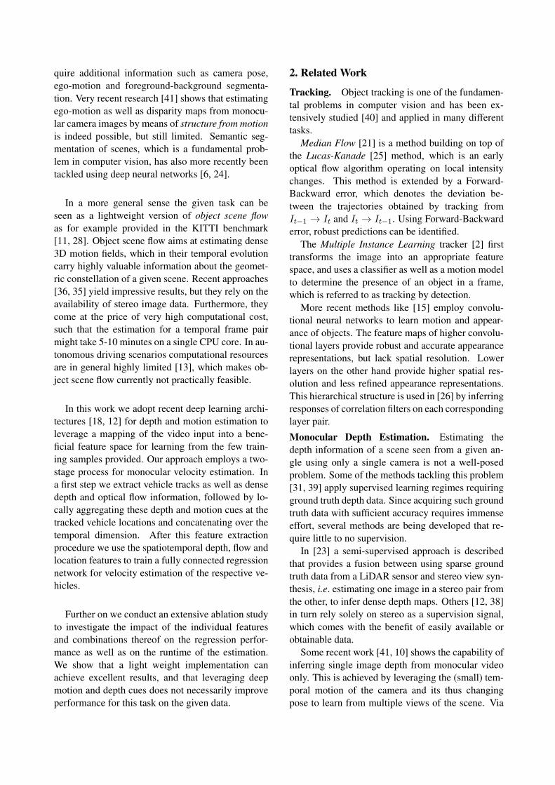
Figure 2: Overview of our overall architecture (see Section 3 for details). Our proposed light-weight architec-ture only uses the trajectory features estimated by the tracker.

novel view synthesis the future camera frames can beused as a self-supervision signal. The mapping thuslearned implicitly carries information about the 3Dscene geometry.

Optical Flow Estimation. Optical flow is widelyused in computer vision, e.g. for video object de-tection [42], to quantify pixel-wise motion in be-tween frames of a moving scene. Traditional meth-ods [16, 37] employ variational motion estimationapproaches, that regard the estimation of pixel levelcorrespondences between frames as an optimizationproblem.

With the growing interest in deep learning alsooptical flow estimation is now often successfullytreated as a supervised learning problem [7]. Thisis achieved by employing convolutional neural net-works for feature extraction and aggregation, fol-lowed by an ’upconvolutional’ network, which con-catenates the feature maps from the correspond-ing convolutional layers and jointly applies trans-posed convolution to increase spatial resolution. Fur-ther improvements on this approach have since beenmade [18] that provide improved performance androbustness as well as scalability.

3. Vehicle velocity estimation

We present an explorative study over features forvehicle velocity estimation from monocular cameravideos and discuss effectiveness as well as signifi-cance of the methods employed. The task is to esti-mate the relative velocity as well as position of givenvehicles seen in short dashcam video snippets. Ouroverall approach, shown in Figure 2, consists of atwo stage process: First, features subsidiary to the

task are extracted to subserve the second stage, whichis a light-weight Multilayer Perceptron (MLP) archi-tecture working on these features to regress velocityand positions of vehicle instances.

3.1. Feature Extraction

For the estimation of vehicle velocity, the rawRGB video data is first transformed into a beneficialfeature space. We use three feature types of com-plementary nature: Vehicle tracks (i.e. trajectories ofthe 2D object outline over time), depth (i.e. disparityestimates from monocular imagery) and motion (i.e.optical flow estimates between consecutive frames).The remainder of this section describes the specificalgorithmic instances used for extracting these cues.Tracks. For a given vehicle defined by a bound-ing box in a single frame, tracking over the temporalextent of the input serves for all further processingsteps. A variety of well functioning tracking algo-rithms are readily available in literature. Since weaim for a lightweight tracker that should preciselylocalize the object outline, we employ fast track-ers that operate directly at the pixel level, the Me-dian Flow [21] and MIL [2] trackers, both imple-mented in the OpenCV library [3]. The Median Flowtracker comes with the benefit of being able to adaptbounding boxes over the trajectories, and provides atight bounding box that can be a very useful featurewhen estimating the relative velocity of the objects.However, this tracker is unstable for occlusions sinceit employs forward-backward tracking. WheneverMedian Flow detects a tracking failure the missingbounding boxes are substituted with MIL tracks.Depth. For dense depth map prediction we em-ploy a recently described deep architecture [12], that

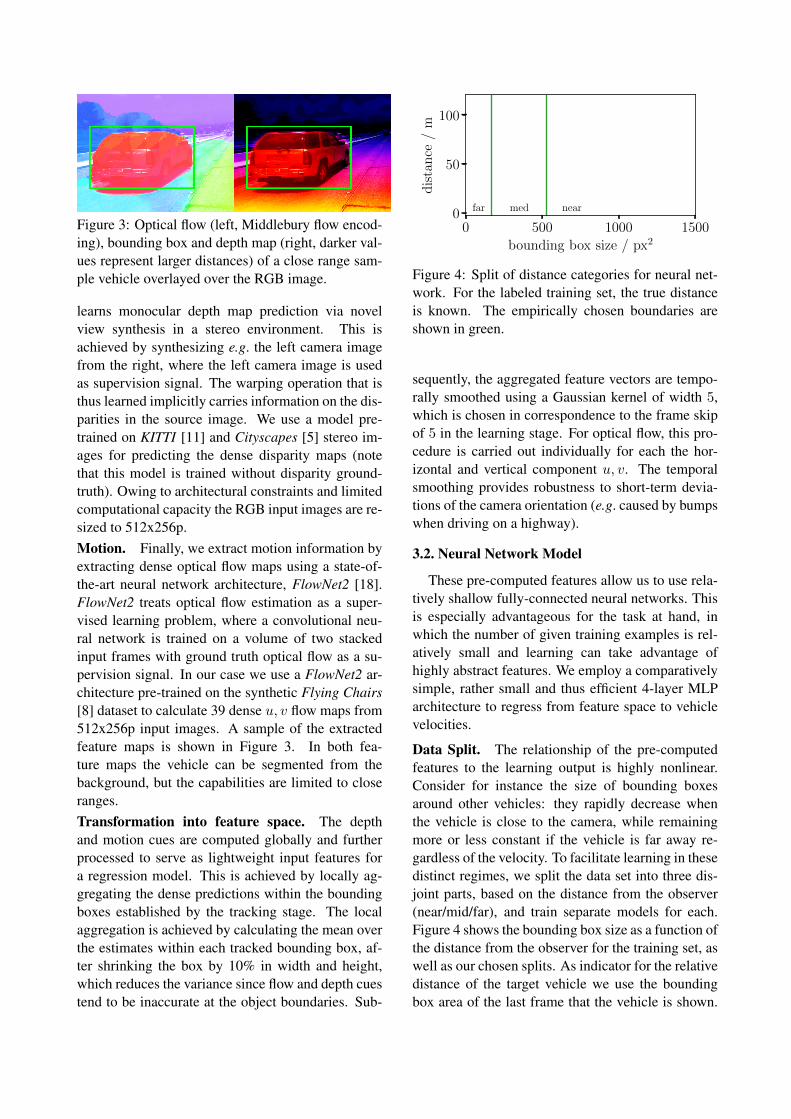
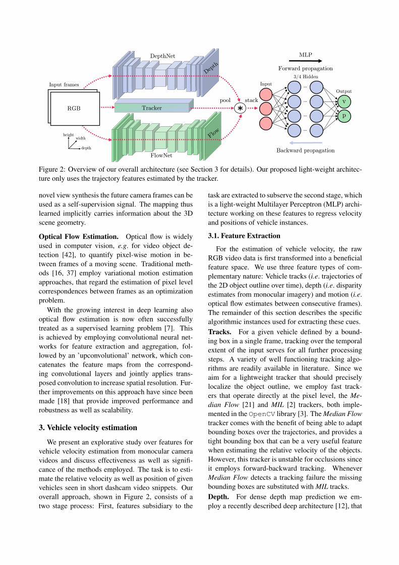
Figure 3: Optical flow (left, Middlebury flow encod-ing), bounding box and depth map (right, darker val-ues represent larger distances) of a close range sam-ple vehicle overlayed over the RGB image.

learns monocular depth map prediction via novelview synthesis in a stereo environment. This isachieved by synthesizing e.g. the left camera imagefrom the right, where the left camera image is usedas supervision signal. The warping operation that isthus learned implicitly carries information on the dis-parities in the source image. We use a model pre-trained on KITTI [11] and Cityscapes [5] stereo im-ages for predicting the dense disparity maps (notethat this model is trained without disparity ground-truth). Owing to architectural constraints and limitedcomputational capacity the RGB input images are re-sized to 512x256p.Motion. Finally, we extract motion information byextracting dense optical flow maps using a state-of-the-art neural network architecture, FlowNet2 [18].FlowNet2 treats optical flow estimation as a super-vised learning problem, where a convolutional neu-ral network is trained on a volume of two stackedinput frames with ground truth optical flow as a su-pervision signal. In our case we use a FlowNet2 ar-chitecture pre-trained on the synthetic Flying Chairs[8] dataset to calculate 39 dense u, v flow maps from512x256p input images. A sample of the extractedfeature maps is shown in Figure 3. In both fea-ture maps the vehicle can be segmented from thebackground, but the capabilities are limited to closeranges.Transformation into feature space. The depthand motion cues are computed globally and furtherprocessed to serve as lightweight input features fora regression model. This is achieved by locally ag-gregating the dense predictions within the boundingboxes established by the tracking stage. The localaggregation is achieved by calculating the mean overthe estimates within each tracked bounding box, af-ter shrinking the box by 10% in width and height,which reduces the variance since flow and depth cuestend to be inaccurate at the object boundaries. Sub-

0 500 1000 1500

bounding box size / px2

0

50

100

dis

tan

ce/

m

far med near

Figure 4: Split of distance categories for neural net-work. For the labeled training set, the true distanceis known. The empirically chosen boundaries areshown in green.

sequently, the aggregated feature vectors are tempo-rally smoothed using a Gaussian kernel of width 5,which is chosen in correspondence to the frame skipof 5 in the learning stage. For optical flow, this pro-cedure is carried out individually for each the hor-izontal and vertical component u, v. The temporalsmoothing provides robustness to short-term devia-tions of the camera orientation (e.g. caused by bumpswhen driving on a highway).

3.2. Neural Network Model

These pre-computed features allow us to use rela-tively shallow fully-connected neural networks. Thisis especially advantageous for the task at hand, inwhich the number of given training examples is rel-atively small and learning can take advantage ofhighly abstract features. We employ a comparativelysimple, rather small and thus efficient 4-layer MLParchitecture to regress from feature space to vehiclevelocities.

Data Split. The relationship of the pre-computedfeatures to the learning output is highly nonlinear.Consider for instance the size of bounding boxesaround other vehicles: they rapidly decrease whenthe vehicle is close to the camera, while remainingmore or less constant if the vehicle is far away re-gardless of the velocity. To facilitate learning in thesedistinct regimes, we split the data set into three dis-joint parts, based on the distance from the observer(near/mid/far), and train separate models for each.Figure 4 shows the bounding box size as a function ofthe distance from the observer for the training set, aswell as our chosen splits. As indicator for the relativedistance of the target vehicle we use the boundingbox area of the last frame that the vehicle is shown.

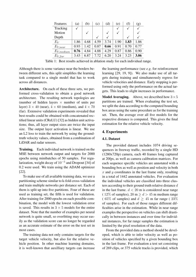
Features (a) (b) (c) (d) (e) (f) (g)Tracking X X X XMotion X X X XDepth X X X XEV 1.86 4.68 4.59 3.74 1.90 1.83 1.86EV,near 0.93 1.42 0.87 0.66 0.91 0.70 0.77EV,medium 0.76 4.84 4.88 4.29 0.87 0.86 0.90EV,far 3.43 6.87 7.72 6.20 3.24 3.23 3.06

Table 1: Best results achieved in ablation study for each individual range.

Although there is some variance near the borders be-tween different sets, this split simplifies the learningtask compared to a single model that has to workacross all distances.

Architecture. On each of these three sets, we per-formed cross-validation to obtain a good networkarchitecture. The resulting network topologies are(number of hidden layers × number of units perlayer) 3 × 40 (near), 4 × 60 (medium), and 4 × 70(far). Extensive validation experiments revealed thatbest results could be obtained with concatenated rec-tified linear units (CReLU) [32] as hidden unit activa-tions; thus, all layer output sizes are twice the inputsize. The output layer activation is linear. We usean L2 loss to train the network by using the ground-truth velocity values, obtained from a combination ofLiDAR and radar sensors.

Training. Each individual network is trained on theMSE between network output and targets for 2000epochs using minibatches of 50 samples. For regu-larization, weight decay of 10−5 and Dropout [34] of0.2 were used. We train using the ADAM optimizer[22].

To make use of all available training data, we use apartitioning scheme similar to k-fold cross-validationand train multiple networks per distance set. Each ofthem is split up into five partitions. Four of these areused as training set, the fifth is used for validation.After training for 2000 epochs on each possible com-bination, the model with the lowest validation erroris saved. This results in 3 × 5 models for the entiredataset. Note that the number of examples per neuralnetwork is quite small, so overfitting may occur eas-ily as the validation score can no longer be regardedas an accurate estimate of the error on the test set inmost cases.

The training data not only contains targets for thetarget vehicle velocity, but also for the relative ve-hicle position. In other machine learning domains,it is well-known that auxilliary targets can increase

the learning performance (see e.g. for reinforcementlearning [29, 19, 9]). We also make use of all tar-gets during training and simultaneously regress forvehicle velocities and distance. Early stopping is per-formed using only the performance on the actual tar-gets. This leads to slight increases in performance.

Model Averaging. Above, we described how 3×5partitions are trained. When evaluating the test set,we split the data according to the computed boundingbox areas using the same procedure as for the trainingset. Then, the average over all five models for therespective distance is computed. This gives the finalestimation for the relative vehicle velocity.

4. Experiments

4.1. Dataset

The provided dataset includes 1074 driving se-quences in freeway traffic, recorded by a single HD(1280x720p) camera, each 40 frames long capturedat 20fps, as well as camera calibration matrices. Foreach sequence specific vehicles are annotated with abounding box as well as position and velocity in bothx and y coordinates in the last frame only, resultingin a total of 1442 annotated vehicles. For evaluationthe individual vehicles are classified into three clus-ters according to their ground truth relative distance din the last frame. d < 20 m is considered near range( 12% of samples), 20 m ≥ d > 45 m medium range( 65% of samples) and d ≥ 45 m far range ( 23%of samples). For each of those ranges different dif-ficulties arise in the estimation. While in near rangeexamples the perspective on vehicles can shift drasti-cally in between instances and over time for individ-ual instances, for far range samples the estimation islimited by the pixel resolution of the data.

From the provided data a method should be devel-oped, which is able to infer velocity as well as po-sition of vehicles specified by a given bounding boxin the last frame. For evaluation a test set consistingof 269 clips, or 375 vehicle tracks is provided, which

is structurally identical to the training data, with theonly difference being the absence of ground truth po-sition and velocity data.

4.2. Ablation study

To investigate the impact of the features used inour initial approach on velocity estimation accuracy,we have conducted an ablation study to test combi-nations of all features and activation functions.

Validation split. In order to be able to evaluate theperformance of our approach we had to first split theavailable training data into a training and validationset. Earlier we used 80/20 random splits, but formore robust evaluation we decided to take into ac-count the distribution of near, medium and far rangesamples (12/65/23%) and also the similarity of thetest sequences. Since the training samples are se-quences from a fixed set of drives, we decided to splittraining and validation splits such that the validationsamples stem from unseen drives.

To achieve this we compute the 4096 dimensionalVGGNet fc2 feature vector [33], reduce it to 2D spaceusing t-sne [27] and then cluster the resulting featuresinto 7 clusters using k-means. We have then cho-sen a cluster consisting of 10% of the total trainingsamples with a (14/63/21%) near, medium, far rangedistribution as validation set. The remaining data isused for training after defining a fixed 5-fold split forcross validation.

Training. For each of the 5 train/test splits, 10models with fixed 3 × 40 topologies are trained ac-cording to the same paradigm as described above.Here, training was stopped early if the velocity meansquared error (1) did not improve in the course of 500iterations. The ablation was performed both trainingmodels on the whole data as well as training individ-ual models on near, medium and far data splits.

Results. The results of the ablation study describedabove are shown in Table 1. It can be seen that depthand motion cues can indeed help improve results ofvehicle velocity estimation, but their impact is lim-ited by range. Both depth and optical flow estimatesshow significantly degrading performances for dis-tances larger than 20m (above near range). Withinnear range on the other hand, where rapid changesin perspective can occur, they are superior in perfor-mance to using only tracking.

For medium range, where vehicles are predomi-nantly viewed from their rear only, tracking cues onlyyield superior performance. For far range the pixel

level appearance of vehicles changes so slightly atdifferent velocities, that a robust estimation of theirvelocity can not be achieved by the method used.

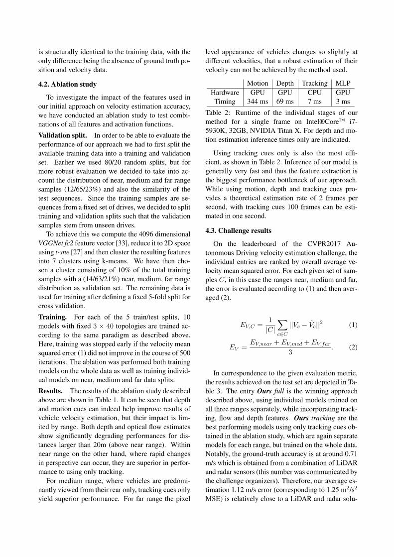
Motion Depth Tracking MLPHardware GPU GPU CPU GPU

Timing 344 ms 69 ms 7 ms 3 ms

Table 2: Runtime of the individual stages of ourmethod for a single frame on Intel®CoreTM i7-5930K, 32GB, NVIDIA Titan X. For depth and mo-tion estimation inference times only are indicated.

Using tracking cues only is also the most effi-cient, as shown in Table 2. Inference of our model isgenerally very fast and thus the feature extraction isthe biggest performance bottleneck of our approach.While using motion, depth and tracking cues pro-vides a theoretical estimation rate of 2 frames persecond, with tracking cues 100 frames can be esti-mated in one second.

4.3. Challenge results

On the leaderboard of the CVPR2017 Au-tonomous Driving velocity estimation challenge, theindividual entries are ranked by overall average ve-locity mean squared error. For each given set of sam-ples C, in this case the ranges near, medium and far,the error is evaluated according to (1) and then aver-aged (2).

EV,C =1

|C|∑c∈C||Vc − Vc||2 (1)

EV =EV,near + EV,med + EV,far

3. (2)

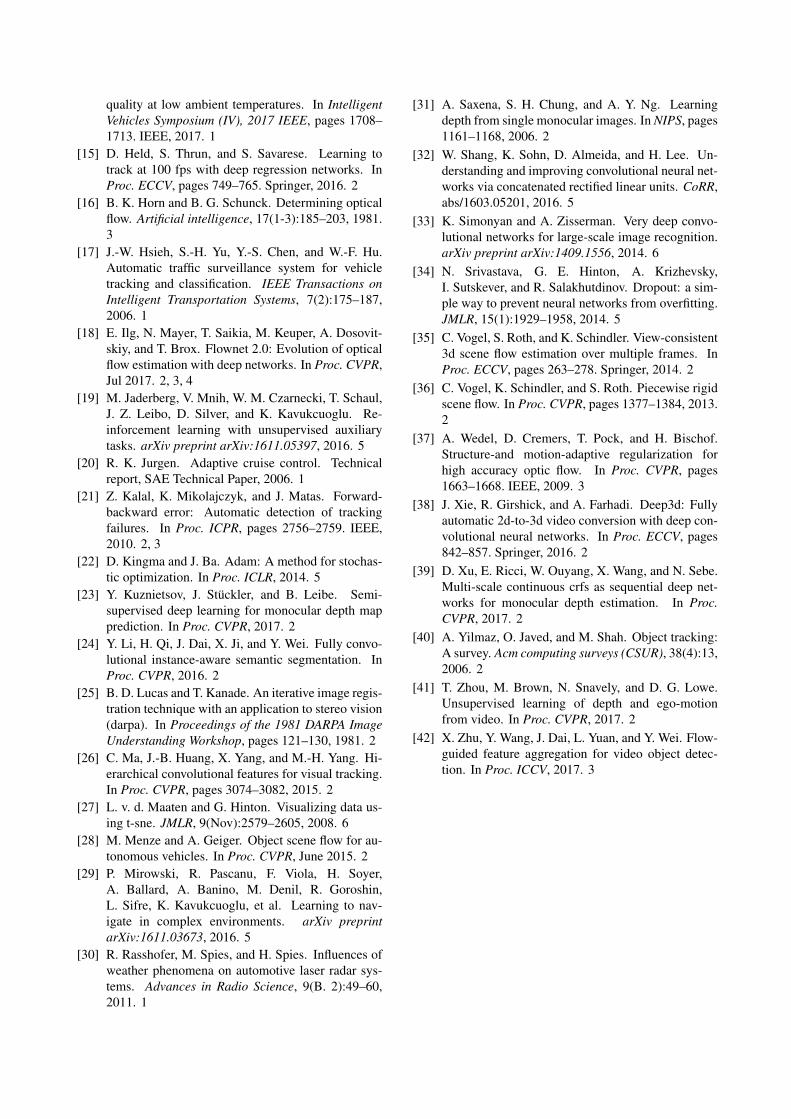
In correspondence to the given evaluation metric,the results achieved on the test set are depicted in Ta-ble 3. The entry Ours full is the winning approachdescribed above, using individual models trained onall three ranges separately, while incorporating track-ing, flow and depth features. Ours tracking are thebest performing models using only tracking cues ob-tained in the ablation study, which are again separatemodels for each range, but trained on the whole data.Notably, the ground-truth accuracy is at around 0.71m/s which is obtained from a combination of LiDARand radar sensors (this number was communicated bythe challenge organizers). Therefore, our average es-timation 1.12 m/s error (corresponding to 1.25 m2/s2

MSE) is relatively close to a LiDAR and radar solu-

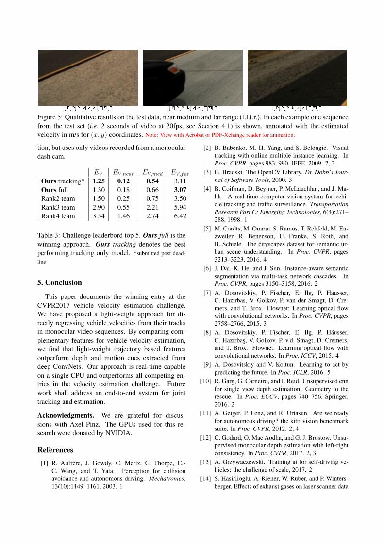
Figure 5: Qualitative results on the test data, near medium and far range (f.l.t.r.). In each example one sequencefrom the test set (i.e. 2 seconds of video at 20fps, see Section 4.1) is shown, annotated with the estimatedvelocity in m/s for (x, y) coordinates. Note: View with Acrobat or PDF-Xchange reader for animation.

tion, but uses only videos recorded from a monoculardash cam.

EV EV,near EV,med EV,far

Ours tracking* 1.25 0.12 0.54 3.11Ours full 1.30 0.18 0.66 3.07Rank2 team 1.50 0.25 0.75 3.50Rank3 team 2.90 0.55 2.21 5.94Rank4 team 3.54 1.46 2.74 6.42

Table 3: Challenge leaderbord top 5. Ours full is thewinning approach. Ours tracking denotes the bestperforming tracking only model. *submitted post dead-

line

5. Conclusion

This paper documents the winning entry at theCVPR2017 vehicle velocity estimation challenge.We have proposed a light-weight approach for di-rectly regressing vehicle velocities from their tracksin monocular video sequences. By comparing com-plementary features for vehicle velocity estimation,we find that light-weight trajectory based featuresoutperform depth and motion cues extracted fromdeep ConvNets. Our approach is real-time capableon a single CPU and outperforms all competing en-tries in the velocity estimation challenge. Futurework shall address an end-to-end system for jointtracking and estimation.

Acknowledgments. We are grateful for discus-sions with Axel Pinz. The GPUs used for this re-search were donated by NVIDIA.

References

[1] R. Aufrere, J. Gowdy, C. Mertz, C. Thorpe, C.-C. Wang, and T. Yata. Perception for collisionavoidance and autonomous driving. Mechatronics,13(10):1149–1161, 2003. 1

[2] B. Babenko, M.-H. Yang, and S. Belongie. Visualtracking with online multiple instance learning. InProc. CVPR, pages 983–990. IEEE, 2009. 2, 3

[3] G. Bradski. The OpenCV Library. Dr. Dobb’s Jour-nal of Software Tools, 2000. 3

[4] B. Coifman, D. Beymer, P. McLauchlan, and J. Ma-lik. A real-time computer vision system for vehi-cle tracking and traffic surveillance. TransportationResearch Part C: Emerging Technologies, 6(4):271–288, 1998. 1

[5] M. Cordts, M. Omran, S. Ramos, T. Rehfeld, M. En-zweiler, R. Benenson, U. Franke, S. Roth, andB. Schiele. The cityscapes dataset for semantic ur-ban scene understanding. In Proc. CVPR, pages3213–3223, 2016. 4

[6] J. Dai, K. He, and J. Sun. Instance-aware semanticsegmentation via multi-task network cascades. InProc. CVPR, pages 3150–3158, 2016. 2

[7] A. Dosovitskiy, P. Fischer, E. Ilg, P. Hausser,C. Hazirbas, V. Golkov, P. van der Smagt, D. Cre-mers, and T. Brox. Flownet: Learning optical flowwith convolutional networks. In Proc. CVPR, pages2758–2766, 2015. 3

[8] A. Dosovitskiy, P. Fischer, E. Ilg, P. Hausser,C. Hazırbas, V. Golkov, P. v.d. Smagt, D. Cremers,and T. Brox. Flownet: Learning optical flow withconvolutional networks. In Proc. ICCV, 2015. 4

[9] A. Dosovitskiy and V. Koltun. Learning to act bypredicting the future. In Proc. ICLR, 2016. 5

[10] R. Garg, G. Carneiro, and I. Reid. Unsupervised cnnfor single view depth estimation: Geometry to therescue. In Proc. ECCV, pages 740–756. Springer,2016. 2

[11] A. Geiger, P. Lenz, and R. Urtasun. Are we readyfor autonomous driving? the kitti vision benchmarksuite. In Proc. CVPR, 2012. 2, 4

[12] C. Godard, O. Mac Aodha, and G. J. Brostow. Unsu-pervised monocular depth estimation with left-rightconsistency. In Proc. CVPR, 2017. 2, 3

[13] A. Grzywaczewski. Training ai for self-driving ve-hicles: the challenge of scale, 2017. 2

[14] S. Hasirlioglu, A. Riener, W. Ruber, and P. Winters-berger. Effects of exhaust gases on laser scanner data

quality at low ambient temperatures. In IntelligentVehicles Symposium (IV), 2017 IEEE, pages 1708–1713. IEEE, 2017. 1

[15] D. Held, S. Thrun, and S. Savarese. Learning totrack at 100 fps with deep regression networks. InProc. ECCV, pages 749–765. Springer, 2016. 2

[16] B. K. Horn and B. G. Schunck. Determining opticalflow. Artificial intelligence, 17(1-3):185–203, 1981.3

[17] J.-W. Hsieh, S.-H. Yu, Y.-S. Chen, and W.-F. Hu.Automatic traffic surveillance system for vehicletracking and classification. IEEE Transactions onIntelligent Transportation Systems, 7(2):175–187,2006. 1

[18] E. Ilg, N. Mayer, T. Saikia, M. Keuper, A. Dosovit-skiy, and T. Brox. Flownet 2.0: Evolution of opticalflow estimation with deep networks. In Proc. CVPR,Jul 2017. 2, 3, 4

[19] M. Jaderberg, V. Mnih, W. M. Czarnecki, T. Schaul,J. Z. Leibo, D. Silver, and K. Kavukcuoglu. Re-inforcement learning with unsupervised auxiliarytasks. arXiv preprint arXiv:1611.05397, 2016. 5

[20] R. K. Jurgen. Adaptive cruise control. Technicalreport, SAE Technical Paper, 2006. 1

[21] Z. Kalal, K. Mikolajczyk, and J. Matas. Forward-backward error: Automatic detection of trackingfailures. In Proc. ICPR, pages 2756–2759. IEEE,2010. 2, 3

[22] D. Kingma and J. Ba. Adam: A method for stochas-tic optimization. In Proc. ICLR, 2014. 5

[23] Y. Kuznietsov, J. Stuckler, and B. Leibe. Semi-supervised deep learning for monocular depth mapprediction. In Proc. CVPR, 2017. 2

[24] Y. Li, H. Qi, J. Dai, X. Ji, and Y. Wei. Fully convo-lutional instance-aware semantic segmentation. InProc. CVPR, 2016. 2

[25] B. D. Lucas and T. Kanade. An iterative image regis-tration technique with an application to stereo vision(darpa). In Proceedings of the 1981 DARPA ImageUnderstanding Workshop, pages 121–130, 1981. 2

[26] C. Ma, J.-B. Huang, X. Yang, and M.-H. Yang. Hi-erarchical convolutional features for visual tracking.In Proc. CVPR, pages 3074–3082, 2015. 2

[27] L. v. d. Maaten and G. Hinton. Visualizing data us-ing t-sne. JMLR, 9(Nov):2579–2605, 2008. 6

[28] M. Menze and A. Geiger. Object scene flow for au-tonomous vehicles. In Proc. CVPR, June 2015. 2

[29] P. Mirowski, R. Pascanu, F. Viola, H. Soyer,A. Ballard, A. Banino, M. Denil, R. Goroshin,L. Sifre, K. Kavukcuoglu, et al. Learning to nav-igate in complex environments. arXiv preprintarXiv:1611.03673, 2016. 5

[30] R. Rasshofer, M. Spies, and H. Spies. Influences ofweather phenomena on automotive laser radar sys-tems. Advances in Radio Science, 9(B. 2):49–60,2011. 1

[31] A. Saxena, S. H. Chung, and A. Y. Ng. Learningdepth from single monocular images. In NIPS, pages1161–1168, 2006. 2

[32] W. Shang, K. Sohn, D. Almeida, and H. Lee. Un-derstanding and improving convolutional neural net-works via concatenated rectified linear units. CoRR,abs/1603.05201, 2016. 5

[33] K. Simonyan and A. Zisserman. Very deep convo-lutional networks for large-scale image recognition.arXiv preprint arXiv:1409.1556, 2014. 6

[34] N. Srivastava, G. E. Hinton, A. Krizhevsky,I. Sutskever, and R. Salakhutdinov. Dropout: a sim-ple way to prevent neural networks from overfitting.JMLR, 15(1):1929–1958, 2014. 5

[35] C. Vogel, S. Roth, and K. Schindler. View-consistent3d scene flow estimation over multiple frames. InProc. ECCV, pages 263–278. Springer, 2014. 2

[36] C. Vogel, K. Schindler, and S. Roth. Piecewise rigidscene flow. In Proc. CVPR, pages 1377–1384, 2013.2

[37] A. Wedel, D. Cremers, T. Pock, and H. Bischof.Structure-and motion-adaptive regularization forhigh accuracy optic flow. In Proc. CVPR, pages1663–1668. IEEE, 2009. 3

[38] J. Xie, R. Girshick, and A. Farhadi. Deep3d: Fullyautomatic 2d-to-3d video conversion with deep con-volutional neural networks. In Proc. ECCV, pages842–857. Springer, 2016. 2

[39] D. Xu, E. Ricci, W. Ouyang, X. Wang, and N. Sebe.Multi-scale continuous crfs as sequential deep net-works for monocular depth estimation. In Proc.CVPR, 2017. 2

[40] A. Yilmaz, O. Javed, and M. Shah. Object tracking:A survey. Acm computing surveys (CSUR), 38(4):13,2006. 2

[41] T. Zhou, M. Brown, N. Snavely, and D. G. Lowe.Unsupervised learning of depth and ego-motionfrom video. In Proc. CVPR, 2017. 2

[42] X. Zhu, Y. Wang, J. Dai, L. Yuan, and Y. Wei. Flow-guided feature aggregation for video object detec-tion. In Proc. ICCV, 2017. 3