calvo vs menu cost: a micro-macro approach to discriminate

Calvo vs Menu Cost: A Micro-MacroApproach to Discriminate Among Models

for Policy Analysis

Gee Hee Hong∗, Matthew Klepacz†, Ernesto Pasten‡, and Raphael Schoenle§

This version: March 2019

Abstract

We propose a new methodology to discriminate among models that uses bothmicro and macro moments to discipline model choice. The key insight lies in usingmacro moments conditional on micro moments to discipline the response of the mainvariable of interest following a key policy shock. Some of the micro moments may besufficient statistics. In an application to discriminate among leading price-settingmodels, Calvo and menu cost, we show that both Calvo and menu cost modelsmatch key micro price moments. However, only Calvo replicates the irrelevance ofkurtosis for monetary non-neutrality following a monetary policy shock. Our menucost model can match the irrelevance of kurtosis, but at the cost of missing keymicro price moments.

JEL classification: E13, E31, E32

Keywords: Price-setting, Calvo pricing, menu cost, micro moments, sufficientstatistics

∗International Monetary Fund. e-Mail: [email protected]†College of William and Mary. e-Mail: [email protected]‡Central Bank of Chile and Toulouse School of Economics. e-Mail: [email protected]§Brandeis University. e-Mail: [email protected].

We thank Youngsung Chang, Gabriel Chodorow-Reich, Olivier Coibion, Eduardo Engel, EmmanuelFarhi, Xavier Gabaix, and seminar participants at the Harvard University Macro/Finance Lunch, SeoulNational University and William and Mary for helpful comments. Schoenle thanks Harvard Universityfor hospitality during the preparation of this draft.

I Introduction

When a researcher writes down a new model, they usually face a big question: How

should they discipline the parameters and behavior of the new model, and how should

they decide whether to accept this model over existing models?

A widely popular approach for macro models in recent years has been the use of micro

data. Micro data provides rich variation and therefore allows us to see if a candidate

model is more successful than existing ones at hitting a larger set of target moments, in

short, being more “realistic,” while pinning down model parameters. When it comes to

model selection, we usually accept a new candidate model when the model hits more,

or more “relevant” micro moments than other models while implying different aggregate

results. These results are understood to be the correct implications because the new

model is more realistic. However, often prior beliefs and intuition guide us on which

micro moments to use when we discipline and choose among models. If we chose different

moments, conclusions might drastically differ.1 Which moments should we use?

This paper proposes a new methodology to systematically discriminate among models

by using both micro and macro moments to discipline model choice. The key appeal lies in

the complementary use of relevant macro moments to micro moments. Our methodology

does so by taking two steps. First, we slice the micro data according to a moment

considered into above and below-median bins,2 and calibrate a two-sector version of the

model used by matching all micro moments in the bins to the two sectors. Second, we

discriminate models by their ability to match across sectors the ordering across bins of

empirical impulse responses to a policy shock for a macro variable of interest.

The novelty of our method lies in this second, non-parametric step. We link model

discrimination directly to both the macro variable of interest and the micro moments.

This approach empirically disciplines the main macro variable of interest in response to a

1The debate over the irrelevance of fixed costs for aggregate investment in the lumpy investmentliterature provides an illustrative example: For example, Khan and Thomas (2008) show that fixedcosts are quantitatively irrelevant in a general equilibrium model when calibrating to establishmentlevel investment rates, while Bachmann et al. (2013) argue that increasing the size of the fixed costto empirically reasonable levels implies investment lumpiness is not inconsequential for macroeconomicanalysis. The difference arises because Bachmann et al. (2013) instead use a calibration strategy thatmatches the volatility of aggregate and sectoral investment rates, and the ratio of the ninety-fifth andthe fifth percentile of conditional heteroscedasticity in an ARCH model.

2We slice the data into only two bins and by one feature at a time in order to avoid small-sample errorin the estimation of moments from micro data and a bias in the estimation of empirical impulse responsefunctions when micro data changes infrequently (Berger et al. (2018)).

2

key model shock while also jointly validating the choice of micro moments that pin down

model parameters. Any model which does not match the ordered response of the macro

variable across cuts of the micro data will not be valid for examining the policy change

of interest. If both in the model and in the data, the ordered responses do not differ,

then the micro moment considered is not informative with respect to the macro variable

of interest. This rules out its potential sufficient statistic status, while the moment may

of course still be informative in pinning down model parameters.3

To demonstrate the power of our methodology, we apply it to a long-standing question

in macroeconomics: Which assumptions about price-setting behavior are relevant for the

transmission of monetary policy shocks into the real economy? This question carries

first-order importance because even small changes in modeling assumptions can have

dramatic implications for the effects of monetary policy on the real economy. When it

comes to making price-setting assumptions, one of the most prominent fault lines runs

between two classes of models: whether price-setting is state-dependent, usually modeled

as a menu cost model, or time-dependent, usually modeled as a Calvo model. We use

our methodology to discriminate among these two leading models to demonstrate the

relevance of our methodology.

This application further reveals an appealing feature of our approach for the

policy-maker who aims at conducting counter-factual policy analysis: Our approach is

good at describing dynamics conditional on a small, specific shock in normal times. By

contrast, model choice in practice that employs micro data is often made by requiring

models to fit during particular, exceptional episodes – unconditionally on a shock. This

contrast certainly holds true for our application: Gagnon (2009) evaluate the performance

of Calvo versus menu costs for the Tequila crisis in Mexico, Alvarez et al. (2019) during

hyperinflation in Argentina, Nakamura et al. (2018) for the Great Inflation in the U.S. in

the 1970s, or Karadi and Reiff (2018) for VAT changes in Hungary. While these papers

find that a menu cost model is a better fit to unconditional inflation dynamics in such

exceptional episodes, we find that an enriched Calvo model is a better description of

inflation dynamics conditional on a small monetary policy shock in normal times.

Empirically, we find that a lower frequency of price changes is related to larger

consumption responses. Kurtosis of price changes is not a sufficient statistic for the

3The ability of our methodology to test sufficiency of proposed sufficient statistics is a very importantaspect of our methodology.

3

real effects of monetary shocks, but as a derivative, kurtosis over frequency is. When we

compare these empirical, conditional impulse responses to their theoretical counterparts,

both Calvo and menu cost models match the impulse response ordering according to

frequency and kurtosis over frequency cuts of the data. However, only Calvo replicates

the irrelevance of kurtosis, while a menu cost model runs into problems. In a menu cost

model kurtosis is not a sufficient statistic for monetary non-neutrality, and kurtosis over

frequency is not sufficient unless it varies one-to-one with frequency. Our menu cost model

can match the irrelevance of kurtosis – but this comes at the cost of missing moments in

the first step of our methodology.

Overall, we conclude a Calvo model is more suitable to counterfactual policy analysis

regarding the real effects of monetary shocks, rather than a menu cost model. To be clear,

we are not arguing that firms actually price goods following the Calvo model. In this sense,

we endorse the argument by Eichenbaum (2018a) that models of nominal price rigidity

should not be taken literally but rather as an approximation of the effect of monetary

policy shocks on the actual pricing decision process of firms.4

Our analysis arrives at these results in three steps. First, we apply the first step of

our methodology and use micro data to establish empirical impulse response functions.

In particular, we use the micro price data that underlie the producer price index (PPI)

at the Bureau of Labor Statistics (BLS) to classify the PPI inflation data published at

the NAICS six-digit level into two subsets: one subset above, and the other below the

median of a proposed sufficient statistic. For these sufficient statistics, we consider the

frequency of price changes, kurtosis of the distribution of price changes, and the ratio of

frequency over kurtosis. Next, we compute a weighted index of PPI inflation for each

subset. We then use these indices to compute impulse response functions in response to a

monetary policy shock. We use two alternative methods to compute response functions,

respectively using the FAVAR approach as in Bernanke et al. (2005), and the Romer and

Romer (2000) identification strategy of monetary policy shocks.

Both identification schemes show that inflation is more responsive to monetary policy

shocks for the index made up of sectors with above-median frequency of price changes than

4As Eichenbaum (2018b) argues, the clear disadvantage of the Calvo model relative to the menu costmodel of predicting unrealistic long spells of few prices makes it non-suitable for welfare analysis, butsuch a disadvantage may not invalidate its implications for aggregate dynamics in response to monetarypolicy shocks.

4

the index made up by sectors with below-median frequency. However, the responsiveness

of both indices sorted by kurtosis is almost identical. Since inflation is more responsive

for the below-median kurtosis over frequency index than the above-median kurtosis over

frequency index, we conclude that kurtosis over frequency is a sufficient statistic for

monetary non-neutrality only because frequency is.

Second, we demonstrate how our proposed methodology discriminates among models.

As a prelude, we establish that kurtosis is not a sufficient statistic for monetary

non-neutrality even in a stylized, single-sector menu cost model. This prelude illustrates

the tension emanating from impulse response comparisons that give bite to our two-step

methodology. To arrive at the result, we calibrate the model to match exactly the

same CPI moments as in Vavra (2014). We then vary them to understand what pricing

moments are relevant for monetary non-neutrality. We find that increasing frequency of

price adjustment while holding all other moments fixed lowers monetary non-neutrality.

Examining the relevance of kurtosis over frequency, we lower kurtosis while holding

frequency fixed and find that monetary non-neutrality increases as kurtosis falls. This

finding stands in contrast to the prediction of Alvarez et al. (2016).

Next, as our main step, we use state-of-the-art multi-sector menu cost and Calvo

models to demonstrate the complete model-discrimination step. We compare the two

models of price-setting in three economies, each with two sectors. Each economy

corresponds to one of the three empirical slicings of sectors according to the frequency of

price change, kurtosis of the distribution of price changes, or the ratio of kurtosis over

frequency. In each economy, we calibrate one model sector to be representative of the

average price-setting moments in sectors above the median of the respective sufficient

statistic, and one sector to moments in sectors below the median. We target the following

price-setting moments: frequency of price changes, average absolute size of price changes,

the fraction of price changes less than one percent, kurtosis, and kurtosis over frequency.

Crucially, we now also obtain impulse response functions of prices for each of the

two sectors in each of the three economies, and by price-setting model. We compare

the ordering of these impulse responses to their empirical analogues for each model of

price-setting. This approach encompasses the conventional matching of micro pricing

moments, but then further disciplines the model using the actual responses to a monetary

shock.

5

We find that our multi-sector menu cost model runs into difficulties. The menu cost

model successfully replicates the impulse response ordering of frequency as well as kurtosis

over frequency. However the menu cost model implies large differences in price responses

across sectors to a monetary shock when we split them by kurtosis, contradicting our

main empirical result. By contrast, the multi-sector Calvo model successfully matches the

impulse response ordering when the sectors are split by frequency, kurtosis over frequency,

and kurtosis.

Third, we show that our menu cost model can match the empirical irrelevance of

kurtosis – but this comes at the cost of missing micro moments in the first step of our

methodology. We show this result by first calibrating a menu cost model to the exact

moments from the data. We then consider model parameters one at a time. Holding

all other parameters at their calibrated values, we find the parameter values in the two

sectors such that we match the irrelevance of kurtosis. We generally find that it is possible

to match the irrelevance of kurtosis with the right combination of parameter values in the

two sectors, but this comes at the cost of missing some of the other moments.

We organize the paper as follows: Section II discusses our new proposed methodology

and our data. Section III establishes the empirical regularities that compare impulse

response functions across different values of micro moments. Section IV presents the

modeling setup. Section V demonstrates how we discriminate across models, and Section

VI concludes.

A. Literature review

Our paper makes two contributions to the literature. On the one hand, our methodology

provides guidance for the use of micro data in macro modeling. It may have even broader

applicability beyond the setting we describe here. On the other hand, our methodology

contributes by providing new insights to the long-standing question in macroeconomics

on which price-setting assumptions are key to the transmission of monetary policy shocks.

We build on an existing literature which is too wide to discuss in detail. However, our

analysis connects to several important recent papers.

First, our paper contributes by suggesting a more refined methodology of model

selection to the literature. The commonly used approach that exploits micro moments

follows the notion that, by matching certain new or more relevant micro moments, we

6

are matching the data better overall, and the new proposed model must be closer to

the truth. We present a methodology that adds a second, simple model discrimination

step – comparing theoretical, conditional impulse response orderings5 to their empirical

analog – to make the inference of model fit more rigorous. This idea is related to the

indirect inference method of Smith (1993) and Gourieroux et al. (1993) who suggest using

an auxiliary model such as a VAR to form a criterion function. We are suggesting to

make use of the ordering and the distance between sectoral impulse response functions to

discriminate among models.

By adding this step, our methodology also speaks directly to the recent studies on

sufficient statistics approach. This approach proposes universal sufficient statistics to

fully pin down monetary non-neutrality, an explicitly more comprehensive claim than

the implicit approach described above. The approach has recently been pioneered by

the important theoretical contribution by Alvarez, Le Bihan and Lippi (2016). This

paper establishes that across a large class of models, frequency and kurtosis are two

key determinants of monetary non-neutrality, while we know that frequency is the sole

determinant in the Calvo model. Our main relative contribution is to provide empirical

impulse response functions in samples split along different values of these sufficient

statistics. These empirical impulse response functions allow us to evaluate whether this

sufficient statistics approach is indeed sufficient with respect to empirically measured

monetary non-neutrality. We show that empirically only frequency matters.

Moreover, we also relate to the recent literature that shows that conventional

sufficient statistics may not even theoretically be sufficient to discriminate models. Dotsey

and Wolman (2018) and Karadi and Reiff (2018) analyze sophisticated menu costs models

to make such arguments. We show that even in a simple menu cost model, calibrated

to CPI micro moments, one specific sufficient statistic, kurtosis of price changes, is not

a sufficient statistic – if we also want to match the empirical impulse response ordering

following monetary policy shocks.

To arrive at our results, our model setup builds on advances by several papers that

have pushed the modeling frontier. Building off of the model of Golosov and Lucas (2007),

work by Midrigan (2011) showed that menu cost models can generate large real effects.

Key to this result is a multi-product setting where small price changes take place, as well

5Nakamura and Steinsson (2018) discuss the use of ‘identified’ macro moments to which add a focuson conditional macro moments, conditional on micro moments.

7

as leptokurtic firm productivity shocks which generate large price changes. Nakamura and

Steinsson (2010) have further developed a Calvo-plus model featuring occasional nearly

free price changes. This modeling trick generates price changes in the Calvo setting similar

to a multi-product menu cost model. Our model setup takes into account these advances

in modeling assumptions.

Our work also contributes to the literature providing evidence on the interaction of

sticky prices and monetary shocks. Gorodnichenko and Weber (2016) show that firms

with high frequency of price change have greater conditional volatility of stock returns

after monetary policy announcements. In contrast, Bils et al. (2003) find that when broad

categories of consumer goods are split into flexible and sticky price sectors, that prices for

flexible goods actually decrease relative to sticky prices after an expansionary monetary

shock. Mackowiak et al. (2009) study the speed of response to aggregate and sectoral

shocks and find that while higher frequency sectors respond faster to aggregate shocks,

the relationship between sectoral shocks and frequency is weaker and potentially negative.

While our methodology proposes a non-parametric second step, a trivial extension

would also to match the particular shapes of the impulse response functions. We explicitly

allow for it in an extension of our methodology. Our illustrative example, however, does

not match impulse response functions. Such an exercise would require adding a number

of features to the model to replicate inertial and hump-shaped behavior of aggregate

inflation and quantities, as stressed by Christiano et al. (2005). Adding these features is

not necessary to make our point: Our methodology to discern models only requires to

replicate the relative behavior of impulse responses as moments vary. In the case of our

illustrative example, we are already able to discriminate between Calvo and menu cost

models based on this simple non-parametric approach.

We also contribute to the large and growing literature that studies the heterogeneous

response to monetary shocks. Cravino et al. (2018) is closest to our work, who empirically

show that high-income households consume goods which have stickier, and less volatile

prices than middle-income households. Kim (2016) presents related results.

8

II Methodology

This section presents a novel approach for researchers to discriminate among models. We

first illustrate the conventional approach of evaluating model B relative to existing model

A, where model B is a candidate “improved” model. We then contrast that approach

with our proposed methodology.

Our methodology has two steps. The first step absorbs conventional micro moment

matching. The second step complements the first by combining the use of micro and macro

moments and considering macro moments, conditional on micro data. This combination

is meaningful because macro moments are an object of interest by themselves. They allow

us to understand which micro moments are informative for modeling and can contribute

to model selection with the “big picture” in mind.

The innovation in our approach is conceptual, and lies in the combination of statistical

and modeling techniques. While they are individually frequently used, combined together

they may have important implications when working with micro data. Therefore, our

description below emphasizes the conceptual steps, but mainly leaves statistical details

to standard textbooks.

A. Conventional Approach

By “conventional” approach, to which we contrast our methodology, we understand one

in which a researcher matches a vector of moments from the micro data. These moments

pin down model parameters, and the simulated method of moments (SMM) embodies this

approach of matching moments. When it comes to model selection, the “conventional”

approach accepts a new candidate model that matches more relevant or a larger number

of micro moments while also implying different aggregate results.

The motivation for using micro data in this approach – which has become widely used

in practice and which is our focus – is the direct result of micro-founding models. Micro

data opens up new variation in the data to discipline choices of micro-founded models

and makes models more realistic descriptions of the economy. Aggregate data may often

not deliver such necessary variation.

Consider the following, general structure as a basis mathematical description of the

9

approach:

Yt = H(Yt−1, C, εt, ηt,Θ) (1)

where Yt denotes the model variables, which may include expectations. The function

H describes the potentially non-linear evolution of the model as a function of lagged

variables. C denotes a constant, εt exogenous shocks, ηt endogenous expectational errors

and Θ a set of model of p parameters. A linear rational expectations example of this

system is given by Sims (2002).

While many approaches exist to solve and estimate such systems,6 matching micro

moments from the data to pin down the parameters that govern the model is a common

approach we consider as our benchmark of interest. Model simulation can generate

the moments to match the data, even if no closed form moment expressions exist (see

McFadden (1989)). Following the approach, the researcher uses simulated method of

moments to obtain the best fitting parameters Θ:

Θ = arg min(Ψ− Ψ(Θ))′WN(Ψ− Ψ(Θ)) (2)

where Ψ denotes a vector of micro moments from the data with N observations, Ψ a

vector of simulated moments from the model with S simulations, and WN is an optimal

weighting matrix, which may be a function of N, the number of sample observations. The

overidentifying test of the model converges to

NS

1 + SΘ ∼ χ2(q − p) (3)

where q is the number of moments and p is the number of parameters. For example, one

such moment could be the frequency of price adjustment. Note that moments may or

may not be sufficient statistics.

How can we use this conventional approach to discriminate among models? Suppose

we consider a new candidate model, model B. Without loss of generality, assume this

model contains one new, additional parameter. To pin down the given new parameter, the

6For example, Bayesian estimation or maximum likelihood estimation are other popular approaches toestimate models. However, they are not more common when it comes to exploiting the variation in microdata because they are difficult to implement. The difficulty lies both in the computational constraintsand the difficulty of writing down the likelihood function. Recent advances in the heterogeneous agentliterature such as Winberry (2018) partially address these constraints using the Reiter (2009) methodwhich facilitates computation in a linearized system.

10

researcher adds a moment to the set of moments he matches. Denote the new parameter

estimates by ΘB as opposed to ΘA from benchmark model A. Ideally, the proposed model

B succeeds in matching the new moment in addition to the existing moments while the

existing model A fails in hitting the new target. One can equally consider the case when

we simply examine a model B with an alternative set of moments, but the same number

of moments as model A. The moment of interest does not have to be a new moment, or

among any new moments. The next step in model discrimination equally applies.

When do we accept model B over model A? Researchers usually proceed to show that

the potentially new moment of interest is economically important because simulations of

model B imply stark differences in some key variable of interest, generically captured by

vector element Yi. For example, the difference can lie in cumulative aggregate real output

effects ζ i with i ∈ A,B, following a monetary policy shock εMt :

ζB =∑j

∂Y Bit+j/∂ε

Mt (4)

which differs from

ζA =∑j

∂Y Ait+j/∂ε

Mt (5)

Given large differences between ζB and ζA, model B is usually considered to have

new, important implications. The usual discrimination exercise stops here because model

B is thought to have more realistic implications.

However, in principle, one could continue searching for models and matching moments

that continue to modify conclusions of which model elements matter and which moments

discipline models. In fact, Klenow and Malin (2011) suggest that one can always find a

new moment that will lead us to reject an existing model. And often, this is how progress

is made.

One approach to direct and potentially stop this search process is the sufficient

statistic approach. This approach tries to answer what aspects of microeconomic

heterogeneity matter for a macroeconomic model. The approach picks an outcome variable

commonly accepted to be of interest – such as monetary non-neutrality – and describes the

moments that, once matched, will sufficiently pin down the outcome variable of interest.

No other moments should be informative for the variable of interest. These sufficient

11

statistics are usually derived from widely general classes of models. Alvarez et al. (2016)

presents an elegant recent example of this sufficient statistics approach for monetary

non-neutrality.

These sufficient statistics usually also relate to micro modeling aspects. Naturally,

their empirical counterparts necessarily lie in the micro data. At the same time, the

sufficient statistics approach also has a key problem: It is based on the assumption that

we know the true, widely general model that pins down our variable of interest such

as monetary non-neutrality. Therefore, considering the implied sufficient statistics, in

particular, the associated micro moments, may not be “sufficient enough.”

B. Our Novel Micro-Macro Approach

Our proposal to strengthen the “conventional” approach lies in systematically using macro

data to discipline the model response of the chosen macro variable of interest following a

model-specified shock. At the same time, the approach requires the researcher to continue

to jointly match micro moments from the data to build a realistic micro-founded model.

Consider again a researcher who wants to apply SMM to pin down a parameter θj

using a particular moment Ψj. The researcher may be comparing a new model B to an

existing, simpler model A in which case he is adding a new moment. Or he may believe he

has found a more informative moment Ψj he would like to use. Note this target moment

need not be the newly added moment at all, and it may or may not be a sufficient statistic,

as before. If it is, it has a very high information content for its object of sufficiency. In

either case, the researcher’s ultimate object of interest is again the behavior of some

macroeconomic aggregate {Yi,t} following some shock in the model, εM . In the following

we compare, without loss of generality, a new richer model B to an existing model A.

As a first step, our methodology absorbs the “conventional” methodology, but gives

it a new twist. The twist lies both on the theoretical and the empirical side. On the

empirical side, we use the micro nature of the data to split the data into two: We sort

the data into an above-median and a below-median dataset according to the distribution

of observation-specific moments {Ψj,k}Nk=1 given particular moment of interest Ψj and

units of observations k such as firms or sectors (for example, this moment could be the

sector-specific frequency of price changes). Denote the above-median sector by H, the

below-median sector by L. We compute a complete set of micro moments in each dataset,

12

ΨH and ΨL. This split of the data is needed only once for the moment under consideration

(whether in a richer model B or a simply in a model A with a different new moment) but

the computation of moments needs to be done for each model under consideration since

the models may differ.

Next, on the theoretical side, we create a two-sector setting of the respective model.

We choose parameters in each of its sectors to match the micro moments in each dataset,

in each model, thus omitting superscripts A and B:

ΘH

ΘL

= arg min

ΨH − ΨH(ΘH)

ΨL − ΨL(ΘL)

′WΨH − ΨH(ΘH)

ΨL − ΨL(ΘL)

(6)

Our new, second step brings in macro data to discipline the model choice

non-parametrically. Given the researcher’s variable of interest is macroeconomic aggregate

{Yi,t}, the natural choice to do so is to use the empirical response of sectoral aggregates

{YH,i,t} and {YL,i,t} to some shock of interest in both models, εM . For our approach, it does

not matter how one obtains the empirical estimates of {YH,i,t} and {YL,i,t}. For example,

they can be from a FAVAR, a VAR or derived from a narrative technique.

Compared to the “conventional approach,” when do we now decide to accept model

B over model A? First, we use the two-sector model to generate model-equivalent series

of the variables of interest, {YH,i,t} and {YL,i,t}. Next, we non-parametrically compare the

model-generated impulse response functions {YH,i,t} and {YL,i,t} to their data counterparts

{YH,i,t} and {YL,i,t}. Our decision is to accept the new model and choice of micro moments

if the response ordering in the model – given variation in the micro moment Ψj – and the

response ordering in the data – given variation in the empirical micro moment Ψj – are

identical for model B, but not for model A:

That is, if an increase in Ψ from ΨBL to ΨB

H in model B, associated with a ranking

{Y BH,i,t} > {Y B

L,i,t} ∀ t (7)

matches the ranking in the data, given the split of the micro data according to ΨH >

median(Ψi) > ΨL:

{YH,i,t} > {YL,i,t} ∀ t (8)

13

then we accept model B over model A, which shows an opposite response ordering

{Y AH,i,t} < {Y A

L,i,t}, or a non-informative response ordering {Y AH,i,t} = {Y A

L,i,t}. Note that

without loss of generality, the response ordering in the data may be flipped given the split

of the micro data. The requirement on the model response ordering then flips accordingly.

C. Methodology Refinements

This section presents three refinements of our methodology. First, we show how one can

evaluate model fit more quantitatively. Second, we present an explicit approach to deal

with time-varying moments. Finally, we show how the procedure can be extended to

evaluate models when more than one micro moment is of interest.

C.1 Quantitative Refinements

A trivial extension of our methodology lies in a more quantitative evaluation of the impulse

response functions for the macro variable of interest. This extension goes beyond the

simple non-parametric test of model fit which we have added as a key ingredient in our

second step. It may come at a computational cost but allows us to match the particular

shapes of the impulse response functions. In terms of implementation, this extension

simply includes YL and YH as targets into the moments in equation (6) for each model.

That is: ΘH

ΘL

= arg min

ΨH − ΨH(ΘH)

YH − YH(ΘH)

ΨL − ΨL(ΘL)

YL − YL(ΘL)

′

W

ΨH − ΨH(ΘH)

YH − YH(ΘH)

ΨL − ΨL(ΘL)

YL − YL(ΘL)

(9)

We view this extension as a complementary or possible third step.

C.2 Accounting for Time-Variation in Moments

Our methodology can also be extended to account for time variation in a model moment

of interest. For example, suppose a moment is a function of the business cycle regime, an

“expansion” and a “recession,” and this dependence causes the response of the variable

of interest to be state-dependent. Denote expansions by E and recessions by R. For each

regime, calculate moments of interest in the data, ΨH,E, ΨH,R, ΨL,E, and ΨL,R, as well as

14

the response in the variable of interest, {YH,i,t,E}, {YH,i,t,R}, {YL,i,t,E}, and {YL,i,t,R}. The

response can be calculated using a regime switching VAR, or other methods.

In a first step, the model must match micro moments in both regimes:

ΘH

ΘL

= arg min

ΨH,E − ΨH,E(ΘH)

ΨH,R − ΨH,R(ΘH)

ΨL,E − ΨL,E(ΘL)

ΨL,R − ΨL,R(ΘL)

′

W

ΨH,E − ΨH,E(ΘH)

ΨH,R − ΨH,R(ΘH)

ΨL,E − ΨL,E(ΘL)

ΨL,R − ΨL,R(ΘL)

(10)

In a second step, after the regime-specific moments are matched, the model-generated

variables of interest are compared to their empirical counterparts. The ordering in both

the expansion regime,

{YH,i,t,E} > {YL,i,t,E} ∀t (11)

and recession regime,

{YH,i,t,R} > {YL,i,t,R} ∀ t (12)

is informative for model selection. We now accept the new model if both rankings

match. Because two sets of impulse responses have to fit the ordering to reach acceptance

of a new model, this criterion is stricter than the previous single-regime criterion.

Again, a further extension may lie in a more quantitative evaluation of the impulse

response functions for the macro variable of interest, as outlined above, but now jointly

across regimes.

C.3 Multiple Moments of Interest

The methodology is now extended to allow a macro moment of interest to jointly depend

on more than one moment. Suppose a researcher believes that two new micro moments

jointly affect the macro moment of interest. That is, the value of the moments Ψ1 and

Ψ2, affect the response of Yi,t.

The first step is to split the data into four groups. The micro data is first separated

into above-median and below-median values for one of the two micro moments, then each

half of the data is split into above-median and below-median values of each subset for the

15

second micro moment. The micro moments are denoted by ΨHH , ΨHL, ΨLH , and ΨLL

where the first subscript indexes moment Ψ1 and the second subscript indexes moment

Ψ2.7

The second step is to construct a four-sector setting of the respective model. Each

sector has its parameters chosen to match the micro moments in each dataset, where the

four groups are constructed as described above. Micro moments are matched as follows:

ΘHH

ΘHL

ΘLH

ΘLL

= arg min

ΨHH − ΨHH(ΘHH)

ΨHL − ΨHL(ΘHL)

ΨLH − ΨLH(ΘLH)

ΨLL − ΨLL(ΘLL)

′

W

ΨHH − ΨHH(ΘHH)

ΨHL − ΨHL(ΘHL)

ΨLH − ΨLH(ΘLH)

ΨLL − ΨLL(ΘLL)

(13)

The final step of the procedure is to compare the model generated impulse response

function to their empirical equivalent. Examining multiple moments at a time is more

stringent because there are more potential orderings of responses. The model selection

step consists of the comparison of the macro moment of interest across all sectors:

{YHH,i,t} > {YHL,i,t} > {YLH,i,t} > {YLL,i,t} ∀ t (14)

and comparing it to the ranking in the data

{YHH,i,t} > {YHL,i,t} > {YLH,i,t} > {YLL,i,t} ∀ t (15)

where the ordering in the data can switch without loss of generality. If the new model

successfully matches the ordering of responses while the old model shows the opposite or

non-informative response ordering, the new model is accepted. This procedure can further

be generalized to more than two moments by adding additional subsets of the data.

7If we assume that the two moments are conditionally independent of each other, then the four groupswill be the same in expectation. Additionally, reversing the ordering of the classification and comparingthe resulting groupings will give a measure of the dependence of the two moments. The interaction ofthe two micro moments, a continuous measure, can also be used to classify groups.

16

III Application: Calvo vs. Menu Cost

It is a long-standing question in macroeconomics which assumptions about price-setting

behavior are key to the transmission of monetary policy shocks into the real economy.

This question carries first-order importance because even small changes in modeling

assumptions can have dramatic implications for the effects of monetary policy on the real

economy. When it comes to making price-setting assumptions, one of the most prominent

fault lines runs between two classes of models: whether price-setting is state-dependent,

usually modeled as a menu cost model, or time-dependent, usually modeled as a Calvo

model.

This section focuses on an application of our proposed methodology to discriminate

state-of-the-art Calvo from menu cost models. As a test case for our new methodology,

we consider a sufficient statistic description of the two models. For the Calvo model, this

is the frequency of price changes. For the menu cost model, we additionally consider the

kurtosis of price changes and the ratio of kurtosis over frequency, following Alvarez et

al. (2016) example of sufficient statistics for monetary non-neutrality. Otherwise, we use

identical micro moments to pin down model parameters. Our key variable of interest is

monetary non-neutrality following a monetary policy shock.

In line with our new approach, we first establish a macro moment for our key variable

of interest in the data. We generate empirical impulse response functions of aggregate

inflation following a monetary policy shock, using two independent methodologies. In

accordance with our methodology, we generate these impulse responses for both high and

low levels of the moments - here: also sufficient statistics – which we consider one at a

time: frequency, kurtosis and kurtosis over frequency of price changes. Then, we use a

number of micro price moments to calibrate two-sector versions of the two models. We

compare the theoretical impulse response ordering to the one from the data.

Since the last step requires us to have empirical impulse response functions

conditional on sufficient statistics, we first describe the two ways we generate them.

A. Empirical Responses to Monetary Shocks: FAVAR

Our first approach to obtain impulse response functions in the different cuts of the data

follows the factor-augmented vector autoregressive model (FAVAR) in Boivin et al. (2009).

17

In this first approach, we identify the monetary policy shock with a federal funds rate

shock that drives the impulse responses. We refer the reader for details of the FAVAR

approach to Boivin et al. (2009). The appeal of the FAVAR lies in drawing from a large set

of variables containing information of (slow-moving) macro variables and (fast-moving)

financial variables, enabling us to better identify policy shocks than standard VARs.

The data used in the estimation of the FAVAR exercise is the same set of various

macroeconomic indicators and financial variables used in Boivin et al. (2009). Some

examples of the macroeconomic indicators included in the data set are several measures of

industrial production, interest rates, employment and various aggregate price indices. The

data set is a balanced panel of 653 monthly series, spanning 353 months from January 1976

to June 2005. As in Boivin et al. (2009), we transform each series to ensure stationarity.

We also include disaggregated data on personal consumption expenditure (PCE)

series published by the Bureau of Economic Analysis, consistent with Boivin et al. (2009).

Due to missing observations, we remove 35 real consumption series and are left with 194

disaggregated PCE price series.

How do we use the FAVAR to obtain the impulse responses in the cuts of the data

that are characterized by above-median and below-median moments? We have chosen as

our variable of interest the inflationary response of the economy. Therefore, we first use

the FAVAR to generate PPI inflationary responses πk,t for each sector k:

πk,t = λkCt + ek,t (16)

In the FAVAR setting, this sectoral inflationary response is given by the loading λk on

the VAR evolution of the common component Ct. This component in turn includes the

evolution of the federal funds rate which we shock. There are 154 such sector-level

producer price (PPI) series in the FAVAR data.

Then, we sort these 154 sectors into an above-median and below-median bin according

to these three moments of interest: Frequency of price changes, kurtosis of price changes

or kurtosis over frequency. This requires us to have sectoral price-setting statistics. We

obtain them by additionally exploiting the underlying micro price data from the PPI. For

each of the corresponding 154 series, we construct sectoral level price statistics using PPI

micro data from 1998 to 2005. We compute pricing moments at the good level, and then

18

take averages at the respective six-digit NAICS industry level, each of which corresponds

to one of the 154 series. We then assign sectors into above-median and below-median bins

for any given moment of interest.

Finally, we compute the mean of the {πk,t} – the inflationary responses following a

monetary policy shock – in the two subsets of the data characterized as above-median and

below-median according to each moment of interest. These series embody the response of

inflation following a monetary policy shock, conditional on high and low levels of micro

moments.

B. Empirical Response to Romer and Romer Shocks

As a second approach to identify the effect of monetary policy shocks, we follow the

narrative approach in Romer and Romer (2004). The original Romer and Romer (2004)

monetary policy shocks are calculated as residuals from a regression of the federal funds

rate on its lagged values and the information set of Federal Reserve Greenbook forecasts.

The original series is available from January 1969 to 1996. Using the same methodology,

Wieland and Yang (2017) have extended the series up to December 2007. We use monthly

PPI inflation data from January 1969 to December 2007.

To obtain the inflationary response in the data according to high or low sufficient

statistic, we estimate the following regression specification:

πct = αc +11∑k=1

βckDk +24∑k=1

γckπct−k +

48∑k=1

θckMPt−k + εct (17)

where c is an indicator for either the above-median or below-median industry according

to the sufficient statistic under consideration. The same statistics are examined as in the

FAVAR analysis. MPt−k refers to the extended Romer and Romer monetary shock series.

The inflation series πct are the average PPI inflation rates in the high or low subsets of the

same data described above for the FAVAR. Dk denotes monthly fixed effects to control

for seasonality. We estimate coefficients for the two subsets of data separately to allow

for differential coefficients on lagged inflation as well as the monetary shock.

To estimate the differential inflationary responses following a monetary policy shock,

we run each regression separately for the average industry inflation rate above and below

the median value of the proposed statistic. We construct above-median and below-median

19

industry statistics using the PPI micro data as described in the above section. Following

the estimation of the above specification, the estimated impulse response of interest is

contained in the parameter estimates of θk. For example, the inflationary response after

one month is just θ1 for any given subset of data for a proposed statistic.

C. Empirical Regularities

In this section, we present the empirical impulse response functions generated by the

two different methodologies discussed above. The impulse responses provide empirical

validation on whether or not certain model micro moments are indeed sufficient statistics

for monetary non-neutrality.

As our main result, we find that among the model micro moments we consider –

motivated by the sufficient statistics approach in Alvarez et al. (2016) – frequency of

price changes is the only moment that generates a meaningful difference in the price

response to monetary shocks. In turn, kurtosis over frequency generates similar results,

although the result is driven by frequency of price changes and not by kurtosis.

The FAVAR implied impulse response to a surprise 25 basis point decrease in the

federal funds rate is shown in Figure 1. Consistent with our expectations, the average

impulse response function of the high frequency group shows a larger response to monetary

shock than low frequency bin, implying smaller real effects of monetary policy. This

confirms the key assumption of all sticky price models.

When we split industries by their kurtosis of price changes, however, we do not

find such pattern. The two impulse response functions for series representing above and

below median values of kurtosis are not meaningfully different from each other. This

result suggests that kurtosis of price changes is not an important predictor of monetary

non-neutrality in the data, and pricing models with sectoral heterogeneity should match

the irrelevance of the moment.

Finally, we check the impulse response function for the ratio of the two prior moments,

kurtosis over frequency. The last panel shows a similar pattern and ranking as the

frequency split. For industries with a low value of kurtosis of price changes over frequency

of price changes has a larger price response than those with high values. This is consistent

with increased frequency driving less monetary non-neutrality and kurtosis having little

or no effect.

20

0 12 24 36 48

Months

0

0.05

0.1

0.15

0.2

0.25

0.3

0.35

0.4

0.45

0.5

Above MedianBelow MedianAverage Response

a Frequency

0 12 24 36 48

Months

0

0.05

0.1

0.15

0.2

0.25

0.3

0.35

0.4

0.45

0.5


b Kurtosis

0 12 24 36 48

Months

0

0.05

0.1

0.15

0.2

0.25

0.3

0.35

0.4

0.45

0.5


c Kurtosis/Frequency

Figure 1: FAVAR Monetary Policy Shock IRF of Inflation

Note: In all three figures, “Above Median” and “Below Median” refer to the impulse response functionof industries whose pricing moment is above or below the median value of that statistic for all industries.Estimated impulse responses of sectoral prices in percent to an identified 25 basis point unexpectedFederal Funds rate decrease are shown.

We now display impulse response functions to an identified monetary shock from the

Romer and Romer policy shock series. This second method of constructing the impulse

response function strongly supports our results from the FAVAR analysis. We examine

the response to a one percent decrease in the realization of the policy measure. Results

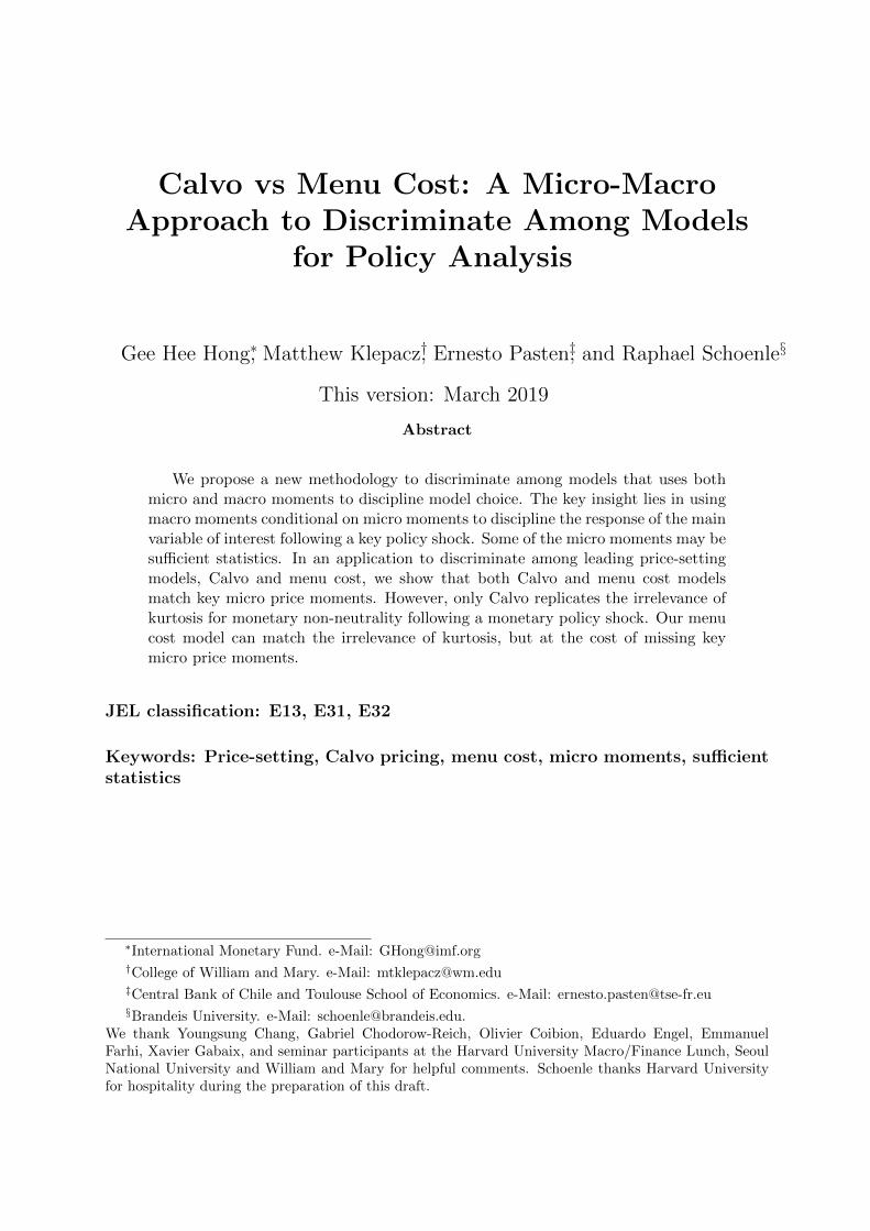
are shown in Figure 2. Consistent with the findings in Romer and Romer (2004), we find

that monetary policy shocks begin to yield price responses with at least 24 months lag.

We also observe the small “price puzzle” that is typically found using this measure.

First, consistent with our findings using FAVAR, we find that low price change

frequency industries have a smaller price response to the monetary shock than the high

frequency industries. This implies that they have a larger real output response. Only the

price series with high frequency shows a meaningful response to monetary shocks after 30

months, while the series with low frequency series does not. In the second panel we see

the impulse response when the industries are grouped by kurtosis of price changes. As we

found in the FAVAR analysis, there is no significant difference in cumulative response of

inflation to monetary policy shocks when observations are categorized based on kurtosis in

the middle panel. In response to the expansionary monetary policy shock, price responses

are observed after 35 quarters for the both high kurtosis price series and low kurtosis price

series. This is contrary to the reactions of inflation when observations are categorized

based on frequency and kurtosis over frequency. Similar results to the frequency grouping

can be observed when price series are split based on kurtosis over frequency in the final

21

3 6 9 12 15 18 21 24 27 30 33 36 39 42 45 48

Months

-0.5

-0.4

-0.3

-0.2

-0.1

0

0.1

0.2

0.3

0.4

0.5

0.6

0.7

0.8

0.9

1

Pe

rce

nt

Above Median

Below Median

a Frequency

3 6 9 12 15 18 21 24 27 30 33 36 39 42 45 48

Months

-0.5

-0.4

-0.3

-0.2

-0.1

0

0.1

0.2

0.3

0.4

0.5

0.6

0.7

0.8

0.9

1

Per

cent

Above MedianBelow Median

b Kurtosis

3 6 9 12 15 18 21 24 27 30 33 36 39 42 45 48

Months

-0.5

-0.4

-0.3

-0.2

-0.1

0

0.1

0.2

0.3

0.4

0.5

0.6

0.7

0.8

0.9

1

Per

cent


c Kurtosis/Frequency

Figure 2: Romer and Romer Monetary Policy Shock IRF

Note: In all three figures, “Above Median” and “Below Median” refer to the impulse response functionof industries whose pricing moment is above or below the median value of that statistic for all industries.Estimated impulse responses of sectoral prices to a one percent decrease in the RR policy series areshown.

panel.

IV Model

In this section we first demonstrate the inadequacy of micro pricing moments in

determining monetary non-neutrality in a one sector menu cost model. We then fully

specify a multi-sector pricing model that can match micro pricing facts as well as generate

sectoral impulse responses to monetary shocks.

A. One Sector Menu Cost Model

This section uses a standard, second-generation menu cost model to study how pricing

moments affect monetary non-neutrality. Firms can change prices by paying a menu cost

χ, or with some small probability α they can change the price for free. Idiosyncratic

productivity shocks arrive at rate pz with volatility σz and persistence ρz. The firm

productivity shock set up is the same as in Midrigan (2011).

The baseline model is calibrated to match price-setting statistics from the CPI micro

data during the period 1988-2012 documented by Vavra (2014).8. We then undertake a

comparative static exercise where we vary one pricing moment at a time to understand

8We define the fraction of small price changes as those less than 1% in absolute value and take thisdata from Luo and Villar (2015) This enables us to more directly compare small price changes acrossindustries in the multi-sector analysis.

22

High Low Low MediumParameter Baseline Frequency Frequency Kurtosis Kurtosis

χ 0.0071 0.0033 0.0087 0.0107 0.0087pz 0.053 0.086 0.0652 0.076 0.0652σz 0.16 0.173 0.147 0.126 0.147ρz 0.65 0.98 0.78 0.75 0.78α 0.03 0.03 0.03 0.03 0.03

Table 1: Model Parameters CPI Calibration

Note: The table shows the model parameters that are internally calibrated for each economy. χ denotesthe menu cost of adjusting prices, pz the probability that log firm productivity follows an AR(1) processwith standard deviation σz, ρz the persistence of idiosyncratic probability shocks, and α is the probabilityof a free price change.

High Low Low MediumMoment Data Baseline Frequency Frequency Kurtosis Kurtosis

Frequency 0.11 0.11 0.15 0.08 0.11 0.11Fraction Up 0.65 0.65 0.62 0.67 0.63 0.64Average Size 0.077 0.077 0.077 0.077 0.077 0.077Fraction Small 0.12 0.16 0.13 0.13 0.13 0.14Kurtosis 6.4 6.4 6.4 6.4 4.7 5.5KurtosisFrequency

58.2 57.6 42.6 81.8 42.2 50.1

Table 2: Frequency Comparative Static

Note: Monthly CPI data moments taken from Vavra (2014) and are calculated using data from 1988-2014.

the importance of each for monetary non-neutrality. The moments we examine are price

change frequency and kurtosis of price changes. This exercise also demonstrates if the

ratio of kurtosis over frequency is a sufficient statistic for monetary non-neutrality in a

simple menu cost model, or rather if it is a function of one of the underlying moments.

The five internally calibrated parameters that determine the price-setting moments

are in Table 1 and the associated price-setting statistics are in Table 2. The model does

a good job matching all the pricing moments from the data for the five calibrations we

examine.

The table shows that we are able to vary one pricing moment at a time, while

holding the others fixed. Monetary non-neutrality is measured by examining the impact

of a one time permanent expansionary monetary shock on real output. The monetary

shock increases nominal output by 0.002, a one month doubling of the nominal output

growth rate. The real effects of monetary shocks are then the cumulative consumption

23

1 2 3 4 5 6 7 8 9 10 11 120

0.1

0.2

0.3

0.4

0.5

0.6Consumption IRF

Kurtosis = 6.4, Frequency=.11Kurtosis = 6.4, Frequency=.15Kurtosis = 6.4, Frequency=.08Kurtosis = 4.7, Frequency=.11Kurtosis = 5.5, Frequency=.11

Figure 3: Consumption IRF Comparison

Note: Impulse response of output to a one time permanent increase in log nominal output of size 0.002for different calibrations.

impact due to the shock. From Figure 3, the results confirm that monetary non-neutrality

is a negative function of frequency in a menu cost model. The impulse response functions

also show that as kurtosis of price changes decreases, it causes monetary non-neutrality

to increase9.

The results also show that kurtosis over frequency does not make clear predictions

for monetary non-neutrality. According to the sufficient statistic approach of Alvarez

et al. (2016), the real output effect is completely determined by these two parameters.10

Yet the figure shows that varying frequency or kurtosis while holding the ratio constant

delivers different cumulative consumption responses. This can be seen by comparing the

high frequency and low kurtosis calibration. Increasing frequency and decreasing kurtosis

both decrease the ratio, but they cause the total consumption response to move in opposite

directions relative to the baseline calibration.

This stylized one sector model has shown that monetary non-neutrality does not

have a one to one relationship with kurtosis of price changes and that the kurtosis over

frequency ratio does not have a linear relationship with monetary non-neutrality. The

frequency of price changes exhibits a strong negative relationship with monetary non-

neutrality.

9We repeat this exercise using the model of Midrigan (2011) who more explicitly models firm multi-product pricing. We find the same relationship as in our model, that monetary non-neutrality falls askurtosis increases while holding frequency of regular price changes constant.

10A key assumption to deliver this sufficiency result is the normality of cost shocks. Our quantitativemodel features leptokurtic productivity shocks such as in Midrigan (2011).

24

B. Multi-Sector Pricing Model

This section now presents a multi-sector pricing model in order to demonstrate which

price-setting models can replicate the ordering of impulse response functions. The

quantitative pricing model nests both a second generation menu cost model as well as

the Calvo pricing model. The multi-sector model follows Nakamura and Steinsson (2010)

where there is some probability of a free Calvo price change and each sector has sector

specific pricing behavior. It also includes leptokurtic idiosyncratic productivity shocks as

in Midrigan (2011) as well as aggregate productivity shocks.

B.1 Households

A standard menu cost model of price-setting is now presented. The household side is

standard. Households maximize current expected utility, given by

Et

∞∑τ=0

βt[log(Ct+τ )− ωLt+τ

](18)

They consume a continuum of differentiated products indexed by i. The composite

consumption good Ct is the Dixit-Stiglitz aggregate of these differentiated goods,

Ct =

[ ∫ 1

0

ct(z)θ−1θ dz

] θθ−1

(19)

where θ is the elasticity of substitution between the differentiated goods.

Households decide each period how much to consume of each differentiated good.

For any given level of spending in time t, households choose the consumption bundle that

yields the highest level of the consumption index Ct. This implies that household demand

for differentiated good z is

ct(z) = Ct

(pt(z)

Pt

)−θ(20)

where pt(z) is the price of good z at time t and Pt is the price level in period t, calculated

as

Pt =

[ ∫ 1

0

pt(z)1−θdz

] 11−θ

(21)

25

A complete set of Arrow-Debreu securities is traded, which implies that the budget

constraint of the household is written as

PtCt + Et[Dt,t+1Bt+1] ≤ Bt +WtLt +

∫ 1

0

πt(z)dz (22)

where Bt+1 is a random variable that denotes state contingent payoffs of the portfolio of

financial assets purchased by the household in period t and sold in period t+1. Dt+1 is

the unique stochastic discount factor that prices the payoffs, Wt is the wage rate of the

economy at time t, πt(i) is the profit of firm i in period t. A no ponzi game condition is

assumed so that household financial wealth is always large enough so that future income

is high enough to avoid default.

The first order conditions of the household maximization problem are

Dt,t+1 = β(CtPt

Ct+1Pt+1

) (23)

Wt

Pt= ωCt (24)

where equation (23) describes the relationship between asset prices and consumption, and

(24) describes labor supply.

B.2 Firms

In the model there are a continuum of firms indexed by i and industry j. The production

function of firm i is given by

yt(i) = Atzt(i)Lt(i) (25)

where Lt(i) is labor rented from households. At are aggregate productivity shocks and

zt(i) are idiosyncratic productivity shocks.

Firm i maximizes the present discounted value of future profits

Et

∞∑τ=0

Dt,t+τπt+τ (i) (26)

where profits are given by:

26

πt(i) = pt(i)yt(i)−WtLt(i)− χj(i)WtIt(i) (27)

It(i) is an indicator function equal to one if the firm changes its price and equal to zero

otherwise. χj(i) is the sector specific menu cost. The final term indicates that firms must

hire an extra χj(i) units of labor if they decide to change prices with probability 1−αj, or

may change their price for free with probability αj.11 This is the “CalvoPlus” parameter

from Nakamura and Steinsson (2010) that enables the model to encapsulate both a menu

cost as well as a pure Calvo model. In the menu cost model this parameter is set such

that a small probability of receiving a free price change enables the model to generate

small price changes, while in the Calvo model set up it is calibrated to the frequency of

price changes with an infinite menu cost.

Total demand for good i is given by:

yt(i) = Yt

(pt(i)

Pt

)−θ(28)

The firm problem is to maximize profits in (27) subject to its production function (25),

demand for its final good product (28), and the behavior of aggregate variables.

Aggregate productivity follows an AR(1) process:

log(At) = ρAlog(At−1) + σAνt (29)

where νt ∼ N(0,1)

The log of firm productivity follows a mean reverting process with leptokurtic shocks:

logzt(i) =

ρzlogzt−1(i) + σz,jεt(i) with probability pz,j

logzt−1(i) with probability 1− pz,j,(30)

where εt(i) ∼ N(0,1).

Nominal aggregate spending follows a random walk with drift:

log(St) = µ+ log(St−1) + σsηt (31)

where St = PtCt and ηt ∼ N(0,1).

11This is a reduced form modeling device representing multiproduct firms like in Midrigan (2011).

27

The state space of the firms problem is an infinite dimensional object because the

evolution of the aggregate price level depends on the joint distribution of all firms’ prices,

productivity levels, and menu costs. It is assumed that firms only perceive the evolution

of the price level as a function of a small number of moments of the distribution as in

Krusell and Smith (1998). In particular, we assume that firms use a forecasting rule of

the form:

log(PtSt

) = γ0 + γ1logAt + γ2log(Pt−1St

) + γ3(log(Pt−1St

) ∗ logAt) (32)

The accuracy of the rule is checked using the maximum Den Haan (2010) statistic

in a dynamic forecast. The model is solved recursively by discretization and simulated

using the non-stochastic simulation method of Young (2010).

B.3 Calibration

For the model discrimination exercise we have a set of parameters common to all sectors.

The discount rate is set to β = (0.96)112 as the model is monthly. The elasticity of

substitution is set to θ = 4 as in Nakamura and Steinsson (2010).12 The nominal shock

process is calibrated to match the mean growth rate of nominal GDP minus the mean

growth rate of real GDP and the standard deviation of nominal GDP growth over the

period of 1998 to 2012. This implies µ = 0.002 and σs = 0.0037. Finally the model

is linear in labor so we calibrate the productivity parameters to match the quarterly

persistence and standard deviation of average labor productivity from 1976-2005. This

gives ρA = 0.8925 and σA = 0.0037.

The second set of parameters is calibrated internally to match micro pricing moments.

These are the menu cost χj, the probability of an idiosyncratic shock, pz,j, the volatility

of idiosyncratic shocks σj, and the probability of a free price change αj. For all models

evaluated we use two sectors to match our baseline empirical results.

12While other papers in the literature set the elasticity of substitution to higher numbers such as 7 inGolosov and Lucas (2007), this lowers the average mark up, but the ordered price level response to amonetary shock would not change.

28

V Results

This section now presents our main model results. We first show that a multi-sector

menu cost model that matches micro pricing moments is unable to match the ordering of

impulse response functions for all slices of the data. In particular, it predicts differences in

response when sectors are split by kurtosis, contradicting the empirical results. However,

we show a multi-sector Calvo model consistent with micro pricing data is able to match

all impulse response function orderings. Lastly, we do a comparative static exercise where

we vary sectoral parameters to show that a menu cost model can match the irrelevance of

kurtosis for impulse response functions. However, this comes at the cost of missing micro

price moments.

We calibrate the two sector model to match three different cuts of the data: frequency,

kurtosis, and kurtosis over frequency. For each of the parameterizations we calculate

the price-setting moments for each industry, then calibrate each sector to the average

price-setting moments above or below the median statistic of interest. Price-setting

moments for all calibrations are in Table 3. In the menu cost calibration we are matching

frequency of price changes, average size of price changes, fraction of small price changes,

and kurtosis of price changes for each sector. These four moments pin down four

sector specific parameters. The parameters are the menu cost χj, the probability of an

idiosyncratic productivity shock pz,j, volatility of idiosyncratic productivity shocks σz,j,

and the probability of a free price change αj. The parameter values are shown in Table

4. In the Calvo variation of the model, price changes are fully time dependent, so we set

the menu cost to infinity and no longer target the fraction of small price changes. This

leaves three parameters to target frequency, average size, and kurtosis of price changes.

The average price-setting moments across sectors show large differences in the

moment of interest, yet surprisingly minor differences in other moments. In the frequency

data cut, the low frequency of price changes is 0.14 while the high frequency of price

changes is 0.35. Yet, the kurtosis of price changes is 6.2 and 6.7 respectively, which enables

the model to demonstrate how a change in frequency impacts monetary non-neutrality.

The kurtosis data cut also exhibits a similar pattern when the average kurtosis across the

low and high sectors varies by 4.0 to 9.0, while frequency is only differs by one percent

per month. The kurtosis over frequency split exhibits large differences in both frequency

and kurtosis, where the two pricing moments work together to generate the low and high

29

Frequency CalibrationLow Frequency High Frequency

Sector SectorMoment Data MC Calvo Data MC Calvo

Frequency 0.14 0.14 0.14 0.35 0.35 0.34Average Size 0.073 0.074 0.071 0.062 0.061 0.060Fraction Small 0.46 0.32 0.35 0.31 0.42 0.49Kurtosis 6.2 6.1 6.4 6.7 6.7 6.9KurtosisFrequency

44.8 42.8 46.2 19.3 18.8 20.1

Kurtosis CalibrationLow Kurtosis High Kurtosis



17.0 16.9 17.6 36.0 32.3 37.5

Kurtosis/Frequency CalibrationLow Kurtosis/Frequency High Kurtosis/Frequency



15.7 16.3 16.3 45.0 40.0 47.2

Table 3: Multi-sector Pricing Moments

Note: Monthly pricing moments calculated using PPI data from 1998-2005. For all calibrations, eachpricing moment is calculated at the 6 digit NAICS level. The average pricing moment is then calculatedfor industries above and below the median statistic of interest. Fraction small is the fraction of pricechanges less than one percent in absolute value. The MC column denotes the menu cost model calibrationand the Calvo column denotes the Calvo model calibration.

30

Frequency CalibrationLow Frequency High Frequency

Sector SectorParameter MC Calvo MC Calvo

χj 0.052 ∞ 0.00047 ∞pz,j 0.073 0.139 0.16 0.244σz,j 0.167 0.15 0.141 0.136αj 0.11 0.139 0.22 0.348



χj 0.109 ∞ 0.001 ∞pz,j 0.254 0.56 0.10 0.12σz,j 0.10 0.11 0.21 0.185αj 0.212 0.236 0.138 0.25

Kurtosis/Frequency CalibrationLow Kurtosis/Frequency High Kurtosis/Frequency


χj 0.0021 ∞ 0.012 ∞pz,j 0.183 0.425 0.08 0.104σz,j 0.115 0.108 0.205 0.188αj 0.175 0.301 0.17 0.183

Table 4: Multi-sector Model Calibration

Note: The table shows the model parameters that are internally calibrated for each economy where thesector is indexed by j. χj denotes the menu cost of adjusting prices, pz,j the probability that log firmproductivity follows an AR(1) process with standard deviation σz,j , and αj is the probability of a freeprice change. The MC column denotes the menu cost model calibration and the Calvo column denotesthe Calvo model calibration.

31

response respectively.

In our model discrimination exercise, we ask if each model is capable of replicating

the ordering of the empirical impulse response to a monetary shock. In each model

we simulate the effects of an expansionary monetary shock. Log nominal output has a

permanent increase of 0.002 and we trace out the effects to the price level.13 The results

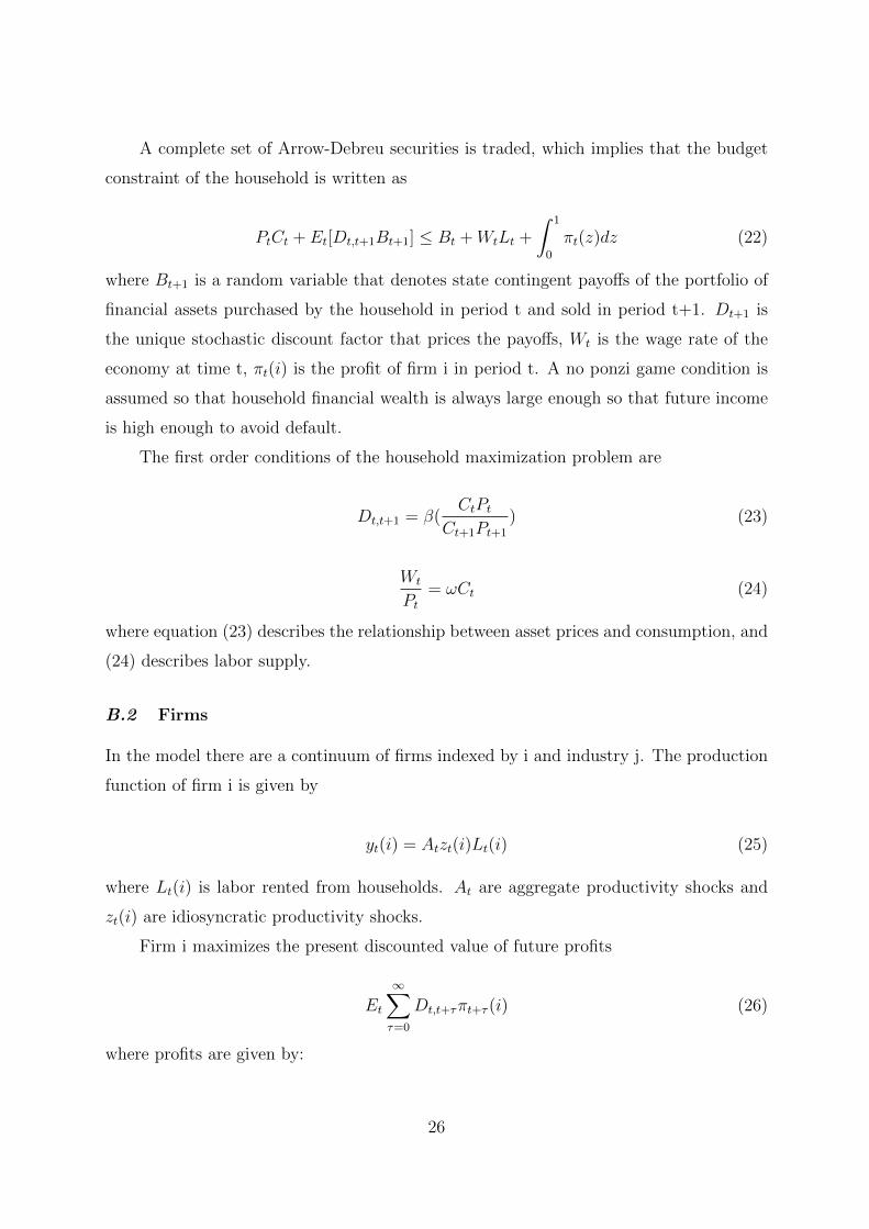
are in Figure 4. In the top left panel, we show the price response relative to trend in the

menu cost model when the data are cut by frequency of price changes. As expected, the

high frequency of price changes sector incorporates more of the monetary shock to prices

on impact and more quickly fully integrates the shock into the price level. These results

are consistent with the FAVAR and narrative evidence.

The price level impulse responses from the menu cost model where we slice the data

by kurtosis of price changes are in the top center panel. The panel shows a substantial

difference in impulse response functions. The high kurtosis sector has a larger price

response to a monetary shock and therefore a smaller consumption response. This

model, while consistent with the micro pricing moments, is inconsistent with the empirical

impulse response evidence. In both the FAVAR and narrative evidence, when the data is

ordered by kurtosis there is no difference in the average response. This evidence suggests

that kurtosis of price changes is not informative for monetary non-neutrality.14

The top right panel shows the impulse response when the data are cut by kurtosis

over frequency. Consistent with Alvarez et al. (2016), the sector with high kurtosis over

frequency has a smaller price response and therefore has a larger consumption response

to a monetary shock.

We now show that a Calvo model is able to match the ordering of impulse responses

in all three cuts of the data. The bottom left panel in Figure 4 shows that a high frequency

sector has a larger price response. The middle panel shows that the Calvo model can also

match the irrelevance of kurtosis. The distance between the impulse response functions

is small relative to all other orderings. Lastly, the bottom right panel shows the Calvo

13We choose the size of the shock to match a one month doubling of the nominal output growth rate.In the menu cost model the size of the nominal shock will affect the fraction of price adjusters and thushave implications for the impulse response function, while in the Calvo model the size of the shock doesnot impact non-neutrality.

14While kurtosis does not have effects on the ordering of the price response to a monetary shock, itcan be informative for discriminating among models. Any model that gives a prediction for monetarynon-neutrality should be consistent with kurtosis of price changes not affecting the price response to amonetary shock.

32

1 2 3 4 5 6 7 8 9 10 11 120.2

0.4

0.6

0.8

1

1.2

1.4

1.6

1.810-3


a Frequency Menu Cost

1 2 3 4 5 6 7 8 9 10 11 120.4

0.6

0.8

1

1.2

1.4

1.6

1.810-3


b Kurtosis Menu Cost

1 2 3 4 5 6 7 8 9 10 11 120.4

0.6

0.8

1

1.2

1.4

1.6

1.810-3


c Kurtosis/Frequency Menu Cost

1 2 3 4 5 6 7 8 9 10 11 120

0.2

0.4

0.6

0.8

1

1.2

1.4

1.610-3


d Frequency Calvo

1 2 3 4 5 6 7 8 9 10 11 120.2

0.4

0.6

0.8

1

1.2

1.4

1.610-3


e Kurtosis Calvo

1 2 3 4 5 6 7 8 9 10 11 120

0.2

0.4

0.6

0.8

1

1.2

1.4

1.610-3


f Kurtosis/Frequency Calvo

Figure 4: Multi-sector Model Monetary Policy Shock IRF

Note: In all six figures, “Above Median” and “Below Median” refer to the impulse response functionof the sector calibrated to match the pricing moments above or below the median value of the statisticfor all industries. The top row shows the menu cost model results and the bottom row shows the Calvomodel results. Model calibration noted under each figure. Impulse responses of sectoral prices in responseto a permanent increase in money.

model when the sectors are split by kurtosis over frequency. The model replicates the

larger price response of the low kurtosis over frequency sector, and therefore the smaller

consumption response.

These models have different implications for monetary non-neutrality. Consistent

with prior evidence, all three Calvo model calibrations have greater monetary non-

neutrality, as measured by the cumulative output response to a monetary shock, compared

to all three menu cost model calibrations. In both the Calvo and menu cost models, the

frequency calibration has greater monetary non-neutrality than the other two calibrations.

This suggests that sectors with the lowest frequency have outsize influence on monetary

non-neutrality in the aggregate, consistent with the argument made in Nakamura and

Steinsson (2010).

While the menu cost model does not match irrelevance of kurtosis in the impulse

responses, it is possible to parameterize it to do so. But this comes at the cost of missing

33

the micro price moments. We show this using a comparative static exercise. We start

this exercise from the baseline multi-sector menu cost parameterization based on the

kurtosis of price changes. Then we take one sectoral parameter at a time in the set

Θ ∈ (χj, σz,j, pz,j, αj), and vary it while holding all other parameters constant. The

parameter is indexed by industry j, allowing us to vary one sector parameter while holding

the other constant. The search of parameters is done within the values of the two baseline

parameters.

The empirical impulse response function for kurtosis of price changes does not differ.

We search for the set of parameters that minimizes the sum of squared deviation in

the price level impulse response to a monetary shock between the two sectors, low and

high kurtosis. The search shows that the two parameters that decrease the distance

between the responses the most are the volatility of idiosyncratic shocks and the menu

cost. However the menu cost parameter allows us to decrease distance between responses

the most, when the low kurtosis sector has a high menu cost consistent with the baseline

specification and the high kurtosis sector needs to increase the menu cost relative to the

baseline specification, while all other parameter values are set to their original value. The

impulse response associated with the minimum distance occurs when χ1 = 0.109 and

χ2 = 0.008, and all other parameters are fixed at their baseline calibration. The impulse

response functions are shown in Figure 5. The figure shows that it is possible to have

no difference in impulse response when we have heterogeneous sectors. Yet this comes at

the cost of missing the micro pricing moments for the high kurtosis sector. In particular,

both the frequency of price changes as well as kurtosis need to be decreased for the second

sector to match the two impulses. The associated moments are shown in Table 5.

This section shows that our new methodology can discriminate among different

pricing models. A menu cost model is not able to fit all micro moments as well as match

the sectoral price response to a monetary shock when calibrated to match above and

below-median kurtosis sectors. Yet, a Calvo model is able to match the impulse response

ordering in all three calibrations of the model. While this is not evidence that the Calvo

model is the correct micro-foundation for price stickiness, it shows that when studying

the effects of monetary shocks on pricing behavior it fits the empirically implied response

better. Our exercise further demonstrates that the menu cost model needs an additional

feature to fit the key variable response of interest to monetary shocks and therefore be

34

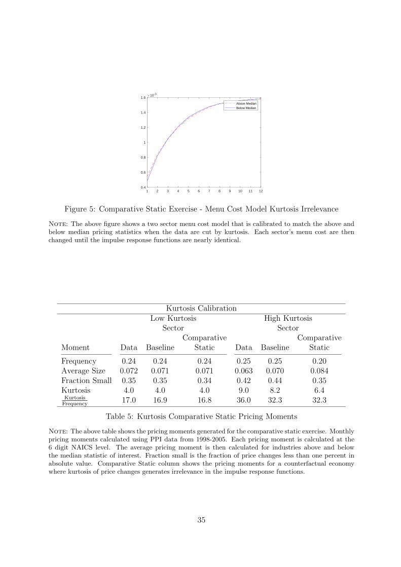
1 2 3 4 5 6 7 8 9 10 11 120.4

0.6

0.8

1

1.2

1.4

1.610-3


Figure 5: Comparative Static Exercise - Menu Cost Model Kurtosis Irrelevance

Note: The above figure shows a two sector menu cost model that is calibrated to match the above andbelow median pricing statistics when the data are cut by kurtosis. Each sector’s menu cost are thenchanged until the impulse response functions are nearly identical.


Sector SectorComparative Comparative

Moment Data Baseline Static Data Baseline Static


17.0 16.9 16.8 36.0 32.3 32.3

Table 5: Kurtosis Comparative Static Pricing Moments

Note: The above table shows the pricing moments generated for the comparative static exercise. Monthlypricing moments calculated using PPI data from 1998-2005. Each pricing moment is calculated at the6 digit NAICS level. The average pricing moment is then calculated for industries above and belowthe median statistic of interest. Fraction small is the fraction of price changes less than one percent inabsolute value. Comparative Static column shows the pricing moments for a counterfactual economywhere kurtosis of price changes generates irrelevance in the impulse response functions.

35

useful for policy analysis.

VI Conclusion

We have proposed a new methodology to discriminate among models that uses both

micro and macro moments to discipline model choice. The key insight of our method

lies in tying the use of macro moments to discipline the response of the main variable of

interest following a key policy shock to the simultaneous choice of micro moments that

pin down model behavior. Some of these micro moments may be sufficient statistics.

To demonstrate the power of our method, we apply it to discriminate among leading

pricing models that are widely used in policy making, Calvo and menu cost. First, we

show empirically that a lower frequency of price changes is related to larger consumption

responses to monetary policy shocks. Kurtosis is not an empirically sufficient statistic for

the real effects of monetary shocks, but as a derivative, kurtosis over frequency is. Both

Calvo and menu cost models match key micro price moments and the impulse response

ordering if we consider frequency and kurtosis over frequency as moments. However,

only Calvo replicates the irrelevance of kurtosis. In a menu cost model, kurtosis is not

a sufficient statistic for monetary non-neutrality by itself, and kurtosis over frequency is

not sufficient unless it has a one-to-one relationship with frequency. Our menu cost model

can match the irrelevance of kurtosis, but at the cost of missing key micro price moments.

Future work might consider quantitative refinements of the second step of our

methodology for our application. Currently, the second step consists of a non-parametric

comparison of impulse response orderings in models and the data. An extension in our

application would also match the particular shapes of impulse response functions. Such

an exercise would require adding a number of features to the model to replicate inertial

and hump-shaped behavior of aggregate inflation and quantities, as stressed by Christiano

et al. (2005).

36

References

Alvarez, F., M. Beraja, M. Gonzalez-Rozada, and P. A. Neumeyer (2019). Fromhyperinflation to stable prices: Argentina’s evidence on menu cost models. TheQuarterly Journal of Economics 134 (1), 451–505.

Alvarez, F., H. Le Bihan, and F. Lippi (2016, October). The real effects of monetaryshocks in sticky price models: A sufficient statistic approach. American EconomicReview 106 (10), 2817–51.

Bachmann, R., R. Caballero, and E. M. R. A. Engel (2013). Aggregate implicationsof lumpy investment: New evidence and a dsge model. American Economic Journal:Macroeconomics 5 (4), 29–67.

Berger, D., R. Caballero, and E. Engel (2018). Missing Aggregate Dynamics andVAR Approximations of Lumpy Adjustment Models. Working papers, NorthwesternUniversity, Department of Economics.

Bernanke, B. S., J. Boivin, and P. Eliasz (2005). Measuring the effects of monetary policy:A factor-augmented vector autoregressive (favar) approach. The Quarterly Journal ofEconomics 120 (1), 387–422.

Bils, M., P. J. Klenow, and O. Kryvtsov (2003). Sticky Prices and Monetary PolicyShocks. Federal Reserve Bank of Minneapolis Quarterly Review (27), 2–9.

Boivin, J., M. P. Giannoni, and I. Mihov (2009, March). Sticky prices and monetary policy:Evidence from disaggregated us data. American Economic Review 99 (1), 350–84.

Christiano, L. J., M. Eichenbaum, and C. L. Evans (2005). Nominal rigidities and thedynamic effects of a shock to monetary policy. Journal of Political Economy 113 (1),1–45.

Cravino, J., T. Lan, and A. A. Levchenko (2018, June). Price stickiness along theincome distribution and the effects of monetary policy. CEPR Discussion Papers 12967,C.E.P.R. Discussion Papers.

Dotsey, M. and A. L. Wolman (2018, July). Inflation and Real Activity with Firm LevelProductivity Shocks. Working Papers 18-19, Federal Reserve Bank of Philadelphia.

Eichenbaum, M. (2018a). Modern dsge models: Theory and evidence. Presentation,https://youtu.be/Wgboaq9 Kx4 min. 9.46’ - 10.58’, Nobel Symposium, Swedish Houseof Finance.

Eichenbaum, M. (2018b). Modern dsge models: Theory and evidence. Discussion,https://youtu.be/69rLdiWRoUs min. 23.39’ -24.31’, Nobel Symposium, Swedish Houseof Finance.

Gagnon, E. (2009). Price setting during low and high inflation: Evidence from mexico.The Quarterly Journal of Economics 124 (3), 1221–1263.

Golosov, M. and R. Lucas (2007). Menu costs and phillips curves. Journal of PoliticalEconomy 115 (2), 171–199.

Gorodnichenko, Y. and M. Weber (2016). Are sticky prices costly? Evidence from thestock market. American Economic Review 106 (1), 165–199.

Gourieroux, C., A. Monfort, and E. Renault (1993). Indirect inference. Journal of AppliedEconometrics , 85–118.

37

Haan, W. J. D. (2010). Assessing the accuracy of the aggregate law of motion in modelswith heterogeneous agents. Journal of Economic Dynamics and Control 34 (1), 79 –99. Computational Suite of Models with Heterogeneous Agents: Incomplete Marketsand Aggregate Uncertainty.

Karadi, P. and A. Reiff (2018). Menu costs, aggregate fluctuations, and large shocks.Technical report, Forthcoming, AEJ: Macroeconomics.

Khan, A. and J. K. Thomas (2008). Idiosyncratic shocks and the role of nonconvexitiesin plant and aggregate investment dynamics. Econometrica 76 (2), 395–436.

Kim, S. (2016). Quality, price stickiness, and monetary policy. Working paper, BrandeisUniversity.

Klenow, P. J. and B. A. Malin (2011). Chapter 6 - Microeconomic Evidence on Price-Setting. Volume 3 of Handbook of Monetary Economics, pp. 231 – 284. Elsevier.

Luo, S. and D. Villar (2015). The skewness of the price change distribution: A newtouchstone for sticky price models. FEDS Working Paper 2017-028, Board of Governorsof the Federal Reserve System, Finance and Economics Discussion Series.

Mackowiak, B., E. Moench, and M. Wiederholt (2009). Sectoral price data and modelsof price setting. Journal of Monetary Economics (56), 78–99.

McFadden, D. (1989). A method of simulated moments for estimation of discrete responsemodels without numerical integration. Econometrica 57 (5), 995–1026.

Midrigan, V. (2011). Menu costs, multiproduct firms, and aggregate fluctuations.Econometrica 79 (4), 1139–1180.

Nakamura, E. and J. Steinsson (2010). Monetary non-neutrality in a multi-sector menucost model. Quarterly Journal of Economics 125 (3), 961–1013.

Nakamura, E. and J. Steinsson (2018). Identification in macroeconomics. The Journal ofEconomic Perspectives 32 (3), 59–86.

Nakamura, E., J. Steinsson, P. Sun, and D. Villar (2018). The elusive costs ofinflation: Price dispersion during the u.s. great inflation. The Quarterly Journal ofEconomics 133 (4), 1933–1980.

Romer, C. D. and D. H. Romer (2004). A new measure of monetary shocks: Derivationand implications. American Economic Review 94 (4), 1055–1084.

Romer, D. H. and C. D. Romer (2000, June). Federal reserve information and the behaviorof interest rates. American Economic Review 90 (3), 429–457.

Smith, J. A. (1993). Estimating Nonlinear Time-series Models Using Simulated VectorAutoregressions, Volume 8.

Vavra, J. (2014). Inflation dynamics and time-varying volatility: New evidence and an Ssinterpretation. The Quarterly Journal of Economics 129 (1), 215–258.

Young, E. R. (2010). Solving the incomplete markets model with aggregate uncertaintyusing the krusell-smith algorithm and non-stochastic simulations. Journal of EconomicDynamics and Control 34 (1), 36 – 41.

38

.05

.1.1

5.2

Fre

quen

cy

0 5 10 15Kurtosis

a Low Frequency Sectors

.2.4

.6.8

Fre

quen

cy

0 5 10 15 20Kurtosis

b High Frequency Sectors

12

34

56

Kur

tosi

s

0 .2 .4 .6 .8Frequency

c Low Kurtosis Sectors

510

1520

Kur

tosi

s

.1 .2 .3 .4 .5 .6Frequency

d High Kurtosis Sectors

Figure 6: Comparative Static Exercise

Note: The figures above plot average industry price setting statistics by group. Panels a and b in thetop row plot kurtosis against frequency for the sectors with above-median and below-median frequency.Panels c and d in the bottom row plot frequency against kurtosis for the sectors with above-median andbelow-median kurtosis.

A Appendix

A. Sectoral Characteristics

We plot the 154 industry level price setting moments in figure 6 when the industries are

separated into above- and below-median values of a moment of interest. These results

show the heterogeneity in price setting moment across industries to compare to the average

values in table 3.

Table 3 shows the average kurtosis values are 6.2 and 6.7 for the low and high

frequency sectors respectively. The top row of figure 6 shows there is not a strong

39

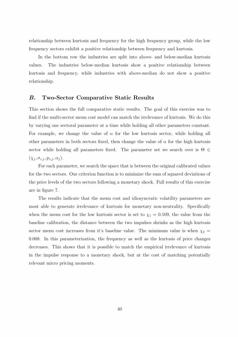
relationship between kurtosis and frequency for the high frequency group, while the low

frequency sectors exhibit a positive relationship between frequency and kurtosis.

In the bottom row the industries are split into above- and below-median kurtosis

values. The industries below-median kurtosis show a positive relationship between

kurtosis and frequency, while industries with above-median do not show a positive

relationship.

B. Two-Sector Comparative Static Results

This section shows the full comparative static results. The goal of this exercise was to

find if the multi-sector menu cost model can match the irrelevance of kurtosis. We do this

by varying one sectoral parameter at a time while holding all other parameters constant.

For example, we change the value of α for the low kurtosis sector, while holding all

other parameters in both sectors fixed, then change the value of α for the high kurtosis

sector while holding all parameters fixed. The parameter set we search over is Θ ∈(χj, σz,j, pz,j, αj).

For each parameter, we search the space that is between the original calibrated values

for the two sectors. Our criterion function is to minimize the sum of squared deviations of

the price levels of the two sectors following a monetary shock. Full results of this exercise

are in figure 7.

The results indicate that the menu cost and idiosyncratic volatility parameters are

most able to generate irrelevance of kurtosis for monetary non-neutrality. Specifically

when the menu cost for the low kurtosis sector is set to χ1 = 0.109, the value from the

baseline calibration, the distance between the two impulses shrinks as the high kurtosis

sector menu cost increases from it’s baseline value. The minimum value is when χ2 =

0.008. In this parameterization, the frequency as well as the kurtosis of price changes

decreases. This shows that it is possible to match the empirical irrelevance of kurtosis

in the impulse response to a monetary shock, but at the cost of matching potentially

relevant micro pricing moments.

40

0.14 0.15 0.16 0.17 0.18 0.19 0.2 0.21

2

0

0.1

0.2

0.3

0.4

0.5

0.6

0.7

0.8

0.9

1

Cum

ulat

ive

Dis

tanc

e

10-6

1=0.138

1=0.16

1=0.19

1=0.212

a Calvo Plus Probability - α

0.1 0.15 0.2 0.25

Pz,2

0

0.1

0.2

0.3

0.4

0.5

0.6

0.7

0.8

0.9

1

Cum

ulat

ive

Dis

tanc

e

10-6

Pz,1

=0.1

Pz,1

=0.15

Pz,1

=0.2

Pz,1

=0.254

b Probability of Shock - Pz

0.1 0.11 0.12 0.13 0.14 0.15 0.16 0.17 0.18 0.19 0.2

z,2

0

0.1

0.2

0.3

0.4

0.5

0.6

0.7

0.8

0.9

1

Cum

ulat

ive

Dis

tanc

e

10-6

z,1=0.1

z,1=0.135

z,1=0.17

z,1=0.21

c Idiosyncratic Volatility - σz

0.01 0.02 0.03 0.04 0.05 0.06 0.07 0.08 0.09 0.1

2

0

0.1

0.2

0.3

0.4

0.5

0.6

0.7

0.8

0.9

1

Cum

ulat

ive

Dis

tanc

e

10-6

1=0.001

1=0.02

1=0.05

1=0.109

d Menu Cost - χ

Figure 7: Comparative Static Exercise

Note: Cumulative distance between price impulse responses shown as each parameter value varies.Cumulative distance between impulse responses is defined as

∑T=12t=1 (Pt,1 − Pt,2)

2, where t is indexing

months after a positive monetary shock. The x-axis denotes the parameter value for the high kurtosissector, while each line indicates a different value of the parameter for the low kurtosis sector. Each panelvaries one parameter at a time.

41

calvo vs menu cost: a micro-macro approach to discriminate

Documents